What does perturbative QCD really have to say about neutron stars

Abstract

The implications of perturbative QCD (PQCD) calculations on neutron stars are carefully examined. While PQCD calculations above baryon chemical potential $\mu_{B}\sim 2.4$ GeV demonstrate the potential of ruling out a wide range of neutron star equations of state (EOSs), these types of constraints only affect the most massive neutron stars in the vicinity of the Tolman-Oppenheimer-Volkoff (TOV) limit, resulting in bounds on neutron star EOSs that are orthogonal to those from current or future astrophysical observations, even if observations near the TOV limit are made. Assuming the most constraining scenario, PQCD considerations favor low values of the speed of sound squared $C_{s}$ at high $\mu_{B}$ relevant for heavy neutron stars, but leave predictions for the radii and tidal deformabilities almost unchanged for all the masses. Such considerations become irrelevant if the maximum of speed of sound squared inside neutron stars does not exceed about $C_{s,\mathrm{max}}\sim 0.5$, or if the matching to PQCD is performed above $\mu_{B}\simeq 2.9$ GeV. Furthermore, the large uncertainties associated with the current PQCD predictions make it impossible to place any meaningful bounds on neutron star EOSs as of now. Interestingly, if PQCD predictions for pressure at around $\mu_{B}\simeq 2.4$ GeV is refined and found to be low ($\lesssim 1.5$ GeV/fm³), evidence for a soft neutron star inner core EOS would point to the presence of a strongly interacting phase dominated by non-perturbative physics beyond neutron star densities.

I Introduction

An ab initio QCD-based calculation of dense matter beyond a few times the nuclear saturation density ($n_{0}=0.16$ fm^-3) relevant for the interior of neutron stars remains challenging. This strongly interacting regime not only precludes perturbative calculations but also discourages applications of lattice methods due to the sign problem [1, 2, 3]. Such obstacles have deprived us of a clear understanding of neutron stars even though almost a century has passed since their conception by Landau and by Zwicky and Baade [4].

In contrast to the stagnation in this strongly coupled region, significant progress has been made at the low- and ultra high-density frontiers. On one hand, for baryon number densities below about $\sim 2n_{0}$, an effective description based on symmetries of QCD has proven fruitful in predicting the properties of neutron-rich matter. Dubbed chiral effective field theory ($\chi$EFT) [5, 6, 7], it allows for and arranges all possible operators respecting chiral symmetry through a power counting scheme [8, 9]. The result is a systematic expansion in nucleon momenta that not only enables calculations of the equations of state but also provides error estimates through order-by-order comparisons. For example, the recent next-to-next-to-next leading order (N3LO) calculation reveals that the $1\sigma$ uncertainties associated with the pressure of pure neutron matter (PNM) to be $\sim 10\%$ at $n_{B}=n_{0}$, and worsen to about $40\%$ at $2n_{0}$  [10]. On the other hand, at densities above $\sim 50-100n_{0}$, asymptotic freedom of QCD suggests perturbative treatments become valid and useful. The pioneering work of [11, 12] confirmed that cold quark matter resembles closely to a Fermi gas in this region, and has promoted significant efforts in simplifying and improving calculations for cold and dense QCD [13, 14, 15, 16, 17]. Given the scarcity of available information directly related to the phase of matter at supranuclear densities in between, gleaning as many insights as possible from both ends is a desirable undertaking.

That high-density PQCD calculations may place limits on NS EOSs through thermodynamic consistency requirements is well-known, and there is only a potential for constraints because the current uncertainties associated with PQCD predictions are simply too large to place meaningful bounds. However, a renewed wave of interest in this topic is recently generated by [18]. That letter, along with the subsequent papers including attempts to clarify it [19], are marred by several issues and have led to apparently widespread misunderstandings in the literature.

In this first paper of the series exploring the interplay between high- and low-density theoretical inputs we focus on the potential implications of PQCD calculations on neutron star EOSs. One objective is to clarify the misunderstandings on this subject. Specifically, it will be shown that due to our limited understanding of the QCD phase diagram only one type of the bounds derived from thermodynamic relations may be viewed as a constraint on NS EOSs. Furthermore, while pQCD  constraints do demonstrate the potential of ruling out a considerable region of EOSs, neutron star observables are barely affected by these high-density inputs, as bounds expected from PQCD are orthogonal to those based on astrophysics.

The rest of the paper is organized as follows. A simple parameterization of $\chi$EFT  EOSs is discussed in section II, and the PQCD EOS for cold quark matter is reviewed in section III. In section IV we review the thermodynamic relations at zero temperature that give rise to the conditions low- and high-density EOSs must satisfy. In section V we apply these bounds and carefully examine the underlying assumptions, the applicable ranges, and the consequence of such considerations. We conclude and outline future directions in section VI. Throughout the discussion we adopt the natural unit system in which $G=\hbar=c=1$.

II neutron star EOS

In this section we give an overview of the parameterization of neutron star EOSs used in this work. Details will be reported in  [20].

II.1 parameterizing $\chi$EFT  with correlated uncertainties

Recently, refs [21, 10] studied truncation errors of $\chi$EFT  based on the assumptions that its predictions for energy per particle admit a polynomial expansion in momenta, and that the unknown coefficients associated with higher order terms are natural in size. Using a Gaussian Process (GP) interpolant the authors inferred the size and characteristic length scales of the inter-density correlations of the polynomial coefficients, and used these to obtain extrapolated truncation errors. The resulting correlated uncertainties are encoded in the covariance matrix $\mathrm{Cov}(E_{i},E_{j})$ where $E_{i,j}$ are energies per particle at the ith and jth tabulated density points, excluding the rest mass. Although one can reconstruct the GP interpolant reported there and use it to generate EOS samples, this approach cannot be easily extended to construct beta-equilibrium EOSs that respect the underlying inter-density correlations.

Here, we present a minimal, faithful parameterization of the $\chi$EFT  calculations that captures not only the central values of the EOS but also the correlated truncation errors. The type of correlation we focus on is the inter-density correlation, as it is the most significant one for neutron-rich matter. At the core of this parameterization lies the eigenvalue decomposition (singular value decomposition) of the covariance matrix

$$USU^{T}=||\mathrm{Cov}(E_{i},E_{j})||.$$ (1)

The eigenvectors in $U$ are orthonormal since the covariance is symmetric. In particular, each eigenvector $U_{i}$ represents a correlation among different densities of the truncation error, with the $1\sigma$ variance given by the square root of its corresponding eigenvalue $\sqrt{\text{diag}(S)_{i}}$. For both the chiral potentials with $450$ MeV and $500$ MeV cutoffs reported in [10], the largest (second largest) entry in $\sqrt{\text{diag}(S)}$ accounts for about $\sim 90\%$ ($8\%$) of the variances encoded in the full covariance matrix, suggesting their corresponding eigenvectors, which shall be referred to as the most significant eigenvectors, are adequate for current and future astrophysical applications. This is true for calculations of both pure neutron matter (PNM) and symmetric nuclear matter (SNM), and for concreteness we will focus on the PNM EOS $E(n_{n})$ where $n_{n}$ is the neutron number density.

The two most significant eigenvectors form a set of orthogonal basis to describe the correlated uncertainties. Denote $E_{0}(n_{n})$ the central values of energy per particle predicted by $\chi$EFT, the proposed parameterization that incorporates correlated uncertainties takes the form

$$E(n_{n})=E_{0}(n_{n})+\sum_{i=1}^{2}a_{i}E_{i}(n_{n})+m_{n},\\ \quad\text{with }E_{i}(n_{n})=\sqrt{\text{diag}(S)_{i}}\ U_{i}(n_{n}).$$ (2)

Above, $m_{n}$ is the mass of neutrons, and the variance associated with each eigenvector is absorbed into the definition of basis functions $E_{i}(n_{n})$, so that the (uncorrelated) coefficients $a_{i}$ are independent identical draws from the standard normal distribution $\mathcal{N}(0,1)$. This procedure effectively projects out the high-dimensional covariance matrix to a lower dimension subspace spanned by the basis functions $E_{i=1,2}(n_{n})$ (not to be confused with $E_{i,j}$ in eq. 1).

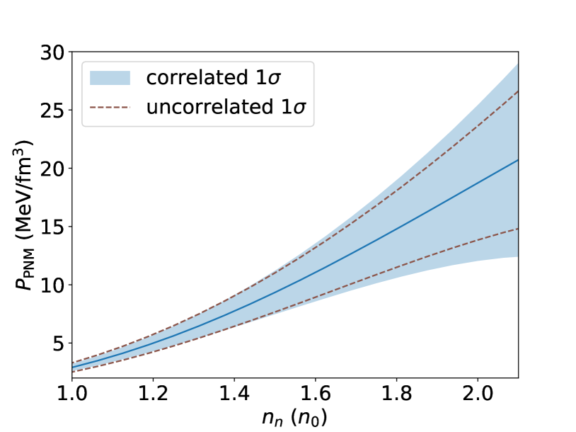
Figure 1: $\chi$EFT  predictions for the pressure of PNM and the associated uncertainties at N3LO. This EOS is based on the chiral potential with a $500$ MeV cutoff reported in [10]. The correlated truncation errors are obtained according to eq. 1 and eq. 2, and are shown as the blue band. The uncorrelated uncertainty (dashed) underestimates the error in pressure by as much as $30\%$ near $n_{B}=2n_{0}$, even though they agree on energy per particle within $10\%$ (not shown).

These basis functions, along with the central values for the EOS $E_{0}(n_{n})$, are well-behaved and can be faithfully fitted with polynomials. For optimal fittings, polynomials of degree $\gtrsim 4$ are sufficient as the fitted EOS as well as derivatives are stationary with increasing polynomial degrees. This allows us to turn the discrete tabulated EOS from $\chi$EFT  calculations to a compact, faithful, and continuous representation eq. 2. The resulting EOSs in this parameterization are shown in fig. 1. The pressure is calculated straightforwardly as $P=n_{n}^{2}(\mathrm{d}E/\mathrm{d}n_{n})$, and the $1\sigma$ upper and lower bounds of correlated errors are obtained by setting $a_{1}=a_{2}=\pm 1$ in eq. 2. For comparison, the uncorrelated $1\sigma$ errors obtained by taking the square root of $\text{diag}(||\mathrm{Cov}(E_{i},E_{j})||)$ are shown as dashed lines. The importance of inter-density correlations is evident as the dashed curve underestimates the error in pressure by almost $1/3$ near $n_{B}=2n_{0}$. In most cases inter-density correlations are positive is expected since the energy at a given point is less likely to be small if its neighboring points all predict large values.

We note that the EOS in eq. 2 can be parameterized either against number densities $n_{n}$ or Fermi momenta $k_{F}$. The covariance matrix obtained in [10] in fact involves $E(k_{F})$ tabulated on an equally spaced grid in Fermi momenta $k_{F}$, as inter-density correlations appear more natural on this grid. It is not straightforward to translate this GP interpolated EOS on the uniform grid of $k_{F}$ to another GP representation on a grid of different thermodynamic variables, as the physical inter-density correlations are not preserved in the process. This is a limitation due to GP where the kernels are transnational invariant. Here, choosing either $k_{F}$ or $n_{n}$ is fine since the correlations captured by the basis functions are invariant under change of variables. Interpolation by polynomials does introduce systematics, though a simple estimate by dropping half the points and reproducing them using the remaining data points seems to indicate they are controlled and no more than $\sim 5\%$.

This prescription works well for both pure neutron matter (PNM) and symmetric nuclear matter (SNM) EOSs, but we only take the PNM EOS from [22, 10]. The main consideration is that PNM is perturbative and its EOS may be convergent even if chiral EFT is shown to be non-renormalizable. The EOS for nuclear matter in beta-equilibrium is then constructed based on a series expansion in proton fraction $x_{p}=n_{p}/n_{B}$ described in  [23]. This approach incorporates nuclear saturation properties by imposing a boundary condition at $x_{p}=1/2$. Unlike those based on the parabolic expansion centered around $x_{p}=1/2$, the resulting beta-equilibrium EOS is only moderately sensitive to the properties of SNM. While we acknowledge that theoretical and experimental probes of SNM near and below saturation densities are very valuable inputs, they may suffer from currently unknown systematic uncertainties, as the recent neutron skin measurements might have indicated [24, 25]. Adding that neutron stars are mostly neutrons, we believe this informed and flexible approach is a noteworthy alternative to those in the literature for connecting nuclear physics to neutron star observables. For the purpose of this paper, the results are insensitive to the choices between SNM-centered or PNM-centered expansions, and we will only present results based on the latter. A systematic comparison of the two and careful examinations of low-energy nuclear inputs will be reported in another work focusing on low-density EOSs.

II.2 inner core EOS

For densities above $n_{\text{$\chi$EFT}}\simeq 1-2n_{0}$ where EFT is expected to break down, we adopt a family of parameterized sound of sound EOS that the author developed in [26]. It has not been published, though a few subsets have been reported elsewhere [27, 28, 29]. The details of this family of parameterizations will be reported in a separate work [20]. To the authors knowledge, this family of EOS is the most agnostic approach with minimal assumptions. We have checked that the results below are robust against different choices of priors on EOS parameters (implicit or explicit), and across different subsets of inner core parameterizations.

III perturbative QCD

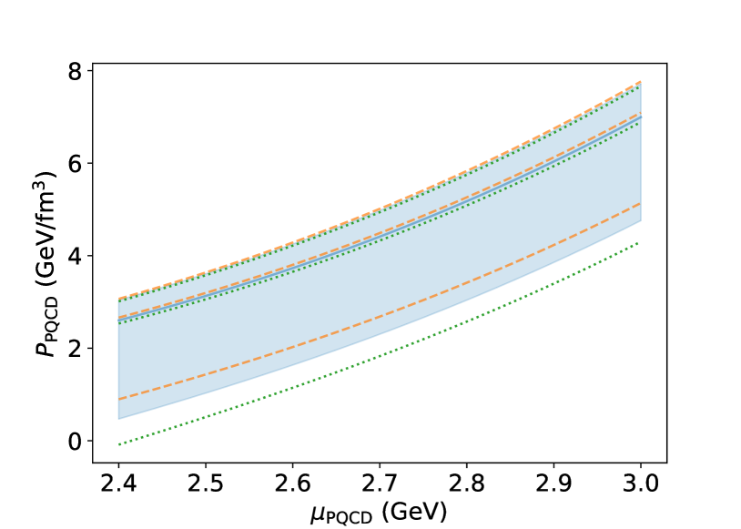
Figure 2: The PQCD EOS up to N2LO. The blue band shows the renormalization scale uncertainties assuming $\alpha_{s}(2~{}\text{GeV})=0.2994$, where the lower boundary corresponds to $X=1$, the upper boundary corresponds to $X=4$, and the blue solid line in between to $X=2$. The green (orange) lines mark the same ranges for $X=[1,2,4]$, but assume the $0.5\sigma$ upper (lower) bound of $\alpha_{s}(2~{}\text{GeV})$ (see appendix A).

At asymptotically large chemical potentials, QCD becomes perturbative and renders useful an expansion in the strong coupling $\alpha_{s}$. The calculation of cold quark matter EOS up to N2LO is first performed in [11, 12] in the momentum space subtraction renormalization scheme, and remains the state-of-art full order calculation. Subsequent works have formulated it in the more popular $\overline{\mathrm{MS}}$ scheme[30, 14], in which the pressure of unpaired quark matter with $N_{f}=3$ massless flavors is given by

$$P=N_{f}\frac{(\mu_{B}/3)^{4}}{12\pi^{2}}\left\{1-\frac{2}{\pi}\alpha_{s}-\frac{N_{f}}{\pi^{2}}\alpha_{s}^{2}\log{\alpha_{s}}\right.-\frac{\alpha_{s}^{2}}{\pi^{2}}\\ \times\left.\left[{c_{1}+N_{f}\left(\log\frac{N_{f}}{\pi}-c_{2}\right)}+\left(11-\frac{2}{3}N_{f}\right)\log{X}\right]\right\}.$$ (3)

Above, $c_{1}=18-11\log{2}$, $c_{2}=0.535832\ldots$ are numerical constants. The renormalization scale $\bar{\Lambda}$ is implicit in $\alpha_{s}\equiv\alpha_{s}(\bar{\Lambda})$ and is conveniently parameterized in terms of the baryon chemical potential as $X=\bar{\Lambda}/(\mu_{B}/3)$. Since the quark chemical potential $\mu_{q}=\mu_{B}/3$ is the characteristic scale of the problem, one can expect a good choice of renormalization scale to be close to it ($X\sim 1$). In [31] the authors compared predictions of eq. 3 to an exactly solvable large $N_{f}$ limit where they varied $X$ between $1/2$ and $2$, and found that the large $N_{f}$ prediction lies somewhere in $X\in[1,2]$, and is a bit closer to $X=2$. Based on this observation, as well as empirical evidence from hot PQCD calculations, the dense quark matter community appears to have adopted $X=1,2,4$ as fiducial values to provide estimates for renormalization scale uncertainties [14]. This range is shown in fig. 2 as the blue band.

We note that the appearance of $X$ in eq. 3 is an artifact of the perturbation theory since physical observables shall be independent of it. Once higher order corrections are included, PQCD predictions are expected to show diminished sensitivity towards the renormalization scale, assuming PQCD is converging at given $\mu_{B}$. In this sense, the uncertainty associated with $X$ is in fact a truncation error of the perturbation series. Efforts estimating the truncation error based on naturalness considerations are underway and will be reported in future work.

Another (often neglected) source of errors comes from the running of $\alpha_{s}$. In the main text we use a two-loop solution of $\alpha_{s}$ that is consistent with eq. 3. The uncertainty associated with the inferred value of $\alpha_{s}$ can have a sizable impact on PQCD predictions. This is depicted in fig. 2 as the dashed and dotted lines. The effect is especially prominent towards lower values of $X$, where a percentage difference in the reference value $\alpha_{s}(2~{}\text{GeV})$ would shift the pressure on the order of $\simeq 20-50\%$. Note that we do not claim the choice adopted here is the best option. A few other options are discussed in appendix A. We merely point out that the uncertainties associated with $\alpha_{s}$ have to be properly accounted for before claiming constraints, and that extracting $\alpha_{s}$ in the infrared is inherently challenging. For a recent review see [32].

Recently, partial N3LO results are reported in [15, 33, 17] for the soft gluon sector by resumming diagrams using EFT techniques [34, 35, 36]. The newly obtained contribution is the first positive term in the series, and hence predicts higher pressure at given chemical potentials. However, if calculations of cold dense QED [37] or hot QCD [38, 39] were to be of any guide, the unknown hard and mixed contributions at N3LO are likely negative, and the net contribution at full order N3LO may drive the pressure even lower than that of eq. 3. In light of this, we take the cautious approach and use the N2LO PQCD EOS in the main text, commenting on the impacts of the partial N3LO corrections and presenting the results in appendix B.

IV zero-temperature thermodynamic consistency requirements

The consistency conditions implicit in thermodynamic relations at zero temperature are most easily seen in the $\mu_{B}-P$ plane, where the pressure $P$ as a function of the baryon chemical potential $\mu_{B}$ is continuous and differentiable. Furthermore, $P(\mu_{B})$ is a convex function since

$$\mathrm{d}P/\mathrm{d}\mu_{B} =n_{B},$$ (4)

$$\frac{\mathrm{d}\log n_{B}}{\mathrm{d}\log\mu_{B}} =C_{s}^{-1},\quad 0\leq C_{s}\leq 1.$$ (5)

where $C_{s}$ is the speed of sound squared, a non-negative quantity for stable phases. Causality also imposes the additional requirement that $C_{s}\leq 1$. Together these relations suggest that for a given separation in chemical potential $\Delta\mu_{B}=\mu_{H}-\mu_{L}$ between two arbitrary points which we label “L” and “H”, there exists an upper and a lower bound on $\Delta P=P_{H}-P_{L}$, where $P_{H}=P(\mu_{H})$ and $P_{L}=P(\mu_{L})$.

To obtain the upper bound on $\Delta P$, we would like to have the highest possible values for the derivative $\frac{\mathrm{d}P}{\mathrm{d}\mu_{B}}=n_{B}$ throughout the range $[\mu_{L},\mu_{H}]$. The schematics for $n_{B}$ is shown in fig. 3. At $\mu_{L}$, in order to get the largest value of the number density, we introduce a first order phase transition which raises $n_{B}$ by an arbitrary amount at the expense of zero increase in $\mu_{B}$. But since the slope in the $\log n_{B}-\log\mu_{B}$ plane is the inverse of the speed of sound squared, which must be no less than 1 as demanded by causality, jumps in the number density that are too large would make it impossible to reach $n_{H}$ at $\mu_{H}$. To find the maximum of this value of $n_{L}$ we start from $(\mu_{H},n_{H})$ and follows the line with the least possible slope $C_{s}^{-1}=1$ down to $\mu_{L}$, where it gives

$$n_{L}^{\mathrm{max}}=n_{H}\exp\left[\int^{\log\mu_{L}}_{\log\mu_{H}}\mathrm{d}\log\mu_{B}\right]=n_{H}\frac{\mu_{L}}{\mu_{H}}.$$ (6)

This point is labeled in red in fig. 3. From there, the EOS we just followed from $n_{H}$ downwards is the only allowed path to reach $(\mu_{H},n_{H})$ without violating causality $C_{s}\leq 1$. In fact, this EOS predicts the largest possible number densities between $\mu_{L}$ and $\mu_{H}$. Therefore this construction, as shown in red in fig. 3, leads to the largest possible $\Delta P$ given by

$$\Delta P_{\mathrm{max}}=\frac{n_{H}}{\mu_{H}}\int^{\mu_{H}}_{\mu_{L}}\mathrm{d}\mu_{B}\mu_{B}=\frac{n_{H}\mu_{H}}{2}\left[1-\left(\frac{\mu_{L}}{\mu_{H}}\right)^{2}\right].$$

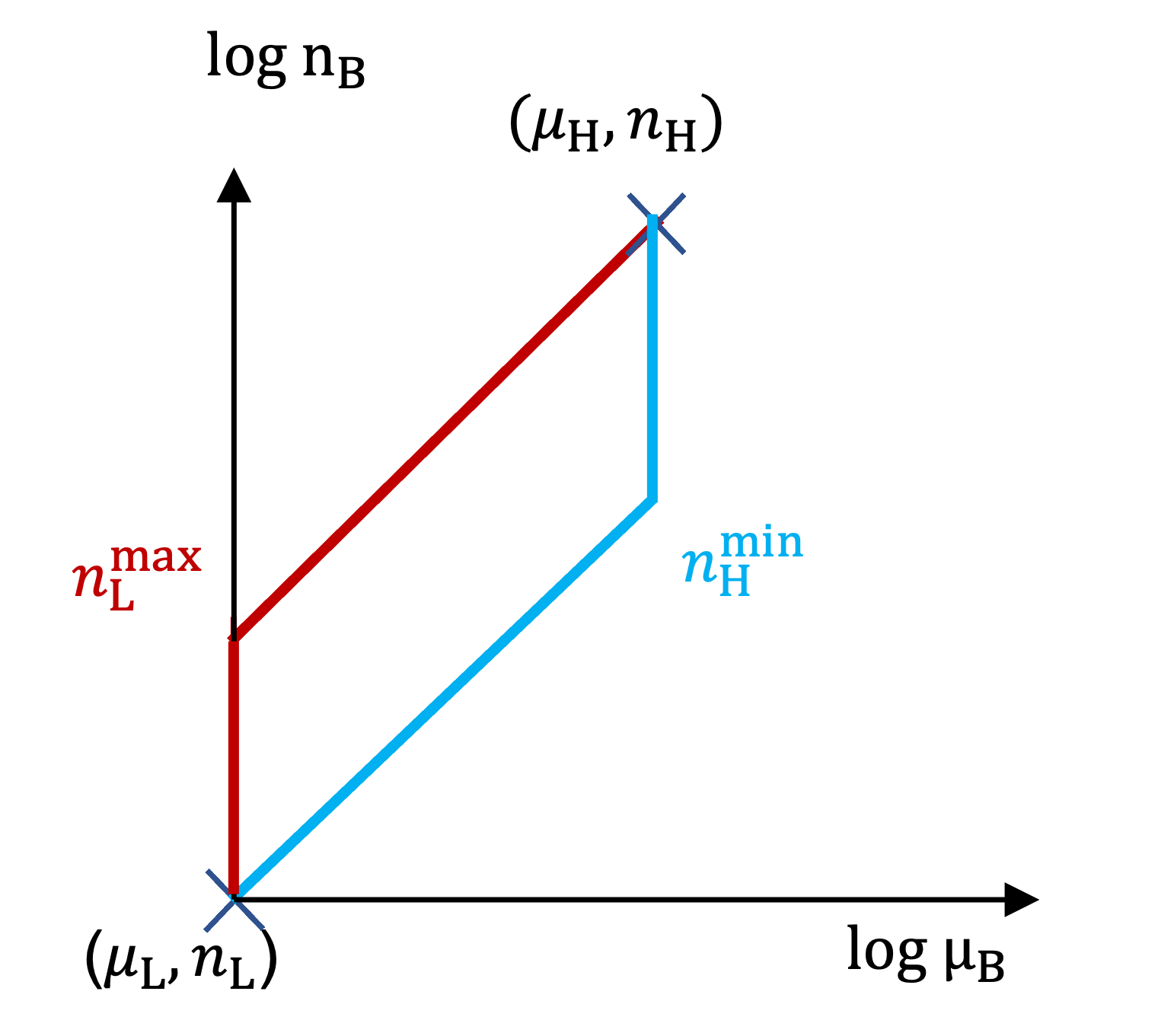
Figure 3: The maximally stiff (blue) and soft (red) EOSs between $\mu_{L}$ and $\mu_{H}$ that yield $\Delta P_{\mathrm{min}}$ and $\Delta P_{\mathrm{max}}$ respectively.

Following similar arguments one finds that the EOS depicted in blue in fig. 3 bears the lowest number densities between $\mu_{L}$ and $\mu_{H}$. It starts at $\mu_{L}$ with a constant $C_{s}=1$ and reaches $\mu_{H}$ with a number density

$$n_{H}^{\mathrm{min}}=n_{L}\exp\left[\int_{\log\mu_{L}}^{\log\mu_{H}}\mathrm{d}\log\mu_{B}\right]=n_{L}\frac{\mu_{H}}{\mu_{L}},$$ (7)

then climbs to $n_{H}$ via a first order phase transition. The resulting lower bound on $\Delta P$ reads

$$\Delta P_{\mathrm{min}}=\frac{n_{L}}{\mu_{L}}\int^{\mu_{H}}_{\mu_{L}}\mathrm{d}\mu_{B}\mu_{B}=\frac{n_{L}\mu_{L}}{2}\left[\left(\frac{\mu_{H}}{\mu_{L}}\right)^{2}-1\right].$$

It is not a coincidence that the constructions shown in red and blue that yielded $\Delta P_{\mathrm{max}}$ and $\Delta P_{\mathrm{min}}$ are the maximally soft and maximally stiff EOSs first posited in [40]. For low-density EOSs that are soft, i.e., predict large values of $P_{L}$, one needs stiff EOSs in the region between $\mu_{L}$ and $\mu_{H}$ to reach the given high-density point $(\mu_{H},n_{H},p_{H})$. And if the low-density EOS is too soft such that $\Delta P=P_{H}-P_{L}<\Delta P_{\mathrm{min}}$, even the maximally stiff EOS between $\mu_{L}$ and $\mu_{H}$ would overshoot $p_{H}$ at $\mu_{H}$; In the other extreme, if the low-density EOS is too stiff predicting pressures that are too low, even the maximally soft EOS in the region $[\mu_{L},\mu_{H}]$, which gives rise to $\Delta P_{\mathrm{max}}$, is unable to bring the pressure to $P_{H}$ at $\mu_{H}$.

Below, we will take the PQCD predictions at $\mu_{\text{pQCD}}\equiv\mu_{H}\sim 2.5-3$ GeV as a boundary condition and study the implications of $\Delta P_{\mathrm{max}}$ and $\Delta P_{\mathrm{min}}$

$$\Delta P_{\mathrm{max}} =\frac{n_{\text{pQCD}}\mu_{\text{pQCD}}}{2}\left[1-\left(\frac{\mu_{L}}{\mu_{\text{pQCD}}}\right)^{2}\right],$$ (8)

$$\Delta P_{\mathrm{min}} =\frac{n_{L}\mu_{L}}{2}\left[\left(\frac{\mu_{\text{pQCD}}}{\mu_{L}}\right)^{2}-1\right],$$ (9)

on neutron star EOSs. While in principle both eq. 8 and eq. 9 can incorporate PQCD calculations around $\sim 50n_{0}$ to put constraints on NS EOSs at lower densities, we shall demonstrate that only eq. 8 may be considered as a constraint, given our current understanding of the zero temperature QCD phase diagram.

V Implications for neutron stars

Since the central densities of stars at the TOV limit are the maximum attainable values (which we shall refer to as the TOV points for NS EOSs) for stable neutron stars relevant to astrophysics, we will take the low-density matching point $\mu_{L}$ in eqs. 8 and 9 to be at or below the TOV point for each NS EOS throughout the discussion.

Below, only the existence of two-solar-mass NSs [41, 42, 43, 44] is explicitly taken into account by the ensembles of the EOSs considered in the main text. We shall demonstrate that PQCD constraints do not affect NS global observables such as the radius $R$ and the tidal deformability $\Lambda$, and will explicitly show this in appendix C by taking into account additional astrophysical inputs on $R$ and $\Lambda$.

V.1 the $\Delta P_{\mathrm{min}}$ bound, or not?

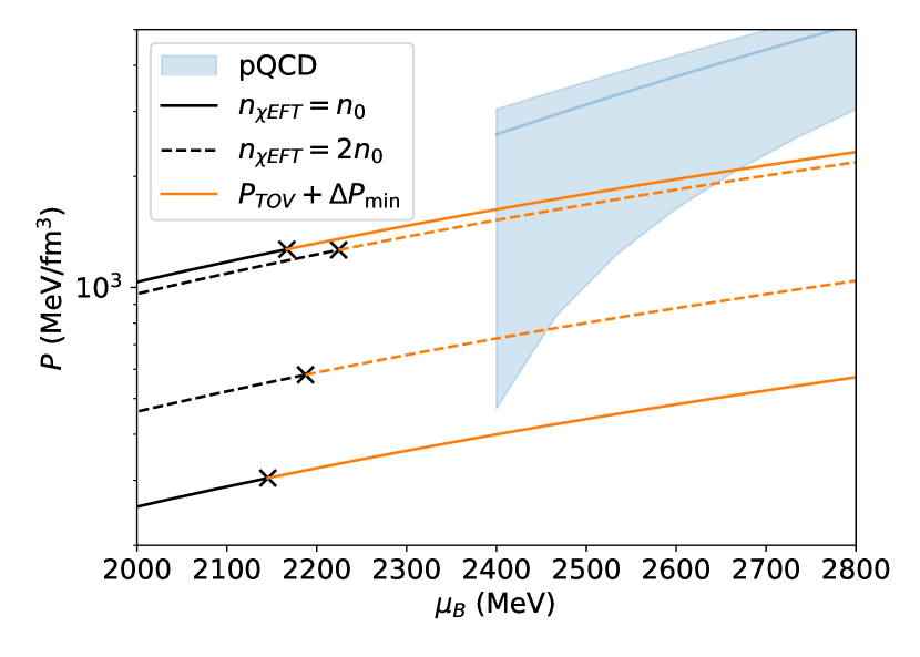
Figure 4: The $\Delta P_{\mathrm{min}}$ bound eq. 9 applied to the maximally stiff and soft EOSs. The blue band shows the range of PQCD predictions and is the same as in fig. 2. The solid (dashed) black lines show NS EOSs based on $\chi$EFT  up to $n_{\text{$\chi$EFT}}=1.0n_{0}$ ($2.0n_{0}$) then switched to the maximally stiff and soft inner core EOSs. They are terminated at their respective TOV points, marked by black crosses. From there the $\Delta P_{\mathrm{min}}$ bound is applied to each EOS and is shown in orange. For the four limiting cases shown, while eq. 10 is always satisfied for PQCD EOSs with $X\gtrsim 1.5$, it is violated by those that predict very low pressure ($X\simeq 1$) below $\mu_{\text{pQCD}}\lesssim 2.6$ GeV. However, this shall not be viewed as a constraint on NS EOSs, see main text.

We first discuss the implications of $\Delta P_{\mathrm{min}}$. For a given low-density matching point $\mu_{L}$, $n_{L}$, and $P_{L}$, eq. 9 is a sole function of $\mu_{\text{pQCD}}$, and it puts a lower limit on $P_{\text{pQCD}}\equiv P(\mu_{\text{pQCD}})$, requiring

$$P(\mu_{\text{pQCD}})\geq P_{L}+\Delta P_{\mathrm{min}}(\mu_{\text{pQCD}}).$$ (10)

Violation of eq. 10 might occur if $P_{L}$ is too high, so that $P_{L}+\Delta P_{\mathrm{min}}$ overshoots $P_{\text{pQCD}}$ at the high-density matching point. This bound is strongest when matched at $\mu_{L}=\mu_{t}ov$ and is shown in Figure 4. For the NS EOSs that follow $\chi$EFT  up to $n_{\text{$\chi$EFT}}=n_{0},2n_{0}$ then switched to the maximally soft inner core EOS, $P_{\text{pQCD}}$ lie well above the bound $P_{\text{TOV}}+\Delta P_{\mathrm{min}}(\mu_{\text{pQCD}})$ for both $X=2,4$, but that predicted by $X=1$ does not. Hence these soft NS EOSs are in tension with PQCD predictions for $X\lesssim 1.4$.

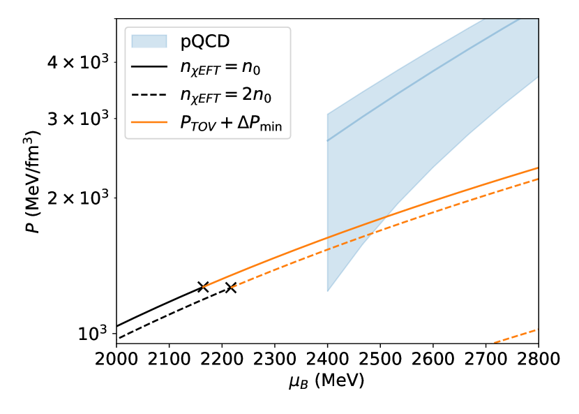
Figure 10: Similar to fig. 4 except that the partial N3LO contribution is included. The effect of eq. 9 becomes weaker. As explained earlier this is not a constraint on NS EOSs. Since predictions for $P_{\text{pQCD}}$ at given $X$ are not expected to be invariant when higher order terms are included in PQCD, and the uncertainties in $n_{\text{pQCD}}$ are relatively controlled, it is more convenient to directly parameterize PQCD uncertainties in terms of $P_{\text{pQCD}}$. For instance, if $P_{\text{pQCD}}(2.4\text{GeV})=1.2$ GeV/fm³ and the maximally soft EOSs are confirmed by astrophysics, assuming the ground state is a CFL phase the pairing gap needs to be at least $\sim 50~{}\text{MeV}$.

The obvious caveat is that the current uncertainties of PQCD are considerably wild, especially near lower values of $X$ relevant for this constraint. Violations of this kind only occur for PQCD EOSs with $X\gtrsim 1.4$, or equivalently $P_{\text{pQCD}}(2.4\text{GeV})\lesssim 1.5$ GeV/fm³. The partial N3LO contribution raises $P_{\text{pQCD}}$ and renders this constraint weaker, see fig. 10 in appendix B.

The critical flaw in the above argument lies in the assumption that the unpaired quark matter described by pQCD  is known to be the true ground state around $\mu_{\text{pQCD}}\simeq 2.4~{}\text{GeV}$. Below $\bar{\Lambda}\sim\mu_{q}\simeq\text{GeV}$ the strong coupling constant $g_{s}=\sqrt{4\pi\alpha_{s}}$ that appears in the Lagrangian is above 1, suggesting non-perturbative effects could still dominate in this regime. Since the determination of ground state requires knowledge of all possible phases, including the unpaired quark matter and other exotic strongly-interacting phases QCD might admit, we are unable to make the call based on the PQCD EOS alone, even if its uncertainty can be significantly reduced. On the other hand, the laws of thermodynamics favor the phase with the lowest grand potential (highest pressure) at given chemical potentials. For instance, assuming the ground state at $\mu_{B}=2.4$ GeV is a color-flavor-locked (CFL) color superconductor  [45, 46, 47] with a gap around $\Delta\sim 100$ MeV ($\Delta\sim 50$ MeV if the partial N3LO contribution is included, see fig. 10.) , the tension shown in Fig 2 goes away. Indeed, if future astrophysical observations support rather soft inner core NS EOSs, and higher order corrections narrow down $P_{\text{pQCD}}(2.4~{}\text{GeV})$ to be below $\sim 1.5~{}\text{GeV}/\text{fm}^{3}$, violation of this $\Delta P_{\mathrm{min}}$ bound could be evidence of non-perturbative phenomena in the zero temperature QCD phase diagram around $\mu_{B}\simeq 2.4-3~{}\text{GeV}$.

V.2 the $\Delta P_{\mathrm{max}}$ bound

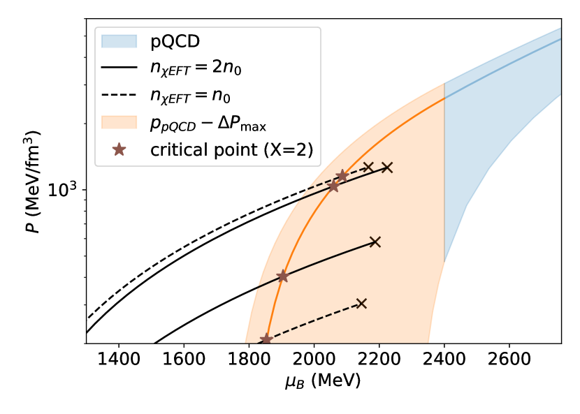
Figure 5: The $\Delta P_{\mathrm{max}}$ bound eq. 11 applied to the maximally stiff and soft NS EOSs when matched to PQCD at $2.4$ GeV. The blue band shows the range of PQCD predictions up to N2LO, and is the same as in fig. 2. The solid (dashed) black lines depict EOSs based on $\chi$EFT  up to $n_{\text{$\chi$EFT}}=1.0n_{0}$ ($2.0n_{0}$) then switched to the maximally stiff and soft EOSs. They are truncated at their respective TOV points, marked by black crosses. The bound eq. 11 is shown in orange. For the four extreme EOSs shown, while eq. 11 is always satisfied for PQCD EOSs with $X\lesssim 1.3$, a large portion of the PQCD parameter space at $\mu_{\text{pQCD}}=2.4$ GeV demonstrates the potential of constraining these NS EOSs. The brown stars labeled “critical” mark the lowest densities at which the bound is violated. Although they can be quite far from the TOV points, suggesting large pieces of NS EOSs are ruled out, these segments are only relevant for stars very close to the TOV limit.

For a given PQCD EOS and high-density matching point $\mu_{\text{pQCD}}$, eq. 8 is a sole function of $\mu_{L}$. Again since NSs do not probe beyond densities at the center of the TOV limit, we take $\mu_{L}$ to be at or below the TOV point of each NS EOS. This leads to a lower bound on the pressure of the NS EOS

$$P(\mu_{L})\geq P_{\text{pQCD}}-\Delta P_{\mathrm{max}}(\mu_{L}).$$ (11)

To understand the implications of eq. 11, we begin by looking at the limiting cases, the maximally stiff and soft NS EOSs. They are shown in fig. 5, and are both in tension with PQCD predictions when matched at $\mu_{\text{pQCD}}=2.4$ GeV for renormalization scales $X\gtrsim 1.6$. The maximally soft EOSs predict the highest possible pressure at given $\mu_{B}$, and yet these pressures at around $2.2$ GeV are still too low to allow for a construction consistent with thermodynamics that connects it to the majority of the PQCD EOSs at $2.4$ GeV. On the other end of the spectrum, the pressure of the maximally stiff EOSs is the lowest possible at given $\mu_{B}$. Owning to the huge uncertainties associated with the PQCD EOS, even these extremely low pressures cannot be ruled out as they are still compatible with eq. 11 assuming $X\lesssim 1.2$.

It immediately follows that a wide range of NS EOSs are at risk of being constrained by eq. 11, since the maximally stiff and soft EOSs are expected to bracket all possibilities and are themselves subject to this bound, and that for those that might be in tension with PQCD EOSs, they cannot be ruled out as of yet. Figure 6 shows predictions for the radius of $2M_{\odot}$ NSs and the tidal deformability of $1.4M_{\odot}$ stars for about a million randomly generated samples following $\chi$EFT  up to $n_{0}$. Because $\mu_{\text{TOV}}$ is the maximum of $\mu_{B}$ for an NS EOS, checking eq. 11 at the TOV point alone is sufficient to determine if an NS EOS is compatible with given PQCD predictions or not. Upon imposing eq. 11 at $\mu_{\text{pQCD}}=2.4$ GeV assuming $X=4$, the most optimistic scenarios for PQCD constraints, about $20\%$ of the samples in this pool are excluded . This constraint, however, does not affect appreciably the ranges of $R_{2.0\mathrm{M_{\odot}}}$ and $\Lambda_{1.4\mathrm{M_{\odot}}}$, or correlations between the two. While there is a minor preference for slightly higher $R_{2.0\mathrm{M_{\odot}}}$ in the posterior distributions, as the excluded samples tend to cluster around the lower ends of $R_{2.0\mathrm{M_{\odot}}}$ (because $2M_{\odot}$ is further away from $M_{\text{TOV}}$ for stiffer EOSs, see below), this shift is no more than $0.2$ km. Consequently, any possible constraints on NS EOSs from eq. 11 will be almost orthogonal to those from current or proposed astrophysical observations.

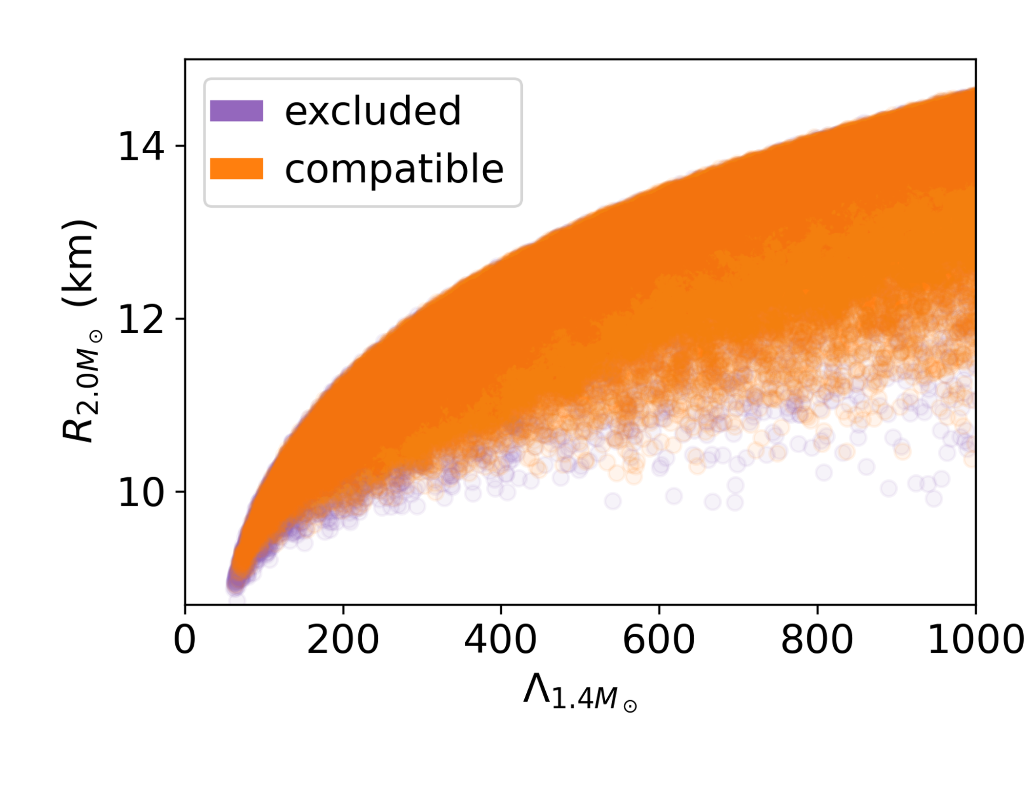
Figure 6: NS observables for EOSs that are compatible with (orange) and excluded by (purple) eq. 11 when matched to PQCD at $\mu_{\text{pQCD}}=2.4$ GeV assuming $X=4$. The posterior is not appreciably different from the prior, suggesting the PQCD constraint is mostly orthogonal to that from current or future astrophysical observations. The underlying samples are generated according to the parameterizations described in section II and follow $\chi$EFT  up to $n_{0}$. $\Lambda_{1.4\mathrm{M_{\odot}}}$ is truncated at 1000 as values greater than this are strongly disfavored by GW170817 [49, 50], although in this ensemble $\Lambda_{1.4\mathrm{M_{\odot}}}$ can reach about 3000. PQCD constraints do not affect those stiff cases either.

That PQCD constraints do not have appreciable influences on neutron star observables can be understood by noting that only stars very close to the TOV limit are affected. This latter point might seem counter-intuitive, given that considerable portions of NS EOSs shown in fig. 5 appear to violate eq. 11. For instance, taking $X=2$ (the central solid line), the violation of eq. 11 starts at $\mu_{B}\simeq 1.8$ GeV for the maximally stiff EOSs, whereas the TOV points of these EOSs are located at $\mu_{B}\simeq 2.2$ GeV. For convenience, we shall refer to the densities where NS EOSs cross the line $P=P_{\text{pQCD}}-\Delta P_{\mathrm{max}}$ as the “critical” point. The critical points are marked as brown stars in fig. 5. For the maximally stiff EOS that follows the upper $3\sigma$ $\chi$EFT  up to $n_{0}$ ($2n_{0}$), the mass of the star it predicts with $\mu_{\mathrm{crit}}$ as the central chemical potential is $M_{\mathrm{crit}}\equiv M(\mu_{\mathrm{crit}})=3.99~{}\mathrm{M_{\odot}}$ ($2.92~{}\mathrm{M_{\odot}}$), a value only differs from the TOV limit $M_{\text{TOV}}=4.04~{}\mathrm{M_{\odot}}$ ($2.89~{}\mathrm{M_{\odot}}$) by about one percent. The radius of the star at the critical point $R_{\mathrm{crit}}\equiv R(M_{\mathrm{crit}})$ is also not too different from $R_{\text{TOV}}$. For the maximally soft EOS with $n_{\text{$\chi$EFT}}=n_{0}$ ($2n_{0}$), $R_{\mathrm{crit}}$ is about $0.1$ km ($0.1$ km) larger than $R_{\text{TOV}}=8.6$ km ($8.9$ km), and for the maximally stiff EOS follows $\chi$EFT  up to $n_{0}$ ($2n_{0}$), $R_{\mathrm{crit}}$ is about $0.4$ km ($0.3$ km) larger than $R_{\text{TOV}}=17.4$ km ($12.9$ km) . This is a ubiquitous feature shared by all the solutions to the TOV equations. Indeed, for all the EOS samples considered, the derivative of NS masses with respect to central baryon chemical potentials for two-solar-mass stars are small $\left(\mathrm{d}M/\mathrm{d}\mu_{c}\right)_{2\mathrm{M_{\odot}}}\lesssim 10^{-2}~{}\mathrm{M_{\odot}}/\text{MeV}$ and decreases rapidly for heavier stars.

The analysis above hints at possible ways of modifying an EOS that is in tension with given PQCD calculations so that it satisfies eq. 11. Since the segment below $\mu_{\mathrm{crit}}$ of such an EOS already complies with eq. 11, the minimal alteration would be to follow the original EOS up to the critical point, then sticks to the bound $P=P_{\text{pQCD}}-\Delta P_{\mathrm{max}}$ to avoid crossing it. Implementations of this procedure entail a first order phase transition at $\mu_{\mathrm{crit}}$ (which gives rise to the sharp corner that bends the $P-\mu$ curve upwards), followed by a section of constant $C_{s}=C_{s,\mathrm{max}}=1$. Notice that this is exactly the scenario depicted in red in fig. 3, and the number density immediately after the phase transition is given by eq. 6. A simple estimate noting that $n_{\text{pQCD}}\simeq 40n_{0}$ and $\mu_{\mathrm{crit}}/\mu_{\text{pQCD}}\gtrsim 0.5$ suggests the required jump in densities associated with the first order phase transition is typically huge ($\Delta n_{B}\gtrsim 10n_{0}$, $\Delta\mathcal{E}\gtrsim$ GeV/$\mathrm{fm}^{3}$, see fig. 15 in appendix D), making it impossible for stable branches of NSs to continue beyond the critical points. The outcome is an updated TOV limit that sits at $M_{\mathrm{crit}}$.

We perform this modification for the excluded samples in fig. 6 and examine their updated predictions. The change in the maximum mass, defined as $\Delta M_{\text{TOV}}=M_{\text{TOV}}-M_{\mathrm{crit}}$, and the change in the radius of the star at the TOV limit $\Delta R_{\text{TOV}}=R_{\text{TOV}}-R_{\mathrm{crit}}$ are moderate at best, and the relative differences $\Delta M_{\text{TOV}}/M_{\text{TOV}}$ and $\Delta R_{\text{TOV}}/R_{\text{TOV}}$ are both less than $\sim 5\%$. Furthermore, neither the central value nor the probability distributions of $R_{\text{TOV}}$ are appreciably affected, although those for $M_{\text{TOV}}$ are shifted downwards by $\lesssim 0.3M_{\odot}$. This latter effect is prominent for samples predicting $M_{\text{TOV}}\gtrsim 3M_{\odot}$ and can be somewhat sensitive to the priors. But in all cases the shift would not exceed $0.5M_{\odot}$. Therefore, even if the two-solar-mass pulsars so far observed turn out to be the TOV limit, PQCD constraints would not affect inferences of their global properties appreciably. This is further confirmed by the probability distribution functions of both $R_{\text{TOV}}$ and $R_{2M_{\odot}}$ while demanding $M_{\text{TOV}}<2.3\mathrm{M_{\odot}}$, in the absence of this modification. For details see appendix C.

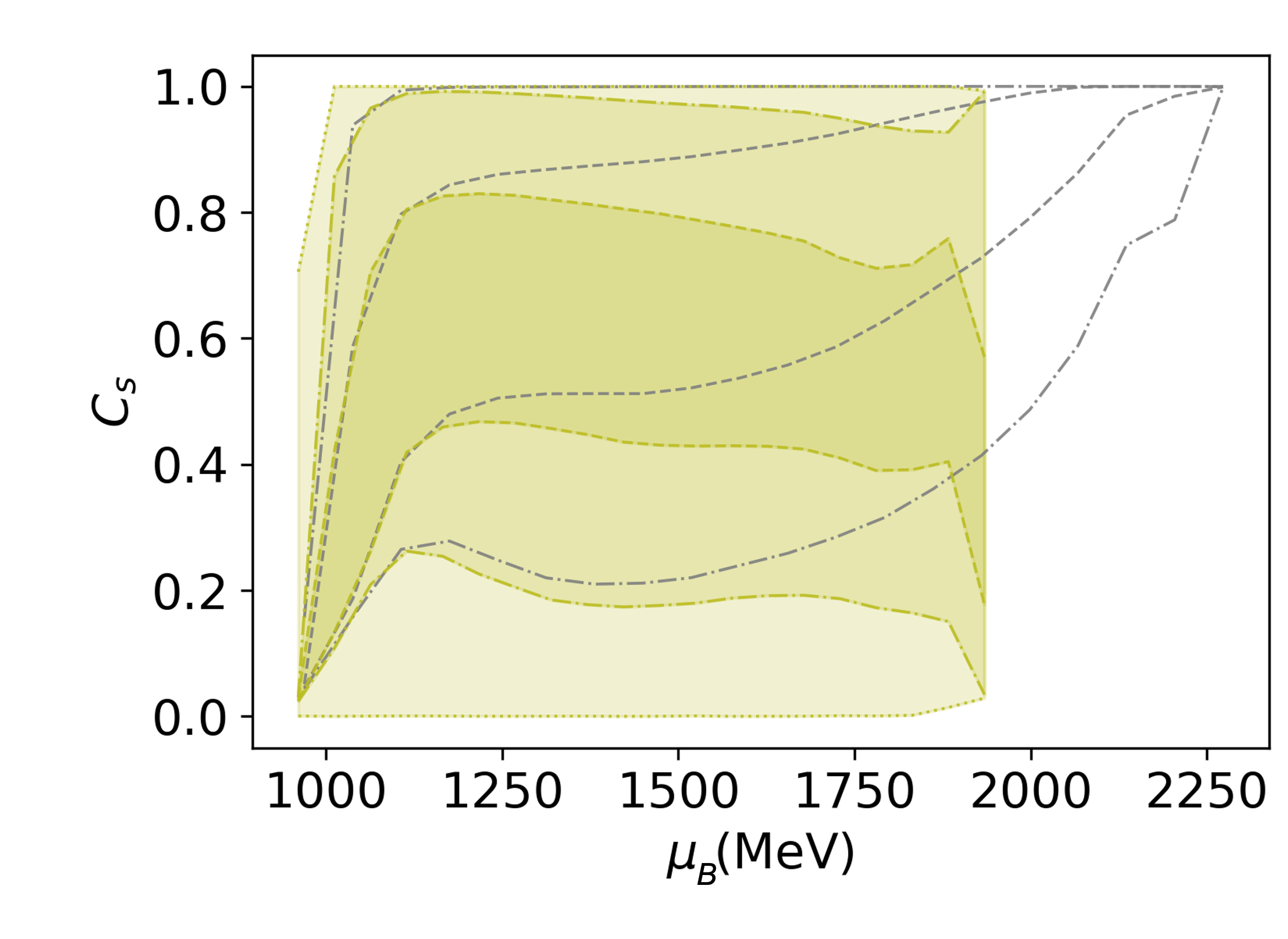
Figure 7: The prior and posterior of the speed of sound squared $C_{s}$ for the PQCD constraint in fig. 6. The yellow dashed, dash-dotted, and dotted lines are the $50\%$, $90\%$, and $100\%$ posterior CIs respectively, whereas the gray lines show the $50\%$ and $90\%$ priors. The prior appears to be biased toward larger $C_{s}$, but this is a consequence of truncating each EOS at its TOV point, and only EOSs with larger $C_{s}$ predict higher $\mu_{\text{TOV}}$ (see main text). That the prior is indeed flat can be seen in fig. 11. This drastic shift in the poster CIs here appears to be the strongest effect the PQCD constraint eq. 11 might impart to NS EOSs.

While the astrophysical observables are not affected by the PQCD constraints, the alteration described above does suggest that the PQCD constraint favors low values of the speed of sound squared $C_{s}$ near the TOV point. This preference is shown in fig. 7, where the posteriors on $C_{s}$ are shifted downwards by the aforementioned PQCD constraint, an increasingly noticeable effect towards higher baryon chemical potentials. In appendix C we shall show that this shift is almost orthogonal to constraints expected from astrophysical observations.

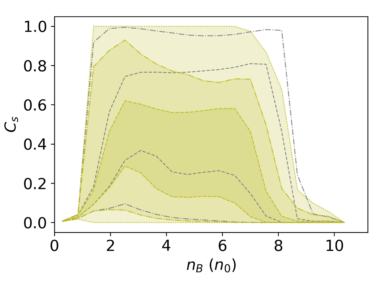
Figure 11: Same as fig. 7 except plotted in the $n_{B}-C_{s}$ plane. Notice that the prior CIs shown in black are centered around $0.5$ and mostly flat, confirming the peculiar shape seen in fig. 7 is a feature of solutions to the TOV equation instead of an indication of bias. Since the PQCD constraint directly impacts $C_{s}(\mu_{B})$, its effects here can be somewhat sensitive to the assumptions underlying the NS EOSs. The results shown here, which drive the CIs lower without introducing additional features, appear to be general and insensitive to those assumptions.

It is quite remarkable that the PQCD constraint effectively rules out $\mu_{\text{TOV}}\gtrsim 1.9$ GeV in the posterior in fig. 7. This is not surprising given that even the maximally soft EOSs, whose predictions for $P_{\text{TOV}}$ are the highest possible, are excluded in fig. 5 if $X\gtrsim 1.6$. In other words, the bound eq. 11 demonstrates higher sensitivity toward $\mu_{\text{TOV}}$ over $P_{\text{TOV}}$, in the sense that an NS EOS is more likely in tension with PQCD if it accommodates higher $\mu_{\text{TOV}}$, almost regardless of its prediction for $P_{\text{TOV}}$, as compared with those predict lower values of $\mu_{\text{TOV}}$. For example, for matching done at $\mu_{\text{pQCD}}=2.4$ GeV, all of the NS EOSs excluded by eq. 11 predict $\mu_{\text{TOV}}\gtrsim 1.8$ GeV. This observation helps establish a simple criterion. While none of the astrophysical observables appear to correlate with $\mu_{\text{TOV}}$, the maximum speed of sound squared $C_{s,\mathrm{max}}$ of an NS EOS is a reliable predictor of $\mu_{\text{TOV}}$. Assuming $\chi$EFT is valid up to $n_{\text{$\chi$EFT}}=n_{0}$ (2$n_{0}$), $C_{s,\mathrm{max}}$ needs to exceed $\sim$ 0.6 (0.5) in order that $\mu_{\text{TOV}}\gtrsim 1.8$ GeV. This correlation also explains the seemingly biased sample selections shown in fig. 7: the prior on $C_{s}$ favors increasingly high values of $C_{s}$ with increasing $\mu_{B}$ because only EOSs with larger $C_{s,\mathrm{max}}$ would lead to higher $\mu_{\text{TOV}}$, and if the EOSs are not truncated at their respective TOV points the prior would be mostly flat and featureless. The CIs plotted against number densities shown in fig. 11 also corroborate this. This dependence of $\mu_{\text{TOV}}$ on $C_{s,\mathrm{max}}$ can be understood by considering the simple constant $C_{s}$ inner core EOS after $n_{\text{$\chi$EFT}}$. The upshot is that an NS EOS would not violate the PQCD constraint if it has $C_{s,\mathrm{max}}\lesssim 0.6$. We note that this is only a necessary condition, and that $C_{s,\mathrm{max}}\gtrsim 0.6$ does not automatically lead to the violation of eq. 11.

So far we have focused on the most optimistic scenarios where the matching to PQCD is performed at $\mu_{\text{pQCD}}=2.4$ GeV, and have focused on $X=4$ which predicts the largest value of $P_{\text{pQCD}}$. The constraining power of PQCD EOSs decreases drastically as the matching point is raised. For eq. 11 imposed at $\mu_{\text{pQCD}}=2.6$ GeV, only NS EOSs with $C_{s,\mathrm{max}}=0.75$ can potentially be ruled out, a condition tightens to $C_{s,\mathrm{max}}\gtrsim 0.9$ for matching performed at $\mu_{\text{pQCD}}=2.8$ GeV. If the matching is done above $\sim 2.9$ GeV, eq. 11 becomes completely irrelevant. Furthermore, lowering the renormalization scale $X$ also limits the potential of such constraints. At $X=1$, no NS EOS that supports $2\mathrm{M_{\odot}}$ can be ruled out.

To account for the uncertainties associated with $X$, we perform a simple inference by noting that while PQCD predictions for $P_{\text{pQCD}}$ are huge, the uncertainties for number densities are controlled. We therefore fix $n_{\text{pQCD}}$ to the fiducial value $5~{}\text{fm}^{-3}$, but sample $P_{\text{pQCD}}$ randomly from a uniform (and log-uniform) distribution on $[0.5,3]$ GeV/fm³, the predicted range at $\mu_{\text{pQCD}}=2.4$ GeV. Analysis in fig. 7 is then repeated but uses this mocked set of $P_{\text{pQCD}}$ instead. Unsurprisingly, the posteriors on $C_{s}$ are almost identical to the priors even for $\mu_{B}\gtrsim 2.0$, a result independent of values of $\mu_{\text{pQCD}}$, whether or not varying $n_{\text{pQCD}}$, or if the N3LO contributions are included (appendix B), or raising $n_{\text{$\chi$EFT}}$ . Since the constraints on $C_{s}(\mu_{B})$ appear to be the strongest, it is safe to conclude that the current untamed uncertainties of PQCD EOSs make it impossible to place meaningful constraints on NS EOSs.

We conclude with cautious optimism by providing a forecast on the presumption that $P_{\text{pQCD}}$ at 2.4 GeV will be reliably obtained. For $P_{\text{pQCD}}(2.4~{}\text{GeV})=3$ GeV/fm³, the expectation value for the speed of sound squared at the center of TOV stars, $C_{s,\text{TOV}}$, is expected to be lowered by up to 0.2-0.3 by eq. 11, whereas for $P_{\text{pQCD}}(2.4~{}\text{GeV})=2$ GeV/fm³ the anticipated effect drops to about 0.1-0.2, and would be less than $\sim 0.05$ if $P_{\text{pQCD}}(2.4~{}\text{GeV})=1.5$ GeV/fm³, an effect hardly distinguishable from that due to implicit assumptions in the underlying NS EOSs. Again, these forecasted bounds are almost orthogonal to those expected from astrophysical observations, unless highly specific features are assumed for NS EOSs (see e.g., appendix C, [20]).

V.3 eq. 11 is the necessary and sufficient condition

As noted above, compliance of eq. 11 for $\mu_{L}=\mu_{\text{TOV}}$ is the sufficient condition for a given EOS satisfying the PQCD constraint, and ensuring it holds for all $\mu_{L}<\mu_{\text{TOV}}$ is the necessary condition. It follows that from a practical point of view, one only needs to check eq. 11 at the TOV point of an EOS to determine if the constraint applies. Discussions on the critical point $\mu_{\mathrm{crit}}<\mu_{\text{TOV}}$ only serve to clarify the constraining power of PQCD, and are not necessary in general.

Recently, a so-called integral constraint is proposed in [18]. It is yet another and one of many necessary conditions one may conceive. It is equivalent to the necessary condition discussed above and is formulated in the $\mu_{B}-n_{B}$ plane, although the way it has been applied is only approximate, as the (comparatively controlled and less important) uncertainties associated with $\chi$EFT  are ignored. Even though this constraint on number density does not reveal new information beyond what is encoded in eq. 11, for the sake of completeness, we discuss it in appendix D.

VI discussion and conclusion

Aided by thermodynamic consistency requirements the high-density PQCD calculations may place bounds on the pressure of an NS EOS if it predicts a chemical potential at the TOV point higher than $\sim 1.8$ GeV. The larger $\mu_{\text{TOV}}$, the tighter the constraint becomes. If the pressure of the NS EOS is too high, the absence of a valid construction between $\mu_{\text{TOV}}$ and $\mu_{\text{pQCD}}$ could indicate the presence of non-perturbative effects, and that unpaired quark matter described by the PQCD EOS is likely not the true ground state around $\mu_{B}\lesssim 3$ GeV. This is not a constraint on NS EOSs, at least not yet.

On the other hand, an EOS may be incompatible with given PQCD EOSs if its predictions for the pressure are too low to reach $P_{\text{pQCD}}$ at $\mu_{\text{pQCD}}$. This is the $\Delta P_{\max}$ bound eq. 11, and is the sole requirement an EOS needs to comply with. Constraints of this type only concern densities that are relevant for stars very close to their respective TOV limits ($M_{\text{TOV}}-M_{\mathrm{crit}}$ no more than $0.06M_{\odot}$ for $M_{\text{TOV}}=4M_{\odot}$, a bound decreases with decreasing $M_{\text{TOV}}$), therefore do not affect observables for most NSs. The strongest possible PQCD constraint (at $\mu_{\text{pQCD}}=2.4$ GeV, assuming $X=4$ and including N3LO soft contributions that push $P_{\text{pQCD}}$ higher) can at best rule out $R_{\text{TOV}}\lesssim 9.5$ km, or compactness of TOV stars $C_{\text{TOV}}=M_{\text{TOV}}/R_{\text{TOV}}\gtrsim 0.33$, assuming $\chi$EFT  is valid up to $n_{0}$. Even if the two-solar mass pulsars observed to date are in fact the TOV limit, such constraints would only raise the expectation value of $R_{2\mathrm{M_{\odot}}}$ by no more than $0.2$ km. Accounting for the uncertainties of PQCD requires choosing a prior on PQCD EOSs. With natural choices of priors no meaningful bounds can be derived at the moment owning to the wild uncertainties associated with PQCD EOSs.

Although the bound eq. 11 directly constrains the pressure of NS EOSs, it is more sensitive to $\mu_{\text{TOV}}$, as even the highest pressure predicted by the maximally soft NS EOS at $\mu_{\text{TOV}}\gtrsim 2$ GeV is too low to reach $P_{\text{pQCD}}$ for $X\gtrsim 2$. Any NS EOS predicting $\mu_{\text{TOV}}\gtrsim 1.8$ GeV is at risk of being ruled out by such considerations. The necessary condition for supporting high values of $\mu_{\text{TOV}}$ is large $C_{s,\mathrm{max}}\gtrsim 0.5$ of NS EOSs.

Non-perturbative effects are not expected to drastically impact the PQCD constraint. The reason is that those constraining PQCD EOSs already predict high pressure $P_{\text{pQCD}}\gtrsim 2$ GeV/fm³ in the density range of interest, so the effect of a typical pairing gap $\Delta\sim 100$ MeV

$$P_{\mathrm{CFL}}=\frac{3\Delta^{2}\mu_{q}^{2}}{\pi^{2}}\simeq 0.3\mathrm{GeV/fm}^{3}~{}\left(\frac{\Delta}{100~{}\text{MeV}}\right)\left(\frac{\mu_{q}}{800~{}\text{MeV}}\right)^{2}$$ (12)

would be moderate. However, if PQCD predictions of pressures are indeed low and fall in the vicinity of current predictions near $X=1$, astrophysical evidence for soft NS EOSs would likely indicate the presence of exotic phases such as a CFL color superconductor beyond neutron star densities. The constraint also appears to be insensitive to the mass of strange quarks $m_{s}$. In the decoupling limit $m_{s}\rightarrow\infty$, the 2-flavor quark matter EOS only differs by about $~{}20\%$ at $\mu_{B}\sim 2.6$ GeV, moving the bands in fig. 7 by no more than $\sim 10\%$.

Recently, ref [18] reported another necessary condition. As discussed above and detailed in appendix D, this necessary condition does not lead to additional constraints beyond eq. 11. By matching neutron star EOS at a fixed density $n_{B}\sim 10n_{0}$, that letter and the following works excluded large numbers of EOSs based on densities that are not probed in the interior of stable neutron stars. This is especially problematic for stiff EOSs as their predictions for $n_{\text{TOV}}\lesssim 4n_{0}$ and for $P(n_{B}>n_{\text{TOV}})$ are typically low. Ref  [19] correctly addressed this issue, but arrived at the misleading if not incorrect conclusion that PQCD is not constraining if imposed on top of current astrophysical observations. As discussed earlier, PQCD constraints are only relevant for stars very close to the TOV limit so would not affect observables appreciably, but they yield constraints on EOSs that are mostly orthogonal to those from observations. Finally, their claim regarding the possible interplay between PQCD constraints and $R\gtrsim 13$ km is likely due to bias in their parameterization of inner core EOSs, which is an approximation to a subset of the ensembles in this work. Addressing implicit assumptions in the parameterizations of NS EOSs is important and is relevant for a wider range of issues but requires a much much lengthier discussion and will be reported in a separate work [20].

Improving the uncertainties of the cold quark matter EOS is crucial in materializing the potentials demonstrated by constraints of this type. As noted earlier, although typically referred to as the renormalization scale uncertainties, it is a form of truncation error in disguise, as the dependency on $X$ is an artifact that is expected to receive cancellations when higher order terms become known. This is shown to be the case in dense QED [37] and hot QCD calculations [38, 39], and one could expect it to hold in dense QCD as well assuming PQCD is a valid description. Effort employing strategies developed in $\chi$EFT [21] to understand better PQCD truncation errors is underway and will be reported in a future work.

This work confirms and strengthens previous findings that the knowledge of neutron star global properties alone may not be adequate to distinguish the relevant microscopic degrees of freedom inside the cores of NSs [51]. Although it is possible for extreme cases of PQCD EOSs to place upper bounds on the speed of sound above $\mu_{B}\gtrsim 2$ GeV, we caution against interpreting this as evidence for quark matter, as extrapolating $C_{s}$ from PQCD predictions above $\sim 2.5~{}\text{GeV}$ to such low densities could be unwarranted as non-perturbative effects may still dominate. Understanding the QCD phase diagram in this intermediate density range is inherently challenging, as neither PQCD nor NSs directly probe this regime.

Appendix A the running of $\alpha_{s}$

We give a brief overview of the uncertainties associated with $\alpha_{s}\equiv g_{s}^{2}/(4\pi)^{2}$ around $\sim$ GeV scales. To obtain the strong coupling constant at a given scale $\bar{\Lambda}$ we solve the renormalization group equation

$$\frac{\mathrm{d}\alpha_{s}}{\mathrm{d}\log\bar{\Lambda}^{2}}=-\sum_{i\geq 0}\frac{\beta_{i}}{(4\pi)^{i+1}}\alpha_{s}^{i+2}=-\sum_{i\geq 0}b_{i}\alpha_{s}^{i+2}$$ (13)

up to 2, 3, 4 and 5 loops. For $N_{c}=3$ QCD with $N_{f}$ active flavors of quarks the beta function coefficients are given by [52]

$$\beta_{0} =11-\frac{2N_{f}}{3},$$ (14)

$$\beta_{1} =102-\frac{38N_{f}}{3},$$ (15)

$$\beta_{2} =\frac{325N_{f}^{2}}{54}-\frac{5033N_{f}}{18}+\frac{2857}{2},$$ (16)

$$\beta_{3} =\frac{149753}{6}+3564\zeta_{3}-\left(\frac{1078361}{162}+\frac{6508}{27}\zeta_{3}\right)N_{f}+\left(\frac{50065}{162}+\frac{6472}{81}\zeta_{3}\right)N_{f}^{2}+\frac{1093}{729}N_{f}^{3},$$ (17)

$$\begin{split}\beta_{4}&=\frac{8157455}{16}+\frac{621885}{2}\zeta_{3}-\frac{88209}{2}\zeta_{4}-288090\zeta_{5}+\left(-\frac{336460813}{1944}-\frac{4811164}{81}\zeta_{3}+\frac{33935}{6}\zeta_{4}+\frac{1358995}{27}\zeta_{5}\right)N_{f}\\ {}&+\left(\frac{25960913}{1944}+\frac{98531}{81}\zeta_{3}-\frac{10526}{9}\zeta_{4}-\frac{381760}{81}\zeta_{5}\right)N_{f}^{2}\\ {}&+\left(-\frac{630559}{5832}-\frac{48722}{243}\zeta_{3}+\frac{1618}{27}\zeta_{4}+\frac{460}{9}\zeta_{5}\right)N_{f}^{3}+\left(\frac{1205}{2916}-\frac{152}{81}\zeta_{3}\right)N_{f}^{4},\end{split}$$ (18)

where $\zeta_{n}\equiv\zeta(n)$ are values of the Riemann zeta function. Coefficients beyond 2 loop ($\beta_{1}$) are renormalization scheme dependent, and the values quoted above are given in $\overline{\mathrm{MS}}$. Equation 13 can be solved either numerically, or analytically albeit approximately in a perturbative fashion. Defining $t=2\log(\bar{\Lambda}/\bar{\Lambda}_{\overline{\mathrm{MS}}})$ and $l=\log(t)$, an iterative solution to the 5-loop renormalization group equation ($\mathcal{O}(\alpha_{s}^{6})$ on the right hand side of eq. 13) is given by

$$\alpha_{s}(\bar{\Lambda}^{2})=\frac{1}{b_{0}t}\left[1-\frac{b_{1}l}{b_{0}^{2}t}+\frac{b_{1}^{2}\left(l^{2}-l-1\right)+b_{0}b_{2}}{b_{0}^{4}t^{2}}+\frac{b_{1}^{3}\left(-2l^{3}+5l^{2}+4l-1\right)-6b_{0}b_{1}b_{2}l+b_{0}^{2}b_{3}}{2b_{0}^{6}t^{3}}\right.\\ \left.+\frac{18b_{0}b_{2}b_{1}^{2}\left(2l^{2}-l-1\right)+b_{1}^{4}\left(6l^{4}-26l^{3}-9l^{2}+24l+7\right)+2b_{0}^{2}\left(5b_{2}^{2}+b_{0}b_{4}\right)-b_{0}^{2}b_{1}b_{3}(12l+1)}{6b_{0}^{8}t^{4}}\right].$$ (19)

Its exact derivatives up to the second order are

$$\frac{\mathrm{d}\alpha_{s}(\bar{\Lambda}^{2})}{\mathrm{d}\log\bar{\Lambda}^{2}}=-\frac{1}{b_{0}t^{2}}\left[1+\frac{b_{1}(1-2l)}{b_{0}^{2}t}+\frac{b_{1}^{2}(-2-5l+3l^{2})+3b_{0}b_{2}}{b_{0}^{4}t^{2}}\right.\\ +\frac{b_{1}^{3}(-4+3l+13l^{2}-4l^{3})+3b_{0}b_{2}b_{1}(1-4l)+2b_{0}^{2}b_{3}}{b_{0}^{6}t^{3}}\\ \left.+\frac{b_{1}^{4}(11+138l+33l^{2}-154l^{3}+30l^{4})+18b_{0}b_{2}b_{1}^{2}(-4-9l+10l^{2})+b_{0}^{2}b_{3}b_{1}(7-60l)+10b_{0}^{2}\left(5b_{2}^{2}+b_{0}b_{4}\right)}{6b_{0}^{8}t^{4}}\right],$$ (20)

$$\frac{\mathrm{d}^{2}\alpha_{s}(\bar{\Lambda}^{2})}{\mathrm{d}\left(\log\bar{\Lambda}^{2}\right)^{2}}=\frac{2}{b_{0}t^{3}}\left[1+\frac{b_{1}(5-6l)}{2b_{0}^{2}t}+\frac{b_{1}^{2}(-3-26l+12l^{2})+12b_{0}b_{2}}{2b_{0}^{4}t^{2}}\right.\\ +\frac{-b_{1}^{3}(23+11l-77l^{2}+20l^{3})+3b_{0}b_{2}b_{1}(9-20l)+10b_{0}^{2}b_{3}}{2b_{0}^{6}t^{3}}\\ \left.+\frac{3b_{0}b_{2}b_{1}^{2}\left(60l^{2}-74l-15\right)+b_{1}^{4}(127l+110l^{2}-174l^{3}+30l^{4})+b_{0}^{2}b_{3}b_{1}(17-60l)+10b_{0}^{2}\left(5b_{2}^{2}+b_{0}b_{4}\right)}{2b_{0}^{8}t^{4}}\right].$$ (21)

We do not use the renormalization group equation eq. 13 to compute the derivatives as eq. 19 is only an approximate solution to the 5-loop renormalization group equation. The residue, although small, would spoil the thermodynamic consistency of the PQCD EOS if eq. 13 were to used in calculating $n_{B}=\frac{\mathrm{d}P}{\mathrm{d}\mu_{B}}$ and $C_{s}=\mathrm{d}\log\mu_{B}/\mathrm{d}\log n_{B}$.

The 2-, 3-, 4-loop solutions of $\alpha_{s}$ can be obtained by setting $b_{i>n_{\mathrm{loop}}-1}=0$ where $n_{\mathrm{loop}}=2,3,4$. It is also customary, although not necessary, to truncate the iterative solutions in eq. 19 at order $\left(\frac{b_{i}}{b_{0}^{2}}\right)^{n_{\mathrm{loop}}-1}$ in the literature, i.e., only keep the leading power in $b_{n_{\mathrm{loop}}-1}$. We also adopt this convention throughout this paper.

The Landau pole $\bar{\Lambda}_{\overline{\mathrm{MS}}}$ is determined once the strong coupling at a given reference scale is specified. Above, we took the value $\alpha_{s}(\bar{\Lambda}=2~{}\text{GeV})=0.2994^{+0.0152}_{-0.0141}$ from the 2008 particle data group (PDG) report. The resulting $P_{\text{pQCD}}$ and its uncertainties at $\mu_{B}=2.4$ GeV are shown in fig. 8. Since then, PDG only reports $\alpha_{s}(\bar{\Lambda}=M_{Z})$. Running $\alpha_{s}$ from the Z boson mass $M_{Z}\sim 100\text{GeV}$ to GeV scales is not straightforward as the decoupling of both charm and bottom quarks occurs in this regime. But because the uncertainties of $\alpha_{s}(M_{Z})$ are barely reduced since 2008, we do not expect significant improvements for the bound on $\alpha_{s}(2~{}\text{GeV})$ quoted above. Furthermore, the current inferred values of $\alpha_{s}(M_{Z})$ could suffer from non-negligible modeling uncertainties as a few subsets of measurements behind the PDG averaged value appear to be in disagreement [53]. A careful running of $\alpha_{s}$ from $M_{Z}$ where $N_{f}=5$ to $\sim\text{GeV}$ scales where $N_{f}=3$ will be performed in a future work.

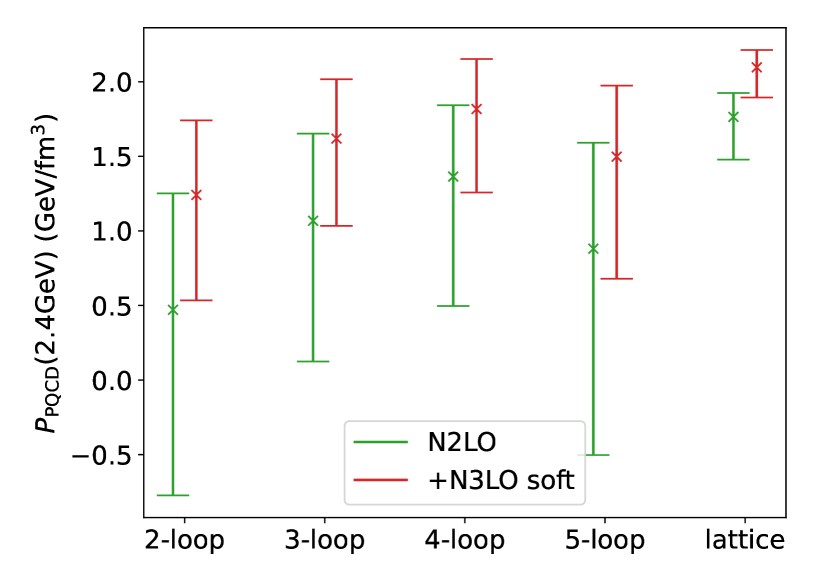
Figure 8: Pressure of the PQCD EOS with $X=1$ at $\mu_{B}=2.4$ GeV obtained with 2-, 3-, 4-, and 5-loop QCD beta functions. The central values and error bars correspond to those of the reference value $\alpha_{s}(\bar{\Lambda}=2~{}\text{GeV})=0.2994^{+0.0152}_{-0.0141}$. The last column labeled “lattice” uses the extracted Landau pole from lattice data [54] and is obtained with a 4-loop running (see main text). The 2-loop $\alpha_{s}$ adopted in the main text leads to the largest uncertainties, but is consistent with the N2LO PQCD calculation eq. 3. Notice that the effect of the N3LO soft contribution can be significant, and in most cases appear to improve the convergence of PQCD.

An alternative approach is to take the values of Landau pole $\bar{\Lambda}_{\overline{\mathrm{MS}}}$ reported in the literature. This is generally disfavored as these values can be quite sensitive to the order of renormalization group equations used in the analysis. For instance, in fig. 8 the underlying $\bar{\Lambda}_{\overline{\mathrm{MS}}}$ ranges from $\sim 310$ to $\sim 390$ MeV. In [54] the authors matched lattice data for the static $q\bar{q}$ potential to a resummed next-to-next-to-next-leading log perturbative calculation in the perturbative regime $\sim 5~{}\text{GeV}$ and obtained $\bar{\Lambda}_{\overline{\mathrm{MS}}}=315^{+18}_{-12}~{}\text{MeV}$. PQCD EOS based on this value is shown as the last column in fig. 8 and is labeled as “lattice”, where we assumed a 4-loop running $\alpha_{s}$ that is used throughout [54]. It is not clear if some of the choices are better than others.

Appendix B the partial N3LO PQCD EOS

The partial N3LO contribution to the PQCD EOS recently reported in [15, 17] pushes the pressure higher than that predicted by the N2LO result eq. 3, as can be seen in fig. 8. Although this makes eq. 11 more constraining, the main conclusions remain unchanged. For instance, as is shown in fig. 9, the maximally stiff EOSs are still compatible with PQCD predictions assuming $X=1$. Since the maximally stiff inner core EOS predicts the lowest pressure at $\mu_{B}\sim 2.2\text{GeV}$, no other valid NS EOSs can be ruled out either.

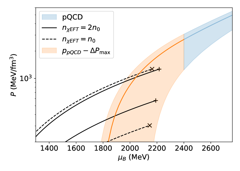
Figure 9: Similar to fig. 5 except that the partial N3LO contribution is included in the PQCD EOS. None of the NS EOSs are completely ruled out.

Appendix C imposing astrophysical constraints

We have shown in the main text with both limiting scenarios and with randomly generated samples that (potential) PQCD bounds are orthogonal to those from astrophysical observations. Here we strengthen this statement by explicitly taking into account astrophysical constraints. Specifically, we impose the tentative bounds on the tidal deformability of $1.4\mathrm{M_{\odot}}$ stars $\Lambda_{1.4\mathrm{M_{\odot}}}\leq 500$ from GW170817 [55, 56, 57], and the putative upper limit $M_{\text{TOV}}\lesssim 2.3$ based on the speculation that the remnant of GW170817 collapsed to a black hole within seconds [58, 59]. That the former is orthogonal to PQCD considerations is demonstrated earlier in fig. 6, and that the latter might interfere with PQCD constraints is mainly due to the closer proximity of the TOV limit to $2\mathrm{M_{\odot}}$ stars. However, we do not find any appreciable changes in the observables of $2\mathrm{M_{\odot}}$ stars. The same observation holds for the posterior CIs of $C_{s}(\mu_{B})$ (see fig. 13) where the effects of PQCD considerations are the most evident.

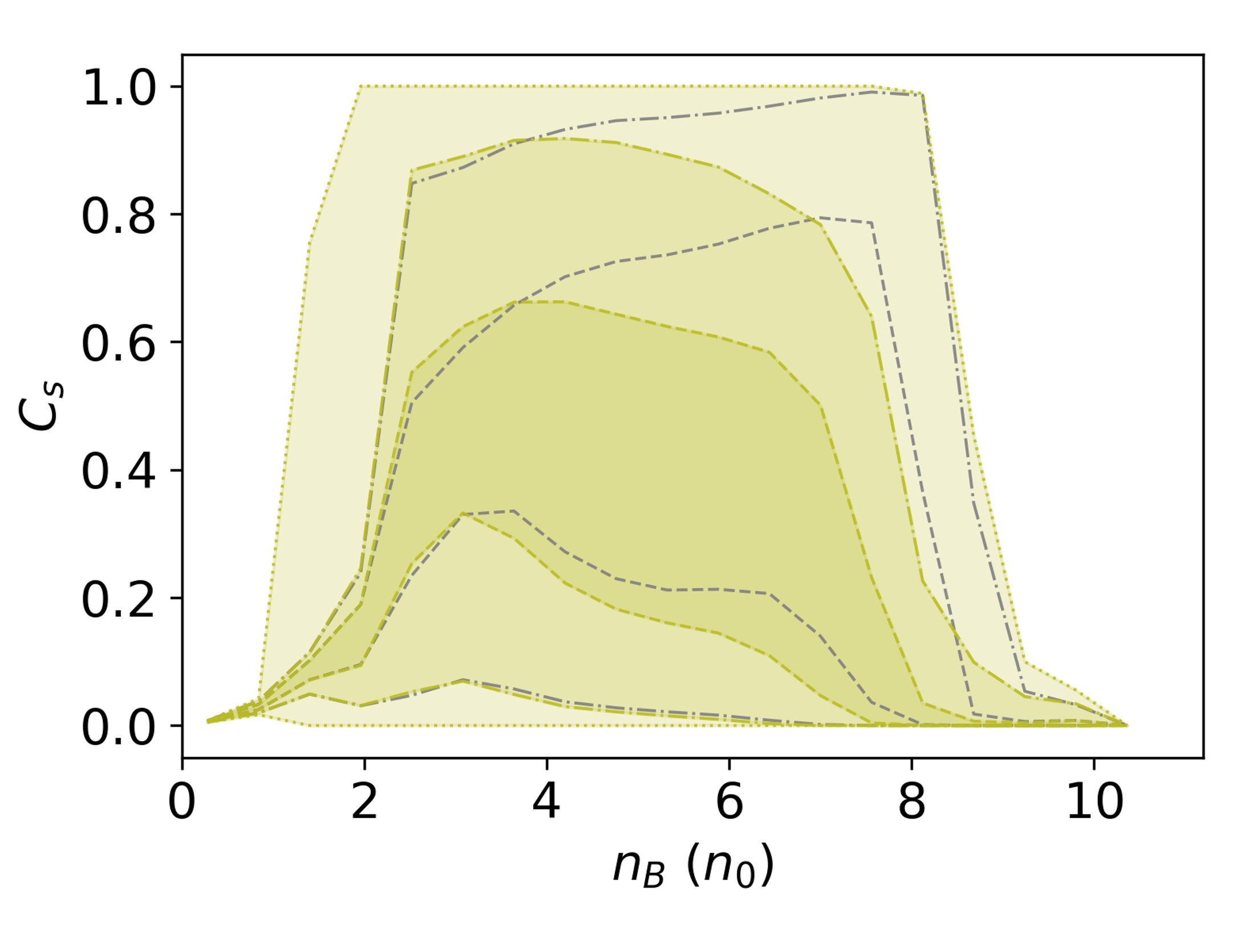
Figure 12: Similar to fig. 11 except that the astrophysical bounds $\Lambda_{1.4\mathrm{M_{\odot}}}\leq 500$ and $M_{\text{TOV}}\leq 2.3\mathrm{M_{\odot}}$ are implied in the prior.

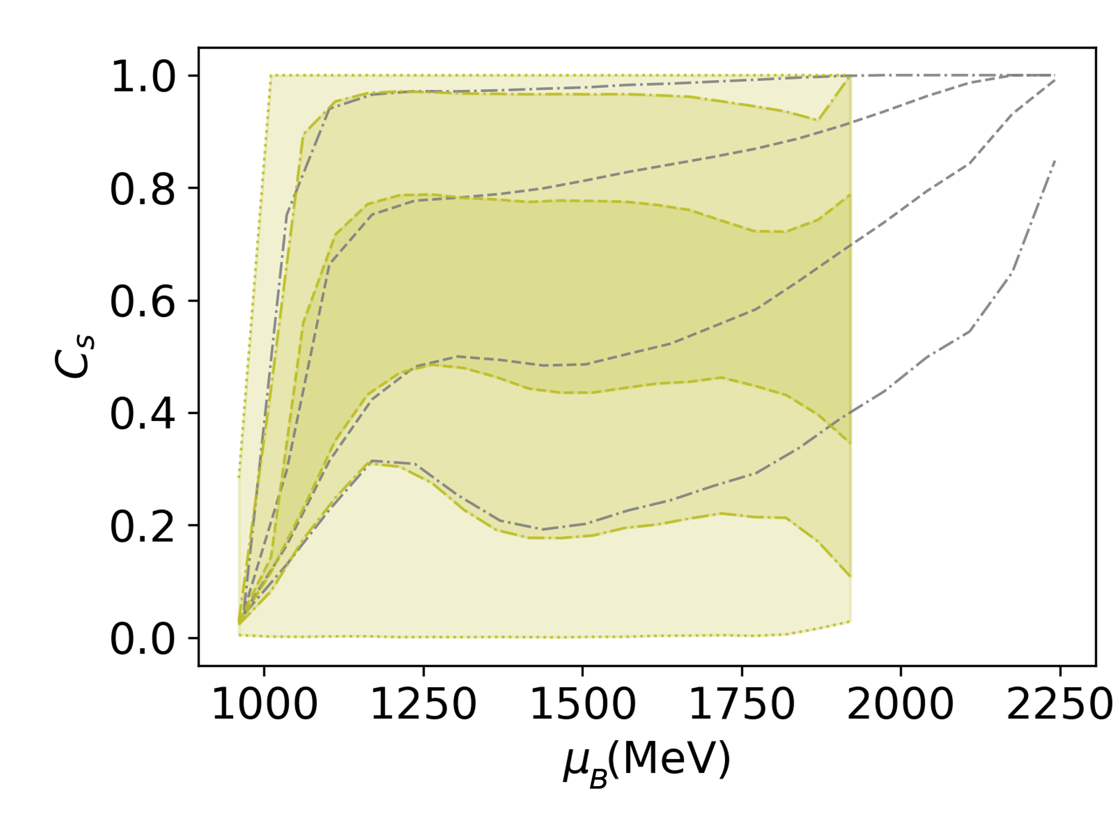
Figure 13: Same as fig. 7, but assumes a prior that already incorporates astrophysical constraints $\Lambda_{1.4\mathrm{M_{\odot}}}\leq 500$ and $M_{\text{TOV}}\leq 2.3\mathrm{M_{\odot}}$. When compared to fig. 7 we see that the astrophysical inputs have negligible effects on $C_{s}(\mu_{B})$, even in this hard cutoff approach ignoring astrophysical uncertainties. The PQCD bound once again shifts the CIs on $C_{s}$ towards lower values, and forbids $\mu_{\text{TOV}}$ above $\sim 1.9$ GeV.

Appendix D the number density constraint

The low-density matching points in the $\Delta P_{\mathrm{min}}$ and $\Delta P_{\mathrm{max}}$ bounds are taken to be at or below the TOV points of NS EOSs, which vary from one EOS to another. The number density constraint derived in [18] is in a sense a global bound that concerns fixed low- and high-density matching points L and H. We will take the low- and high-density matching points to be $\mu_{\text{$\chi$EFT}}$ and $\mu_{\text{pQCD}}$. For all EOSs that pass through an arbitrary point $(\mu_{1},n_{1})$ between the two endpoints there exist a maximum and a minimum value of $\Delta P$. These limiting cases are shown as the blue and the red curves in fig. 14. By noting the constructions in the density ranges $[\mu_{L},\mu_{1}]$ and $[\mu_{1},\mu_{H}]$ are two separate realizations of fig. 3, the expressions for $\Delta P_{\mathrm{min}}$ and $\Delta P_{\mathrm{max}}$ can be obtained by replacing the dummy labels in eqs. 8 and 9, and are

$$\Delta P_{\mathrm{max}} =\frac{n_{H}\mu_{H}}{2}\left[1-\left(\frac{\mu_{1}}{\mu_{H}}\right)^{2}\right]+\frac{n_{1}\mu_{1}}{2}\left[1-\left(\frac{\mu_{L}}{\mu_{1}}\right)^{2}\right],$$ (22)

$$\Delta P_{\mathrm{min}} =\frac{n_{L}\mu_{L}}{2}\left[\left(\frac{\mu_{1}}{\mu_{L}}\right)^{2}-1\right]+\frac{n_{1}\mu_{1}}{2}\left[\left(\frac{\mu_{H}}{\mu_{1}}\right)^{2}-1\right].$$ (23)

In order that there exists an EOS passing through $(\mu_{1},n_{1})$, $\Delta P_{0}\equiv P_{H}-P_{L}$ has to be sandwiched by these limits $\Delta P_{\mathrm{min}}\leq\Delta P_{0}\leq\Delta P_{\mathrm{max}}$. But as discussed earlier, only the $\Delta P_{\mathrm{max}}$ bound may be used as a constraint, and it leads to the number density constraint $n_{1}(\mu_{1})\geq n_{\mathrm{min}}(\mu_{1})$ where

$$n_{\mathrm{min}}(\mu)=\frac{2\Delta P_{0}-\mu_{H}n_{H}\left[1-\left(\frac{\mu}{\mu_{H}}\right)^{2}\right]}{\mu\left[1-\left(\frac{\mu_{L}}{\mu}\right)^{2}\right]}.$$ (24)

This lower limit can be relevant for large $\mu$ close to $\mu_{H}$, but it blows off near $\mu_{L}$. In fact, it crosses the lower bound eq. 7 (noting that ‘H’ and ‘L’ are just dummy labels there) set by the maximally stiff EOS (blue curve in fig. 14) at

$$\mu_{C}=\sqrt{\mu_{L}\mu_{H}\frac{\mu_{L}n_{L}-\mu_{H}n_{H}+2\Delta P_{0}}{\mu_{H}n_{L}-\mu_{L}n_{H}}}.$$ (25)

Therefore, for baryon chemical potentials below this value $\mu_{C}$, eq. 7

$$n_{\mathrm{min}}(\mu)=\frac{\mu}{\mu_{L}}n_{L}$$ (26)

is the relevant bound.

The $n_{\mathrm{min}}$ bound is shown in fig. 15 as the dashed, dot-dashed, and dotted lines for $X=1,2,4$. The high-density PQCD point is taken to be $\mu_{H}=2.4$ GeV, and we have included the PQCD N3LO leading log term. To compare this necessary condition with the one from eq. 11, we show a few modified NS EOSs described in the main text as solid lines. These are based on the maximally stiff and maximally soft EOSs in fig. 5, and are diverted away at the critical points just before eq. 11 is violated via first-order-phase transitions. These two approaches lead to the same constraint. This equivalence can be understood by noting that $\Delta P_{\mathrm{max}}$ does not depend on $n_{L}$, and the maximally stiff (soft) EOS depicted in blue (red) between $\mu_{L}$ and $\mu_{1}$ is, plainly, the maximally stiff (soft) inner core EOS shown in fig. 15. In other words, any causal and stable NS EOS will automatically satisfy the contributions to $\Delta P_{\mathrm{max}}$ below $\mu_{1}$. This effectively reduces the problem formulated on the interval $[\mu_{L},\mu_{H}]$ to that on $[\mu_{1},\mu_{H}]$, which is exactly fig. 3.

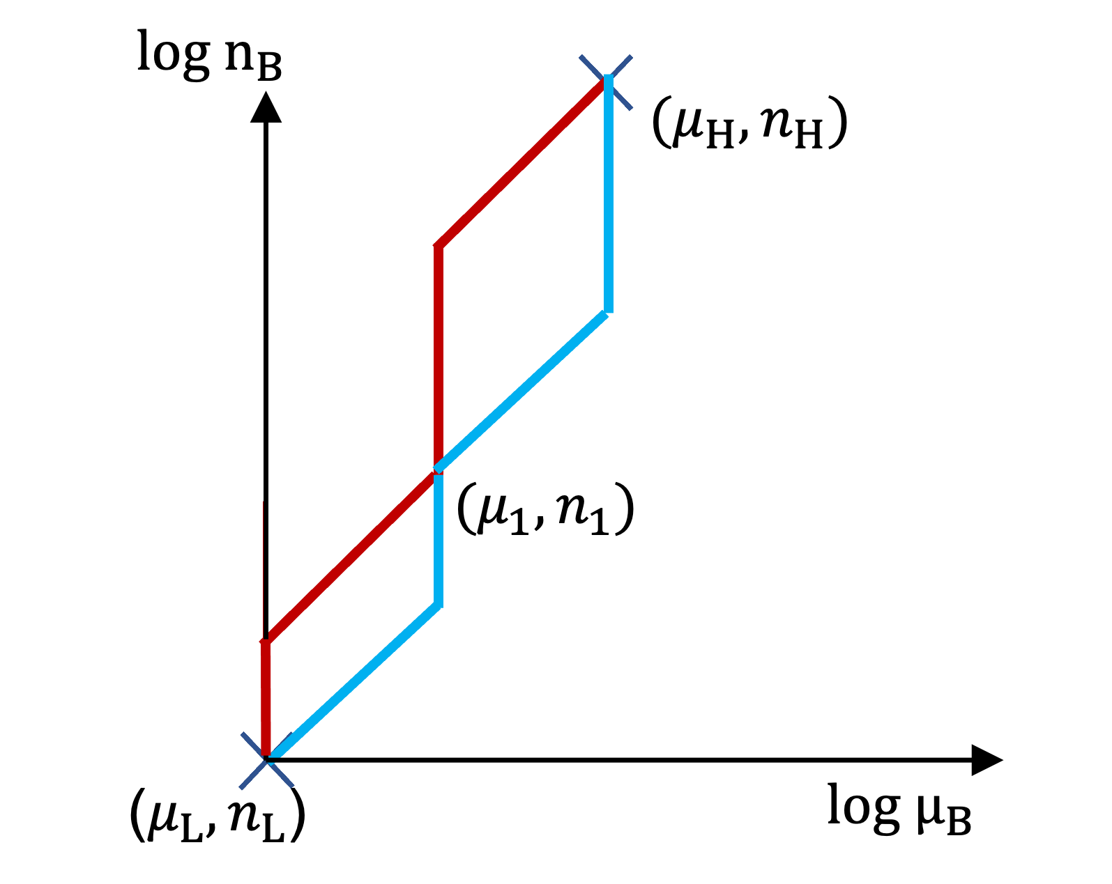
Figure 14: Schematics for the number density constraint for fixed endpoints and $\Delta P_{0}=P(\mu_{H})-P(\mu_{L})$. The curve in blue (red) yields $\Delta P_{\mathrm{min}}$ ($\Delta P_{\mathrm{max}}$) among all possibilities that pass through the point $(\mu_{1},n_{1})$. These constructions are obtained by stacking two copies of fig. 3 on top of each other.

For the sake of completeness, we also provide the expression for $n_{\mathrm{max}}$ derived from $\Delta P_{\mathrm{min}}\leq\Delta P_{0}$:

$$n_{\mathrm{max}}(\mu)=\frac{2\Delta P_{0}-\mu_{L}n_{L}\left[\left(\frac{\mu}{\mu_{L}}\right)^{2}-1\right]}{\mu\left[\left(\frac{\mu_{H}}{\mu}\right)^{2}\right]-1}.$$ (27)

It crosses eq. 6 at $\mu_{C}$ given by eq. 25, above which it is replaced by

$$n_{\mathrm{max}}(\mu)=\frac{\mu}{\mu_{H}}n_{H}.$$

The $n_{\mathrm{max}}$ bound is also shown fig. 15 and appears in the upper regions. It suggests the maximally soft NS EOSs are incompatible with PQCD predictions with $X=1$, and the problem starts early on at $n_{\text{$\chi$EFT}}$ where the first-order phase transitions take place. On one hand, identifying the earliest violation of eq. 10 is a strength of $n_{\mathrm{max}}$. On the other hand, for an intuitive view of the non-perturbative effects required to satisfy eq. 10 (or equivalently the $n_{\mathrm{max}}$ bound), figs. 4 and 10 are better suited.

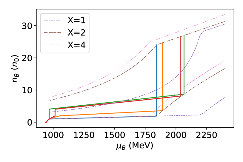
Figure 15: The number density constraints assuming $\mu_{\text{pQCD}}=2.4$ GeV, $X=1,2,4$, $\mu_{L}\approx 970~{}\text{MeV}$ (the central value of $\chi$EFT  prediction at $n_{0}$), and with the partial N3LO contributions included. The colored solid curves are the modified maximally stiff and soft EOSs that are made to be compatible with eq. 11. The modifications are described in the main text and start at the critical points shown in fig. 5. They are obtained assuming the same set of PQCD parameters behind the number density constraints. The critical points sit along the $n_{\mathrm{min}}$ bound, corroborating that the number density constraint is identical to eq. 11 applied at critical points. For the number density constraint as $X=1$, the maximally soft EOSs breach $n_{\mathrm{max}}$ which comes from $\Delta P_{\mathrm{min}}$, and as explained cannot be viewed as a constraint on NS EOSs.

References

- Troyer and Wiese [2005] M. Troyer and U.-J. Wiese, Computational complexity and fundamental limitations to fermionic quantum Monte Carlo simulations, Phys. Rev. Lett. 94, 170201 (2005), arXiv:cond-mat/0408370 .
- de Forcrand [2009] P. de Forcrand, Simulating QCD at finite density, PoS LAT2009, 010 (2009), arXiv:1005.0539 [hep-lat] .
- Kaplan [2009] D. B. Kaplan, Chiral Symmetry and Lattice Fermions, in Les Houches Summer School: Session 93: Modern perspectives in lattice QCD: Quantum field theory and high performance computing (2009) arXiv:0912.2560 [hep-lat] .
- Baade and Zwicky [1934] W. Baade and F. Zwicky, On super-novae, Proceedings of the National Academy of Sciences 20, 254 (1934).
- Weinberg [1991] S. Weinberg, Effective chiral Lagrangians for nucleon - pion interactions and nuclear forces, Nucl. Phys. B 363, 3 (1991).
- Weinberg [1990] S. Weinberg, Nuclear forces from chiral Lagrangians, Phys. Lett. B 251, 288 (1990).
- Kaplan et al. [1996] D. B. Kaplan, M. J. Savage, and M. B. Wise, Nucleon - nucleon scattering from effective field theory, Nucl. Phys. B 478, 629 (1996), arXiv:nucl-th/9605002 .
- Weinberg [1992] S. Weinberg, Three body interactions among nucleons and pions, Phys. Lett. B 295, 114 (1992), arXiv:hep-ph/9209257 .
- Kaplan et al. [1998] D. B. Kaplan, M. J. Savage, and M. B. Wise, A New expansion for nucleon-nucleon interactions, Phys. Lett. B 424, 390 (1998), arXiv:nucl-th/9801034 .
- Drischler et al. [2020] C. Drischler, J. A. Melendez, R. J. Furnstahl, and D. R. Phillips, Quantifying uncertainties and correlations in the nuclear-matter equation of state, Phys. Rev. C 102, 054315 (2020), arXiv:2004.07805 [nucl-th] .
- Freedman and McLerran [1977a] B. A. Freedman and L. D. McLerran, Fermions and Gauge Vector Mesons at Finite Temperature and Density. 1. Formal Techniques, Phys. Rev. D 16, 1130 (1977a).
- Freedman and McLerran [1977b] B. A. Freedman and L. D. McLerran, Fermions and Gauge Vector Mesons at Finite Temperature and Density. 3. The Ground State Energy of a Relativistic Quark Gas, Phys. Rev. D 16, 1169 (1977b).
- Manuel [1996] C. Manuel, Hard dense loops in a cold nonAbelian plasma, Phys. Rev. D 53, 5866 (1996), arXiv:hep-ph/9512365 .
- Kurkela et al. [2010] A. Kurkela, P. Romatschke, and A. Vuorinen, Cold Quark Matter, Phys. Rev. D 81, 105021 (2010), arXiv:0912.1856 [hep-ph] .
- Gorda et al. [2021a] T. Gorda, A. Kurkela, R. Paatelainen, S. Säppi, and A. Vuorinen, Cold quark matter at N3LO: Soft contributions, Phys. Rev. D 104, 074015 (2021a), arXiv:2103.07427 [hep-ph] .
- Kurkela and Vuorinen [2016] A. Kurkela and A. Vuorinen, Cool quark matter, Phys. Rev. Lett. 117, 042501 (2016), arXiv:1603.00750 [hep-ph] .
- Gorda et al. [2018] T. Gorda, A. Kurkela, P. Romatschke, S. Säppi, and A. Vuorinen, Next-to-Next-to-Next-to-Leading Order Pressure of Cold Quark Matter: Leading Logarithm, Phys. Rev. Lett. 121, 202701 (2018), arXiv:1807.04120 [hep-ph] .
- Komoltsev and Kurkela [2022] O. Komoltsev and A. Kurkela, How Perturbative QCD Constrains the Equation of State at Neutron-Star Densities, Phys. Rev. Lett. 128, 202701 (2022), arXiv:2111.05350 [nucl-th] .
- Somasundaram et al. [2023] R. Somasundaram, I. Tews, and J. Margueron, Perturbative QCD and the neutron star equation of state, Phys. Rev. C 107, L052801 (2023), arXiv:2204.14039 [nucl-th] .
- Zhou [2023a] D. Zhou, On the parameterization of neutron star equations of state, in preparation (2023a).
- Melendez et al. [2019] J. A. Melendez, R. J. Furnstahl, D. R. Phillips, M. T. Pratola, and S. Wesolowski, Quantifying Correlated Truncation Errors in Effective Field Theory, Phys. Rev. C 100, 044001 (2019), arXiv:1904.10581 [nucl-th] .
- Drischler et al. [2019] C. Drischler, K. Hebeler, and A. Schwenk, Chiral interactions up to next-to-next-to-next-to-leading order and nuclear saturation, Phys. Rev. Lett. 122, 042501 (2019), arXiv:1710.08220 [nucl-th] .
- Forbes et al. [2019] M. M. Forbes, S. Bose, S. Reddy, D. Zhou, A. Mukherjee, and S. De, Constraining the neutron-matter equation of state with gravitational waves, Phys. Rev. D 100, 083010 (2019), arXiv:1904.04233 [astro-ph.HE] .
- Adhikari et al. [2021] D. Adhikari et al. (PREX), Accurate Determination of the Neutron Skin Thickness of 208Pb through Parity-Violation in Electron Scattering, Phys. Rev. Lett. 126, 172502 (2021), arXiv:2102.10767 [nucl-ex] .
- Reed et al. [2021] B. T. Reed, F. J. Fattoyev, C. J. Horowitz, and J. Piekarewicz, Implications of PREX-2 on the Equation of State of Neutron-Rich Matter, Phys. Rev. Lett. 126, 172503 (2021), arXiv:2101.03193 [nucl-th] .
- McKeen et al. [2018] D. McKeen, A. E. Nelson, S. Reddy, and D. Zhou, Neutron stars exclude light dark baryons, Phys. Rev. Lett. 121, 061802 (2018), arXiv:1802.08244 [hep-ph] .
- Tews et al. [2018] I. Tews, J. Carlson, S. Gandolfi, and S. Reddy, Constraining the speed of sound inside neutron stars with chiral effective field theory interactions and observations, (2018), arXiv:1801.01923 [nucl-th] .
- Landry and Essick [2019] P. Landry and R. Essick, Nonparametric inference of the neutron star equation of state from gravitational wave observations, Phys. Rev. D 99, 084049 (2019), arXiv:1811.12529 [gr-qc] .
- Annala et al. [2020] E. Annala, T. Gorda, A. Kurkela, J. Nättilä, and A. Vuorinen, Evidence for quark-matter cores in massive neutron stars, Nature Phys. 16, 907 (2020), arXiv:1903.09121 [astro-ph.HE] .
- Vuorinen [2003] A. Vuorinen, The Pressure of QCD at finite temperatures and chemical potentials, Phys. Rev. D 68, 054017 (2003), arXiv:hep-ph/0305183 .
- Ipp and Rebhan [2003] A. Ipp and A. Rebhan, Thermodynamics of large N(f) QCD at finite chemical potential, JHEP 06, 032, arXiv:hep-ph/0305030 .
- Deur et al. [2016] A. Deur, S. J. Brodsky, and G. F. de Teramond, The QCD Running Coupling, Nucl. Phys. 90, 1 (2016), arXiv:1604.08082 [hep-ph] .
- Gorda et al. [2021b] T. Gorda, A. Kurkela, R. Paatelainen, S. Säppi, and A. Vuorinen, Soft Interactions in Cold Quark Matter, Phys. Rev. Lett. 127, 162003 (2021b), arXiv:2103.05658 [hep-ph] .
- Frenkel and Taylor [1990] J. Frenkel and J. C. Taylor, High Temperature Limit of Thermal QCD, Nucl. Phys. B 334, 199 (1990).
- Braaten and Pisarski [1990] E. Braaten and R. D. Pisarski, Soft Amplitudes in Hot Gauge Theories: A General Analysis, Nucl. Phys. B 337, 569 (1990).
- Taylor and Wong [1990] J. C. Taylor and S. M. H. Wong, The Effective Action of Hard Thermal Loops in QCD, Nucl. Phys. B 346, 115 (1990).
- Gorda et al. [2023] T. Gorda, A. Kurkela, J. Österman, R. Paatelainen, S. Säppi, P. Schicho, K. Seppänen, and A. Vuorinen, Degenerate fermionic matter at N3LO: Quantum electrodynamics, Phys. Rev. D 107, L031501 (2023), arXiv:2204.11893 [hep-ph] .
- Braaten and Nieto [1996] E. Braaten and A. Nieto, Free energy of QCD at high temperature, Phys. Rev. D 53, 3421 (1996), arXiv:hep-ph/9510408 .
- Braaten and Nieto [1995] E. Braaten and A. Nieto, Effective field theory approach to high temperature thermodynamics, Phys. Rev. D 51, 6990 (1995), arXiv:hep-ph/9501375 .
- Rhoades and Ruffini [1974] C. E. Rhoades, Jr. and R. Ruffini, Maximum mass of a neutron star, Phys. Rev. Lett. 32, 324 (1974).
- Demorest et al. [2010] P. Demorest, T. Pennucci, S. Ransom, M. Roberts, and J. Hessels, Shapiro Delay Measurement of A Two Solar Mass Neutron Star, Nature 467, 1081 (2010), arXiv:1010.5788 [astro-ph.HE] .
- Antoniadis et al. [2013] J. Antoniadis et al., A Massive Pulsar in a Compact Relativistic Binary, Science 340, 6131 (2013), arXiv:1304.6875 [astro-ph.HE] .
- Cromartie et al. [2019] H. T. Cromartie et al. (NANOGrav), Relativistic Shapiro delay measurements of an extremely massive millisecond pulsar, Nature Astron. 4, 72 (2019), arXiv:1904.06759 [astro-ph.HE] .
- Romani et al. [2021] R. W. Romani, D. Kandel, A. V. Filippenko, T. G. Brink, and W. Zheng, PSR J1810+1744: Companion Darkening and a Precise High Neutron Star Mass, Astrophys. J. Lett. 908, L46 (2021), arXiv:2101.09822 [astro-ph.HE] .
- Son [1999] D. T. Son, Superconductivity by long range color magnetic interaction in high density quark matter, Phys. Rev. D 59, 094019 (1999), arXiv:hep-ph/9812287 .
- Rajagopal and Wilczek [2000] K. Rajagopal and F. Wilczek, The Condensed matter physics of QCD, in At the frontier of particle physics. Handbook of QCD. Vol. 1-3, edited by M. Shifman and B. Ioffe (2000) pp. 2061–2151, arXiv:hep-ph/0011333 .
- Alford et al. [2008] M. G. Alford, A. Schmitt, K. Rajagopal, and T. Schäfer, Color superconductivity in dense quark matter, Rev. Mod. Phys. 80, 1455 (2008), arXiv:0709.4635 [hep-ph] .
- Zhou [2023b] D. Zhou, Dwarf (Twin) Neutron Stars I: Did GW170817 Involve One?, (2023b), arXiv:2307.13810 [astro-ph.HE] .
- Abbott et al. [2017] B. P. Abbott et al. (LIGO Scientific, Virgo), GW170817: Observation of Gravitational Waves from a Binary Neutron Star Inspiral, Phys. Rev. Lett. 119, 161101 (2017), arXiv:1710.05832 [gr-qc] .
- Abbott et al. [2019] B. P. Abbott et al. (LIGO Scientific, Virgo), Properties of the binary neutron star merger GW170817, Phys. Rev. X9, 011001 (2019), arXiv:1805.11579 [gr-qc] .
- Alford et al. [2005] M. Alford, M. Braby, M. W. Paris, and S. Reddy, Hybrid stars that masquerade as neutron stars, Astrophys. J. 629, 969 (2005), arXiv:nucl-th/0411016 .
- Baikov et al. [2017] P. A. Baikov, K. G. Chetyrkin, and J. H. Kühn, Five-Loop Running of the QCD coupling constant, Phys. Rev. Lett. 118, 082002 (2017), arXiv:1606.08659 [hep-ph] .
- Workman et al. [2022] R. L. Workman et al. (Particle Data Group), Review of Particle Physics, PTEP 2022, 083C01 (2022).
- Bazavov et al. [2014] A. Bazavov, N. Brambilla, X. G. Tormo, I, P. Petreczky, J. Soto, and A. Vairo, Determination of from the QCD static energy: An update, Phys. Rev. D 90, 074038 (2014), [Erratum: Phys.Rev.D 101, 119902 (2020)], arXiv:1407.8437 [hep-ph] .
- Abbott et al. [2018] B. P. Abbott et al. (LIGO Scientific, Virgo), GW170817: Measurements of neutron star radii and equation of state, Phys. Rev. Lett. 121, 161101 (2018), arXiv:1805.11581 [gr-qc] .
- De et al. [2018] S. De, D. Finstad, J. M. Lattimer, D. A. Brown, E. Berger, and C. M. Biwer, Constraining the nuclear equation of state with GW170817, Phys. Rev. Lett. 121, 091102 (2018), arXiv:1804.08583 [astro-ph.HE] .
- Capano et al. [2020] C. D. Capano, I. Tews, S. M. Brown, B. Margalit, S. De, S. Kumar, D. A. Brown, B. Krishnan, and S. Reddy, Stringent constraints on neutron-star radii from multimessenger observations and nuclear theory, Nature Astron. 4, 625 (2020), arXiv:1908.10352 [astro-ph.HE] .
- Margalit and Metzger [2017] B. Margalit and B. D. Metzger, Constraining the Maximum Mass of Neutron Stars From Multi-Messenger Observations of GW170817, Astrophys. J. 850, L19 (2017), arXiv:1710.05938 [astro-ph.HE] .
- Shibata et al. [2019] M. Shibata, E. Zhou, K. Kiuchi, and S. Fujibayashi, Constraint on the maximum mass of neutron stars using GW170817 event, Phys. Rev. D 100, 023015 (2019), arXiv:1905.03656 [astro-ph.HE] .