Chiral Magnets from String Theory

Abstract

Chiral magnets with the Dzyaloshinskii-Moriya (DM) interaction have received quite an intensive focus in condensed matter physics because of the presence of a chiral soliton lattice (CSL), an array of magnetic domain walls and anti-domain walls, and magnetic skyrmions, both of which are important ingredients in the current nanotechnology. In this paper, we realize chiral magnets in type-IIA/B string theory by using the Hanany-Witten brane configuration (consisting of D3, D5 and NS5-branes) and the fractional D2 and D6 branes on the Eguchi-Hanson manifold. In the both cases, we put constant non-Abelian magnetic fluxes on higher dimensional (flavor) D-branes, turning them into magnetized D-branes. The $O(3)$ sigma model with an easy-axis or easy-plane potential and the DM interaction is realized on the worldvolume of the lower dimensional (color) D-branes. The ground state is the ferromagnetic (uniform) phase and the color D-brane is straight when the DM interaction is small compared with the scalar mass. However, when the DM interaction is larger, the uniform state is no longer stable and the ground state is inhomogeneous: the CSL phases and helimagnetic phase. In this case, the color D-brane is no longer straight but is snaky (zigzag) when the DM interaction is smaller (larger) than a critical value. A magnetic domain wall in the ferromagnetic phase is realized as a kinky D-brane. We further construct magnetic skyrmions in the ferromagnetic phase, realized as D1-branes (fractional D0-branes) in the former (latter) configuration. We see that the host D2-brane is bent around the position of a D0-brane as a magnetic skyrmion. Finally, we construct, in the ferromagnetic phase, domain-wall skyrmions, that is, composite states of a domain wall and skyrmions, and find that the domain wall is no longer flat in the vicinity of the skyrmion. Consequently, a kinky D2-brane worldvolume is pulled or pushed in the vicinity of the D0-brane depending on the sign of the skyrmion topological charge.

1 Introduction

Recently chiral magnets accompanied with the Dzyaloshinskii-Moriya (DM) interaction Dzyaloshinskii ; Moriya:1960zz have been paid great attention in condensed matter physics, because of the presence of a chiral soliton lattice (CSL), an array of solitons or a pair of magnetic domain walls and anti-domain walls togawa2012chiral ; togawa2016symmetry ; KISHINE20151 ; PhysRevB.97.184303 ; PhysRevB.65.064433 ; Ross:2020orc , and magnetic skyrmions Bogdanov:1989 ; Bogdanov:1995 . In a certain parameter region of chiral magnets, a CSL is the ground state togawa2012chiral ; togawa2016symmetry ; KISHINE20151 ; PhysRevB.97.184303 ; PhysRevB.65.064433 ; Ross:2020orc where the energy of a single soliton is negative, and one dimensional modulated states have lower energy than a uniform state (ferromagnetic phase). On the other hand, magnetic skyrmions Bogdanov:1989 ; Bogdanov:1995 have received quite intensive focus due to their realizations in a form of skyrmion lattices in the laboratory in chiral magnets doi:10.1126/science.1166767 ; doi:10.1038/nature09124 ; doi:10.1038/nphys2045 (see also Refs. Rossler:2006 ; Han:2010by ; Lin:2014ada ; Ross:2022vsa ) in addition to noncentrosymmetric magnets Kurumaji2019 ; Hirschberger2019 ; Khanh2020 ; Yasui2020 , and their possible applications as components for data storage with low energy consumption doi:10.1038/nnano.2013.29 , see Ref. Nagaosa2013 for a review. As a combination of a domain wall and skyrmion, domain-wall skyrmions were first proposed in quantum field theory Nitta:2012xq ; Kobayashi:2013ju (see also Refs. Auzzi:2006ju ; Jennings:2013aea ; Bychkov:2016cwc ) and have been recently observed experimentally in chiral magnets PhysRevB.102.094402 ; Nagase:2020imn ; Yang:2021 (see also Kim:2017lsi ). A first step at treating chiral magnetic domain walls theoretically is given in Refs. PhysRevB.99.184412 ; KBRBSK ; Ross:2022vsa . Apart from domain walls and skyrmions, a lot of studies have been devoted to various topological objects such as monopoles tanigaki2015 ; fujishiro2019topological , Hopfions Sutcliffe:2018vcb and instantons Hongo:2019nfr , see Ref. GOBEL20211 as a review.

In spite of such great interests in condensed matter physics and materials science, chiral magnets were not paid much attention in high energy physics, since the DM interaction is not Lorentz invariant. One exception would be the finding of Bogomolnyi-Prasad-Sommerfield (BPS) magnetic skyrmions Barton-Singer:2018dlh ; Schroers:2019hhe ; Ross:2020hsw .

In this paper, we give a possible realization of chiral magnets in string theory. One of the key points is the DM interaction realized as a background $SU(2)$ gauge field Barton-Singer:2018dlh ; Schroers:2019hhe . The other is the Hanany-Witten brane configuration Hanany:1996ie ; Giveon:1998sr and magnetized D-branes Bachas:1995ik ; Berkooz:1996km ; Blumenhagen:2000wh ; Angelantonj:2000hi ; Cremades:2004wa ; Kikuchi:2023awm ; Abe:2021uxb . We first formulate the $O(3)$ model, or the ${\mathbb{C}}P^{1}$ model, with the DM interaction in terms of a $U(1)\times SU(2)$ gauge theory. The $U(1)$ gauge symmetry is an auxiliary field and the $SU(2)$ gauge symmetry is a background gauge field. Next, we embed this gauge theory into two kinds of D-brane configurations: one is the Hanany-Witten type brane configuration in type-IIB string theory, composed of two NS5-branes stretched by D3-branes and orthogonal D5-branes Hanany:1996ie ; Giveon:1998sr , and the other is a D2-D6-brane bound state on the Eguchi-Hanson manifold in type-IIA string theory. A chiral magnet is realized on the worldvolume of the lower dimensional D-branes, D3-branes in the former and D2-branes in the latter.

The potential is classified into an easy-axis or easy-plane potential. The ground state is either a ferromagnetic (uniform) phase or inhomogeneous phases when the DM interaction is smaller or larger than a critical value, respectively. The inhomogeneous ground states are further classified into three cases: two kinds of the CSL phases with the easy-axis and easy-plane potentials and a linearly modulated phase (with no potential) at the boundary of these two CSL phases. In these different phases, the lower dimensional color D-branes behave differently in the brane configurations. In the ferromagnetic phase, the color D-brane is straight in the vacuum, and a magnetic domain wall as an excited state is realized as a kinky D-brane Lambert:1999ix ; Eto:2004vy ; Eto:2006mz ; Eto:2007aw ; Misumi:2014bsa . In the CSL phase with the easy-axis potential, the color D-brane is snaky (an array of kinky D-branes and anti-kinky D-branes) between the two separated flavor D-branes. On the other hand, in the CSL phase with the easy-plane potential, the color D-brane is rather zigzag between the two flavor D-branes. In this case, each separated (anti-)domain wall is nontopological. Between these two CFL phases, the ground state is helimagnetic in which the color D-brane modulates as a sine function.

We further study magnetic skyrmions. They are realized as D1-branes in the Hanany-Witten type brane configuration as an analog of vortices Hanany:2003hp . On the other hand, in the D2-D6-ALE system, they are fractional D0-branes, that is, D2-branes two directions of whose worldvolumes wrap around the $S^{2}$ cycle blowing up the ${\mathbb{Z}}_{2}$ orbifold singularity. We show that the host D2(D3)-brane is bent at the position of a D0(D1)-brane as a magnetic skyrmion. Finally, we construct domain-wall skyrmions Nitta:2012xq ; Kobayashi:2013ju ; Ross:2022vsa ; Nitta:2022ahj in the ferromagnetic phase. Magnetic (anti-)skyrmions are realized as (anti-) sine-Gordon solitons in a magnetic domain wall, whose worldvolume theory is the sine-Gordon model with a potential term coming from the DM interaction Ross:2022vsa . The domain-wall worldvolume is no longer flat in the vicinity of the skyrmion KBRBSK . Consequently, the color D-brane worldvolume, forming a kink for the magnetic domain wall, is pulled in the vicinity of the (anti-)skyrmion to either side of the domain wall depending on whether it is a skyrmion or an anti-skyrmion.

This paper is organized as follows. In Sec. 2 we formulate the $O(3)$ model, or the ${\mathbb{C}}P^{1}$ model, with the DM interaction as a $U(1)\times SU(2)$ gauge theory. In Sec. 3, we present D-brane configurations for the chiral magnets, the Hanany-Witten brane configuration and the D2-D6-ALE system. We put a non-Abelian magnetic flux breaking the $SU(2)$ flavor symmetry into $U(1)$, making the D5-branes in the former or the D6-branes in the latter magnetized. In Sec. 4, we construct a magnetic domain wall and the CSL ground states forming a snaky D-brane and a zigzag D-brane in the former and the latter brane configurations, respectively. In Sec. 5, we construct magnetic skyrmions and domain-wall skyrmions, and discuss their D-brane configurations. Sec. 6 is devoted to a summary and discussion. In Appendix. A, we give a derivation of the DM interaction from the gauged linear sigma model.

2 Chiral Magnets as Gauge Theory

In this section, we formulate the $O(3)$ model describing Heisenberg magnets as a gauge theory for the cases without the DM term in Subsec. 2.1 and with the DM term in Subsec. 2.2.

2.1 Heisenberg magnets from gauge theory

We start with a $U(1)$ gauge theory with a gauge field $a_{\mu}$ coupled with complex scalar fields written as $\Phi^{T}=(\Phi_{1},\Phi_{2})$ and a real scalar field $\Sigma$. The Lagrangian is

$${\cal L}=-\frac{1}{4g^{2}}F_{\mu\nu}F^{\mu\nu}+\frac{1}{g^{2}}(\partial_{\mu}\Sigma)^{2}+2|D_{\mu}\Phi|^{2}-V$$ (2.1)

$$V={g^{2}\over 2}(\Phi^{\dagger}\Phi-v^{2})^{2}+\Phi^{\dagger}(\Sigma{\bf 1}_{2}-M)^{2}\Phi$$ (2.2)

with the gauge coupling $g$, the vacuum expectation value (VEV) $v$ of $\Phi$, and the covariant derivative $D_{\mu}\Phi=(\partial_{\mu}-ia_{\mu})\Phi$. Here, $M$ is a mass matrix of $\Phi$ given by $M={\rm diag}(m,-m)$ with a constant $m$, where the overall diagonal constant can be eliminated by a redefinition of $\Sigma$. This can be made ${\cal N}=2$ supersymmetric(SUSY) with eight supercharges by adding a complex scalar field $\tilde{\Phi}$, and fermionic superpartners Eto:2006pg : $(\Phi,\tilde{\Phi})$ with fermionic superpartners called Higgsinos are hypermultiplets, and $(a_{\mu},\Sigma)$ with a fermionic superpartner called a gaugino is a gauge or vector multiplet.

In the strong coupling limit $g^{2}\to\infty$, the kinetic terms of $a_{\mu}$ and $\Sigma$ disappear and they become auxiliary fields, which can be eliminated by their equations of motion:

$$a_{\mu}=\frac{i}{2v^{2}}(\partial_{\mu}\Phi^{\dagger}\cdot\Phi-\Phi^{\dagger}\partial_{\mu}\Phi),\quad\Sigma=\frac{1}{v^{2}}\Phi^{\dagger}M\Phi=\frac{mn_{3}}{v^{2}}\ .$$ (2.3)

Then, the model reduces to the ${\mathbb{C}}P^{1}$ model with a potential term. By rewriting

$$\Phi^{T}=v(1,u)/\sqrt{1+|u|^{2}}$$ (2.4)

with a complex projective coordinate $u$, the Lagrangian becomes

$${\cal L}={2\partial_{\mu}u^{*}\partial^{\mu}u-4m^{2}|u|^{2}\over(1+|u|^{2})^{2}}\ .$$ (2.5)

We have set $v=1$ for simplicity. This model is known as the massive ${\mathbb{C}}P^{1}$ model with the potential term

$$V={4m^{2}|u|^{2}\over(1+|u|^{2})^{2}}$$ (2.6)

which is the Killing vector squared corresponding to the isometry generated by $\sigma_{z}$, and admits two discrete vacua $u=0$ and $u=\infty$. This construction is known as a Kähler quotient.

Introducing a three-vector of scalar fields by

$${\bf n}=\Phi^{\dagger}\bm{\sigma}\Phi$$ (2.7)

with the Pauli matrices $\bm{\sigma}$, the Lagrangian can be rewritten in the form of the $O(3)$ model:

$${\cal L}=\frac{1}{2}\partial_{\mu}{\bf n}\cdot\partial^{\mu}{\bf n}-m^{2}(1-n_{3}^{2}),\quad{\bf n}^{2}=1.$$ (2.8)

This model is known as a continuum limit of the (anti-ferromagnetic) Heisenberg model with an easy-axis potential $V=m^{2}(1-n_{3}^{2})$.

2.2 Dzyaloshinskii-Moriya interaction

Now we are ready to introduce the DM term. We can achieve this by gauging the $SU(2)$ flavor symmetry with a background gauge field Barton-Singer:2018dlh ; Schroers:2019hhe . The Lagrangian is now a $U(1)\times SU(2)$ gauge theory

$${\cal L}=-\frac{1}{4g^{2}}F_{\mu\nu}F^{\mu\nu}+\frac{1}{g^{2}}(\partial_{\mu}\Sigma)^{2}+2|{\cal D}_{\mu}\Phi|^{2}-V$$ (2.9)

with a $U(1)\times SU(2)$ covariant derivative

$${\cal D}_{\mu}\Phi=\left(\partial_{\mu}-ia_{\mu}-\frac{i}{2}A_{\mu}\right)\Phi$$ (2.10)

and an $SU(2)$ background gauge field $A_{\mu}=A_{\mu}^{a}\sigma_{a}$.

In the strong gauge coupling limit $g^{2}\to\infty$, $a_{\mu}$ and $\Sigma$ become auxiliary fields as before. After eliminating these auxiliary fields $a_{\mu}$ and $\Sigma$ as in the previous subsection, we reach at (see Appendix A for a derivation):

$${\cal L}=\frac{1}{2}\left(D_{\mu}{\bf n}\right)^{2}-m^{2}(1-n_{3}^{2})$$ (2.11)

with $D_{\mu}{\bf n}=\partial_{\mu}{\bf n}+\bm{A}_{\mu}\times{\bf n}$. Here we took the temporal gauge $\bm{A}_{0}=(0,0,0)$, and $\bm{A}_{\mu=k}=(A_{k}^{1},A_{k}^{2},A_{k}^{3})$ are spatial components of a three vector with the $SU(2)$ adjoint index for which the product $\times$ is defined. The corresponding Hamiltonian density is

$${\cal H} = \frac{1}{2}\left(D_{k}{\bf n}\right)^{2}+m^{2}(1-n_{3}^{2})$$ (2.12)

$$= \frac{1}{2}\partial_{k}{\bf n}\cdot\partial_{k}{\bf n}+\bm{A}_{k}\cdot\left({\bf n}\times\partial_{k}{\bf n}\right)+\frac{1}{2}\left(\bm{A}_{k}\times{\bf n}\right)^{2}+m^{2}(1-n_{3}^{2})$$

where the second term gives the DM term

$${\cal H}_{\rm DM}\equiv\bm{A}_{k}\cdot\left({\bf n}\times\partial_{k}{\bf n}\right)$$ (2.13)

and the third term gives an additional potential term. The DM term is also known as an effect of spin-orbit coupling (SOC) in condensed matter physics.

We employ the background $SU(2)$ gauge field with the field strength $F_{\mu\nu}=\partial_{\mu}A_{\nu}-\partial_{\nu}A_{\mu}-i[A_{\mu},A_{\nu}]$. Here, we consider a nonzero constant non-Abelian magnetic field

$$F_{12}=\kappa^{2}\sigma_{3},$$ (2.14)

with a constant $\kappa$. Because of this field strength, the flavor symmetry is explicitly broken to the $U(1)$ subgroup generated by $\sigma_{3}$. The gauge potential leading to the field strength given in Eq. (2.14) is for instance

$$\begin{split}&A_{0}^{a}=(0,0,0)\\ &A_{1}^{a}=-\kappa(\cos\vartheta,-\sin\vartheta,0)\\ &A_{2}^{a}=-\kappa(\sin\vartheta,\cos\vartheta,0)\end{split}$$ (2.15)

or

$$A_{\mu} = A_{\mu}^{a}\sigma_{a}=-\kappa(0,\cos\vartheta\sigma_{1}-\sin\vartheta\sigma_{2},\sin\vartheta\sigma_{1}+\cos\vartheta\sigma_{2})$$ (2.20)

$$= -\kappa\left(0,\left(\begin{array}[]{cc}0&e^{i\vartheta}\\ e^{-i\vartheta}&0\end{array}\right),\left(\begin{array}[]{cc}0&-ie^{i\vartheta}\\ ie^{-i\vartheta}&0\end{array}\right)\right)$$

with a constant $\vartheta$. This parameter $\vartheta$ corresponds to just a gauge choice. Nevertheless each $\vartheta$ gives a different looking term in the Lagrangian. In particular, the case of $\vartheta=0$ is called the Dresselhaus SOC

$$A_{\mu}=A_{\mu}^{a}\sigma_{a}=-\kappa(0,\sigma_{1},\sigma_{2},0)$$ (2.21)

yielding the DM term in the form of

$${\cal H}_{\rm DM}=\kappa{\bf n}\cdot(\nabla\times{\bf n}),$$ (2.22)

and the case of $\vartheta=-\pi/2$ is called the Rashba SOC

$$A_{\mu}=A_{\mu}^{a}\sigma_{a}=\kappa(0,-\sigma_{2},\sigma_{1},0)$$ (2.23)

that yields the DM term in the form of

$${\cal H}_{\rm DM}=\kappa({\bf n}\cdot\nabla n_{3}-n_{3}\nabla\cdot{\bf n}).$$ (2.24)

The DM terms in Eqs. (2.22) and (2.24) are known to admit magnetic domain walls of the Bloch and Néel types, respectively. They also admit magnetic skyrmions of the Bloch and Néel types, respectively. We emphasize that these two terms as well as the terms for general $\vartheta$ look different but physically are equivalent to each other under a field redefinition (gauge transformation) because they give the same field strength in Eq. (2.14).

The total potential term is

$$V_{\rm tot} =\frac{1}{2}\left(\bm{A}_{k}\times{\bf n}\right)^{2}+m^{2}(1-n_{3}^{2})$$

$$=\frac{1}{2}\left|\bm{A}_{k}\right|^{2}|{\bf n}|^{2}-\frac{1}{2}\left(\bm{A}_{k}\cdot{\bf n}\right)^{2}+m^{2}(1-n_{3}^{2})$$

$$=\kappa^{2}-\frac{\kappa^{2}}{2}\left(n_{1}^{2}+n_{2}^{2}\right)+m^{2}(1-n_{3}^{2})$$

$$=\left(\frac{\kappa^{2}}{2}-m^{2}\right)n_{3}^{2}+\frac{\kappa^{2}}{2}+m^{2}.$$ (2.25)

Apart from the constant terms, this potential is called

$$\left\{\begin{array}[]{cccl}{\rm(i)}&\kappa^{2}-2m^{2}>0&:&\mbox{Easy-plane}\\ {\rm(ii)}&\kappa^{2}-2m^{2}=0&:&\mbox{No potential}\\ {\rm(iii)}&\kappa^{2}-2m^{2}<0&:&\mbox{Easy-axis}\\ \end{array}\right..$$ (2.29)

These potentials are drawn schematically in Fig. 1.

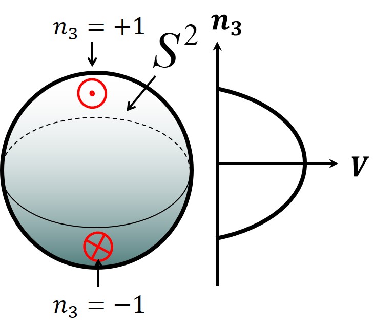
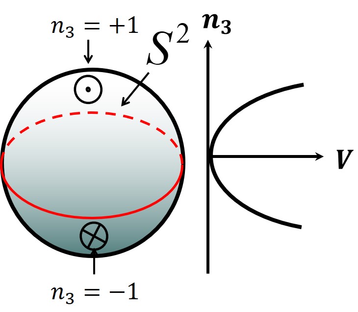
(a)	(b)

Figure 1: The potentials with vacua denoted in red. (a) Easy-axis potential. Vacua are the north ($n_{3}=+1$) and south ($n_{3}=-1$) poles. (b) Easy-plane potential. Vacua are on the equator ($n_{3}=0$).

As we show in a later section, the ground state is not a uniform state but is inhomogeneous, or forms a CSL, when the following inequality holds:

$$4\left|\kappa^{2}-2m^{2}\right|<\kappa^{2}\pi^{2}.$$ (2.30)

Then, there are a ferromagnetic phase with the easy-axis potential, the CSL phases with the easy-axis or easy-plane potential, and a helimagnetic phase at the boundary between the latter. In summary, by gradually increasing the DM interaction $\kappa$, there are the following phases:

$$\left\{\begin{array}[]{ccl}\kappa^{2}=0&:&{\rm SUSY}\\ 0\leq\kappa^{2}\leq\displaystyle{\frac{8m^{2}}{\pi^{2}+4}}&:&{\rm Ferromagnetic}\\ \displaystyle{\frac{8m^{2}}{\pi^{2}+4}}\leq\kappa^{2}<2m^{2}&:&\mbox{Easy-axis CSL}\\ \kappa^{2}=2m^{2}&:&\mbox{Helimagnetic}\\ 2m^{2}<\kappa^{2}&:&\mbox{Easy-plane CSL}\end{array}\right..$$ (2.36)

The phase diagram is given in Fig. 2.

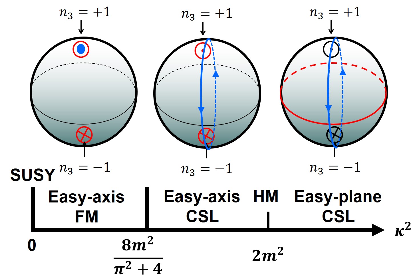
Figure 2: The Phase diagram of the chiral magnet from D-branes. FM and HM denote ferromagnetic and helimagnetic, respectively. In the FM phase, the ground state denoted by a blue dot is either the north pole $n_{3}=+1$ or south pole $n_{3}=-1$. In the easy-axis (plane) CSL, while the vacua are the north and south poles (equator), the ground state is a CSL represented by a blue circle.

3 Chiral Magnets from D-branes

In this section, we introduce two D-brane configurations in type-IIA/B string theory. In Sec. 3.1, we give the Hanany-Witten brane configuration consisting of D3, D6, NS5-branes in type-IIB string theory. In Sec. 3.2, we give fractional D2-D6 branes on the Eguchi-Hanson manifold In both cases, the $O(3)$ nonlinear sigma model is realized on the color D-brane, and we further introduce non-Abelian magnetic fluxes on the flavor D-branes inducing the DM interaction.

3.1 Hanany-Witten D-brane configuration

As mentioned, the gauge theory introduced in the last section can be made ${\cal N}=2$ SUSY by introducing the Higgs scalar fields $\tilde{\Phi}$ and adding fermionic superpartners (Higgsinos) for hypermultiplets, and gauginos for gauge or vector multiplets Eto:2006pg . Then, the theory can be realized by D-brane configurations. We first consider the Hanany-Witten brane configuration in type IIB string theory Hanany:1996ie ; Giveon:1998sr . Here, we construct a more general Grassmann sigma model with the target space

$$Gr_{N_{\rm F},N_{\rm C}}=\frac{SU(N_{\rm F})}{SU(N_{\rm C})\times SU(N_{\rm F}-N_{\rm C})\times U(1)}$$ (3.1)

by considering the ${\cal N}=2$ SUSY $U(N_{\rm C})$ gauge theory coupled with $N_{\rm F}$ hypermultiplets in the fundamental representation, and later restrict ourselves to $N_{\rm F}=2$ and $N_{\rm C}=1$ for the ${\mathbb{C}}P^{1}$ model.

In Table 1, we summarize the directions in which the D-branes extend, and the brane configuration is schematically drawn in Fig. 3.

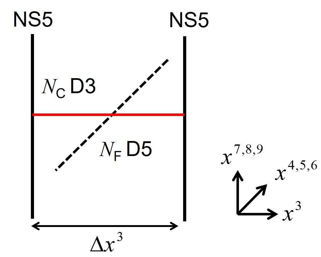
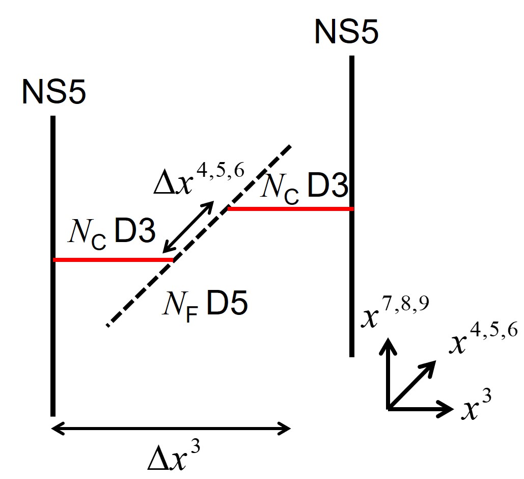
a)	b)
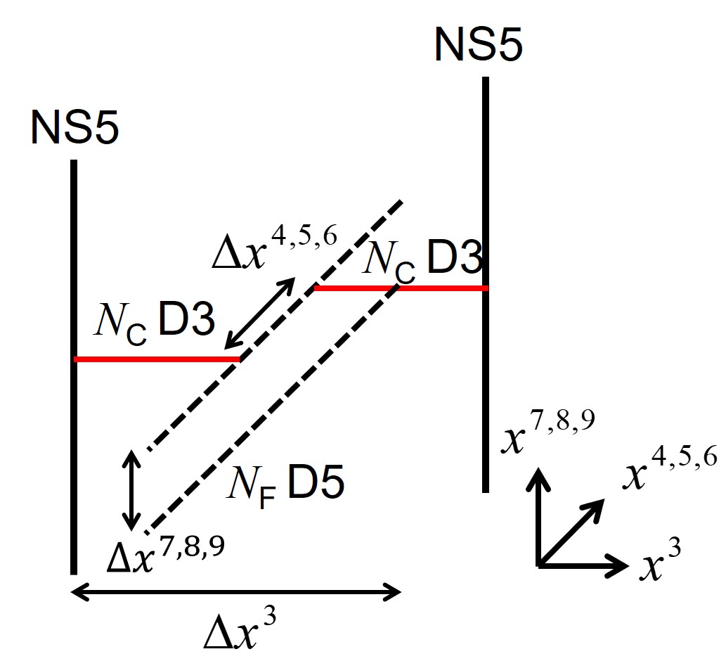
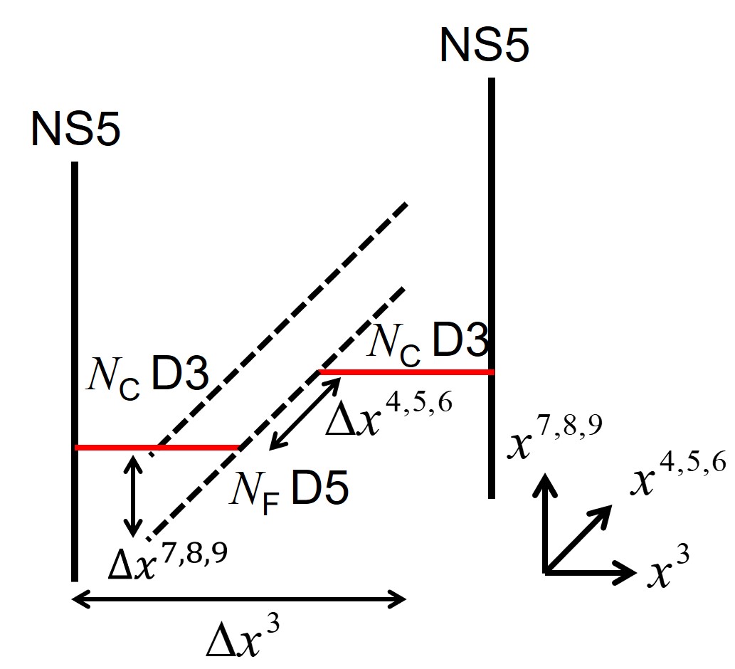
c)	d)

Figure 3: The Hanany-Witten brane configuration. The $U(N_{\rm C})$ gauge theory is realized on the worldvolume of the $N_{\rm C}$ D3-branes. Strings connecting two D3-branes give gauge multiplets while string connecting a D3-brane and a D6-brane give hypermultiplets. The separation $\Delta x^{3}$ of the two NS5-branes into the $x^{3}$ direction corresponds to $1/g^{2}$. a) Hypermultiplets are massless, and do not have a VEV. b) A triplet of FI-terms is introduced by separation $(\Delta x^{4},\Delta x^{5},\Delta x^{6})$ of the two NS5-branes into the $x^{4,5,6}$ directions. c) and d) The masses of the hypermultiplets are introduced by the separation of D5-branes into the $x^{7,8,9}$ directions.

	$x^{0}$	$x^{1}$	$x^{2}$	$x^{3}$	$x^{4}$	$x^{5}$	$x^{6}$	$x^{7}$	$x^{8}$	$x^{9}$
$N_{\rm C}$ $\rm D3$	$\circ$	$\circ$	$\circ$	$\circ$	$-$	$-$	$-$	$-$	$-$	$-$
$N_{\rm F}$ $\rm D5$	$\circ$	$\circ*$	$\circ*$	$-$	$\circ$	$\circ$	$\circ$	$-$	$-$	$-$
$2\;{\rm NS}5$	$\circ$	$\circ$	$\circ$	$-$	$-$	$-$	$-$	$\circ$	$\circ$	$\circ$

Table 1: The Hanany-Witten brane configuration. Branes are extended along directions denoted by $\circ$, and are not extended along directions denoted by $-$. $*$ denotes a background gauge field strength making D5-branes magnetized.

In Fig. 3 a), $N_{\rm C}$ D3-branes are stretched between two ${\rm NS}5$ branes separated into the $x^{3}$ direction. The $U(N_{\rm C})$ gauge theory is realized on the $N_{\rm C}$ coincident D3-brane world-volume. The $\rm D3$-brane world-volume have the finite length $\Delta x^{3}$ between two ${\rm NS}5$-branes, and therefore the $\rm D3$-brane world-volume theory is $(2+1)$-dimensional $U(N_{\rm C})$ gauge theory.

The positions of the $N_{\rm F}$ $\rm D5$ branes in the $x^{7}$-, $x^{8}$- and $x^{9}$-directions coincide with those of the $\rm D3$ branes. Strings which connect between D3 and D5 branes give rise to the $N_{\rm F}$ hypermultiplets (the Higgs fields $\Phi,\tilde{\Phi}$ and Higgsinos) in the D3-brane worldvolume theory.

Next, we put the system into the Higgs phase by separating the positions of the two NS5-branes in the $x^{4,5,6}$ directions, $(\Delta x^{4},\Delta x^{5},\Delta x^{6})\neq 0$, as in Fig. 3 b). This gives rise to the triplet of the Fayet-Iliopoulos(FI) parameters $c^{a}$ Hanany:2003hp ; Hanany:2004ea , and we choose it as $c^{a}=(0,0,v^{2}=\Delta x^{4}/g_{s}l_{s}^{2}>0)$. Then, the D3-brane worldvolue is cut and each segment of a D3-brane ends on one D5-brane.

In the third step, we introduce masses to the hypermultiplets, by separating the positions of the D5-branes into the $x^{7,8,9}$ directions as in Fig. 3 c) and d). This gives rise to triplet masses to the hypermultiplets. We consider real masses with $\Delta x^{7}=0$ for simplicity.

The vacua of the D3-brane worldvolume theory can be considered as follows. As shown in Fig. 3 c) and d), each $\rm D3$ brane ends on one of the $\rm D5$ branes, on each of which at most one $\rm D3$ brane can end, which is known as the s-rule Hanany:1996ie . There are ${}_{N_{\rm F}}C_{N_{\rm C}}=N_{\rm F}!/N_{\rm C}!(N_{\rm F}-N_{\rm C})!$ vacua in the Grassmann sigma model Arai:2003tc . The case of $N_{\rm F}=2,N_{\rm C}=1$ that we concern in this paper, there are two vacua as in Fig. 3 c) and d), corresponding to the antipodal points on ${\mathbb{C}}P^{1}\simeq S^{2}$.

Finally, we turn on a background gauge field in Eq. (2.14), Eq. (2.15) or (2.20), on the $x^{1}$-$x^{2}$ plane in the D5-brane worldvolume, which are the common directions with D3-brane worldvolume not shown in Fig. 3. Such a background gauge field makes D5-branes magnetized Bachas:1995ik ; Berkooz:1996km ; Blumenhagen:2000wh ; Angelantonj:2000hi ; Cremades:2004wa ; Kikuchi:2023awm ; Abe:2021uxb , and the $SU(N_{\rm F}=2)$ symmetry, which is a gauge symmetry on the D5-banes, is spontaneously broken to the $U(1)$ subgroup generated by $\sigma_{3}$. This background gauge field induces the DM term on the D3 brane worldvolume theory, as in the second term in Eq. (2.12), or more explicitly Eq. (2.22) or (2.24). SUSY is completely broken at this step. We will see that this final step gives very nontrivial physics. In particular, we will find that the ground states are not uniform anymore in general as summarized in Fig. 2. Before discussing that, we give another useful brane configuration related to this brane configuration.

3.2 D2-D6 system on Eguchi-Hanson space

We take a T-duality in the $x^{3}$ direction along which the NS5-branes are separated to obtain a D$2$-D$6$ system with $N_{\rm C}$ D$2$-branes and $N_{\rm F}$ D$6$-branes in type-IIA string theory Eto:2004vy , see Table 2.

	$x^{0}$	$x^{1}$	$x^{2}$	$x^{3}$	$x^{4}$	$x^{5}$	$x^{6}$	$x^{7}$	$x^{8}$	$x^{9}$
$N_{\rm C}$ $\rm D2$	$\circ$	$\circ$	$\circ$	$-$	$-$	$-$	$-$	$-$	$-$	$-$
$N_{\rm F}$ $\rm D6$	$\circ$	$\circ*$	$\circ*$	$\circ$	$\circ$	$\circ$	$\circ$	$-$	$-$	$-$
ALE ${\mathbb{C}}^{2}/{\mathbb{Z}}_{2}$	$-$	$-$	$-$	$\circ$	$\circ$	$\circ$	$\circ$	$-$	$-$	$-$

Table 2: D2-D6-brane configuration on the Eguchi-Hanson manifold in type-IIA string theory. Branes are extended along directions denoted by $\circ$, and are not extended along directions denoted by $-$.

The hypermultiplets come from strings stretched between D$2$- and D$6$-branes. First, we consider the case that all hypermultiplets are massless. In this duality, NS5-branes are mapped to a hyper-Kähler geometry. The orthogonal space ${\mathbb{C}}^{2}$ (the $x^{3,4,5,6}$ directions) perpendicular to the D$2$-branes inside the D$6$-brane world-volume is divided by ${\mathbb{Z}}_{2}$, and there is a constant self-dual NS-NS $B$-field on ${\mathbb{C}}^{2}/{\mathbb{Z}}_{2}$. The asymptotically locally Euclidean space (ALE) space of the $A_{1}$-type, the Eguchi-Hanson space $T^{*}{\mathbb{C}}P^{1}$, is obtained by blowing up the orbifold singularity by inserting $S^{2}$. The D$2$-branes are actually fractional D$2$-branes, that is, D$4$-branes two of whose spatial directions in the whole 4+1 dimensional world-volumes are wrapped around $S^{2}$, which blows up the orbifold singularity of ${\mathbb{C}}^{2}/{\mathbb{Z}}_{2}$. Thus, the positions of fractional D$2$-branes inside the D$6$-branes are fixed at the fixed point of the ${\mathbb{Z}}_{2}$ action, and thus there are no adjoint hypermultiplets on the D$2$-brane world-volume theory, see Fig. 4 a).

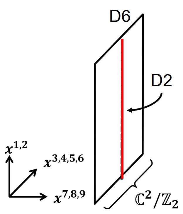
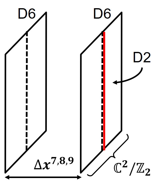
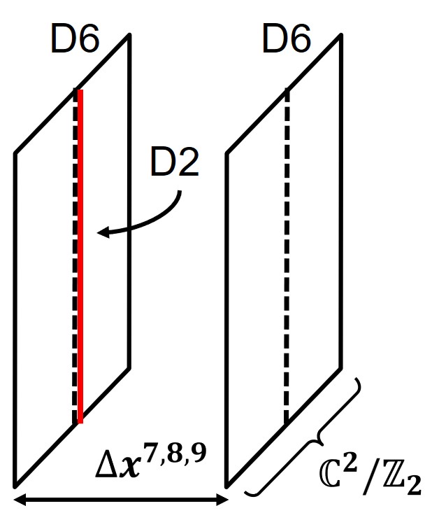
a)	b)	c)

Figure 4: The D2-D6 branes in the Eguchi-Hanson manifold in type-IIA string theory. The case of $N_{\rm F}=2$ and $N_{\rm C}=1$ is drawn. The dashed lines denote the fixed points (orbifold singularity) of the ${\mathbb{Z}}_{2}$ action on the orbifold ${\mathbb{C}}^{2}/{\mathbb{Z}}_{2}$. The singularity is blown up by $S^{2}$ to become the Eguchi-Hanson manifold. The D2-branes are fractional D2-branes, that is D4-branes two of whose worldvolume wrap $S^{2}$. a) The D-brane configuration for massless hypermultiplets in the fundamental representation. b) The brane configuration for massive hypermultiplets. Hypermultiplets coming from strings stretched between D$2$- and D$6$-branes become massive by placing D$6$-branes with distances in the $x^{7,8,9}$-coordinates.

The $N_{\rm C}$ D$2$-branes can be interpreted as Yang-Mills instantons (with the instanton number $N_{\rm C}$) on the Eguchi-Hanson manifold in the effective $U(N_{\rm F})$ gauge theory on the D$6$-branes. The Kronheimer-Nakajima construction Kronheimer1990 of the moduli space of instantons in the ALE space gives the same moduli space of vacua $T^{*}Gr_{N_{\rm F},N_{\rm C}}$ as that of the Hanany-Witten brane configuration.

Now we turn on the masses of the hypermultiplets. The masses of the hypermultiplets correspond to the positions of the D$6$-branes in the $x^{7,8,9}$-directions. Thus, the hypermultiplets coming from strings stretched between D$2$- and D$6$-branes become massive by this separation. We assume real masses for hypermultiplets by placing D6-branes parallel along the $x^{7}$-direction. To be consistent with the s-rule in the T-dual picture at most one D2-brane can be absorbed into the ${\mathbb{Z}}_{2}$ fixed point of one D6-brane.

Again, we finally turn on a background gauge field (2.14) making D6-branes magnetized. This yields the DM term, given in Eq. (2.15) or (2.20), on the D2-brane worldvolume theory.

In the following sections, we discuss brane configurations corresponding to topological solitons and modulated ground states. For such purpose, we will see that the latter brane configuration is simpler.

4 Domain Walls and Chiral Soliton Lattice Phases as D-branes

In this section, we analytically consider topological solitons of codimension one and the ground states which are also codimension one (or uniform). In Subsec. 4.1, we reduce the model to the so-called chiral sine-Gordon model by assuming one dimensional dependence. In Subsec. 4.2, we construct a magnetic domain wall as an excited state in the ferromagnetic phase and a kinky D-brane configuration. In Subsec. 4.3, we construct the CSL phase with the easy-axis potential and snaky D-brane configuration. In Subsec. 4.4, we study the helimagnetic phase. In Subsec. 4.5. we construct the CSL phase with the easy-plane potential and zigzag D-brane configuration.

4.1 Chiral sine-Gordon model

First, we introduce rotated coordinates $(\tilde{x}^{1},\tilde{x}^{2})$ by

$$\left\{\begin{array}[]{l}\tilde{x}^{1}=\cos\beta x^{1}+\sin\beta x^{2}\\ \tilde{x}^{2}=-\sin\beta x^{1}+\cos\beta x^{2}\end{array}\right..$$ (4.1)

In the next subsection, we will take $\tilde{x}^{1}$ as the direction perpendicular to the domain wall, $\tilde{x}^{2}$ the direction along the domain-wall worldvolume. Writing $\frac{\partial}{\partial\tilde{x}^{k}}=\tilde{\partial}_{k}$, we have

$${\cal H}_{\rm DM}=\bm{A}_{k}\cdot\left({\bf n}\times\partial_{k}{\bf n}\right)=\tilde{\bm{A}}_{k}\cdot\left({\bf n}\times\tilde{\partial}_{k}{\bf n}\right)$$ (4.2)

where

$$\begin{split}&\tilde{\bm{A}}_{1}=-\kappa(\cos\tilde{\vartheta},-\sin\tilde{\vartheta},0)\\ &\tilde{\bm{A}}_{2}=-\kappa(\sin\tilde{\vartheta},\cos\tilde{\vartheta},0)\end{split}$$ (4.3)

with $\tilde{\vartheta}\equiv\vartheta-\beta$.

We employ the ansatz for configurations depending on only one direction that we take $\tilde{x}^{1}$ (domain walls and chiral soliton lattices) of the form

$${\bf n}=\left(\cos\phi\sin f(\tilde{x}^{1}),\sin\phi\sin f(\tilde{x}^{1}),\cos f(\tilde{x}^{1})\right).$$ (4.4)

Then, the DM interaction can be written as

$${\cal H}_{\rm DM}=\tilde{\bm{A}}_{k}\cdot\left({\bf n}\times\tilde{\partial}_{k}{\bf n}\right)=\tilde{\bm{A}}_{1}\cdot\left({\bf n}\times\tilde{\partial}_{1}{\bf n}\right)=\kappa\sin(\tilde{\vartheta}+\phi)\tilde{\partial}_{1}f$$ (4.5)

So, one gets the chiral sine-Gordon model

$${\cal H}_{\text{SG}}=\frac{1}{2}\left(\tilde{\partial}_{1}f\right)^{2}+\kappa\sin(\tilde{\vartheta}+\phi)\tilde{\partial}_{1}f+\left(\frac{\kappa^{2}}{2}-m^{2}\right)\cos^{2}f+\frac{\kappa^{2}}{2}+m^{2}.$$ (4.6)

The second term is a total derivative term specific for the chiral sine-Gordon model, or a topological term counting the number of sine-Gordon solitons. Note that this term does not contribute to the equation of motion.

The trivial vacuum solutions are given by

$$f_{\text{vac}}=\left\{\begin{array}[]{clll}\left(l+\frac{1}{2}\right)\pi&~{}~{}\text{if}&\kappa^{2}-2m^{2}>0&~{}\text{(easy-plane)}\\ l\pi&~{}~{}\text{if}&\kappa^{2}-2m^{2}<0&~{}\text{(easy-axis)}\end{array}\right.$$ (4.7)

with an integer $l$. When the potential term vanishes, i.e., $\kappa^{2}-2m^{2}=0$, any constant can be the vacuum solution.

The chiral sine-Gordon model or chiral double sine-Gordon model also appears in QCD at finite density in the presence of strong magnetic field Son:2007ny ; Brauner:2016pko or rapid rotation Nishimura:2020odq ; Eto:2021gyy . In such cases, the Wess-Zumino-Witten term Son:2004tq gives a topological term instead of the DM term.

4.2 Domain walls in ferromagnetic phase with easy-axis potential

First, we consider the ferromagnetic phase. In this phase, there are two vacua corresponding to the north and south poles $n_{3}=\pm 1$. In terms of the D-brane configurations, they correspond to the straight D-branes in Fig. 3 c) and d) for the Hanany-Witten brane configuration in type-IIB string theory and Fig. 4 b) and c) for the D2-D6-ALE system in type-IIA string theory.

Then, we consider a magnetic domain wall interpolating these two vacua. In this case, the energy per unit length in the $\tilde{x}^{2}$-direction is given by

$$E[f] \equiv\int d\tilde{x}^{1}{\cal H}_{\text{SG}}$$

$$=\int d\tilde{x}^{1}\left[\frac{1}{2}\left(\tilde{\partial}_{1}f\right)^{2}+\kappa\sin(\tilde{\vartheta}+\phi)\tilde{\partial}_{1}f+\left(m^{2}-\frac{\kappa^{2}}{2}\right)\sin^{2}f\right]+E_{\text{vac}}^{\text{e.a.}}\ ,$$ (4.8)

where $E_{\text{vac}}^{\text{e.a.}}$ denotes the vacuum energy with the easy-axis potential. Let us study a single kink solution. The (anti-)BPS equation for the magnetic domain wall can be given by

$$\tilde{\partial}_{1}f=\pm\sqrt{2m^{2}-\kappa^{2}}\sin f.$$ (4.9)

The solution can be obtained as

$$f_{\text{kink}}=2\arctan\left[\exp\left(\pm\sqrt{2m^{2}-\kappa^{2}}\tilde{x}^{1}+X\right)\right]\ ,$$ (4.10)

where $X$ is a position moduli parameter. If we choose the plus (minus) sign for the (anti-)BPS soliton, the function $f$ monotonically increases (decreases). The equation for the phase $\phi$ is simply given by

$$\cos(\tilde{\vartheta}+\phi)=0\ .$$ (4.11)

For the lowest energy kink solutions, the second term in the energy (4.8), which stems from the DM interaction, should be negative, so that $\phi$ is chosen as

$$\phi=\left\{\begin{matrix}-\tilde{\vartheta}-\frac{\pi}{2}&&\text{if~{}~{}}\kappa~{}\tilde{{\partial}}_{1}f>0\ ,\\ -\tilde{\vartheta}+\frac{\pi}{2}&&\text{if~{}~{}}\kappa~{}\tilde{{\partial}}_{1}f<0\ .\end{matrix}\right.$$ (4.12)

For the phase $\phi$ giving the lowest energy kink solution, one finds that the energy difference between the single kink solution and the vacuum state is given by

$$E\left[f_{\text{kink }}\right]-E_{\text{vac}}^{\text{e.a.}}=2\sqrt{2m^{2}-\kappa^{2}}-|\kappa|\pi\ .$$ (4.13)

See Fig. 5 a) for a plot of the single domain wall (4.10). One of the most important role of the presence of the DM term is that this domain wall does not carry a $U(1)$ modulus Ross:2022vsa ; the $U(1)$ phase $\phi$ is fixed to be a constant determined from $\vartheta$ through Eq. (4.11). When $\bf n$ at the domain wall ($n_{3}=0$) is parallel or orthogonal to the domain wall worldvolume, the wall is called Bloch or Néel, respectively, see Table 3.

Type	$\tilde{\vartheta}$	$\phi$	$S^{1}$	to DW
Bloch	$0$	$\pm\pi/2$	$n_{1}=0$	parallel
Néel	$\pm\pi/2$	$\pm\pi$	$n_{2}=0$	orthogonal

Table 3: Bloch or Néel type magnetic domain wall. The parameter $\tilde{\vartheta}$, $U(1)$ phase $\phi$ of the domain wall, $S^{1}$ submanifold inside target space $S^{2}$, and relation of ${\bf n}$ to the domain wall worldvolume.

We can change the direction of the domain wall worldvolume by changing $\beta$ in Eq. (4.1) with the same ansatz in Eq. (4.4). Then, the $U(1)$ phase $\phi$ changes accordingly through Eq. (4.11), and the angle between the $U(1)$ phase $\phi$ and the spatial direction of the domain wall worldvolume is preserved under a rotation. This is well known and was reconfirmed in the effective theory of the domain wall Ross:2022vsa .

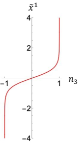
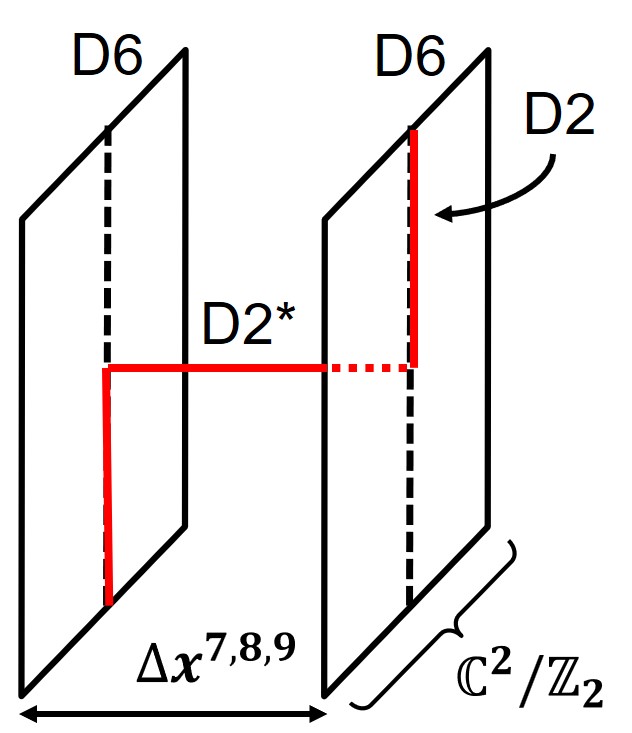
(a)	(b)

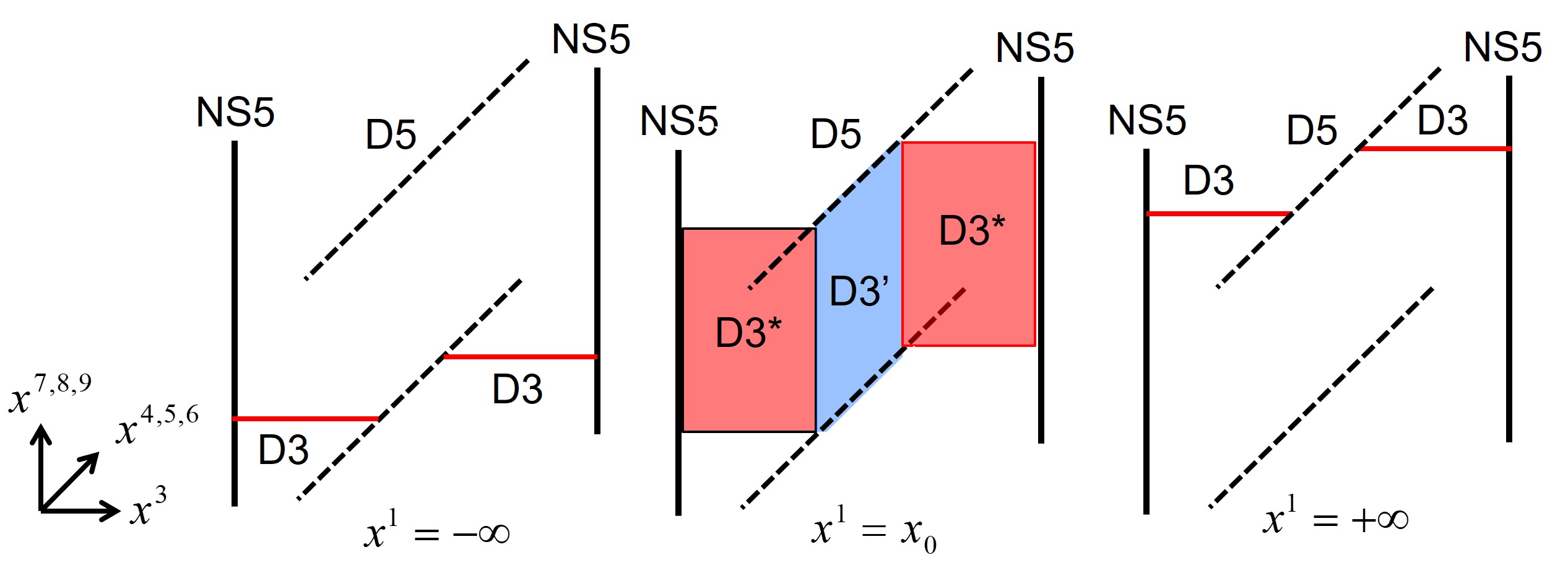
(c)

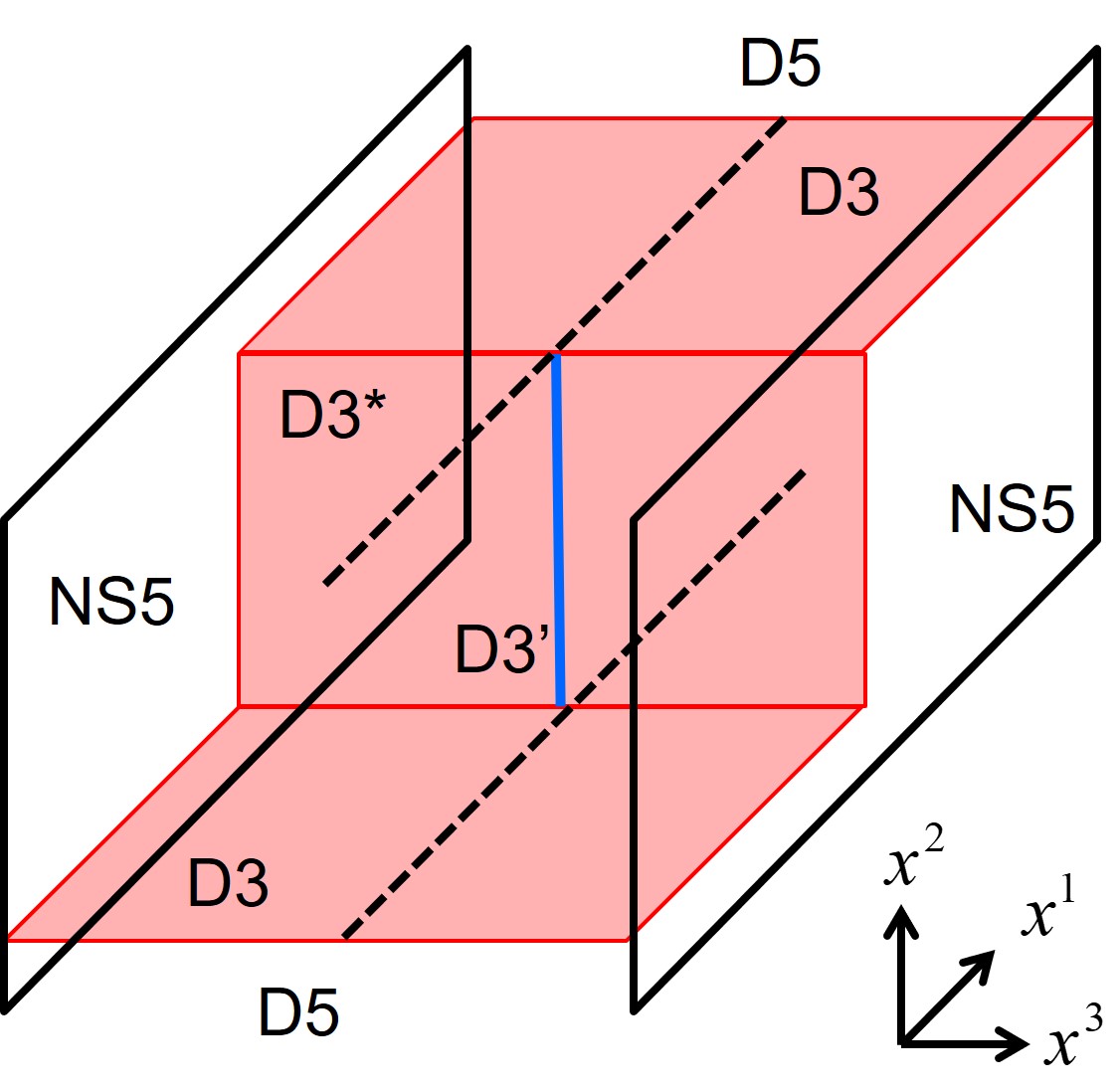
(d)

Figure 5: (a) A single magnetic domain wall with the easy potential at the critical point ($\kappa=1,m^{2}=(\pi^{2}-4)/8$). The corresponding kinky brane configuration in (b) the D2-D5-ALE system and (c), (d) the Hanany-Witten brane configuration.

Now let us discuss D-brane configurations for the magnetic domain wall. In the D2-D6-ALE system in type-IIA string theory, the effective theory on the D$2$-brane is the SUSY $U(N_{\rm C})$ gauge theory with massive $N_{\rm F}$ hypermultiplets and the FI-term. For $N_{\rm C}=1,N_{\rm F}=2$ that we are considering, $\Sigma=mn_{3}$ for a single magnetic domain-wall solution is plotted as a function of $x^{1}$: $x^{7}=\Sigma(x^{1})$ in Fig. 5 (b) left. It represents a kinky D$2$-brane curved in the ($x^{1}$,$x^{7}$)-plane and the curve is determined by the solution (4.10) Lambert:1999ix ; Eto:2004vy ; Eto:2006mz ; Eto:2007aw ; Misumi:2014bsa . In the limit of a thin domain wall Hanany:2005bq , the part of the kinky D2-brane can be regarded as a D2-brane extending into the $x^{7}$-direction instead of the $x^{1}$ direction (the codimension of the wall). We denote it by D2^∗ (see Fig. 5(b) right) and the brane configuration is summarized in Table 4.

	$x^{0}$	$x^{1}$	$x^{2}$	$x^{3}$	$x^{4}$	$x^{5}$	$x^{6}$	$x^{7}$	$x^{8}$	$x^{9}$
$N_{\rm C}$ $\rm D2$	$\circ$	$\circ$	$\circ$	$-$	$-$	$-$	$-$	$-$	$-$	$-$
$\rm D2^{*}$	$\circ$	$-$	$\circ$	$-$	$-$	$-$	$-$	$\circ$	$-$	$-$
$N_{\rm F}$ $\rm D6$	$\circ$	$\circ*$	$\circ*$	$\circ$	$\circ$	$\circ$	$\circ$	$-$	$-$	$-$
ALE ${\mathbb{C}}^{2}/{\mathbb{Z}}_{2}$	$-$	$-$	$-$	$\circ$	$\circ$	$\circ$	$\circ$	$-$	$-$	$-$

Table 4: The domain wall in the D2-D6-brane configuration on the Eguchi-Hanson manifold in type-IIA string theory. Branes are extended along directions denoted by $\circ$, and are not extended along directions denoted by $-$.

Next, let us discuss a magnetic domain wall in the Hanany-Witten configuration in type-IIB string theory Eto:2004vy . In this case, the position of the D3-brane at the $x^{7}$-coordinate depends on the $x^{1}$ coordinate for a magnetic domain wall. Around the domain wall at $x^{1}=x_{0}$, they move from one D5-brane to the other D5-brane. Here, we consider the thin-wall limit for simplicity. In Fig. 5 (c), they are represented by D3^∗. However, they can end on no D5 brane and must be bent to the $x^{4}$-direction to join to each other by creating a segment represented by D3^′. In Fig. 5 (d), the same configuration is shown with plotting the $x^{1}$ direction and suppressing the $x^{4}$ direction. The brane configuration is summarized in Table 5 .

	$x^{0}$	$x^{1}$	$x^{2}$	$x^{3}$	$x^{4}$	$x^{5}$	$x^{6}$	$x^{7}$	$x^{8}$	$x^{9}$
$N_{\rm C}$ $\rm D3$	$\circ$	$\circ$	$\circ$	$\circ$	$-$	$-$	$-$	$-$	$-$	$-$
D3′	$\circ$	$-$	$\circ$	$-$	$\circ$	$-$	$-$	$\circ$	$-$	$-$
D3∗	$\circ$	$-$	$\circ$	$\circ$	$-$	$-$	$-$	$\circ$	$-$	$-$
$N_{\rm F}$ $\rm D5$	$\circ$	$\circ*$	$\circ*$	$-$	$\circ$	$\circ$	$\circ$	$-$	$-$	$-$
$2\;{\rm NS}5$	$\circ$	$\circ$	$\circ$	$-$	$-$	$-$	$-$	$\circ$	$\circ$	$\circ$

Table 5: The domain wall in the Hanany-Witten brane configuration: Branes are extended along directions denoted by $\circ$, and are not extended along directions denoted by $-$.

4.3 Chiral soliton lattice phase with easy-axis potential

We now discuss inhomogeneous ground states. Here, we give the condition that the CSL is the ground state instead of uniform configurations. As implied by the energy difference between the single soliton and the vacuum (uniform) configuration (4.13), the kink energy can be lower than the vacuum energy. In such a case, solitons are created in the vacuum, and eventually they form a CSL, an array of kinks and anti-kinks. Thus, a CSL is the ground state if

$$4\left(2m^{2}-\kappa^{2}\right)<\kappa^{2}\pi^{2}.$$ (4.14)

The CSL solutions are given in terms of the Jacobi amplitude function as

$$f_{\text{CSL}}=\pm\mathrm{am}\left(\frac{\sqrt{2m^{2}-\kappa^{2}}}{\lambda}\tilde{x}^{1}+X,\lambda\right)+\frac{\pi}{2}\ .$$ (4.15)

It would be worth noting that Eq. (4.15) solves the Euler-Lagrange equation obtained from the energy functional for any $\lambda\in(0,1]$, but does not satisfy the BPS equation (4.9), except for the case $\lambda=1$ where it reduces to the single-kink solution (4.10). The solution (4.15) with the plus (minus) sign is a monotonically increasing (decreasing) function of $\tilde{x}^{1}$. To obtain the ground state, the phase $\phi$ should be taken as Eq. (4.12). In addition, the modulus $\lambda$ for the ground state is determined through

$$2\mathrm{E}(\lambda)=\frac{|\kappa|\pi}{\sqrt{2m^{2}-\kappa^{2}}}\lambda$$ (4.16)

with the elliptic integral of the second kind $\mathrm{E}(\lambda)$, which can be derived from $dE[f_{\text{CSL}}]/d\lambda=0$. Fig. 6 shows a CSL ground state for the easy-plane potential. The figure a) is a plot of the CSL solution, and b) is a schematic plot for a shape of the D2-brane in the D2-D6-ALE system, which may be called a snaky D-brane.

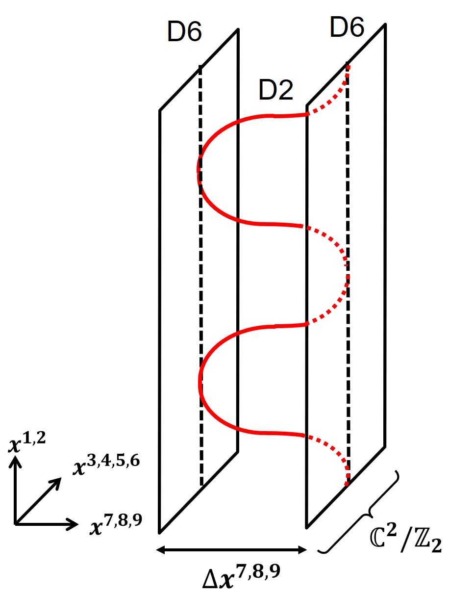
a)	b)

Figure 6: a) A CSL solution with the easy-plane potential as the ground state ($\kappa=1.0,m=1.3$). b) A snaky D2-brane corresponding to a).

4.4 Helimagnetic phase

When the relation $2m^{2}=\kappa^{2}$ holds, the total potential term vanishes, as can be seen in Eq. (2.29), and the energy per unit length can be written as

$$E[f]=\frac{1}{2}\int d\tilde{x}^{1}\left[\left\{\tilde{\partial}_{1}f+\kappa\sin\left(\tilde{\vartheta}+\phi\right)\right\}^{2}-\kappa^{2}\sin^{2}\left(\tilde{\vartheta}+\phi\right)\right]+\text{const.}$$ (4.17)

In this case, domain walls do not exist. However, the ground state is uniformly modulated due to the DM interaction. Since the BPS equation is given by

$$\tilde{\partial}_{1}f=-\kappa\sin\left(\tilde{\vartheta}+\phi\right)\ ,$$ (4.18)

the solution for the ground state is

$$\left\{\begin{array}[]{l}f=\pm\kappa\tilde{x}^{1}\\ \phi=-\tilde{\vartheta}\mp\frac{\pi}{2}\end{array}\right.\ .$$ (4.19)

Thus, in this case, the phase varies linearly.

4.5 Chiral soliton lattice phase with easy-plane potential

Next, we consider the case of the easy-plane potential. A domain wall with the easy-plane potential is not topologically stable in the sense that both of the boundaries are connected and degenerated. Such an unstable domain wall should decay into a vacuum state when the DM interaction is absent. However, in the presence of the DM interaction, such domain walls can be energetically stable. Indeed, in our setting, the ground state is always given by a CSL composed of such unstable domain walls and anti-domain walls.

For the easy-plane case, the energy per unit length in the $\tilde{x}^{2}$-direction can be defined as

$$E[f] =\int d\tilde{x}^{1}\left[\frac{1}{2}\left(\tilde{\partial}_{1}f\right)^{2}+\kappa\sin(\tilde{\vartheta}+\phi)\tilde{\partial}_{1}f+\left(\frac{\kappa^{2}}{2}-m^{2}\right)\cos^{2}f\right]+E_{\text{vac}}^{\text{e.p.}}\ ,$$ (4.20)

where $E_{\text{vac}}^{\text{e.p.}}$ denotes the vacuum energy with the easy-plane potential. Let us begin with studying a single kink solution. The (anti-)BPS equation for a single kink is given by

$$\tilde{\partial}_{1}f=\pm\sqrt{\kappa^{2}-2m^{2}}\cos f$$ (4.21)

This equation can be solved by

$$f_{\text{kink}}=\pm 2\arctan\left[\tanh\left(\frac{\sqrt{\kappa^{2}-2m^{2}}}{2}\tilde{x}^{1}+X\right)\right]$$ (4.22)

where $X$ is a position moduli parameter. For the plus (minus) sign for an (anti-)BPS kink, the function (4.22) is a monotonically increasing (decreasing) function of $\tilde{x}^{1}$. Among the kink solutions, the lowest energy is attained when $\phi$ is taken as Eq. (4.12), as the same with the easy-axis case. Fig. 7 a) shows a single kink solution in the easy-plane potential.

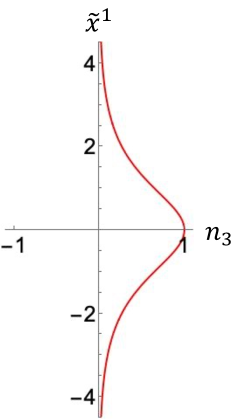
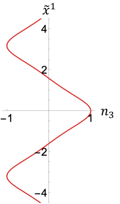
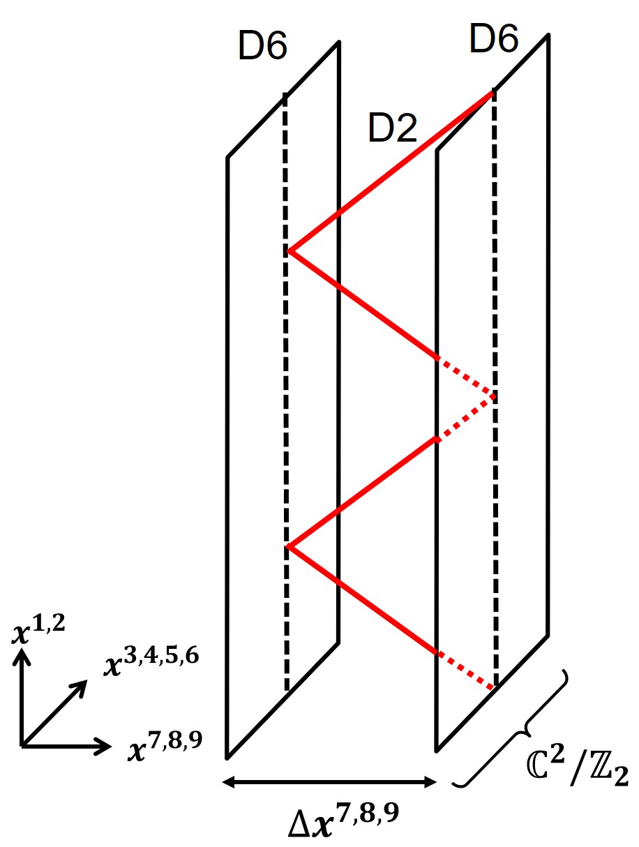
a)	b)	c)

Figure 7: a) A single domain wall and b) chiral soliton lattices with the easy-plane potential as the ground state ($\kappa=1.2,m=0.1$). c) A zigzag D2-brane corresponding to b).

As the case of the easy-axis potential, the kink can have negative energy. In such a case, the kink does not decay to the vacuum. The difference between the kink energy and vacuum energy is

$$E\left[f_{\text{kink}}\right]-E_{\text{vac}}^{\text{e.p.}}=2\sqrt{\kappa^{2}-2m^{2}}-|\kappa|\pi.$$ (4.23)

If the kink energy is less than that of uniform state (vacuum), i.e.,

$$4\left(\kappa^{2}-2m^{2}\right)<\kappa^{2}\pi^{2}$$ (4.24)

then, a CSL, an array of kinks and anti-kinks, is the ground state. Since $\pi^{2}>4$, however, this inequality always holds. Thus, for the easy-plane potential, the ferromagnetic state (vacuum) is unstable, and the CSL phase is always the ground state for any $m^{2}\in\left[0,\kappa^{2}/2\right)$.

In the case of the easy-plane potential, the solution describing a CSL is given by

$$f_{\text{CSL}}=\pm\mathrm{am}\left(\frac{\sqrt{\kappa^{2}-2m^{2}}}{\lambda}\tilde{x}^{1}+X,\lambda\right)$$ (4.25)

with a position moduli parameter $X$. Similar to the easy-axis case, the modulus $\lambda$ providing the ground state is determined through

$$2\mathrm{E}(\lambda)=\frac{|\kappa|\pi}{\sqrt{\kappa^{2}-2m^{2}}}\lambda\ .$$ (4.26)

Fig. 7 b) shows a plot of the CSL solution with the easy-plane potential, which is rather zigzag compared with that with easy-axis potential. This can be identified with a D2-brane configuration for a CSL, as schematically drawn in Fig. 7 c). The D2-brane touches the D6-branes at a shorter range than one in the easy-axis potential case shown in Fig. 6.

5 Magnetic Skyrmions as D-branes

In this section, we discuss topologically excited states of two codimensions, that is, magnetic skyrmions and domain-wall skyrmions in chiral magnets. In our model, these are excited states on top of the easy-axis ferromagnetic ground state. In Subsec. 5.1, we numerically construct magnetic skyrmions and find that they are represented by D1-branes (fractional D0-branes) in the Hanany-Witten brane configuration (D2-D6-ALE system) in type-IIB(A) string theory. In Subsec. 5.2, we numerically construct explicit solutions of domain-wall skyrmions, and see the shape to the color D-brane in the visinity of a skyrmion.

5.1 Magnetic skyrmions

In this subsection, we show that magnetic skyrmions can be described by D1-branes in the Hanany-Witten brane configuration in type-IIB string theory, or by D0-branes in the D2-D4-ALE system in type-IIB string theory. The latter are in fact fractional D0-branes, that is D2 branes two of whose spatial directions wrap around the $S^{2}$ cycle blowing up the orbifold singularity ${\mathbb{C}}^{2}/{\mathbb{Z}}_{2}$.

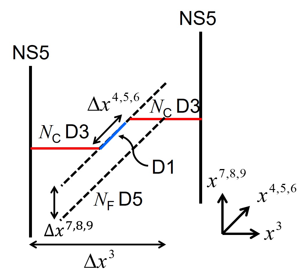
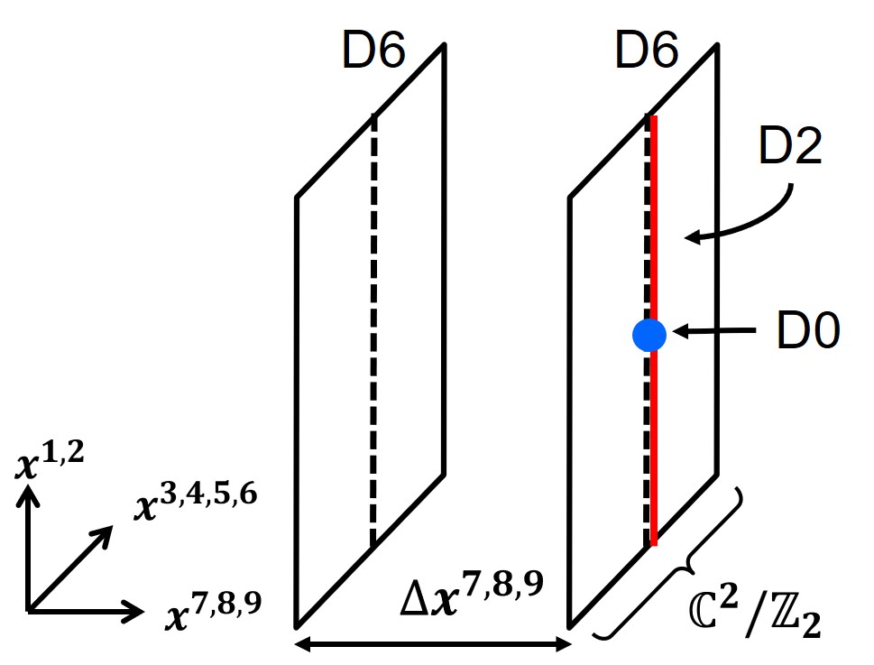
a)	b)

Figure 8: D-brane configurations for a magnetic skyrmion in a) the Hanany-Witten brane configuration and b) the D2-D6-ALE system. A magnetic skyrmion is realized by a) a D1-brane and b) a fractional D0-brane, respectively.

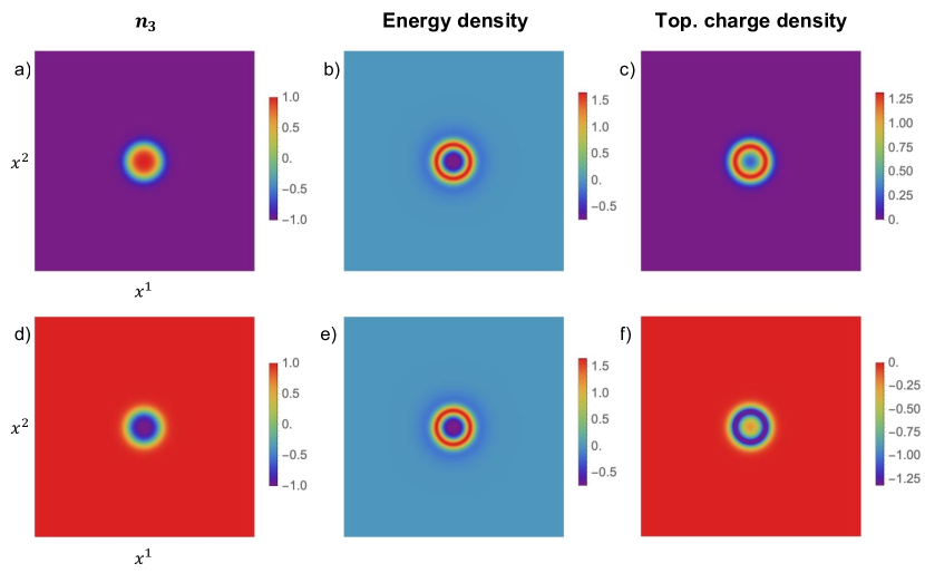
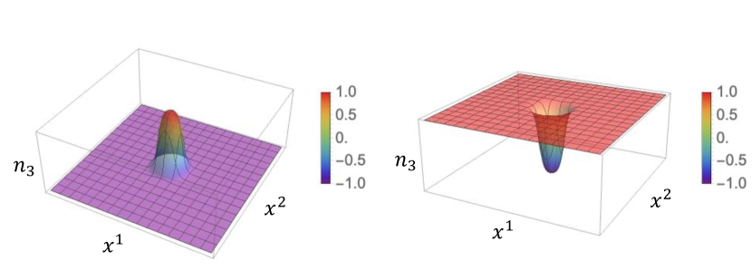
Figure 9: Skyrmion and anti-skyrmion with the easy-axis potential ($\kappa=1.0,m^{2}=2.0,\vartheta=0$). The top panels represent quantities of a skyrmion with the boundary condition $n_{3}=1$, and the bottom panels do of an anti-skyrmion with the boundary condition $n_{3}=-1$. The panels a) and d) show the value of $n_{3}$; b) and e) energy density; c) and f) topological charge density.

Figure 10: Shape of a D2-brane for a single skyrmion (left) and anti-skyrmion (right) with the easy-axis potential ($\kappa=1.0,m^{2}=2.0,\vartheta=0$)

Let us start with the case in the absence of the DM term and masses of scalar fields ($\Delta x^{7,8,9}=0$). In such a case, vortices were previously realized as D1-branes in the Hanany-Witten brane configuration, or as D0-branes in the D2-D6 system, as in Fig. 8 a) or b), respectively Hanany:2003hp . These vortices are non-Abelian vortices in general Hanany:2003hp ; Auzzi:2003fs ; Eto:2005yh ; Eto:2006cx ; Shifman:2007ce ; Shifman:2009zz ; Eto:2004rz . For $N_{\rm F}=N_{\rm C}\equiv N$ they are local non-Abelian vortices with non-Abelian orientational moduli ${\mathbb{C}}P^{N-1}$, where the case of $N=1$ corresponds to Abrikosov-Nielsen-Olesen (ANO) vortices Abrikosov:1956sx ; Nielsen:1973cs in superconductors. For $N_{\rm F}>N_{\rm C}$ such as our concern of $N_{\rm C}=1,N_{\rm F}=2$, they are semi-local vortices Vachaspati:1991dz ; Achucarro:1999it ; Shifman:2006kd ; Eto:2007yv having size and phase moduli in addition to non-Abelian orientational moduli.

In the strong gauge coupling limit, $\Delta x^{3}\sim 1/g^{2}=0$, these semi-local vortices ($N_{\rm F}>N_{\rm C}$) become lumps in a nonlinear sigma model, which still possess size and phase moduli. In the case of $N_{\rm C}=1,N_{\rm F}=2$, they are ${\mathbb{C}}P^{1}$ lumps.

If we turn on masses of scalar fields ($\Delta x^{7,8,9}\neq 0$), semilocal vortices at finite gauge coupling $g$ shrink, the size modulus becomes zero, and they eventually become ANO votices. However, in the strong gauge coupling limit, lumps are not stable in such a mass deformation; they shrink to zero size and configurations become singular (called small lump singularity).

Now we introduce the DM interaction by turning on the background gauge field (2.14) on the D5(D6)-branes in the Hanany-Witten configuration (the D2-D4-ALE system). Then, the D5(D6)-branes become so-called magnetized D-branes Bachas:1995ik ; Berkooz:1996km ; Blumenhagen:2000wh ; Angelantonj:2000hi ; Cremades:2004wa ; Kikuchi:2023awm ; Abe:2021uxb , and the $SU(2)$ gauge symmetry on the brane is spontaneously broken to $U(1)$. This induces the DM interaction on the D3(D2)-brane worldvolume field theory, where the $SU(2)$ flavor symmetry is broken to $U(1)$. The Hamiltonian density is given in Eq. (2.12), and the energy can be written as

$$E \equiv\int d^{2}x{\cal H}$$

$$=\int d^{2}x\left[\frac{1}{2}\partial_{k}{\bf n}\cdot\partial_{k}{\bf n}+\kappa\left\{\cos\vartheta~{}{\bf n}\cdot(\nabla\times{\bf n})-\sin\vartheta({\bf n}\cdot\nabla n_{3}-n_{3}\nabla\cdot{\bf n})\right\}\right.$$

$$\hskip 227.62204pt\left.+\left(m^{2}-\frac{\kappa^{2}}{2}\right)(1-n_{3}^{2})\right]+\text{const.}$$ (5.1)

where the second term is the induced DM interaction, and the third is the easy-axis potential. This induced DM interaction prevents lumps from shrinking, which are nothing but magnetic skyrmions. Indeed, the Derick’s scaling argument Ross:2022vsa requires that for stable configurations of codimension two, the energy contribution from the DM interaction energy $E_{\text{DM}}$ and the potential energy $E_{\text{pot}}$ satisfy the relation

$$E_{\text{DM}}+2E_{\text{pot}}=0\ ,$$ (5.2)

implying that non-trivial skyrmion solutions can exist only when the DM interaction energy is a finite negative value. The topological charge of the skyrmion, $\pi_{2}(S^{2})$, is defined by

$$Q=\frac{1}{8\pi}\int d^{2}x~{}\varepsilon^{jk}{\bf n}\cdot\left(\partial_{j}{\bf n}\times\partial_{k}{\bf n}\right)\ .$$ (5.3)

Even in the presence of the DM interaction, only one of either skyrmion ($Q=+1$) or anti-skyrmion ($Q=-1$) is stable depending on the vacuum: When the vacuum is $n_{3}=-1$, a skyrmion is stable and an anti-skyrmion is unstable; On the other hand, when the vacuum is $n_{3}=+1$, an anti-skyrmion is stable and a skyrmion is unstable. This can easily be seen when we consider a rotational symmetric ansatz of the form

$${\bf n}=\left(\cos(\nu\theta+\gamma)\sin f(r),\sin(\nu\theta+\gamma)\sin f(r),\cos f(r)\right)$$ (5.4)

with the polar coordinates $(r,\theta)$, where $\nu\in\mathbb{Z}$ denotes a winding number, $\gamma\in[0,2\pi)$ is a constant describing the internal orientation of the skyrmion, and $f(r)\in[0,\pi]$ is a monotonic function satisfying the boundary conditions $\{f(0)=0,f(\infty)=\pi\}$ or $\{f(0)=\pi,f(\infty)=0\}$. Then, the DM term can be written as

$$E_{\text{DM}}=-\kappa\int d^{2}x~{}\sin[(1-\nu)\theta-\vartheta-\gamma]\left(\frac{\nu\sin(2f)}{2r}+\partial_{r}f\right)\ .$$ (5.5)

It indicates that the energy contribution from the DM interaction vanishes except for $\nu=1$. If $E_{\text{DM}}=0$, no non-trivial configuration can satisfy the relation (5.2). Therefore, stable axisymmetric configurations must have the winding number $\nu=1$. In addition, by substituting the ansatz into the topological charge, one obtains

$$Q=-\frac{\nu}{2}\left[\cos f(r)\right]_{r=0}^{r=\infty}=-\frac{\nu}{2}\left[n_{3}(r)\right]_{r=0}^{r=\infty}.$$ (5.6)

Therefore, a stable configuration with $\nu=1$ possesses $Q=\pm 1$ when the vacuum is $n_{3}=\mp 1$.

The Euler-Lagrange equation of this model is given by

$$\partial_{b}^{2}n_{a}+2\kappa\left[\sin\vartheta(\partial_{a}n_{3}-\delta_{a3}\partial_{b}n_{b})+\cos\vartheta~{}\varepsilon_{abc}\partial_{b}n_{c}\right]+(2m^{2}-\kappa^{2})\delta_{a3}n_{3}+\Lambda n_{a}=0$$ (5.7)

where $\Lambda$ is a Lagrange multiplier. Note that, different from the kink and CSL cases, the DM interaction contributes not only to the energy but also to the equation of motion. We numerically solve this equation using a conjugate gradient method with the fourth-order finite difference approximation. Our simulations are performed on a grid with $201\times 201$ lattice points and a lattice spacing $\Delta=0.1$. For the initial input, we employed the rotationally invariant configuration (5.4) with $\nu=1,\gamma=0$, and a smooth monotonic function $f(r)$ satisfying the boundary condition. In Fig. 10, we give numerical solutions for a single magnetic (anti-)skyrmion with the easy-axis potential and the Bloch-type DM interaction, i.e., $\vartheta=0$. As one can see from the energy density plots, the stable (anti-)skyrmion is in a shape of a domain wall ring, inside which the energy density is negative due to the DM interaction. Fig. 10 shows that the color D2(D3)-brane worldvolume is bent and touches to the flavor D6(D5)-brane on the opposite side around the position of the D0(D1)-brane corresponding to the magnetic skyrmion in type IIA(B) string theory.

Since there is repulsion between skyrmions, multiple skyrmion states are always unstable, as the same with the magnetic skyrmions with a Zeeman interaction Shnir2018 .

5.2 Domain-wall Skyrmions

The ferromagnetic phase admits both magnetic domain walls and magnetic skyrmions. When they coexist, they feel attraction. Thus, a magnetic skyrmion should be absorbed into a domain wall. The final state is a stable composite state called a domain-wall skyrmion Nitta:2012xq ; Kobayashi:2013ju ; Ross:2022vsa . In such a situation, the magnetic skyrmion is realized as a sine-Gordon soliton in the domain-wall effective field theory which is a sine-Gordon model with a potential term induced by the DM term Ross:2022vsa .

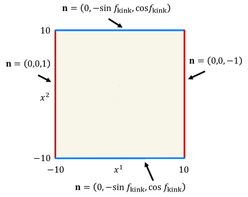
Figure 11: Boundary condition used in the numerical simulation for the domain-wall skyrmions with the parameter $\kappa>0,\vartheta=0$.

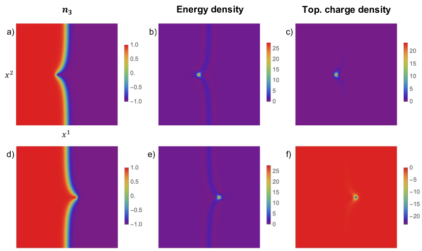
Figure 12: Domain-wall skyrmion and domain-wall anti-skyrmion with the easy-plane potential ($\kappa=1.0,m^{2}=2.0,\vartheta=0$). The top panels represent quantities of a domain-wall skyrmion, and the bottom panels do of a domain-wall anti-skyrmion. The panels a) and d) show the value of $n_{3}$; b) and e) energy density; c) and f) topological charge density. a) $n_{3}$, b) energy density, c) topological charge density.

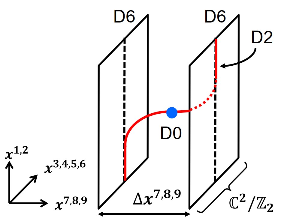
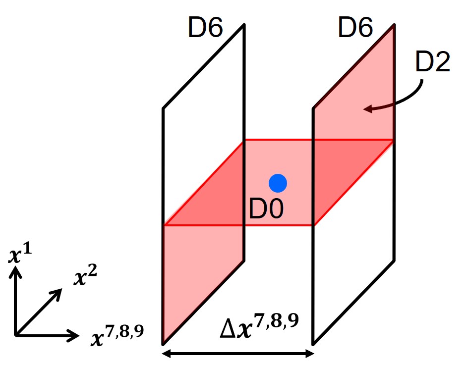
(a)	(b)

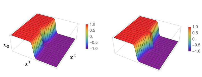
Figure 13: A kinky D2-D0-brane bound state in the D2-D6-ALE system in type-IIA string theory describing a domain-wall skyrmion. A similar configuration can be considered in the Hanany-Witten brane configuration in type-IIB string theory.

Figure 14: Shapes of the D2-brane for a domain-wall skyrmion (left) and anti-skyrmion (right) with the easy-axis potential ($\kappa=1.0,m^{2}=2.0,\vartheta=0$). The kinky shape of the D2-branes is pulled or pushed due to the D0-brane.

To obtain explicit solutions of domain-wall skyrmions, we numerically solve the equation of motion in Eq. (5.7) with the same method used in the last subsection. We run our simulations by replacing the spatial domain $[-10,10]\times[-10,10]\subset\mathbb{R}^{2}$ with a grid with $201\times 201$ lattice points and lattice spacing $\Delta=0.1$. We impose the Dirichlet boundary conditions that we assign a different vacuum to each boundary in the $x^{2}$-direction and the lowest energy single-kink solution with the easy-axis potential in Eq. (4.10) to the boundaries in the $x^{1}$-direction. In Fig. 11, we show a concrete example of the boundary condition. In the bulk, we employ the following configuration as an initial input by choosing parameters compatible with the boundary conditions:

$${\bf n}=\left(\cos\phi(x^{2})\sin f_{\text{kink}}(x^{1}),\sin\phi(x^{2})\sin f_{\text{kink}}(x^{1}),\cos f_{\text{kink}}(x^{1})\right)$$ (5.8)

where $f_{\text{kink}}$ is the single kink solution for the easy -axis case in Eq. (4.10) with the moduli parameter $X=0$, and

$$\phi=4\arctan e^{cx^{2}}-\vartheta\mp\frac{\pi}{2}$$ (5.9)

with a real parameter $c$. In Fig. 12, we present numerical solutions for domain-wall (anti-)skyrmions. The upper figures show a single skyrmion on the wall and the lower figures show a single anti-skyrmion on the wall. It is important to emphasize that both skyrmion and anti-skyrmion are stable. We can observe that the domain wall is bent in the vicinity of the (anti-)skyrmion, which is consistent with Ref. KBRBSK . The direction of the bending depends on the sign of the topological charge of the skyrmion.

In Fig. 14, we schematically draw brane configurations for a domain-wall skyrmion, as a combination of those for a domain wall and magnetic skyrmion. As a consequence of the bending of the domain wall in Fig. 12, the D2-brane worldvolume forming a kink is pulled to either direction of the wall in the vicinity of a D0-brane corresponding to the magnetic skyrmion, as shown in Fig. 14.

6 Summary and Discussion

We have given string theory construction for chiral magnets in terms of the Hanany-Witten brane configuration (consisting of D3, D5 and NS5-branes) in type-IIB string theory, and the fractional D2 and D6 branes on the Eguchi-Hanson manifold in type-IIA string theory. In both cases, the flavor branes are magnetized by a constant magnetic flux. The $O(3)$ sigma model with the DM interaction describing chiral magnets is realized on the worldvolume of the color D-branes. As summarized in Fig. 2, we have found that the ground states are not uniform in general: The ground state is either a ferromagnetic (uniform) state, a CSL phase with the easy-axis potential or the easy-plane potential, or the helimagnetic state. A magnetic domain wall in the ferromagnetic phase is realized by a kinky D-brane. In the CSL phase with the easy-axis (plane) potential, the uniform state is unstable because a single (non)topological domain wall has negative energy due to the DM interaction. Consequently, the color D-brane is snaky (zigzag) between the two separated flavor D-branes as in Fig. 6 (7). We also have constructed magnetic skyrmions realized as D1-branes (fractional D0-branes) in the former (latter) configuration. We have shown that the worldvolume of the host D2-brane is bent at the position of the D0-brane as the magnetic skyrmion and is touched to the other flavor D-brane, see Fig. 10. Finally, we have constructed domain-wall skyrmions in the ferromagnetic phase. The domain-wall worldvolume is no longer flat in the vicinity of the (anti-)skyrmion and is pulled into a direction determined from the skyrmion topological charge as in Fig. 12. Consequently, the D2-brane worldvolume is pulled in the vicinity of the D0-brane as in Fig. 14.

Before closing this paper, let us discuss future directions. In this paper, we have studied domain-wall skyrmions in the ferromagnetic phase. Recently, they are generalized to domain-wall bimerons and domain-wall skyrmion-chain in the CSL phase Amari:2023bmx . D-brane configurations of these cases are natural extensions to be explored.

One of the most important directions may be the introduction of the Zeeman term $n_{3}$ induced by an applied magnetic field. In such a case, a skyrmion lattice phase is also a possible ground state in the phase diagram doi:10.1126/science.1166767 ; doi:10.1038/nature09124 ; doi:10.1038/nphys2045 , where skyrmions have negative energy due to the DM term Rossler:2006 ; Han:2010by ; Lin:2014ada ; Ross:2020hsw . Whether such a term can be introduced in brane configurations will be an interesting and important open question.

The three inhomogeneous ground states, the CSL phases with easy-axis (plane) potential and the helimagnetic phase, are continuously connected or crossover. On the other hand, the defect-type phase transition exists between the ferromagnetic phase to the easy-axis CSL phase deGennes1975 ; PhysRevB.101.214424 . Soliton formations of this transition were studied in Refs. Eto:2022lhu ; Higaki:2022gnw in the framework of the chiral sine-Gordon model. These studies should be extended to the case of chiral magnets, the $O(3)$ model with the DM term.

Domain walls and skyrmions are related by a Scherck-Schwarz dimensional reduction Eto:2004rz or a T-duality Eto:2006mz ; Eto:2007aw in string theory language, at least in the absence of the DM term. It is not clear if this duality holds with the DM term. Physically, this is related to the aforementioned phase transition.

It is known that when a D$p$-brane and anti D$p$-brane pair annihilate, D$(p-2)$-branes are created as a consequence of a tachyon condensation Sen:1998sm ; Sen:2004nf . A kinky D-brane and anti-kinky D-brane can annihilate for instance at a phase transition from the CSL phase to ferromagnetic phase. Locally this annihilation can be regarded as a D2-brane anti D2-brane pair annhilation as in Fig. 15 (left).

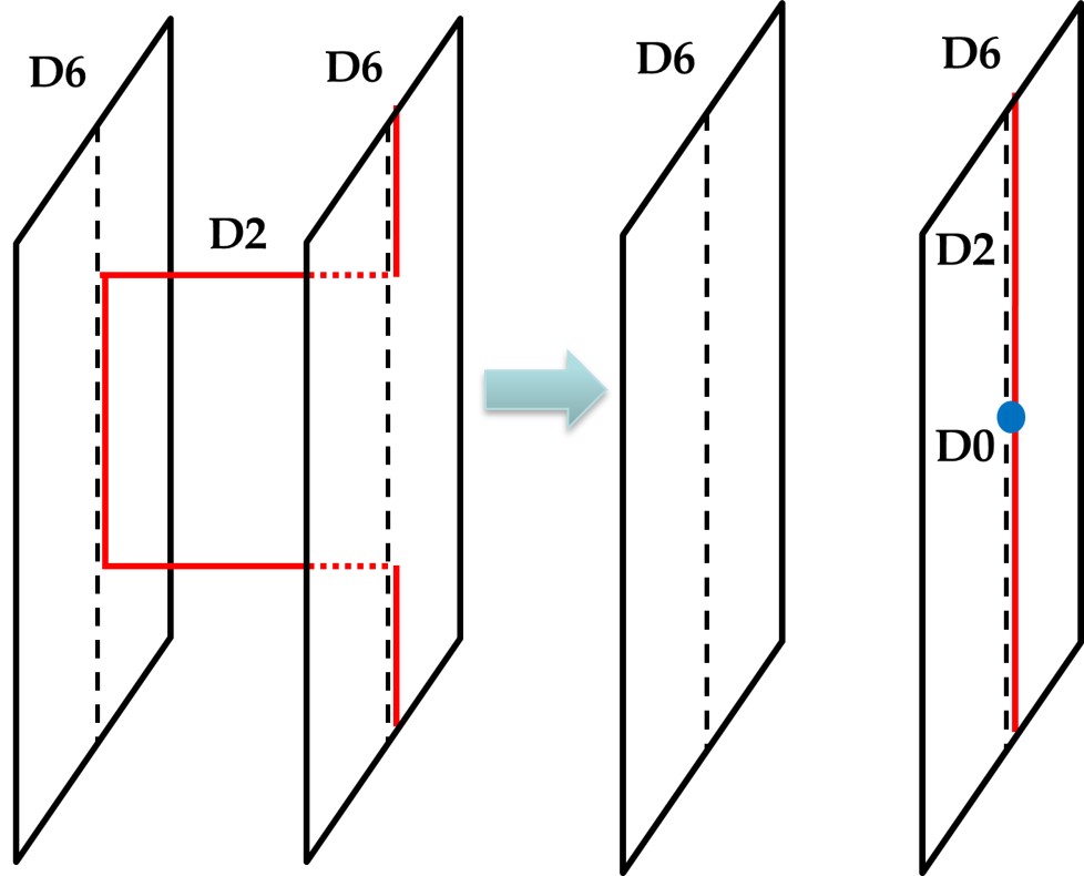
Figure 15: A pair annihilation of kinky D2-brane and anti-kinky D2-brane resulting in the creation of D0-branes.

Consequently, there appear D0-branes afeter the pair annihilation as in Fig. 15 (right). These are nothing but magnetic skyrmions. A pair annihilation of domain wall and anti-domain wall resulting in the creation of magnetic skyrmions. This process was studied in the $O(3)$ model without the DM term Nitta:2012kj ; Nitta:2012kk and Bose-Einstein condensates Takeuchi:2012ee ; Takeuchi:2012ap ; Nitta:2012hy ; Takeuchi:2011uyb . In these cases, the $U(1)$ moduli exist on the domain walls (see footnote 7), and the creation rate of skyrmions depends on the relative phase. The creation rate is maximized when the relative phase moduli is $\pi$, which is precisely the case with the DM term.

Let us make comments on the stability of configurations studied in this paper. In the nonlinear sigma model limit $g\to\infty$, the configurations are known to be stable. At finite coupling $g$, the theory is a gauge theory. The stability analysis in this case has not been studied before and remains an important open question. Finally, in string theory, we expect the stability should be the same with that of the gauge theory, as far as we are considering the field theory limit. However, the most subtle point is that the background gauge field on the flavor D-branes breaks SUSY. As far as we turn on small $\kappa$, the configurations are expected to be stable but the full analysis of this problem is beyond the scope of this paper. The previous studies Bachas:1995ik ; Berkooz:1996km ; Blumenhagen:2000wh ; Angelantonj:2000hi ; Cremades:2004wa ; Kikuchi:2023awm ; Abe:2021uxb on magnetized D-branes in simpler setups should be useful for this purpose. We will come back to this problem in future.

Generalizations of chiral magnets to the ${\mathbb{C}}P^{2}$ model or more generally to the ${\mathbb{C}}P^{N-1}$ model were studied before Akagi:2021dpk ; Akagi:2021lva ; Amari:2022boe in which magnetic skyrmions were mainly investigated. On the other hand, multiple domain walls were studied without the DM interaction in the ${\mathbb{C}}P^{N-1}$ model Gauntlett:2000ib ; Tong:2002hi and Grassmann model Isozumi:2004jc ; Isozumi:2004va ; Isozumi:2004vg , for which multiple kinky D-brane configurations were explored in Ref. Eto:2004vy . Domain-wall skyrmions were also constructed without the DM interaction in parallel multiple walls in the ${\mathbb{C}}P^{N-1}$ model Fujimori:2016tmw and a single non-Abelian domain wall in the Grassmann model Nitta:2015mma ; Nitta:2015mxa . Furthermore, domain wall junctions or networks Eto:2005cp ; Eto:2005fm ; Eto:2006bb ; Eto:2007uc ; Eto:2020vjm ; Eto:2020cys and their D-brane configurations Eto:2005mx were also studied. Introducing the DM interaction in these models will be interesting to explore because these models, at least the ${\mathbb{C}}P^{2}$ model, can be experimentally realizable in laboratory experiments of ultracold atomic gases.

Finally, modulated ground states (vacua) were discussed in string theory Nakamura:2009tf ; Andrade:2015iyf ; Andrade:2017leb ; Andrade:2017cnc ; Cai:2017qdz and relativistic field theory Nitta:2017mgk ; Nitta:2017yuf ; Gudnason:2018bqb ; BjarkeGudnason:2018aij ; Musso:2018wbv . These studies may be useful for analyzing various aspects of the modulated phases found in this paper, for instance phonons in the CSL.

Appendix A The Dzyaloshinskii-Moriya interaction as a background gauge field

In this Appendix, we show that the $SU(2)$ gauged $O(3)$ nonlinear sigma model in Eq. (2.11) can be derived from the strong coupling limit of the $U(1)\times SU(2)$ gauged linear sigma model given in Eq. (2.9), i.e.,

$$\mathcal{L}=2\left({\cal D}_{\mu}\Phi\right)^{\dagger}\left({\cal D}^{\mu}\Phi\right)-\Phi^{\dagger}(\Sigma\mathbf{1}_{2}-M)^{2}\Phi$$ (A.1)

with ${\cal D}_{\mu}\Phi=\left({\partial}_{\mu}-ia_{\mu}-\frac{i}{2}{A}_{\mu}\right)\Phi$ and a $U(1)$ auxiliary gauge field $a_{\mu}$. Since the Lagrangian does not contain the kinetic term of $a_{\mu}$ and $\Sigma$ in the strong coupling limit, they are auxiliary fields. Similar to the case in which $A_{\mu}$ is absent given in Eq. (2.3), one can eliminate the fields using the equations of motion as

$$a_{\mu}=\frac{i}{2}\left\{(\mathscr{D}_{\mu}\Phi)^{\dagger}\Phi-\Phi^{\dagger}(\mathscr{D}_{\mu}\Phi)\right\},\qquad\Sigma=\Phi^{\dagger}M\Phi=mn_{3}$$ (A.2)

with $\mathscr{D}_{\mu}\equiv\partial_{\mu}-\frac{i}{2}{A}_{\mu}$. Substituting them into the Lagrangian in Eq. (A.1), we obtain

$$\mathcal{L} =2\left\{\left(\mathscr{D}_{\mu}\Phi\right)^{\dagger}\left(\mathscr{D}^{\mu}\Phi\right)+\left(\Phi^{\dagger}\mathscr{D}_{\mu}\Phi\right)^{2}\right\}-m^{2}(1-n_{3}^{2})\ .$$ (A.3)

By expanding the expression, we can rewrite the Lagrangian as

$$\begin{split}{\cal L}=&2\left\{\partial_{\mu}\Phi^{\dagger}\partial^{\mu}\Phi+(\Phi^{\dagger}\partial_{\mu}\Phi)\right\}\\ &+i\Phi^{\dagger}A_{\mu}\partial^{\mu}\Phi-i\partial^{\mu}\Phi^{\dagger}A_{\mu}\Phi-2i\Phi^{\dagger}A_{\mu}\Phi\Phi^{\dagger}\partial^{\mu}\Phi\\ &+\frac{1}{2}\left\{(A_{\mu}^{a})^{2}-(\Phi^{\dagger}A_{\mu}\Phi)^{2}\right\}-m^{2}(1-n_{3}^{2})\ .\end{split}$$ (A.4)

Here, we have used a relation

$$\Phi^{\dagger}A_{\mu}A^{\mu}\Phi=A_{\mu}^{a}\left(A^{\mu}\right)^{b}\Phi\sigma_{a}\sigma_{b}\Phi=A_{\mu}^{a}\left(A^{\mu}\right)^{b}~{}\Phi(\delta_{ab}\mathbf{1}_{2}+i\varepsilon^{abc}\sigma_{c})\Phi=(A_{\mu}^{a})^{2}\ .$$ (A.5)

We now compare this Lagrangian and the gauged nonlinear sigma model. First, we can write the Dirichlet term as

$${\partial}_{\mu}{\bf n}\cdot{\partial}^{\mu}{\bf n}= (\sigma_{a})_{\alpha\beta}(\sigma_{b})_{\gamma\delta}~{}{\partial}_{\mu}(\Phi^{*}_{\alpha}\Phi_{\beta}){\partial}_{\mu}(\Phi^{*}_{\gamma}\Phi_{\delta})$$

$$= (2\delta_{\alpha\delta}\delta_{\beta\gamma}-\delta_{\alpha\beta}\delta_{\gamma\delta}){\partial}_{\mu}(\Phi^{*}_{\alpha}\Phi_{\beta}){\partial}_{\mu}(\Phi^{*}_{\gamma}\Phi_{\delta})$$

$$= 2{\partial}_{\mu}(\Phi^{*}_{\alpha}\Phi_{\beta}){\partial}_{\mu}(\Phi^{*}_{\beta}\Phi_{\alpha})$$

$$= 4\left\{\partial_{\mu}\Phi^{\dagger}\partial^{\mu}\Phi+(\Phi^{\dagger}\partial_{\mu}\Phi)\right\}\ .$$ (A.6)

The DM interaction can be rewritten as

$$\bm{A}_{\mu}\cdot\left({\bf n}\times\partial^{\mu}{\bf n}\right) =\varepsilon^{abc}A_{\mu}^{a}n_{b}\partial^{\mu}n_{c}$$

$$=\varepsilon^{abc}A_{\mu}^{a}~{}\Phi^{\dagger}\sigma_{b}\Phi~{}\partial^{\mu}\left(\Phi^{\dagger}\sigma_{c}\Phi\right)$$

$$=iA_{\mu}^{a}~{}\Phi^{\dagger}\left(\sigma_{a}\sigma_{b}-\delta_{ab}\mathbf{1}_{2}\right)\Phi~{}\partial^{\mu}\left(\Phi^{\dagger}\sigma_{b}\Phi\right)$$

$$=iA^{a}_{\mu}\Phi^{\dagger}~{}\sigma_{a}\sigma_{b}\Phi~{}\partial^{\mu}\left(\Phi^{\dagger}\sigma_{b}\Phi\right)-i~{}\partial^{\mu}\left(\Phi^{\dagger}{A}_{\mu}\Phi\right)$$ (A.7)

where we have used $\varepsilon^{abc}\sigma_{c}=-i\left(\sigma_{a}\sigma_{b}-\delta_{ab}\mathbf{1}_{2}\right)$. Using the relation $(\sigma_{a})_{\alpha\beta}(\sigma_{a})_{\gamma\delta}=(2\delta_{\alpha\delta}\delta_{\beta\gamma}-\delta_{\alpha\beta}\delta_{\gamma\delta})$, one obtains

$$\Phi^{\dagger}\sigma_{a}\sigma_{b}\Phi\Phi^{\dagger}\sigma_{b}\partial_{\mu}\Phi =\left(\Phi^{\dagger}\sigma_{a}\right)_{\alpha}(\sigma_{b})_{\alpha\beta}\Phi_{\beta}~{}\Phi_{\gamma}^{\dagger}(\sigma_{b})_{\gamma\delta}\partial_{\mu}\Phi_{\delta}$$

$$=\left(2\delta_{\alpha\delta}\delta_{\beta\gamma}-\delta_{\alpha\beta}\delta_{\gamma\delta}\right)\left(\Phi^{\dagger}\sigma_{a}\right)_{\alpha}\Phi_{\beta}~{}\Phi_{\gamma}^{\dagger}\partial_{\mu}\Phi_{\delta}$$

$$=2\Phi^{\dagger}\sigma_{a}\partial_{k}\Phi-\Phi^{\dagger}\sigma_{a}\Phi~{}\Phi^{\dagger}\partial_{\mu}\Phi$$ (A.8)

and

$$\Phi^{\dagger}\sigma_{a}\sigma_{b}\Phi~{}\partial_{\mu}\Phi^{\dagger}\sigma_{b}\Phi =(\sigma_{b})_{\alpha\beta}(\sigma_{b})_{\gamma\delta}\left(\Phi^{\dagger}\sigma_{a}\right)_{\alpha}\Phi_{\beta}\partial_{\mu}\Phi_{\gamma}^{\dagger}\Phi_{\delta}$$

$$=\left(2\delta_{\alpha\delta}\delta_{\beta\gamma}-\delta_{\alpha\beta}\delta_{\gamma\delta}\right)\left(\Phi^{\dagger}\sigma_{a}\right)_{\alpha}\Phi_{\beta}\partial_{\mu}\Phi^{\dagger}\Phi_{\delta}$$

$$=2\Phi^{\dagger}\sigma_{a}\Phi\partial_{\mu}\Phi^{\dagger}\Phi-\Phi^{\dagger}\sigma_{a}\Phi\partial_{\mu}\Phi^{\dagger}\Phi$$

$$=\Phi^{\dagger}\sigma_{a}\Phi\partial_{\mu}\Phi^{\dagger}\Phi\ .$$ (A.9)

Combining them, we can rewrite the DM interaction as

$$\bm{A}_{\mu}\cdot\left({\bf n}\times\partial^{\mu}{\bf n}\right)= i\left\{2\Phi^{\dagger}{A}_{\mu}\partial^{\mu}\Phi-\Phi^{\dagger}{A}_{\mu}\Phi\Phi^{\dagger}\partial^{\mu}\Phi+\Phi^{\dagger}{A}_{\mu}\Phi\partial^{\mu}\Phi^{\dagger}\Phi\right\}-i\partial^{\mu}\left(\Phi^{\dagger}{A}_{\mu}\Phi\right)$$

$$= i\Phi^{\dagger}{A}_{\mu}\partial^{\mu}\Phi-i\partial^{\mu}\Phi^{\dagger}{A}_{\mu}\Phi-2i\Phi^{\dagger}{A}_{\mu}\Phi\Phi^{\dagger}\partial^{\mu}\Phi\ ,$$ (A.10)

where we have used ${\partial}_{\mu}\Phi^{\dagger}\Phi=-\Phi^{\dagger}{\partial}_{\mu}\Phi$. In addition, we have

$$(\bm{A}_{\mu}\times{\bf n})^{2}=|\bm{A}_{\mu}|^{2}|{\bf n}|^{2}-(\bm{A}_{\mu}\cdot{\bf n})^{2}=(A_{\mu}^{a})^{2}-(\Phi^{\dagger}A_{\mu}\Phi)^{2}\ .$$ (A.11)

We finally find from Eqs. (A.4), (A.6), (A.10) and (A.11) that the $U(1)\times SU(2)$ gauged linear sigma model given in Eq. (2.9) reduces in the strong coupling limit to the $SU(2)$ gauged $O(3)$ nonlinear sigma model in Eq. (2.11).

References

- (1) I. Dzyaloshinskii, A Thermodynamic Theory of ‘Weak’ Ferromagnetism of Antiferromagnetics, J. Phys. Chem. Solids 4 (1958) 241.
- (2) T. Moriya, Anisotropic Superexchange Interaction and Weak Ferromagnetism, Phys. Rev. 120 (1960) 91.
- (3) Y. Togawa, T. Koyama, K. Takayanagi, S. Mori, Y. Kousaka, J. Akimitsu et al., Chiral magnetic soliton lattice on a chiral helimagnet, Phys. Rev. Lett. 108 (2012) 107202.
- (4) Y. Togawa, Y. Kousaka, K. Inoue and J.-I. Kishine, Symmetry, structure, and dynamics of monoaxial chiral magnets, J. Phys. Soc. Jpn. 85 (2016) 112001.
- (5) J. ichiro Kishine and A. Ovchinnikov, Chapter one - theory of monoaxial chiral helimagnet, vol. 66 of Solid State Physics, pp. 1–130, Academic Press, (2015), DOI.
- (6) A. A. Tereshchenko, A. S. Ovchinnikov, I. Proskurin, E. V. Sinitsyn and J.-I. Kishine, Theory of magnetoelastic resonance in a monoaxial chiral helimagnet, Phys. Rev. B 97 (2018) 184303.
- (7) J. Chovan, N. Papanicolaou and S. Komineas, Intermediate phase in the spiral antiferromagnet , Phys. Rev. B 65 (2002) 064433.
- (8) C. Ross and M. Sakai, N.and Nitta, Exact ground states and domain walls in one dimensional chiral magnets, JHEP 12 (2021) 163 [2012.08800].
- (9) A. Bogdanov and D. Yablonskii, Thermodynamically stable vortices in magnetically ordered crystals. The mixed state of magnets, Sov. Phys. JETP 68 (1989) 101.
- (10) A. Bogdanov, New localized solutions of the nonlinear field equations, JETP Lett. 62 (1995) 247.
- (11) S. Mühlbauer, B. Binz, F. Jonietz, C. Pfleiderer, A. Rosch, A. Neubauer et al., Skyrmion lattice in a chiral magnet, Science 323 (2009) 915.
- (12) X. Z. Yu, Y. Onose, N. Kanazawa, J. H. Park, J. H. Han, Y. Matsui et al., Real-space observation of a two-dimensional skyrmion crystal, Nature 465 (2010) 901.
- (13) S. Heinze, K. von Bergmann, M. Menzel, J. Brede, A. Kubetzka, R. Wiesendanger et al., Spontaneous atomic-scale magnetic skyrmion lattice in two dimensions, Nat. Phys. 7 (2011) 713.
- (14) U. K. Rossler, A. N. Bogdanov and C. Pfleiderer, Spontaneous skyrmion ground states in magnetic metals, Nature 442 (2006) 797.
- (15) J. H. Han, J. Zang, Z. Yang, J.-H. Park and N. Nagaosa, Skyrmion Lattice in Two-Dimensional Chiral Magnet, Phys. Rev. B 82 (2010) 094429 [1006.3973].
- (16) S.-Z. Lin, A. Saxena and C. D. Batista, Skyrmion fractionalization and merons in chiral magnets with easy-plane anisotropy, Phys. Rev. B 91 (2015) 224407 [1406.1422].
- (17) C. Ross and M. Nitta, Domain-wall skyrmions in chiral magnets, Phys. Rev. B 107 (2023) 024422 [2205.11417].
- (18) T. Kurumaji, T. Nakajima, M. Hirschberger, A. Kikkawa, Y. Yamasaki, H. Sagayama et al., Skyrmion lattice with a giant topological Hall effect in a frustrated triangular-lattice magnet, Science 365 (2019) 914.
- (19) M. Hirschberger, T. Nakajima, S. Gao, L. Peng, A. Kikkawa, T. Kurumaji et al., Skyrmion phase and competing magnetic orders on a breathing kagomé lattice, Nat. Commun. 10 (2019) 5831.
- (20) N. D. Khanh, T. Nakajima, X. Yu, S. Gao, K. Shibata, M. Hirschberger et al., Nanometric square skyrmion lattice in a centrosymmetric tetragonal magnet, Nat. Nanotechnol. 15 (2020) 444.
- (21) Y. Yasui, C. J. Butler, N. D. Khanh, S. Hayami, T. Nomoto, T. Hanaguri et al., Imaging the coupling between itinerant electrons and localised moments in the centrosymmetric skyrmion magnet , Nat. Commun. 11 (2020) 5925.
- (22) A. Fert, V. Cros and J. Sampaio, Skyrmions on the track, Nat. Nanotechnol. 8 (2013) 152.
- (23) N. Nagaosa and Y. Tokura, Topological properties and dynamics of magnetic skyrmions, Nat. Nanotechnol. 8 (2013) 899–911.
- (24) M. Nitta, Josephson vortices and the Atiyah-Manton construction, Phys. Rev. D 86 (2012) 125004 [1207.6958].
- (25) M. Kobayashi and M. Nitta, Sine-Gordon kinks on a domain wall ring, Phys. Rev. D 87 (2013) 085003 [1302.0989].
- (26) R. Auzzi, M. Shifman and A. Yung, Domain Lines as Fractional Strings, Phys. Rev. D 74 (2006) 045007 [hep-th/0606060].
- (27) P. Jennings and P. Sutcliffe, The dynamics of domain wall Skyrmions, J. Phys. A 46 (2013) 465401 [1305.2869].
- (28) V. Bychkov, M. Kreshchuk and E. Kurianovych, Strings and skyrmions on domain walls, Int. J. Mod. Phys. A 33 (2018) 1850111 [1603.06310].
- (29) M. Eto, M. Nitta, K. Ohashi and D. Tong, Skyrmions from instantons inside domain walls, Phys. Rev. Lett. 95 (2005) 252003 [hep-th/0508130].
- (30) M. Nitta, Correspondence between Skyrmions in 2+1 and 3+1 Dimensions, Phys. Rev. D 87 (2013) 025013 [1210.2233].
- (31) M. Nitta, Matryoshka Skyrmions, Nucl. Phys. B 872 (2013) 62 [1211.4916].
- (32) S. B. Gudnason and M. Nitta, Domain wall Skyrmions, Phys. Rev. D 89 (2014) 085022 [1403.1245].
- (33) S. B. Gudnason and M. Nitta, Incarnations of Skyrmions, Phys. Rev. D 90 (2014) 085007 [1407.7210].
- (34) M. Eto and M. Nitta, Non-Abelian Sine-Gordon Solitons: Correspondence between Skyrmions and Lumps, Phys. Rev. D 91 (2015) 085044 [1501.07038].
- (35) M. Eto, K. Nishimura and M. Nitta, How baryons appear in low-energy QCD: Domain-wall Skyrmion phase in strong magnetic fields, 2304.02940.
- (36) M. Eto, K. Nishimura and M. Nitta, Phase diagram of QCD matter with magnetic field: domain-wall Skyrmion chain in chiral soliton lattice, 2311.01112.
- (37) M. Eto, K. Nishimura and M. Nitta, Domain-wall Skyrmion phase in a rapidly rotating QCD matter, 2310.17511.
- (38) S. Lepadatu, Emergence of transient domain wall skyrmions after ultrafast demagnetization, Phys. Rev. B 102 (2020) 094402.
- (39) T.Nagase, Y.-G. So, H. Yasui, T. Ishida, H. K. Yoshida, Y. Tanaka et al., Observation of domain wall bimerons in chiral magnets, Nat. Commun. 12 (2021) 3490 [2004.06976].
- (40) K. Yang, K. Nagase and Y. Hirayama et.al., Wigner solids of domain wall skyrmions, Nat. Commun. 12 (2021) 6006.
- (41) S. K. Kim and Y. Tserkovnyak, Magnetic Domain Walls as Hosts of Spin Superfluids and Generators of Skyrmions, Phys. Rev. Lett. 119 (2017) 047202 [1701.08273].
- (42) R. Cheng, M. Li, A. Sapkota, A. Rai, A. Pokhrel, T. Mewes et al., Magnetic domain wall skyrmions, Phys. Rev. B 99 (2019) 184412.
- (43) V. M. Kuchkin, B. Barton-Singer, F. N. Rybakov, S. Blügel, B. J. Schroers and N. S. Kiselev, Magnetic skyrmions, chiral kinks and holomorphic functions, Phys. Rev. B 102 (2020) 144422 [2007.06260].
- (44) T. Tanigaki, K. Shibata, N. Kanazawa, X. Yu, Y. Onose, H. S. Park et al., Real-Space Observation of Short-Period Cubic Lattice of Skyrmions in MnGe, Nano Lett. 15 (2015) 5438.
- (45) Y. Fujishiro, N. Kanazawa, T. Nakajima, X. Yu, K. Ohishi, Y. Kawamura et al., Topological transitions among skyrmion- and hedgehog-lattice states in cubic chiral magnets, Nat. Commun. 10 (2019) 1059.
- (46) P. Sutcliffe, Hopfions in chiral magnets, J. Phys. A 51 (2018) 375401 [1806.06458].
- (47) M. Hongo, T. Fujimori, T. Misumi, M. Nitta and N. Sakai, Instantons in Chiral Magnets, Phys. Rev. B 101 (2020) 104417 [1907.02062].
- (48) B. Göbel, I. Mertig and O. A. Tretiakov, Beyond skyrmions: Review and perspectives of alternative magnetic quasiparticles, Phys. Rep. 895 (2021) 1.
- (49) B. Barton-Singer, C. Ross and B. J. Schroers, Magnetic Skyrmions at Critical Coupling, Commun. Math. Phys. 375 (2020) 2259 [1812.07268].
- (50) B. J. Schroers, Gauged Sigma Models and Magnetic Skyrmions, SciPost Phys. 7 (2019) 030 [1905.06285].
- (51) C. Ross, N. Sakai and M. Nitta, Skyrmion interactions and lattices in chiral magnets: analytical results, JHEP 02 (2021) 095 [2003.07147].
- (52) A. Hanany and E. Witten, Type IIB superstrings, BPS monopoles, and three-dimensional gauge dynamics, Nucl. Phys. B 492 (1997) 152 [hep-th/9611230].
- (53) A. Giveon and D. Kutasov, Brane Dynamics and Gauge Theory, Rev. Mod. Phys. 71 (1999) 983 [hep-th/9802067].
- (54) C. Bachas, A Way to break supersymmetry, hep-th/9503030.
- (55) M. Berkooz, M. R. Douglas and R. G. Leigh, Branes intersecting at angles, Nucl. Phys. B 480 (1996) 265 [hep-th/9606139].
- (56) R. Blumenhagen, L. Goerlich, B. Kors and D. Lust, Noncommutative compactifications of type I strings on tori with magnetic background flux, JHEP 10 (2000) 006 [hep-th/0007024].
- (57) C. Angelantonj, I. Antoniadis, E. Dudas and A. Sagnotti, Type I strings on magnetized orbifolds and brane transmutation, Phys. Lett. B 489 (2000) 223 [hep-th/0007090].
- (58) D. Cremades, L. E. Ibanez and F. Marchesano, Computing Yukawa couplings from magnetized extra dimensions, JHEP 05 (2004) 079 [hep-th/0404229].
- (59) S. Kikuchi, T. Kobayashi, K. Nasu, S. Takada and H. Uchida, Zero-modes in magnetized orbifold models through modular symmetry, 2305.16709.
- (60) Y. Abe, T. Higaki, T. Kobayashi, S. Takada and R. Takahashi, 4D effective action from the non-Abelian DBI action with a magnetic flux background, Phys. Rev. D 104 (2021) 126020 [2107.11961].
- (61) N. D. Lambert and D. Tong, Kinky D strings, Nucl. Phys. B 569 (2000) 606 [hep-th/9907098].
- (62) M. Eto, Y. Isozumi, M. Nitta, K. Ohashi, K. Ohta and N. Sakai, D-brane construction for non-Abelian walls, Phys. Rev. D 71 (2005) 125006 [hep-th/0412024].
- (63) M. Eto, T. Fujimori, Y. Isozumi, M. Nitta, K. Ohashi, K. Ohta et al., Non-Abelian vortices on cylinder: Duality between vortices and walls, Phys. Rev. D 73 (2006) 085008 [hep-th/0601181].
- (64) M. Eto, T. Fujimori, M. Nitta, K. Ohashi, K. Ohta and N. Sakai, Statistical mechanics of vortices from D-branes and T-duality, Nucl. Phys. B 788 (2008) 120 [hep-th/0703197].
- (65) T. Misumi, M. Nitta and N. Sakai, Classifying bions in Grassmann sigma models and non-Abelian gauge theories by D-branes, Prog. Theor. Exp. Phys. 2015 (2015) 033B02 [1409.3444].
- (66) A. Hanany and D. Tong, Vortices, instantons and branes, JHEP 07 (2003) 037 [hep-th/0306150].
- (67) M. Nitta, Relations among topological solitons, Phys. Rev. D 105 (2022) 105006 [2202.03929].
- (68) M. Eto, Y. Isozumi, M. Nitta, K. Ohashi and N. Sakai, Solitons in the Higgs phase: The Moduli matrix approach, J. Phys. A 39 (2006) R315 [hep-th/0602170].
- (69) A. Hanany and D. Tong, Vortex strings and four-dimensional gauge dynamics, JHEP 04 (2004) 066 [hep-th/0403158].
- (70) M. Arai, M. Nitta and N. Sakai, Vacua of massive hyper-Kahler sigma models of non-Abelian quotient, Prog. Theor. Phys. 113 (2005) 657 [hep-th/0307274].
- (71) P. Kronheimer and H. Nakajima, Yang-Mills instantons on ALE gravitational instantons, Math. Ann. (1990) 263–307.
- (72) D. T. Son and M. A. Stephanov, Axial anomaly and magnetism of nuclear and quark matter, Phys. Rev. D 77 (2008) 014021 [0710.1084].
- (73) T. Brauner and N. Yamamoto, Chiral Soliton Lattice and Charged Pion Condensation in Strong Magnetic Fields, JHEP 04 (2017) 132 [1609.05213].
- (74) K. Nishimura and N. Yamamoto, Topological term, QCD anomaly, and the chiral soliton lattice in rotating baryonic matter, JHEP 07 (2020) 196 [2003.13945].
- (75) M. Eto, K. Nishimura and M. Nitta, Phases of rotating baryonic matter: non-Abelian chiral soliton lattices, antiferro-isospin chains, and ferri/ferromagnetic magnetization, JHEP 08 (2022) 305 [2112.01381].
- (76) D. T. Son and A. R. Zhitnitsky, Quantum anomalies in dense matter, Phys. Rev. D 70 (2004) 074018 [hep-ph/0405216].
- (77) E. R. C. Abraham and P. K. Townsend, Q kinks, Phys. Lett. B 291 (1992) 85.
- (78) M. Arai, M. Naganuma, M. Nitta and N. Sakai, Manifest supersymmetry for BPS walls in N=2 nonlinear sigma models, Nucl. Phys. B 652 (2003) 35 [hep-th/0211103].
- (79) M. Arai, M. Naganuma, M. Nitta and N. Sakai, BPS wall in N=2 SUSY nonlinear sigma model with Eguchi-Hanson manifold, hep-th/0302028.
- (80) A. Hanany and D. Tong, On monopoles and domain walls, Commun. Math. Phys. 266 (2006) 647 [hep-th/0507140].
- (81) R. Auzzi, S. Bolognesi, J. Evslin, K. Konishi and A. Yung, NonAbelian superconductors: Vortices and confinement in N=2 SQCD, Nucl. Phys. B 673 (2003) 187 [hep-th/0307287].
- (82) M. Eto, Y. Isozumi, M. Nitta, K. Ohashi and N. Sakai, Moduli space of non-Abelian vortices, Phys. Rev. Lett. 96 (2006) 161601 [hep-th/0511088].
- (83) M. Eto, K. Konishi, G. Marmorini, M. Nitta, K. Ohashi, W. Vinci et al., Non-Abelian Vortices of Higher Winding Numbers, Phys. Rev. D 74 (2006) 065021 [hep-th/0607070].
- (84) M. Shifman and A. Yung, Supersymmetric Solitons and How They Help Us Understand Non-Abelian Gauge Theories, Rev. Mod. Phys. 79 (2007) 1139 [hep-th/0703267].
- (85) M. Shifman and A. Yung, Supersymmetric solitons, Cambridge Monographs on Mathematical Physics. Cambridge University Press, 5, 2009.
- (86) M. Eto, Y. Isozumi, M. Nitta, K. Ohashi and N. Sakai, Instantons in the Higgs phase, Phys. Rev. D 72 (2005) 025011 [hep-th/0412048].
- (87) A. A. Abrikosov, On the Magnetic properties of superconductors of the second group, Sov. Phys. JETP 5 (1957) 1174.
- (88) H. B. Nielsen and P. Olesen, Vortex Line Models for Dual Strings, Nucl. Phys. B 61 (1973) 45.
- (89) T. Vachaspati and A. Achucarro, Semilocal cosmic strings, Phys. Rev. D 44 (1991) 3067.
- (90) A. Achucarro and T. Vachaspati, Semilocal and electroweak strings, Phys. Rept. 327 (2000) 347 [hep-ph/9904229].
- (91) M. Shifman and A. Yung, Non-Abelian semilocal strings in N=2 supersymmetric QCD, Phys. Rev. D 73 (2006) 125012 [hep-th/0603134].
- (92) M. Eto, J. Evslin, K. Konishi, G. Marmorini, M. Nitta, K. Ohashi et al., On the moduli space of semilocal strings and lumps, Phys. Rev. D 76 (2007) 105002 [0704.2218].
- (93) Y. M. Shnir, Topological and Non-Topological Solitons in Scalar Field Theories, Cambridge Monographs on Mathematical Physics. Cambridge University Press, Cambridge, 2018.
- (94) Y. Amari, C. Ross and M. Nitta, Domain-wall skyrmion chain and domain-wall bimerons in chiral magnets, 2311.05174.
- (95) P. G. de Gennes, Phase Transition and Turbulence: An Introduction, pp. 1–18. Springer US, Boston, MA, 1975. 10.1007/978-1-4615-8912-9_1.
- (96) Y. Masaki, Instabilities in monoaxial chiral magnets under a tilted magnetic field, Phys. Rev. B 101 (2020) 214424.
- (97) M. Eto and M. Nitta, Quantum nucleation of topological solitons, JHEP 09 (2022) 077 [2207.00211].
- (98) T. Higaki, K. Kamada and K. Nishimura, Formation of a chiral soliton lattice, Phys. Rev. D 106 (2022) 096022 [2207.00212].
- (99) A. Sen, Tachyon condensation on the brane anti-brane system, JHEP 08 (1998) 012 [hep-th/9805170].
- (100) A. Sen, Tachyon dynamics in open string theory, Int. J. Mod. Phys. A 20 (2005) 5513 [hep-th/0410103].
- (101) M. Nitta, Defect formation from defect–anti-defect annihilations, Phys. Rev. D 85 (2012) 101702 [1205.2442].
- (102) M. Nitta, Knots from wall–anti-wall annihilations with stretched strings, Phys. Rev. D 85 (2012) 121701 [1205.2443].
- (103) H. Takeuchi, K. Kasamatsu, M. Tsubota and M. Nitta, Tachyon Condensation Due to Domain-Wall Annihilation in Bose-Einstein Condensates, Phys. Rev. Lett. 109 (2012) 245301 [1205.2330].
- (104) H. Takeuchi, K. Kasamatsu, M. Tsubota and M. Nitta, Tachyon Condensation and Brane Annihilation in Bose-Einstein Condensates: Spontaneous Symmetry Breaking in Restricted Lower-dimensional Subspace, J. Low Temp. Phys. 171 (2013) 443 [1211.3952].
- (105) M. Nitta, K. Kasamatsu, M. Tsubota and H. Takeuchi, Creating vortons and three-dimensional skyrmions from domain wall annihilation with stretched vortices in Bose-Einstein condensates, Phys. Rev. A 85 (2012) 053639 [1203.4896].
- (106) H. Takeuchi, K. Kasamatsu, M. Nitta and M. Tsubota, Vortex Formations from Domain Wall Annihilations in Two-component Bose-Einstein Condensates, J. Low Temp. Phys. 162 (2011) 243 [1205.2328].
- (107) Y. Akagi, Y. Amari, N. Sawado and Y. Shnir, Isolated skyrmions in the nonlinear sigma model with a Dzyaloshinskii-Moriya type interaction, Phys. Rev. D 103 (2021) 065008 [2101.10566].
- (108) Y. Akagi, Y. Amari, S. B. Gudnason, M. Nitta and Y. Shnir, Fractional Skyrmion molecules in a model, JHEP 11 (2021) 194 [2107.13777].
- (109) Y. Amari, Y. Akagi, S. B. Gudnason, M. Nitta and Y. Shnir, skyrmion crystals in an SU(3) magnet with a generalized Dzyaloshinskii-Moriya interaction, Phys. Rev. B 106 (2022) L100406 [2204.01476].
- (110) J. P. Gauntlett, D. Tong and P. K. Townsend, Multidomain walls in massive supersymmetric sigma models, Phys. Rev. D 64 (2001) 025010 [hep-th/0012178].
- (111) D. Tong, The Moduli space of BPS domain walls, Phys. Rev. D 66 (2002) 025013 [hep-th/0202012].
- (112) Y. Isozumi, M. Nitta, K. Ohashi and N. Sakai, Construction of non-Abelian walls and their complete moduli space, Phys. Rev. Lett. 93 (2004) 161601 [hep-th/0404198].
- (113) Y. Isozumi, M. Nitta, K. Ohashi and N. Sakai, Non-Abelian walls in supersymmetric gauge theories, Phys. Rev. D 70 (2004) 125014 [hep-th/0405194].
- (114) Y. Isozumi, M. Nitta, K. Ohashi and N. Sakai, All exact solutions of a 1/4 Bogomol’nyi-Prasad-Sommerfield equation, Phys. Rev. D 71 (2005) 065018 [hep-th/0405129].
- (115) T. Fujimori, H. Iida and M. Nitta, Field theoretical model of multilayered Josephson junction and dynamics of Josephson vortices, Phys. Rev. B 94 (2016) 104504 [1604.08103].
- (116) M. Nitta, Josephson junction of non-Abelian superconductors and non-Abelian Josephson vortices, Nucl. Phys. B 899 (2015) 78 [1502.02525].
- (117) M. Nitta, Josephson instantons and Josephson monopoles in a non-Abelian Josephson junction, Phys. Rev. D 92 (2015) 045010 [1503.02060].
- (118) M. Eto, Y. Isozumi, M. Nitta, K. Ohashi and N. Sakai, Webs of walls, Phys. Rev. D 72 (2005) 085004 [hep-th/0506135].
- (119) M. Eto, Y. Isozumi, M. Nitta, K. Ohashi and N. Sakai, Non-Abelian webs of walls, Phys. Lett. B 632 (2006) 384 [hep-th/0508241].
- (120) M. Eto, T. Fujimori, T. Nagashima, M. Nitta, K. Ohashi and N. Sakai, Effective Action of Domain Wall Networks, Phys. Rev. D 75 (2007) 045010 [hep-th/0612003].
- (121) M. Eto, T. Fujimori, T. Nagashima, M. Nitta, K. Ohashi and N. Sakai, Dynamics of Domain Wall Networks, Phys. Rev. D 76 (2007) 125025 [0707.3267].
- (122) M. Eto, M. Kawaguchi, M. Nitta and R. Sasaki, Exact solutions of domain wall junctions in arbitrary dimensions, Phys. Rev. D 102 (2020) 065006 [2001.07552].
- (123) M. Eto, M. Kawaguchi, M. Nitta and R. Sasaki, Exhausting all exact solutions of BPS domain wall networks in arbitrary dimensions, Phys. Rev. D 101 (2020) 105020 [2003.13520].
- (124) M. Eto, Y. Isozumi, M. Nitta, K. Ohashi, K. Ohta and N. Sakai, D-brane configurations for domain walls and their webs, AIP Conf. Proc. 805 (2005) 354 [hep-th/0509127].
- (125) S. Nakamura, H. Ooguri and C.-S. Park, Gravity Dual of Spatially Modulated Phase, Phys. Rev. D 81 (2010) 044018 [0911.0679].
- (126) T. Andrade and A. Krikun, Commensurability effects in holographic homogeneous lattices, JHEP 05 (2016) 039 [1512.02465].
- (127) T. Andrade and A. Krikun, Commensurate lock-in in holographic non-homogeneous lattices, JHEP 03 (2017) 168 [1701.04625].
- (128) T. Andrade, M. Baggioli, A. Krikun and N. Poovuttikul, Pinning of longitudinal phonons in holographic spontaneous helices, JHEP 02 (2018) 085 [1708.08306].
- (129) R.-G. Cai, L. Li, Y.-Q. Wang and J. Zaanen, Intertwined Order and Holography: The Case of Parity Breaking Pair Density Waves, Phys. Rev. Lett. 119 (2017) 181601 [1706.01470].
- (130) M. Nitta, S. Sasaki and R. Yokokura, Spatially Modulated Vacua in a Lorentz-invariant Scalar Field Theory, Eur. Phys. J. C 78 (2018) 754 [1706.02938].
- (131) M. Nitta, S. Sasaki and R. Yokokura, Supersymmetry Breaking in Spatially Modulated Vacua, Phys. Rev. D 96 (2017) 105022 [1706.05232].
- (132) S. B. Gudnason, M. Nitta, S. Sasaki and R. Yokokura, Temporally, spatially, or lightlike modulated vacua in Lorentz invariant theories, Phys. Rev. D 99 (2019) 045011 [1810.11361].
- (133) S. Bjarke Gudnason, M. Nitta, S. Sasaki and R. Yokokura, Supersymmetry breaking and ghost Goldstino in modulated vacua, Phys. Rev. D 99 (2019) 045012 [1812.09078].
- (134) D. Musso, Simplest phonons and pseudo-phonons in field theory, Eur. Phys. J. C 79 (2019) 986 [1810.01799].