Chemical Distribution of the Dynamical Ejecta in the Neutron Star Merger GW170817

Abstract

GW170817 and its associated electromagnetic counterpart AT2017gfo continue to be a treasure trove as observations and modeling continue. Recent precision astrometry of AT2017gfo with the Hubble Space Telescope combined with previous constraints from Very Long Baseline Interferometry (VLBI) constraints narrowed down the inclination angle to 19-25 deg (90% confidence). This paper explores how the inclusion of precise inclination information can reveal new insights about the ejecta properties, in particular, about the composition of the dynamical ejecta of AT2017gfo. Our analysis relies on updated kilonova modeling, which includes state-of-the-art heating rates, thermalization efficiencies, and opacities and is parameterized by $\bar{Y}_{\rm e,dyn}$, the average electron fraction of the dynamical ejecta component. Using this model, we incorporate the latest inclination angle constraint of AT2017gfo into a light curve fitting framework to derive updated parameter estimates. Our results suggest that the viewing angle of the observer is pointed towards the lanthanide-poor ($Y_{\rm e,dyn}\gtrsim 0.25$), squeezed polar dynamical ejecta component, which can explain the early blue emission observed in the light curve of AT2017gfo. In contrast to a recent claim of spherical ejecta powering AT2017gfo, our study indicates that the composition of the dynamical ejecta has a strong angular dependence, with a lanthanide-rich ($Y_{\rm e,dyn}\lesssim 0.25$), tidal component distributed around the merger plane with a half-opening angle of $35^{\circ}$. The inclination angle constraint reduces $\bar{Y}_{\rm e,dyn}$ from $0.24$ to $0.22$, with values $0.17\lesssim Y_{\rm e,dyn}\lesssim 0.41$ enabling the robust production of $r$-process elements up to the $3^{\rm rd}$ peak in the tidal dynamical ejecta.

1 Introduction

More than five years since its discovery, the binary neutron star (BNS) merger GW170817 remains the only gravitational-wave event with a definitive electromagnetic (EM) counterpart (Abbott et al., 2017): a low-luminosity short gamma-ray burst (Goldstein et al., 2017; Savchenko et al., 2017), a kilonova peaking at ultraviolet to infrared wavelengths (Andreoni et al., 2017; Chornock et al., 2017; Coulter et al., 2017; Evans et al., 2017; Kasliwal et al., 2022; Kilpatrick et al., 2017; Lipunov et al., 2017; McCully et al., 2017; Shappee et al., 2017; Tanvir et al., 2017; Utsumi et al., 2017), and a gamma-ray burst (GRB) afterglow with multi-wavelength emission (Margutti et al., 2017; Fong et al., 2019; Lamb et al., 2019). The precise localization of GW170817 to the lenticular galaxy NGC 4993 at 40 Mpc (Coulter et al., 2017) enabled a detailed study of the energetics of the different outflow components, such as the dynamical ejecta, the disk wind ejecta, and the relativistic jet, responsible for the EM counterparts.

Detectable emission from AT2017gfo lasted for a few weeks post-merger. Due to the initially dominant ultraviolet and blue emission, numerical-relativity simulations indicated the presence of at least two components associated with the kilonova: $\sim 0.01M_{\odot}$ of lanthanide-poor ejecta (i.e., blue component) traveling at an average speed of $\sim$0.3c, and $\sim 0.05M_{\odot}$ of lanthanide-rich material (i.e., red component) traveling at $\sim$0.1c (Arcavi et al., 2017; Cowperthwaite et al., 2017; Drout et al., 2017; Kasen et al., 2017; Kasliwal et al., 2017; Nicholl et al., 2017; Pian et al., 2017; Smartt et al., 2017; Soares-Santos et al., 2017; Tanvir et al., 2017; Valenti et al., 2017; Villar et al., 2017). The blue component was interpreted as originating preferentially in the polar regions due to irradiation from neutrinos from a short-lived hypermassive neutron star (HMNS), while the red component to be preferentially equatorial, due to shielding of the neutrinos by the accretion disk (Kasen et al., 2017; Metzger & Fernández, 2014; Metzger, 2019). However, ejecta masses and velocities inferred for these two components did not agree well with those predicted by numerical-relativity simulations (Siegel, 2019). While additional explanations like magnetar-energized wind (Metzger et al., 2018; Yu et al., 2018) have been proposed for the kilonova emission, there is no evidence for a long-lived magnetar in GW170817 (Pooley et al., 2018; Margutti et al., 2018; Makhathini et al., 2021; Kawaguchi et al., 2022; Mooley et al., 2022).

The above general conclusions have been drawn from one-dimensional, inclination-independent analyses. This scenario has changed with the proper motion measurements of the relativistic jet in GW170817, made with the Hubble Space Telescope and very long baseline interferometry (Mooley et al., 2018; Ghirlanda et al., 2019; Mooley et al., 2022), yielding a precise viewing angle constraint of $19<\theta_{\rm obs}<25$ degrees (90% confidence). Precise measurements of the inclination angle of GW170817 can allow for a more accurate inference of the properties of the associated kilonova, including the ejecta masses, velocities, and composition.

In this work, we present inference results using the tight inclination angle constraint for AT2017gfo and show how the inclusion of inclination angle constraints affects the ejecta parameters and in particular the composition of the dynamical ejecta. We employ a new grid based on an improved version (Bulla, 2023) of POSSIS (Bulla, 2019), a three-dimensional Monte Carlo code for modeling the radiation transport in kilonovae. We use idealized outflow properties (geometry and distributions of density and composition) guided by numerical-relativity simulations combined together with the inclination angle constraint.

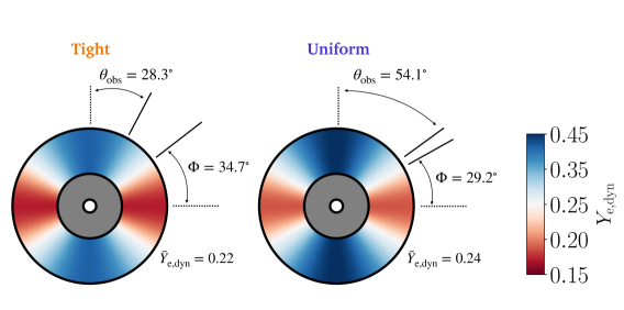
Figure 1: Schematic diagram of the ejecta distribution for AT2017gfo as inferred from the Bu2023Ye grid. The two distinct regions of the dynamical ejecta are represented in blue, corresponding to the lanthanide-poor, squeezed polar dynamical ejecta, and the red, representing the lanthanide-rich, equatorial tidal component. The disk wind ejecta is represented by the grey annulus in the center. The solid lines show the boundary between the lanthanide-rich and lanthanide-poor regions of the dynamical ejecta based on our tight results (left) and our uniform results (right). We quote numbers for $\Phi$, $\bar{Y}_{\rm e,dyn}$, and $\theta_{\rm obs}$. Both runs suggest that the observer is directly viewing the wide-angle, blue polar dynamical ejecta component of AT2017gfo.

2 Methodology

2.1 Kilonova Models

We make use of the three-dimensional, time-dependent Monte Carlo (MC) radiative transfer code POSSIS (Bulla, 2019, 2023) for simulating kilonova light curves. The code simulates the propagation of MC photon packets as they diffuse out of an expanding medium and interact with matter. Each grid cell in the model is assigned a density $\rho$ (evolved with time assuming homologous expansion), an electron fraction $Y_{\rm e}$ (constant throughout the simulation), and a temperature $T$ (estimated from the mean intensity of the radiation field). At the start of the simulation, MC photon packets are assigned an initial location sampled from the distribution of energy from radioactive-decay of $r$-process nuclei (i.e., depending on the mass and heating rates distribution within the model). The energy available at each time-step is estimated from heating rates (Rosswog & Korobkin, 2022) and thermalization efficiencies (Barnes et al., 2016; Wollaeger et al., 2018) that depend on local properties of the ejecta and split equally among MC packets (Lucy, 1999). The propagation of MC packets is controlled by the opacity of the ejecta, which is dominated by bound-bound transitions and electron scattering. The most recent version of POSSIS (Bulla, 2023) uses time-dependent opacities that depend on local properties of the ejecta such as $\rho$, $T$, $Y_{\rm e}$, and on the photon frequency/wavelength in the case of bound-bound transitions (Tanaka et al., 2020). We refer the reader to Bulla (2019) and Bulla (2023) for more details about the code.

In this article, we computed a new kilonova grid based on the BNS ejecta model described in Bulla (2023). The ejecta are modeled following Kawaguchi et al. (2020) and with an idealized geometry assuming two main components: the dynamical ejecta, which is ejected during the merger, and the wind ejecta, which is ejected from the debris disk formed around the central remnant post-merger. The dynamical ejecta, which extend from $0.1$c to $v_{\rm max,dyn}$, where c is the speed of light, have a density profile depending on both the radius $r$ and polar angle $\theta$ as

$$\rho(r,t,\theta)\propto\begin{cases}\,\sin^{2}(\theta)\,r^{-4}\,t^{-3}\,\,,\,\,\,\,0.1c\leq r/t\leq 0.4c\\ \,\sin^{2}(\theta)\,r^{-8}\,t^{-3}\,\,,\,\,\,\,0.4c\leq r/t\leq v_{\rm max,dyn}\end{cases}~{}$$ (1)

and an electron fraction depending on $\theta$ as

$$Y_{\rm e,dyn}(\theta)=a\,\cos^{2}(\theta)\,+\,b.$$ (2)

Specifically, we scale the densities and $v_{\rm max,dyn}$ to achieve a desired mass $M_{\rm ej,dyn}$ and mass-weighted averaged velocity $\bar{v}_{\rm ej,dyn}$, respectively, and assume that the parameters $a$ and $b$ are linked as in Setzer et al. (2023) ($a\sim 0.71\,b$) and $a$ scaled to obtain a desired mass mean-weighted averaged electron fraction $\bar{Y}_{\rm e,dyn}$. The wind ejecta extend from 0.02 to $v_{\rm max,wind}$, with a density profile $\rho(r)\propto r^{-3}\,t^{-3}$ and a fixed electron fraction $Y_{\rm e,wind}=0.3$. The densities and $v_{\rm max,wind}$ are scaled to obtain a desired $M_{\rm ej,wind}$ and mass-weighted averaged velocity $\bar{v}_{\rm ej,wind}$, respectively. If $v_{\rm max,wind}>0.1$c (i.e., the minimum velocity of the dynamical ejecta), we follow Kawaguchi et al. (2020) and assume that the wind ejecta replaces the dynamical ejecta at velocities larger than 0.1c and for angles $\theta<\pi/4$ (see, e.g., their Fig. 2, bottom panel).

The new kilonova grid, hereafter referred to as Bu2023Ye, depends on five free parameters in addition to the viewing angle $\Theta_{\rm obs}$: $M_{\rm ej,dyn}$, $\bar{v}_{\rm ej,dyn}$, $\bar{Y}_{\rm e,dyn}$, $M_{\rm ej,wind}$, and $\bar{v}_{\rm ej,wind}$. Values for these parameters are chosen to cover the expected ranges from numerical-relativity simulations of binary neutron star mergers (e.g. Radice et al., 2018; Nedora et al., 2021b): $M_{\rm ej,dyn}=[0.001,0.005,0.010,0.020]\,M_{\odot}$, $\bar{v}_{\rm ej,dyn}=[0.12,0.15,0.20,0.25]$c, $\bar{Y}_{\rm e,dyn}=[0.15,0.20,0.25,0.3]$, $M_{\rm ej,wind}=[0.01,0.05,0.09,0.13]\,M_{\odot}$ and $\bar{v}_{\rm ej,wind}=[0.03,0.05,0.10,0.15]$c. This results in a total of $4\times 4\times 4\times 4\times 4=1024$ configurations, corresponding to $11264$ different kilonova light curves when counting the $N_{\rm obs}=11$ different viewing angles $\theta_{\rm obs}$ (equally spaced in cosine from a face-on / jet-axis to an edge-on / merger-plane view of the system). Each simulation employs a number $N_{\rm ph}=10^{6}$ of MC photon packets, $N_{\rm times}=100$ time-steps from $0.1$ to $30$ d after the merger (logarithmic binning of $\Delta\log t=0.025$) and $N_{\rm\lambda}=1000$ wavelength bins from $500$ Å to $10\,\mu$m (logarithmic binning of $\Delta\log\lambda=0.0023$).

For comparison, we also make use of the grid introduced in Dietrich et al. (2020), parameterized by $M_{\rm ej,dyn}$, $M_{\rm ej,wind}$, $\Phi$, and $\theta_{\rm obs}$. This kilonova grid uses an earlier version of POSSIS (Bulla, 2019) with analytic functions for the opacities and simpler prescriptions for heating rates and thermalization efficiencies. In the rest of the paper, the model built upon the old grid, Dietrich et al. (2020), is referred to as Bu2019lm.

Fig. 1 shows a sketch of the ejecta for the best-fit model found in this work. We note that the constraint on the averaged $\bar{Y}_{\rm e,dyn}$, coupled with the $Y_{\rm e,dyn}(\theta)$ angular dependence in Eq. (2), leads to a constraint on the chemical distribution of the dynamical ejecta and specifically on the half-opening angle $\Phi$ of the lanthanide-rich ($Y_{\rm e}<0.25$) region, see below.

2.2 Bayesian analysis using NMMA

To analyse AT2017gfo, we use the Nuclear physics and Multi-Messenger Astronomy framework NMMA (Dietrich et al., 2020; Pang et al., 2022) that allows us to perform joint Bayesian inference of multi-messenger events containing gravitational waves, kilonovae, supernovae, and GRB afterglows.

To perform Bayesian analysis on the light curve data using the grid of predicted light curves, an interpolation scheme is required. Here, we employ a feed-forward neural network (NN) to predict the kilonova light curves based on the input parameters (Almualla et al., 2021). We used a NN to create a continuous mapping between merger parameters and light curve eigenvalues. The NN architecture begins with an input layer followed by one dense layer with 2048 neurons. A dropout layer subsequently removes 60% of the dense layer’s outputs before connecting to the output layer, yielding ten eigenvalues. This regularized, wide and shallow NN approximates a Gaussian process (see e.g., Lee et al. 2017) in a fraction of its runtime. We used 90% of learning set examples to train the models over 100 epochs, reserving the remaining 10% for validation.

The inference of kilonovae is based on the AB magnitude for a specific filter $j$, $m^{j}_{i}(t_{i})$. The measurements are given as a time series at times $t_{i}$ with a corresponding statistical error $\sigma^{j}_{i}\equiv\sigma^{j}(t_{i})$. The likelihood function $\mathcal{L}(\vec{\theta})$ is given by Pang et al. (2022):

$$\mathcal{L}(\vec{\theta})\propto\exp\left(-\frac{1}{2}\sum_{ij}\frac{\left(m^{j}_{i}-m^{j,{\rm est}}_{i}(\vec{\theta})\right)^{2}}{(\sigma^{j}_{i})^{2}+(\sigma_{\rm sys})^{2}}\right)\propto\exp\left(-\frac{1}{2}\chi^{2}(\vec{\theta})\right),$$ (3)

where $m^{j,\rm{est}}_{i}(\vec{\theta})$ is the estimated AB magnitude for the parameters $\vec{\theta}$ using the interpolation scheme. $\sigma_{\rm sys}$ is the additional error budget included to account for the systematic uncertainty within the kilonova modeling. Such a likelihood is equivalent to including an additional shift to the light curve by $\Delta m$, and marginalizing it with a normal distribution with mean of $0$ and variance of $\sigma^{2}_{\rm sys}$. Similar to Pang et al. (2022) and motivated by the study of Heinzel et al. (2021), $\sigma_{\rm sys}$ is taken to be $1{\rm mag}$.

The nested sampling algorithm implemented in PyMultiNest (Buchner et al., 2014; Feroz et al., 2009) is used for exploring the likelihood landscape and obtaining posterior samples.

3 Parameter Inference

As described in Sec. 2.2, Bayesian analyses are performed using Bu2019lm and Bu2023Ye. For both models, we have considered two sets of priors. The uniform prior has a uniform prior on the viewing angle $\theta_{\rm obs}$. Instead, the tight prior, applying the constraint in Mooley et al. (2018, 2022), has a Gaussian prior on the viewing angle with a mean of $21.3^{\circ}$ and a standard deviation of $2.5^{\circ}$. In contrast to the uniform prior, our tight prior is constrained by the precise inclination measurement of GW170817 and its associated uncertainty, which can be used to gauge how precise inclination constraints can influence the inference of other intrinsic ejecta properties. The priors on the rest of the parameters are shown in Tab. 1. The best-fit light curves of the Bu2023Ye tight run are shown in Fig. 2. The posteriors and the best-fit values with their corresponding $\chi^{2}$ are shown in Fig. 3 and Tab. 2, respectively.

Parameter	Bu2023Ye	Bu2019lm
$\log_{10}(M_{\rm ej,dyn}\ [M_{\odot}])$	$\mathcal{U}(-3,-1.7)$	$\mathcal{U}(-3,-1)$
$\bar{v}_{\mathrm{ej,dyn}}\ [c]$	$\mathcal{U}(0.12,0.25)$	$-$
$\bar{Y}_{\mathrm{e,dyn}}$	$\mathcal{U}(0.15,0.30)$	$-$
$\log_{10}(M_{\rm ej,wind}\ [M_{\odot}])$	$\mathcal{U}(-2,-0.89)$	$\mathcal{U}(-3,-0.5)$
$\bar{v}_{\mathrm{ej,wind}}\ [c]$	$\mathcal{U}(0.03,0.15)$	$-$
$\Phi\ [^{\circ}]$	$-$	$\mathcal{U}(15,75)$

Table 1: Parameter priors used for the Bayesian analyses. $\mathcal{U}(a,b)$ refers to an uniform prior in the interval $[a,b)$. This table excludes the priors on the inclination angle, which we describe in Sec. 3.

For the analyses using the Bu2019lm model, the inclusion of the tight prior on the viewing angle noticeably changes the posterior and the best-fit value of the viewing angle and the opening angle of the tidal dynamical ejecta, $\Phi$. On the other hand, the rest of the parameters are only marginally affected by such an inclusion. Such a phenomenon can be explained by the simpler geometry in the Bu2019lm model and the opening angle’s major role in the anisotropic geometry of the ejecta. The inclusion of the viewing angle constraint is causing an increase in the opening angle ($49.74^{\circ}\to 58.26^{\circ}$) and decrease in the disk wind ejecta mass ($0.060M_{\odot}\to 0.056M_{\odot}$).

Due to the more complicated ejecta geometry in the Bu2023Ye model, the posteriors of multiple parameters are significantly altered by the changes in the viewing angle prior. The Bu2023Ye tight run converges at a best-fit value $\bar{Y}_{\mathrm{e,dyn}}=0.22$, which is lower than the result for the Bu2023Ye uniform run ($\bar{Y}_{\mathrm{e,dyn}}=0.24$). Aside from the inferred inclination angle, which changes from 54^∘ (Bu2023Ye uniform) to $28^{\circ}$ (Bu2023Ye tight), the disk wind ejecta mass also changes between the two runs, from $\sim 0.06M_{\odot}$ to $\sim 0.05M_{\odot}$ with reduced uncertainty. This change can be accounted for by the correlation between the viewing angle and the disk wind ejecta mass (see 2D contour plot in Fig. 3).

Our latest results from the Bu2023Ye model suggest that a smaller quantity of ejecta is contributing to the total kilonova than previously inferred by Bu2019lm (Dietrich et al., 2020; Pang et al., 2022). In both cases, with and without the inclusion of the inclination angle constraint, our new inferred value for the dynamical ejecta mass is $M_{\mathrm{ej,dyn}}\approx 0.001M_{\odot}$, while from the Bu2019lm models it was estimated to be $M_{\mathrm{ej,dyn}}\approx 0.002M_{\odot}$. Moreover, a smaller quantity of wind ejecta mass is favored from the tight run with our new models. Amongst all of the different runs, the Bu2023Ye tight run differs significantly in its inference of $\bar{Y}_{\rm e,dyn}$. Figure 4 shows the relationship between $\theta_{\rm obs}$, $Y_{\rm e,dyn}$, and $\Phi$ and highlights how the electron fraction in the dynamical ejecta is constrained to vary in the range $0.17\lesssim Y_{\rm e,dyn}\lesssim 0.41$ in the tight run. The intersection of each $Y_{\mathrm{e,dyn}}(\theta_{\rm obs})$ with $Y_{\mathrm{e,dyn}}=0.25$, or the boundary between the lanthanide-rich and lanthanide-poor regions of the dynamical ejecta component dictates the corresponding value of $\Phi$. Thus, we calculate a value of $34.7^{\circ}$ for the Bu2023Ye tight run. Together with the inferred total mass of $1.35\times 10^{-3}M_{\odot}$ and density profile (Eq. 1) of the dynamical ejecta, this $\Phi$ value implies that the squeezed-polar component has a mass of $0.24\times 10^{-3}M_{\odot}$ while the tidal-equatorial component a mass of $1.11\times 10^{-3}M_{\odot}$, nearly five times larger.

model	prior	$\log_{10}(M_{\mathrm{ej,dyn}})$	$\bar{v}_{\mathrm{ej,dyn}}$	$\bar{Y}_{\rm e,dyn}$	$\log_{10}(M_{\mathrm{ej,wind}})$	$\bar{v}_{\mathrm{ej,wind}}$	$\Phi$	$\theta_{\rm obs}$	$\chi^{2}/{\rm d.o.f.}$
units	-	$\log_{10}(M_{\odot})$	$(c)$	-	$\log_{10}(M_{\odot})$	$(c)$	(∘)	(∘)	-
Bu2023Ye	uniform	$-2.89$	$0.13$	$0.24$	$-1.19$	$0.03$	–	$54.14$	$0.380$
Bu2023Ye	tight	$-2.87$	$0.14$	$0.22$	$-1.32$	$0.03$	–	$28.28$	$0.447$
Bu2019lm	uniform	$-2.43$	-	-	$-1.22$	-	$49.74$	$43.72$	$0.461$
Bu2019lm	tight	$-2.48$	-	-	$-1.25$	-	$58.26$	$25.96$	$0.480$

Table 2: The best-fit parameters for each inference setting with their corresponding $\chi^{2}$ per degrees of freedom.

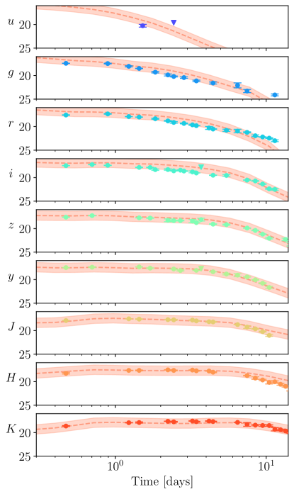
Figure 2: Best-fit light curve model from Bu2023Ye tight run on top of the AT2017gfo data. The data points are mostly within the 1mag systematics uncertainty band from the best-fit light curves, with $\chi^{2}/{\rm d.o.f.}=0.447$.

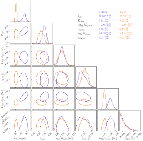
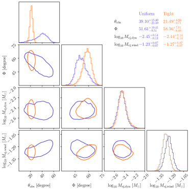
Figure 3: Comparison between the inference results for the Bu2023Ye (left) and the Bu2019lm (right) models with the inclusion of a tight Gaussian prior (orange) and a uniform inclination prior (blue). The median values (with $95\%$ credibility uncertainty) of parameters are also shown.

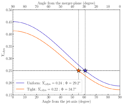
Figure 4: Constraints on the extension of the lanthanide-poor squeezed-polar ($Y_{\rm e,dyn}\geq 0.25$) and lanthanide-rich tidal-equatorial ($Y_{\rm e,dyn}<0.25$) dynamical ejecta for the Bu2023Ye model. The viewing angle dependence used in POSSIS (Eq. 2), together with the averaged values $\bar{Y}_{\rm e,dyn}=0.22\,(0.24)$ inferred from the uniform (tight) run suggests that the half-opening angle of the lanthanide-rich component is $\Phi=34.7^{\circ}$ ($29.2^{\circ}$).

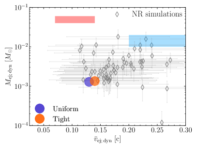
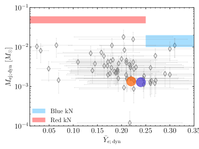
Figure 5: Predictions for the dynamical ejecta properties: mass, velocity, and electron fraction (as listed in Tab. 2) alongside the data from numerical-relativity simulations of BNS mergers (see text for details) and previous expectations for AT2017gfo from Siegel (2019) (shown as blue and red boxes for the two components of ejecta considered). Our measurements for the dynamical and wind ejecta masses and velocities (colored circles) are compared to numerical relativity simulations from Nedora et al. (2021a).

4 Discussion

Our results provide us with new insights into the angular distribution of ejecta composition of AT2017gfo. Our analysis of the light curve of AT2017gfo with the updated Bu2023Ye model with time-dependent opacities is more robust than previous studies relying on the Bu2019lm model. Here we first discuss how the inclusion of the inclination angle constraint modifies the geometry and the composition of the ejecta relative to a uniform inclination angle case.

Compared to Bu2023Ye uniform, the Bu2023Ye tight run also favors a slightly more extended (i.e., wider-angle) equatorial dynamical ejecta component. However, we find a smaller value of $\Phi$ ($34.7^{\circ}$) compared to Bu2019lm. Since $\Phi$ controls the opening angle of the tidal dynamical ejecta, our results point towards a wide-angle squeezed-polar component and a narrow-angle tidal-equatorial component to the dynamical ejecta. The inclination angle constraint further solidifies that the observer’s line-of-sight is pointed toward the squeezed polar dynamical ejecta, which contributes to the observed early blue light curve and affects the kilonova color evolution. As shown in Fig. 6, a good fraction ($\gtrsim 50$%) of the radiation escaping at early times ($\lesssim 2$ d) to an observer at $\theta_{\rm obs}\sim 28^{\circ}$ originates in the lanthanide-poor squeezed-polar component, which is able to explain the early blue emission in AT2017gfo (see Fig. 2) without the need of additional sources as suggested in the literature (e.g. Arcavi et al., 2017; Kasliwal et al., 2017; Arcavi, 2018; Metzger et al., 2018; Piro & Kollmeier, 2018). Alternatively, for a kilonova with identical geometry and composition to what we infer from this study to appear without an early blue component to its light curve, the viewing angle would have to be $\gtrsim 55$ deg. An AT2017gfo-like kilonova would likely exhibit a blue-to-red color evolution for most observer viewing angles.

In addition to the analysis of observational data to reveal the properties of the ejecta, ab-inito numerical-relativity simulations with advanced input physics can also be used to predict the properties of the ejecta and to link these properties to the BNS source parameters; however, for an accurate estimation of the ejecta electron fraction, sophisticated neutrino transport schemes are required. In Fig. 5, we show the mass, average velocity, and electron fraction of dynamical ejecta from a large sample of numerical-relativity simulations that included neutrino transport. The sample is based on the data collected in Nedora et al. (2021a) and corresponds to the M0RefSet combined with M0/M1Set there. In these simulations, both neutrino emission and absorption were included, albeit in a different manner. In simulations with M0 neutrino scheme, neutrinos were assumed to move radially, depositing only energy to the fluid, while in M1 scheme, neutrino motion was unconstrained, and both energy and momentum deposition was included. These simulations were collected from the following works: Radice et al. (2018); Sekiguchi et al. (2015, 2016); Vincent et al. (2020); Perego et al. (2019); Nedora et al. (2019); Bernuzzi et al. (2020); Nedora et al. (2021b). Square red and blue boxes in Fig. 5 correspond to the expectations derived from the analysis of multiwavelength data of AT2017gfo (e.g., Villar et al., 2017; Perego et al., 2017) compiled by Siegel (2019). Notably, these kilonova models were largely semi-analytical or one-dimensional. With a more sophisticated, anisotropic radiation transport model that takes into account ejecta composition and structure, we obtain properties of the dynamical ejecta that are more consistent with what numerical-relativity simulations suggest (see cyan and orange circles in the figure). Specifically, the inferred ejecta velocities and electron fractions are now closer to the average values obtained with numerical-relativity simulations. This highlights the importance of multi-dimensional radiative transfer simulations for kilonova modelling (see also Kawaguchi et al., 2018; Korobkin et al., 2021; Collins et al., 2023; Kedia et al., 2023; Shingles et al., 2023).

In addition to the agreement with respect to the ejecta mass, the ejecta velocity, and also the electron fraction, we also find large consistency between the half-opening angle of about $35^{\circ}$ and numerical-relativity predictions, e.g., employing the prediction of Nedora et al. (2021a) for $\Phi$ using the mean value of $q$ and $\tilde{\Lambda}$ of Dietrich et al. (2020), we find $\Phi\sim 32.7^{\circ}$, which is consistent with our prediction (Fig. 4).

The low inferred average electron fraction of $\bar{Y}_{\rm e,dyn}=0.22$ hints at the formation of heavier species in the KN ejecta. Our inferred $\bar{Y}_{\rm e,dyn}=0.22$ for the tight prior run reveals a dynamical ejecta composition that varies between $Y_{\rm e,dyn}=0.17$ and $Y_{\rm e,dyn}=0.41$. Based on the nuclear reaction network calculations from Lippuner & Roberts (2015) and Rosswog et al. (2018), an ejecta composition of $Y_{\rm e,dyn}\lesssim 0.20$ can well reproduce the solar $r$-process abundance pattern at $2^{\rm nd}$ peak and beyond. Thus, by inferring that the distribution of electron fractions extends down to $Y_{\rm e,dyn}=0.17$, our work insinuates that AT2017gfo likely produced $3^{\rm rd}$ peak elements consistent with the solar $r$-process abundance pattern.

Finally, we can also compare our results with a recent study of Sneppen et al. (2023), which suggested that the broad absorption feature observed in the optical spectra of AT2017gfo and attributed to strontium (Watson et al., 2019) is consistent with a kilonova that is highly spherical at early times. Namely, the pole-to-equator variation in the density and $Y_{\rm e,dyn}$ distribution is constrained to be small and shifted towards relatively high values needed to produce strontium. Our results indicate the opposite, suggesting that a strong pole-to-equator variation in $Y_{\rm e}$ and lanthanide-rich compositions close to the equator are required to reproduce the observed light curve evolution.

5 Conclusions

In this work, we use a tight inclination constraint for GW170817/AT2017gfo from recent VLBI observations (Mooley et al., 2022) and explore how this affects parameter inference on the ejecta, with a particular focus on the composition/chemical distribution within the dynamical ejecta component. We present a new grid of 1024 kilonova models computed with the three-dimensional Monte Carlo radiative transfer code POSSIS that depends on five parameters: the mass ($M_{\mathrm{ej,dyn}}$), averaged velocity ($\bar{v}_{\mathrm{ej,dyn}}$) and averaged electron fraction ($\bar{Y}_{\mathrm{{e,dyn}}}$) of the dynamical ejecta, and the mass ($M_{\mathrm{ej,wind}}$) and averaged velocity ($\bar{v}_{\mathrm{ej,wind}}$) of the post-merger disk-wind ejecta. Guided by numerical-relativity simulations, an angular dependence of both density and electron fraction is assumed for the dynamical ejecta. Employing this grid, we train a feed-forward NN that allows us to compute generic light curves to perform Bayesian parameter estimation. The main results can be summarized as follows:

• The best-fit model to AT2017gfo when adopting a tight prior on the inclination angle corresponds to $M_{\mathrm{ej,dyn}}=1.3\times 10^{-3}\,M_{\odot}$, $\bar{v}_{\mathrm{ej,dyn}}=0.14$c, $\bar{Y}_{\mathrm{{e,dyn}}}=0.22$, $M_{\mathrm{ej,wind}}=4.8\times 10^{-2}\,M_{\odot}$ and $\bar{v}_{\mathrm{ej,wind}}=0.03$c. Compared to a run with no constraints on the inclination angle, the inferred masses are higher and the averaged electron fraction lower.

• The inferred averaged electron fraction of $\bar{Y}_{\mathrm{{e,dyn}}}=0.22$ points to a strong angular variation of composition within the dynamical ejecta, with the electron fraction varying from $Y_{\rm e,dyn}\sim 0.17$ in the merger plane to $Y_{\rm e,dyn}\sim 0.41$ at the pole. The lanthanide-rich ($Y_{\rm e}\lesssim 0.25$), tidal component is distributed around the merger plane with a half-opening angle $\Phi=35^{\circ}$, while the rest of the dynamical ejecta is lanthanide-poor ($Y_{\rm e}\gtrsim 0.25$).

• The viewing angle of GW170817/AT2017gfo is pointed towards the lanthanide-poor (blue), squeezed polar dynamical ejecta, which can explain the early light curves of the observed kilonova without the need for additional powering sources.

• The properties inferred for the dynamical ejecta are in good agreement with those predicted by numerical-relativity simulations, alleviating the tension found previously when adopting one-dimensional and/or semi-analytical kilonova models (see e.g. Siegel, 2019, for a review).

• The large extent of a lanthanide-rich component within the dynamical ejecta is in contrast with a recent claim, based on the analysis of the strontium P Cygni spectral feature in AT2017gfo, of a spherical kilonova and a small pole-to-equator variation of $Y_{\rm e}$ (Sneppen et al., 2023).

• The range of electron fraction values inferred for the dynamical ejecta, going as low as $Y_{\rm e,dyn}\sim 0.17$, leads to the production of $r-$process nuclei up to the $3^{\rm rd}$ $r-$process peak (e.g. Lippuner & Roberts, 2015; Rosswog et al., 2018).

Our study highlights the importance of using tight inclination constraints and state-of-the-art multi-dimensional kilonova modeling for parameter inference of the ejecta properties. Furthermore, we underscore our ability to probe the nucleosynthesis of heavy elements using just the early-time kilonova photometry alone. Given the sensitivity of current ground-based gravitational-wave detectors to distant neutron star mergers, detailed spectroscopy of associated kilonova counterparts to gravitational-wave sources may not always be tenable. With a precise inclination angle measurement from an associated on-axis GRB or via other means, one can employ this methodology to infer the chemical distribution of any kilonova’s ejecta using well-sampled early light curve data. This approach, paired with spectroscopic studies of nearby KNe, can enable a better understanding of the nucleosynthetic yields from a population of kilonovae.

Data Availability

The datasets used and the software used for the analysis can be found at (https://github.com/nuclear-multimessenger-astronomy/nmma). The interpolation models can be found on Zenodo (https://doi.org/10.5281/zenodo.8039909). The raw data will be made public once the paper is accepted to the journal.

Appendix A Flux contribution from different ejecta components

Fig. 6 shows the contribution to the bolometric light curves of the squeezed-polar dynamical ($Y_{\rm e}\geq 0.25$, blue), the tidal dynamical ($Y_{\rm e}<0.25$, red) and the wind (grey) ejecta components. light curves refer to a dedicated ($N_{\rm ph}=10^{7}$) Bu2023Ye simulation made with POSSIS for the best-fit parameters of the tight run and for an observer viewing angle of $\theta_{\rm obs}=28^{\circ}$. At early times ($\lesssim 2$ d), a significant fraction ($\gtrsim 50$%) of the escaping radiation originates in the squeezed-polar lanthanide-poor component.

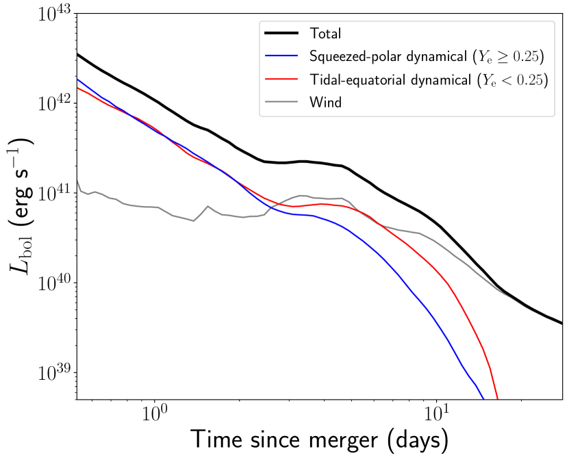
Figure 6: Contribution to the total bolometric light curve (black) of the squeezed-polar dynamical ($Y_{\rm e}\geq 0.25$, blue), tidal-equatorial dynamical ($Y_{\rm e}<0.25$, red) and wind (grey) ejecta components. light curves have been computed with a dedicated POSSIS simulation with $N_{\rm ph}=10^{7}$ using the best-fit parameters of the Bu2023Ye tight run and for an observer viewing angle of $\theta_{\rm obs}=28^{\circ}$.

References

- Abbott et al. (2017) Abbott B. P., et al., 2017, Phys. Rev. Lett., 119, 161101
- Almualla et al. (2021) Almualla M., Ning Y., Salehi P., Bulla M., Dietrich T., Coughlin M. W., Guessoum N., 2021, arXiv e-prints, p. arXiv:2112.15470
- Andreoni et al. (2017) Andreoni I., et al., 2017, Publ. Astron. Soc. Australia, 34, e069
- Arcavi (2018) Arcavi I., 2018, ApJ, 855, L23
- Arcavi et al. (2017) Arcavi I., et al., 2017, Nature, 551, 64
- Barnes et al. (2016) Barnes J., Kasen D., Wu M.-R., Martínez-Pinedo G., 2016, ApJ, 829, 110
- Bernuzzi et al. (2020) Bernuzzi S., et al., 2020, Mon. Not. Roy. Astron. Soc.
- Buchner et al. (2014) Buchner J., et al., 2014, Astron. Astrophys., 564, A125
- Bulla (2019) Bulla M., 2019, Monthly Notices of the Royal Astronomical Society, 489, 5037
- Bulla (2023) Bulla M., 2023, MNRAS, 520, 2558
- Chornock et al. (2017) Chornock R., et al., 2017, The Astrophysical Journal, 848, L19
- Collins et al. (2023) Collins C. E., Bauswein A., Sim S. A., Vijayan V., Martínez-Pinedo G., Just O., Shingles L. J., Kromer M., 2023, MNRAS, 521, 1858
- Coulter et al. (2017) Coulter D. A., et al., 2017, Science, 358, 1556
- Cowperthwaite et al. (2017) Cowperthwaite P. S., et al., 2017, ApJ, 848, L17
- Dietrich et al. (2020) Dietrich T., Coughlin M. W., Pang P. T. H., Bulla M., Heinzel J., Issa L., Tews I., Antier S., 2020, Science, 370, 1450
- Drout et al. (2017) Drout M. R., et al., 2017, Science, 358, 1570
- Evans et al. (2017) Evans P. A., et al., 2017, Science, 358, 1565
- Feroz et al. (2009) Feroz F., Hobson M. P., Bridges M., 2009, MNRAS, 398, 1601
- Fong et al. (2019) Fong W., et al., 2019, ApJ, 883, L1
- Fujibayashi et al. (2023) Fujibayashi S., Kiuchi K., Wanajo S., Kyutoku K., Sekiguchi Y., Shibata M., 2023, Astrophys. J., 942, 39
- Ghirlanda et al. (2019) Ghirlanda G., et al., 2019, Science, 363, 968
- Goldstein et al. (2017) Goldstein A., et al., 2017, The Astrophysical Journal, 848, L14
- Heinzel et al. (2021) Heinzel J., et al., 2021, Monthly Notices of the Royal Astronomical Society, 502, 3057
- Kasen et al. (2017) Kasen D., Metzger B., Barnes J., Quataert E., Ramirez-Ruiz E., 2017, Nature, 551, 80
- Kasliwal et al. (2017) Kasliwal M. M., et al., 2017, Science, 358, 1559
- Kasliwal et al. (2022) Kasliwal M. M., et al., 2022, MNRAS, 510, L7
- Kawaguchi et al. (2018) Kawaguchi K., Shibata M., Tanaka M., 2018, ApJ, 865, L21
- Kawaguchi et al. (2020) Kawaguchi K., Shibata M., Tanaka M., 2020, ApJ, 889, 171
- Kawaguchi et al. (2022) Kawaguchi K., Fujibayashi S., Hotokezaka K., Shibata M., Wanajo S., 2022, ApJ, 933, 22
- Kedia et al. (2023) Kedia A., et al., 2023, Physical Review Research, 5, 013168
- Kilpatrick et al. (2017) Kilpatrick C. D., et al., 2017, Science, 358, 1583
- Korobkin et al. (2021) Korobkin O., et al., 2021, ApJ, 910, 116
- Lamb et al. (2019) Lamb G. P., et al., 2019, ApJ, 870, L15
- Lee et al. (2017) Lee J., Bahri Y., Novak R., Schoenholz S. S., Pennington J., Sohl-Dickstein J., 2017, arXiv e-prints, p. arXiv:1711.00165
- Lippuner & Roberts (2015) Lippuner J., Roberts L. F., 2015, ApJ, 815, 82
- Lipunov et al. (2017) Lipunov V. M., et al., 2017, ApJ, 850, L1
- Lucy (1999) Lucy L. B., 1999, A&A, 344, 282
- Makhathini et al. (2021) Makhathini S., et al., 2021, ApJ, 922, 154
- Margutti et al. (2017) Margutti R., et al., 2017, ApJ, 848, L20
- Margutti et al. (2018) Margutti R., et al., 2018, ApJ, 856, L18
- McCully et al. (2017) McCully C., et al., 2017, ApJ, 848, L32
- Metzger (2019) Metzger B. D., 2019, Living Reviews in Relativity, 23, 1
- Metzger & Fernández (2014) Metzger B. D., Fernández R., 2014, MNRAS, 441, 3444
- Metzger et al. (2018) Metzger B. D., Thompson T. A., Quataert E., 2018, ApJ, 856, 101
- Mooley et al. (2018) Mooley K. P., et al., 2018, Nature, 561, 355
- Mooley et al. (2022) Mooley K. P., Anderson J., Lu W., 2022, Nature, 610, 273
- Nedora et al. (2019) Nedora V., Bernuzzi S., Radice D., Perego A., Endrizzi A., Ortiz N., 2019, Astrophys. J., 886, L30
- Nedora et al. (2021a) Nedora V., et al., 2021a, Classical and Quantum Gravity, 39, 015008
- Nedora et al. (2021b) Nedora V., et al., 2021b, ApJ, 906, 98
- Nicholl et al. (2017) Nicholl M., et al., 2017, ApJ, 848, L18
- Pang et al. (2022) Pang P. T. H., et al., 2022, arXiv e-prints, p. arXiv:2205.08513
- Perego et al. (2017) Perego A., Radice D., Bernuzzi S., 2017, Astrophys. J., 850, L37
- Perego et al. (2019) Perego A., Bernuzzi S., Radice D., 2019, Eur. Phys. J., A55, 124
- Pian et al. (2017) Pian E., et al., 2017, Nature, 551, 67
- Piro & Kollmeier (2018) Piro A. L., Kollmeier J. A., 2018, ApJ, 855, 103
- Pooley et al. (2018) Pooley D., Kumar P., Wheeler J. C., Grossan B., 2018, ApJ, 859, L23
- Radice et al. (2018) Radice D., Perego A., Hotokezaka K., Fromm S. A., Bernuzzi S., Roberts L. F., 2018, ApJ, 869, 130
- Rosswog & Korobkin (2022) Rosswog S., Korobkin O., 2022, arXiv e-prints, p. arXiv:2208.14026
- Rosswog et al. (2018) Rosswog S., Sollerman J., Feindt U., Goobar A., Korobkin O., Wollaeger R., Fremling C., Kasliwal M. M., 2018, A&A, 615, A132
- Savchenko et al. (2017) Savchenko V., et al., 2017, The Astrophysical Journal, 848, L15
- Sekiguchi et al. (2015) Sekiguchi Y., Kiuchi K., Kyutoku K., Shibata M., 2015, Phys.Rev., D91, 064059
- Sekiguchi et al. (2016) Sekiguchi Y., Kiuchi K., Kyutoku K., Shibata M., Taniguchi K., 2016, Phys. Rev., D93, 124046
- Setzer et al. (2023) Setzer C. N., Peiris H. V., Korobkin O., Rosswog S., 2023, MNRAS, 520, 2829
- Shappee et al. (2017) Shappee B. J., et al., 2017, Science, 358, 1574
- Shingles et al. (2023) Shingles L. J., et al., 2023, arXiv e-prints, p. arXiv:2306.17612
- Siegel (2019) Siegel D. M., 2019, Eur. Phys. J. A, 55, 203
- Smartt et al. (2017) Smartt S. J., et al., 2017, Nature, 551, 75
- Sneppen et al. (2023) Sneppen A., Watson D., Bauswein A., Just O., Kotak R., Nakar E., Poznanski D., Sim S., 2023, Nature, 614, 436
- Soares-Santos et al. (2017) Soares-Santos M., Holz D., Annis J., Chornock R., Herner K., 2017, Astrophys. J. Lett., 848, L16
- Tanaka et al. (2020) Tanaka M., Kato D., Gaigalas G., Kawaguchi K., 2020, MNRAS, 496, 1369
- Tanvir et al. (2017) Tanvir N. R., et al., 2017, ApJ, 848, L27
- Utsumi et al. (2017) Utsumi Y., et al., 2017, PASJ, 69, 101
- Valenti et al. (2017) Valenti S., et al., 2017, ApJ, 848, L24
- Villar et al. (2017) Villar V. A., et al., 2017, ApJ, 851, L21
- Vincent et al. (2020) Vincent T., Foucart F., Duez M. D., Haas R., Kidder L. E., Pfeiffer H. P., Scheel M. A., 2020, Phys. Rev., D101, 044053
- Watson et al. (2019) Watson D., et al., 2019, Nature, 574, 497
- Wollaeger et al. (2018) Wollaeger R. T., et al., 2018, MNRAS, 478, 3298
- Yu et al. (2018) Yu Y.-W., Liu L.-D., Dai Z.-G., 2018, ApJ, 861, 114