Machine learning Majorana nanowire disorder landscape

Abstract

We develop a practical machine learning approach to determine the disorder landscape of Majorana nanowires by using training of the conductance matrix and inverting the conductance data in order to obtain the disorder details in the system. The inversion carried out through machine learning using different disorder parametrizations turns out to be unique in the sense that any input tunnel conductance as a function of chemical potential and Zeeman energy can indeed be inverted to provide the correct disorder landscape. Our work opens up a qualitatively new direction of directly determining the topological invariant and the Majorana wave-function structure corresponding to a transport profile of a device using simulations that quantitatively match the specific conductance profile. In addition, this also opens up the possibility for optimizing Majorana systems by figuring out the (generally unknown) underlying disorder only through the conductance data. An accurate estimate of the applicable spin-orbit coupling in the system can also be obtained within the same scheme.

Introduction.— Hybrid superconductor-semiconductor (SC-SM) nanowire structures are the most extensively studied systems for creating laboratory Majorana zero modes (MZMs), which are localized non-Abelian excitations that can be used for creating a topological quantum computer. [3, 9, 20]. A recent experiment [3] has provided extensive tunnel conductance measurements to make the case for the existence of small and fragile topological regimes where MZMs should exist at the wire ends. Earlier experiments in such nanowires were strongly adversely affected by unintentional disorder in the system with the MZM-like conductance signatures arising from disorder-induced trivial Andreev bound states (and not from topological MZMs). [29, 9, 4, 28, 14, 21, 16, 15] Although cleaner samples are used in [3], the disorder situation even for this latest experiment is not yet completely clarified, but the small fragile gaps reported in [3] indicate that random disorder is likely still playing a role. [22, 23] Disorder has thus emerged as the single most important physical mechanism suppressing topology, certainly in Majorana nanowires, but likely in most solid state topological platforms. Although the possible importance of disorder in suppressing MZM physics was pointed out early [13, 12, 5, 11, 2, 6, 26, 7, 19, 18, 24, 25], we still do not have any direct information about the disorder in actual samples, hindering progress in the field. Understanding and controlling unintentional (and thus, unknown) random disorder has become by far the most important problem in the search for MZMs in solid state platforms. [9] Progress toward the realization of topological MZMs necessitates an understanding of the underlying disorder leading to cleaner and better samples. [[9, 22, 23]. This leads to the other key problem in the field of identifying MZMs in a device based on its transport characterization. This is because, as already mentioned, the unknown disorder leads to transport signatures that are often misinterpreted as MZMs, which often exist in a very limited part of parameter space in moderately disordered devices [2, 23]. Ultimately, this motivates the other key challenge in the field, which is to identify when an SC-SM nanowire device has been tuned to support MZMs.

In the current work, we introduce an intuitively appealing Machine Learning (ML) approach for figuring out and understanding the disorder landscape in Majorana nanowires using the tunnel conductance data, which are the standard measurements for Majorana nanowires carried out in every experiment (and simulated in the corresponding theories). The disorder potential together with other parameters can then be used to quantitatively verify the validity of the model, which in turn can be used to determine if the transport signature indicates a topological superconducting device. The idea is deceptively simple: The tunnel conductance depends crucially on disorder, and therefore, it should be possible to invert the measured conductance to extract the underlying disorder. Of course, the uniqueness of such an inverse scattering problem is a key question since, in principle, it is possible for different disorder landscapes to give similar conductance data. We solve the uniqueness problem a posteriori by showing that input disorder producing the conductance agrees with the output disorder obtained from our ML procedure. Our ML approach is powerful, and can be used to obtain other quantities entering the MZM physics, and we estimate the applicable spin-orbit coupling (a key parameter directly determining the nanowire topological gap) using our theory. As a matter of principle, the approach we use can be extended to improve estimates of other parameters of the model. The transport profile of such a complete model can be used to verify the model and provide the most direct correspondence so far of whether the specific transport profile corresponds to a topological device. We mention that other types of ML approaches have been used for optimizing gate operations in Majorana nanowires [27], but our work is totally different since we use ML to solve the inverse scattering problem of extracting the disorder by using tunnel conductance itself as our training data. More significantly, our ML approach, by providing the unknown parameters for the system, enables a direct realistic estimate for the topological invariant as a function of system parameters to decisively ascertain where the system is topological with MZMs and where it is trivial with no topological properties. This eliminates all subjective judgments about the topological nature of the system as ML itself provides an answer provided sufficient data are used for the training.

Theory.— We use the extensively used minimal 1D model for Majorana nanowires where the system Hamiltonian is given by a 1D BdG equation and the minimal input parameters are the effective mass (m), the spin-orbit coupling ($\alpha$), the Lande g-factor (g), the parent SC gap, the SC-SM coupling, the self-consistent chemical potential $\mu$, the magnetic field B, and the disorder potential $V_{\text{dis}}(x)$. We follow Ref. [23] where the details (which are standard in the literature to study SC-SM Majorana nanowires [20, 16]) can be found. Note that all quantities other than $V_{\text{dis}}$ and $\alpha$ are taken to be fixed and known although this constraint can be relaxed in future works (at the cost of needing much more data for training since more unknown parameters there are, larger must be the training data set). We use, following Ref. [3], a 3 micron long wire for all our results and discretize the BdG equation using a lattice size of 10 nm as in Ref. [23]. We provide the details for the theory and the model in the Supplementary Information (S-1 in SI).

Among these SC-SM nanowire parameters, the specific spatial dependence of the disorder potential $V_{\text{dis}}(x)$ is completely uncontrolled and varies among devices as well as slowly over time in the same device. In addition, some system parameters such as $\alpha$ depend on the inversion symmetry breaking of the final device structure, which in general is unknown (and most likely varies from device to device). Given a $V_{\text{dis}}(x)$, we can solve the BdG equation and generate the 4-component tunnel conductance matrix using the KWANT scattering matrix approach. [10] In addition, we use the spin-orbit (SO) coupling $\alpha$ also as an unknown parameter. We vary the disorder potential and $\alpha$ to generate, using KWANT, training transport data (i.e. the 4-component conductance matrix G as a function of the magnetic field $B$ and the chemical potential $\mu$) set for our ML algorithm. We provide details of how the conductance matrix $G$ is computed as a function of $B,\mu$ and other parameters in S-1 of SI. The ML algorithm then predicts $V_{\text{dis}}$ and $\alpha$ that can be used using KWANT to reproduce a test transport data set. Ideally, in the test transport data would come from experiments. In our proof of principle demonstration, our test transport data is generated using KWANT with a random choice of $V_{\text{dis}}(x)$ and $\alpha$. The real test of our ML success is whether the conductance generated using the output $V_{\text{dis}}(x)$ and $\alpha$ is close to the test transport data set.

Method.— Our machine learning model consists of a recurrent neural network (RNN) created by the package Keras [8] which builds upon tensorflow [1]. In our specific RNN (Fig. 1) each input step consists of a measurement operation, 7 parameters consisting of a row of X (4 parameters), which are the components of the conductance matrix $G_{\alpha\beta=L,R}$ and of K (3 parameters), which are the parameters bias voltage $V_{bias}$, chemical potential $\mu$ and magnetic field $B$. The 5 Fourier components of $V_{dis}(x)$ and $\alpha$ are organized into the output vector $Y$ of the RNN in Fig. 1. As described in S-1 of SI, the conductance matrix $X$ is generated for each instance of $K$ and $Y$ using a KWANT simulation. Later we will also discuss data where we use a $10$ Fourier component model for the disorder. In this case $Y$ would be a 11 component vector. For the purpose of ML, it is useful to organize the measurement data into a combined measurement result matrix $m=[X,K]$. The RNN is used so that the addition of more measurements would not decrease the ability of the previous measurements to perform predictions for a fixed amount of training data. We note that while our RNN is sufficient to provide a proof of principle, but can certainly be enhanced/expanded in the future by using more elaborate convolutional neural networks, as needed. In particular the RNN for the case of 5 disorder components contains 3 GRU hidden recurrent layers with 150 nodes each, which are then followed up with a non-recurrent 100 node dense hidden layer. For the 10 component model we instead use 5 GRU layers, still with 150 nodes each. (More ML technical details are given in S-II in SI.)

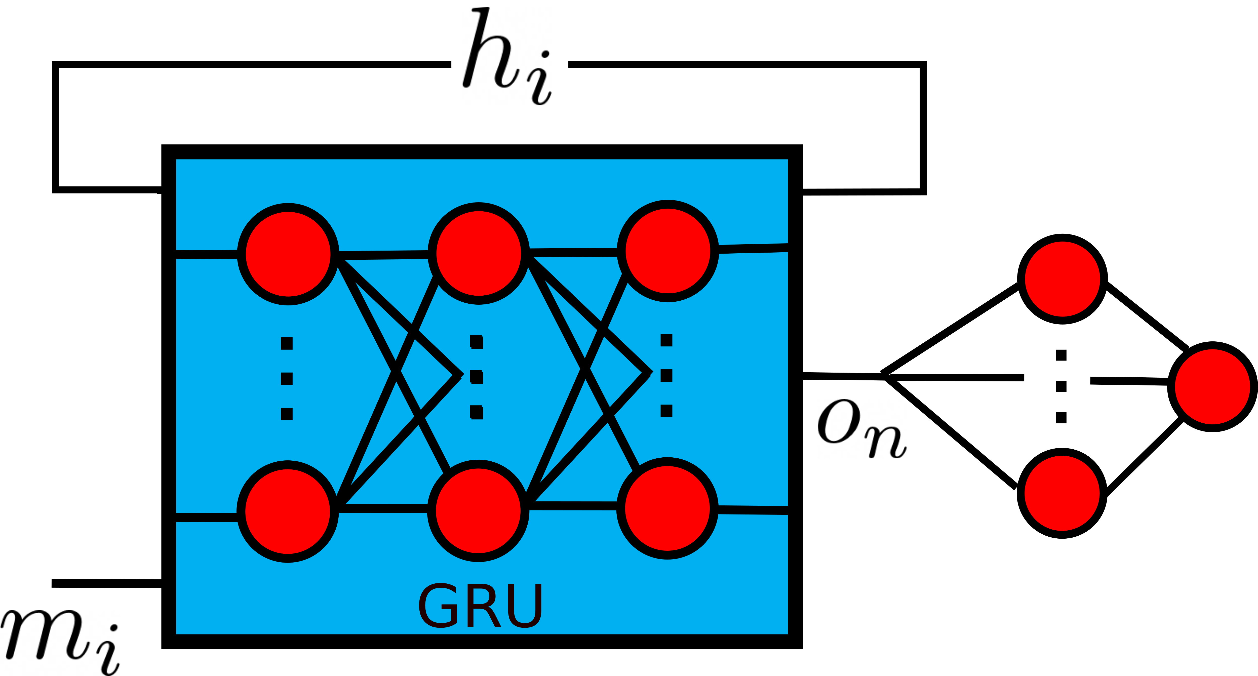
(a)

Figure 1: (a) Diagram of the neural network. The machine learning model consists of a recurrent neural network (RNN) portion followed by a dense layer. The RNN for the 5+1 (10) component model consisted 3 (5) GRU hidden recurrent layers with 150 nodes each, followed by a dense hidden layer with 100 nodes. $m_{i}$ is the $i^{\text{th}}$ row of m, $o_{n}$ is the final GRU output after $n$ iterations, where $n$ is the total number of rows within m. $h_{i}$ is the state vector after $i$ iterations of GRU. For the 5+1 component model the final output $Y$ contains $\alpha$ while for the 10 component model it’s just the Fourier components of disorder.

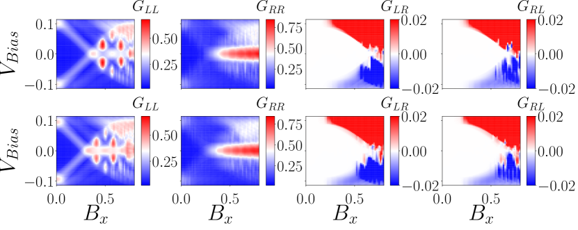
(a)

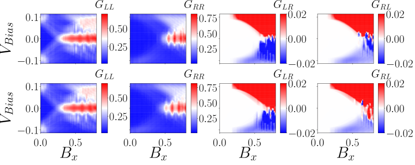
(b)

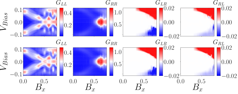
(c)

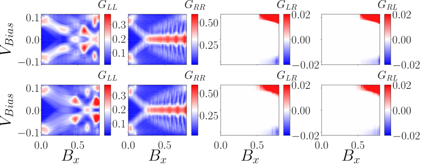
(d)

Figure 2: Representative samples of 5 disorder potential components and $\alpha$ neural network test input and predictions. In (a-d) the first row is $G_{LL}$, $G_{RR}$, $G_{LR}$ and $G_{RL}$ conductance simulations expected for the input disorder potential, and the second row is the calculated conductance measurements for the corresponding predicted disorder potential. Each of (a-d) is for different disorder potential and $\alpha$ realizations (shown in Fig.3). The topological invariant corresponding to this profile can be seen in Fig S4. The conductance simulations are plotted for different values of $V_{\text{Bias}}$ (in meV) and $B_{x}$ (in T). These are plotted for $\mu=0$

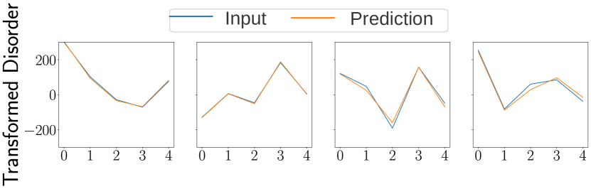
(a)

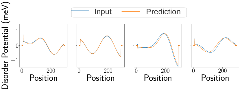
(b)

Figure 3: Representative samples of 5 disorder potential components neural network test input and predictions. (a) The discrete cosine transformed components of the disorder potential for 4 different samples and their respective predictions. (b) Disorder potentials in real space with deterministic modification due to boundary effects. The topological invariant corresponding to this profile can be seen in Fig S4. The disorder amplitude and correlation length for each realization was 1.5meV and 3 sites respectively. Input and output are virtually indistinguishable demonstrating the efficacy of the ML.

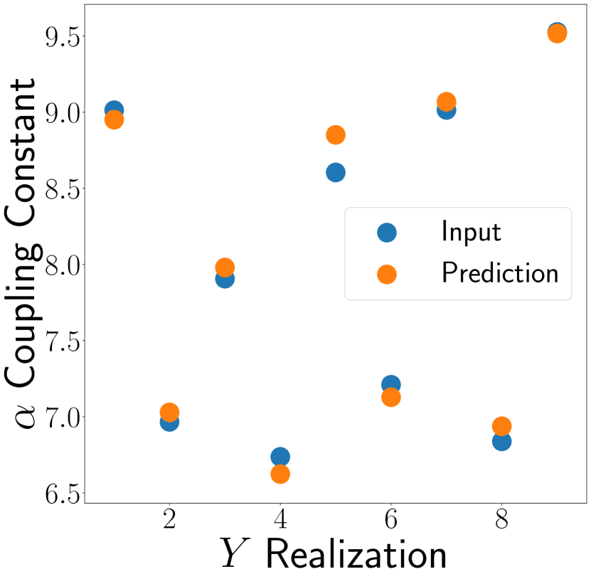
(a)

Figure 4: Representative samples of $\alpha$ neural network test input and predictions. The blue points representing the input $\alpha$ values (in meV/nm) and the orange represent the predicted $\alpha$ values.

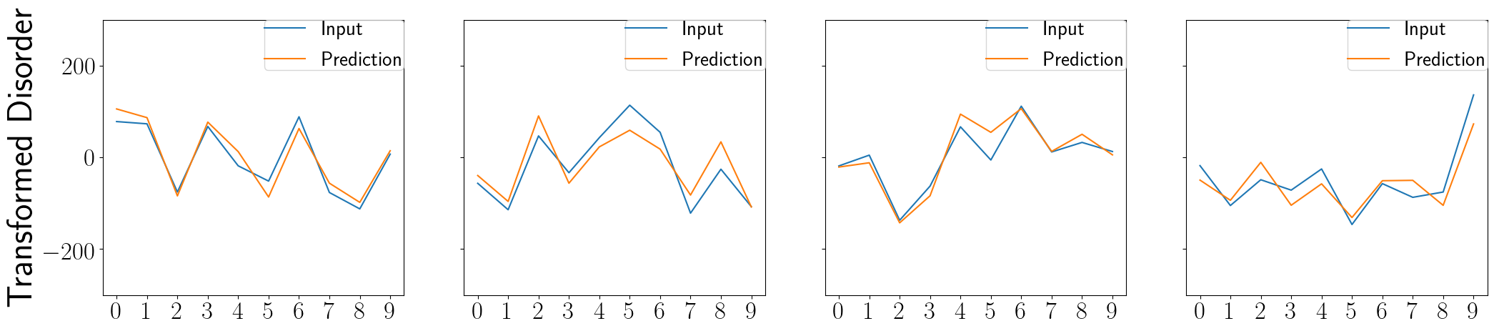
(a)

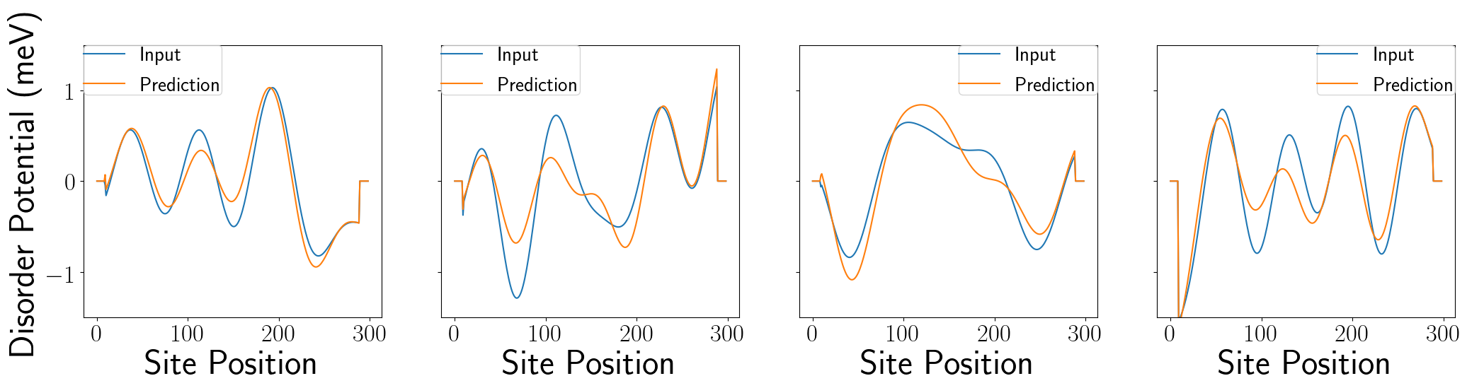
(b)

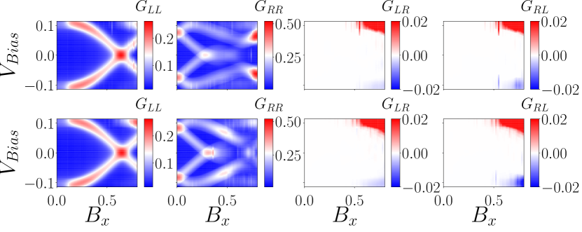
(c)

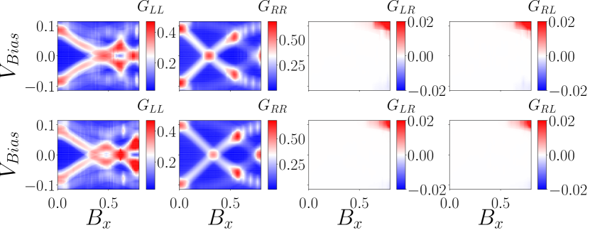
(d)

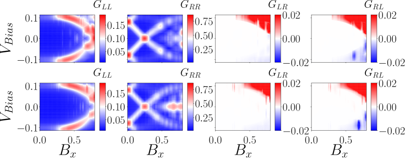
(e)

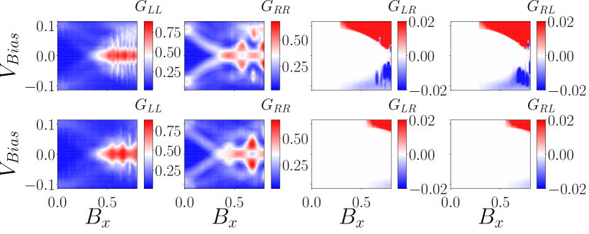
(f)

Figure 5: Representative samples of 10 disorder potential components neural network test input and predictions. (a) The discrete cosine transformed components of the disorder potential for 4 different samples and their respective predictions. (b) Disorder potentials in real space with deterministic modification due to boundary effects. Representative samples of 10 disorder potential components neural network test input and predictions. In (c-f) the first row is $G_{LL}$, $G_{RR}$, $G_{LR}$ and $G_{RL}$ conductance measurements expected from a input disorder potential, and the second row is conductance measurements from the corresponding predicted disorder potential. Each of (c-f) are different disorder potential realizations, shown in (a). The conductance measurements are plotted for different values of $V_{\text{Bias}}$ (in meV) and $B_{x}$ (in T). For this model $\alpha=8meV/nm$ is fixed. The topological invariant corresponding to this profile can be seen in Fig S5. The disorder amplitude and correlation length for each realization was $1.5$meV and 3 sites respectively. These are plotted for $\mu=0$.

Results.— We use both 5-component and 10-component representations for our Gaussian random disorder, obtaining very similar results. We measure the ML effectiveness using the standard scaled $R_{2}$ fidelity parameter between the $Y_{test}$ and $Y_{predicted}$ predicted by the trained RNN. The standard scaling converts the data used in the training processes into a zero mean, unit variance form. $R_{2}=1$ implies perfect prediction, while $R_{2}=0$ is equivalent to just taking the average output of the testing data, ie., no prediction. This scaling and $R_{2}$ can be found in details on the package scikit-learn [17].

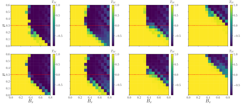
(a)

Figure S4: Representative samples of the topological invariant ($T_{IV}$) for 5 disorder potential components and $\alpha$ neural network test input and predictions. The first row is $T_{IV}$ resulting from a input disorder potential, and the second row is from the corresponding predicted disorder potential. Each column are the different disorder potential realizations, shown in Fig.3. The dotted red line corresponds to the conductance profiles in Fig. 2. The topological invariant is plotted for different values of $\mu$ (in meV) and $B_{x}$ (in T).

To train the model for 5 disorder components we generate a total of 8000 $Y$ realizations for a fixed disorder strength. We split our data such that 90% is used in the training process and the remaining 10% used for testing. Using the 800 test realizations we achieve a standard scaled $R_{2}$ = 0.98, which is an excellent fidelity. For this model we find it sufficient to use only the zero bias conductance data (i.e. set $V_{bias}=0$ in $K$) to obtain the $98\%$ fidelity already. We emphasize that the ML algorithm predicts $V_{\text{dis}}$, $\alpha$ accurately enough that they predicted values can be used in KWANT to match a test conductance quite accurately as seen in Fig. 2. The good $R_{2}$ value of the predictions of the RNN are apparent from comparing the test and predicted Fourier components of disorder and SO coupling seen in Figs. 3 and  4. (More results are given in the S-III in the SI.) The accuracy of the predicted parameters implies that the $Y$ values predicted by the RNN can also be used to generate the topological invariant in parameter (i.e. $K$) space. To test this we compared the topological visibility in $B-\mu$ space between a test case and predicted case and found good agreement as seen in Figs. S4 S5 S6 in the SI.

In Fig. 5, we show the results of our 10-component disorder ML results. To train for 10 disorder components we generate a total of 20000 disorder realizations, 90% of which is used in the training process and the remaining 10% used to test. We use a fixed $\alpha=8.0meV/nm$. Using the 2000 test realizations we achieve a standard scaled $R_{2}=0.79$, which is respectable, but can be improved with more data sets. Due to computational limitations we only use $V_{\text{Bias}}=0$ and $V_{\text{Bias}}=0.032$ meV (using more values of $V_{\text{Bias}}$ should increase $R_{2}$). This lower fidelity is likely due to the need for more training and a larger $K$ matrix since differentiating among 10 component potentials is a more computationally challenging task. Representative results are shown in Fig. 5, and again, visual inspection shows excellent agreement between the input/output data, verifying the success of our ML approach.

Conclusion.—We introduce a Machine Learning approach to extract unknown system parameters, particularly the disorder landscape, from the simulated (or measured) tunnel conductance data in hybrid SC-SM Majorana nanowire structures. We validate the approach by using simulated conductance data as the training set, establishing that such training leads to strongly predictive results for both disorder and spin-orbit coupling using as few as 3 parameters (i.e. $K$) for the conductance data used in our simulations. The accuracy of the predicted results can be verified by comparing the predicted conductance as well as topological visibility profiles to the test profiles. The predicted profiles, which are functions of multiple parameters such as $V_{bias}$ and $\mu$ are generated by KWANT from the parameters that are predicted by ML to match a given test conductance data. The topological visibility profile as a function of $B$ and $\mu$ is also generated by KWANT for test conductance data generated by KWANT. Using experimental conductance data (and a bigger computer), one should be able to generalize our approach to obtain all the relevant parameters for Majorana nanowires, not only the disorder and the SO coupling as we do, but also the g-factor, the SC gap, the number of occupied subbands, etc. since our ML approach is general, and only requires as inputs sufficient amount of conductance training data which are easy to obtain both experimentally and theoretically. Our method, given enough training data and computing resources, should in principle be able to decisively indicate, just through our ML protocol, whether a set of conductance data in a particular sample indicates an underlying topological (or trivial) system with MZMs (or not). In particular, by determining all the relevant unknowns, one can simulate a device and calculate its topological invariant directly using the output parameters, decisively indicating whether the sample is or is not topological.

I Acknowledgement

We thank Maissam Barkeshli for teaching a machine learning course which helped us in developing our approach presented in this paper. This work is supported by the Laboratory for Physical Sciences.

Supplemental Materials: Machine learning Majorana nanowire disorder landscape

S-I Details of theory

We model the 1D semiconductor Majorana nanowire using a Bogoliubov-de Gennes Hamiltonian [6]:

$$H=\left(-\frac{\hbar^{2}}{2m^{*}}\partial_{x}^{2}-i\alpha\partial_{x}\sigma_{y}-\mu+V_{\text{dis}}(x)\right)\tau_{z}\\ +\frac{1}{2}g\mu_{B}B\left(\sigma_{x}\cos\theta+\sigma_{y}\sin\theta\right)+\Sigma(\omega)$$ (S1)

where

$$\Sigma(\omega)=-\gamma\frac{\omega+\Delta_{0}\tau_{x}}{\sqrt{\Delta_{0}^{2}-\omega^{2}}}$$

is the self-energy generated by integrating out the superconductor that is proximity coupled to the semiconductor [11]. The above Hamiltonian is a $4\times 4$ matrix comprised of $\sigma_{x,y,z}$, which are $2\times 2$ Pauli matrices associated with the spin degree of freedom, and $\tau_{x,y,z}$, which are $2\times 2$ Pauli matrices associated with the superconducting particle-hole degree of freedom. The above Hamiltonian is written in a basis where the Bogoliubov quasiparticles of the superconductor are described by a Nambu spinor with a structure $\psi(x)=(u_{\uparrow}(x),u_{\downarrow}(x),-v_{\downarrow}(x),v_{\uparrow}(x))^{T}$, where $\uparrow,\downarrow$ refer to spin and $u,v$ refer to particle-hole components of the quasiparticle. The frequency $\omega$ in the self-energy is equivalent to the energy (in units where $\hbar=1$) of the Bogoliubov quasiparticle in consideration. While, this requires a self-consistent solution for eigenstates in a closed system, the $\omega$ dependence of $\Sigma$ does not present any additional complication in the solution of transport problems in open systems using KWANT [5]. Specifically, KWANT solves the transport problem of the Majorana nanowire by computing the scattering matrix of the system in the particle-hole space between the two leads shown in Fig. S1. The scattering matrix can be used to compute the conductance matrix $G_{\alpha\beta}$ using the well-known Blonders-Tinkham-Klapwijk relations [5]. In addition, one can use the reflection matrix from either of the lead ends to compute the topological visibility $T_{IV}$ [3, 8].

The actual semiconductor device is a complicated three dimensional semiconductor system. Despite this, the transport properties computed by KWANT [5] using the model Hamiltonian Eq. S1 captures most qualitative features of the transport properties of the device over the relevant ranges of gate and bias voltages provided the parameters $\alpha$, $\mu$ etc are taken to be fitting parameters. Therefore, the parameters $m^{*}$, $\alpha$, $\ldots$ should ideally be viewed as fitting parameters to transport properties of devices. In practice [8, 12, 10], the parameters such as effective mass $m^{*}=0.03m_{e}$ and a nominal (details later) value of the spin-orbit coupling $\alpha=8.0\,meV-nm$ are chosen to fit non-superconducting transport characterization of the InAs nanowire device. The superconducting pairing potential coupling parameter $\gamma=0.15\,meV$, the Lande g-factor $g=25$ are chosen to qualitatively reproduce transport properties in the superconducting phase. The intrinsic superconducting pair potential $\Delta_{0}=0.12\,meV$ is chosen according to be the superconducting gap of the Al superconductor. In addition, to model transport in the system given by the Hamiltonian in Eq. S1, we choose a temperature $T=50mK$, and device length $L=3\,\mu m$. The finite temperature is implemented in the system by convolving the zero temperature conductance as a function of $\omega$ with the derivative of a Fermi function at temperature $T$. For this purpose, we generate the zero-temperature conductance using KWANT at an $\omega$ grid with 151 points between $\pm 0.04$ meV. Finally, for the purpose of numerical simulations we discretize the Hamiltonian in Eq. S1 with a lattice scale of a=10 nm. These parameters are chosen from recent work [10], which was focused on understanding the recent experiments from the Microsoft group [2].

The disorder potential generated by impurities in the device is also included in the Hamiltonian $H$ through the function $V_{\text{dis}}(x)$. The spatial disorder potential is assumed to randomly varying with position $x$ across the length of the wire with a Gaussian distribution with an amplitude $1.5\,\text{meV}$ and correlation length of $30\,nm$. For the purposes of simplifying the ML complexity by reducing the number of parameters, we eliminate (i.e. set to 0) all but $N_{dis}$ of the Fourier components of the disorder potential. For our calculations we will use $N_{dis}=5$ or $10$. In addition, we also include barrier potentials $V_{\text{Barrier}}^{L}$ and $V_{\text{Barrier}}^{R}$ as $\delta$ function contributions at the ends of the wire to $V_{\text{dis}}(x)$.

Out of the parameters that go into $H$, the spacial profile of the disorder potential $V_{\text{dis}}(x)$, which is specified in our model by the $N_{dis}$ Fourier components, is completely uncontrolled and varies between devices as well as slowly over time. In addition, some parameters such as $\alpha$ depend on the inversion symmetry breaking of the final device structure, where it is difficult to interpret the transport data. In this work, we will vary the disorder potential and spin-orbit coupling $\alpha$ (around the aforementioned nominal value) to generate, using KWANT, training transport data set as a function of chemical potential $\mu$, magnetic field $B$ and bias voltage $V_{bias}$ (related to $\omega$ in $H$) to be fit by an ML algorithm. To keep the computation in this work simple, we assume the other parameters in the Hamiltonian $H$ are fixed at values estimated from experiment. The ML algorithm will then predict the Fourier components of $V_{\text{dis}}$ and spin-orbit coupling $\alpha$ from transport that can be used using KWANT to match a test transport data. Ideally, the test transport data would come from experiment though that would likely require more fit parameters. In our proof of principle demonstration, our test transport data is generated using KWANT using a random choice of disorder configuration and $\alpha$.

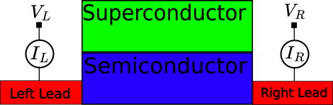
(a)

Figure S1: Sketch of Majorana nanowire device. The device consists of a NS junction with a layer of superconductor on top of a layer of semiconductor, with opposite ends of the semiconductor connected to left and right leads respectively [7]. The differential conductances, which are measured, are defined as $G_{\alpha\beta}=dI_{\alpha}/dV_{\beta}$ for $\alpha=\beta$ and $G_{\alpha\beta}=-dI_{\alpha}/dV_{\beta}$ for $\alpha\neq\beta$. Local conductances $G_{LL}$ and $G_{RR}$ are measured from their respective leads through the junction (to the superconductor), while non-local conductances $G_{RL}$ and $G_{LR}$ are measured from the right lead to the left lead or the reverse respectively.

S-II Details of Machine Learning

S-II.1 Training Data

The training data was generated within KWANT for many different randomly generated $V_{\text{dis}}(x)$ and $\alpha$ configurations (called Y realizations). For each Y realization we calculate a set of $G_{\text{RR}}$, $G_{\text{LL}}$, $G_{\text{RL}}$, $G_{\text{LR}}$ values for different measurement configurations. A Y realization consists of generating a random $\alpha$ from a uniform distribution between 6.4 and 9.6, along with a random Gaussian disorder potential. The disorder potential $V_{\text{dis}}(x)$ refers to disorder within the $\mu$ chemical energy taking $\mu\rightarrow\mu+V_{dis}(x)$. The disorder potential is transformed with a discrete cosine transform, and only the nth lowest frequency components are kept. This gives us $c_{1}...c_{n}$, the transformed disorder potential components. The transformation is then undone to get the disorder potential in real space corresponding to these components. This truncated then reverse transformed $V_{dis}(x)$ is what will be used by KWANT. From the transformed components we define a vector for each Y realization:

$$Y=\begin{bmatrix}c_{1}&\ldots&c_{n}&\alpha\end{bmatrix}$$

This is done for many different Y realizations, each time having the potential along with $\alpha$ numerically simulated to evaluate a sequence of conductance measurements. The measurement configurations were recorded in a matrix $K$ where each row would record a particular setup of experimentally tunable parameters labelled as j:

$$\textbf{K}_{\text{full}}=\begin{bmatrix}\mu^{j}&B^{j}&V^{L,j}_{\text{Barrier}}&V^{R,j}_{\text{Barrier}}&\theta^{j}&V^{j}_{\text{Bias}}\end{bmatrix}$$

where $B$ is the applied magnetic field, $\mu$ is the chemical potential parameter controlled by the plunger gate voltage, $V^{L}_{\text{Barrier}}$ and $V^{R}_{\text{Barrier}}$ are the left and right barrier voltages respectively, $\theta$ is the angle of the B field relative to the direction of the wire, and $V_{\text{Bias}}$ is the bias voltage. All these are parameters that are readily varied in a transport experiment. The Hamiltonian that is described in the previous section, which is used in the KWANT simulation contains all of these parameters except $\theta$, which has been assumed to be zero for simplicity. The possibility of varying all these parameters to study transport provides the potential of generating a huge volume of transport data to characterize a specific device. In our case, we found it either unnecessary or beyond our limited computational resources to use transport data in the entire space to estimate the disorder in the device. As such we fixed $V^{L}_{\text{Barrier}}=V^{R}_{\text{Barrier}}=15$ meV and $\theta=0$. The simplified $\mathbf{K}$ we use is as follows:

$$\textbf{K}=\begin{bmatrix}\mu^{j}&B^{j}&V^{j}_{\text{Bias}}\end{bmatrix}$$

Furthermore, $V_{\text{Bias}}$ turns out to not be necessary to fit the transport data when 5 disorder Fourier components are used. Therefore, in this case it is removed from the $K$ matrix and set to $V_{\text{Bias}}=0$. In contrast, the 10 Fourier component disorder models require more transport data to fit and in this case we include $V_{\text{Bias}}$ in the $K$ matrix. For these calculations, $V_{\text{Bias}}$ takes one of two values $V_{\text{Bias}}=0$ meV and $V_{\text{Bias}}=32\,\mu eV$ depending on the realization index $j$. Each row of K when fed into KWANT generates a new set of conductance measurements, we put these conductances into a matrix we call X as follows:

$$\textbf{X}=\begin{bmatrix}G_{\text{RR}}^{j}&G_{\text{LL}}^{j}&G_{\text{RL}}^{j}&G_{\text{LR}}^{j}\end{bmatrix}$$

Putting this all together we get our training data generating function as follows:

$$F_{\text{Gen}}(Y;\textbf{K})=\textbf{X}$$

Note that all the different Y realizations have the same K matrix. It can be seen then that our objective is to find a function that can take in X and K, and give us $Y$. Put another way we wish to invert our generator function to find the following:

$$F^{-1}_{ML}(\textbf{X};K)=Y$$

In terms of the other components, we varied $\mu$ between 0 meV and 0.6 meV (with 15 steps), $B_{x}$ between 0 T and 0.8 T (with 15 steps). Overall our K matrix had 225*$N_{V_{\text{Bias}}}$ rows, as we do not feed all the $V_{\text{bias}}$ data into the neural network. $N_{V_{\text{Bias}}}=1$ and $N_{V_{\text{Bias}}}=2$ for 5 and 10 component versions respectively.

In summary we generate many random realizations of $V^{i}_{\text{dis}}(x)$ and $\alpha^{i}$, cosine transform each $V^{i}_{\text{dis}}(x)$ and truncate to either 5 or 10 components to form a $Y^{i}_{\text{input}}$. Using this we calculate $F_{\text{Gen}}(Y^{i}_{\text{input}};K)=X^{i}_{\text{input}}$, where within KWANT $Y^{i}_{\text{input}}$ is inverse cosine transformed back into real space. The $X_{\text{input}}^{i}$, $Y^{i}_{\text{input}}$ pairs are split between training $X_{\text{train}}^{i}$, $Y^{i}_{\text{train}}$ and testing $X_{\text{test}}^{i}$, $Y^{i}_{\text{test}}$. Using $X_{\text{train}}^{i}$, $Y^{i}_{\text{train}}$ we train a neural network to be able to generate a prediction for $Y$ given an $\mathbf{X}$. We assess the validity of our model by comparing $Y^{i}_{\text{test}}$ to our neural network prediction $F_{ML}^{-1}(\mathbf{X}_{\text{test}}^{i};K)=Y^{i}_{\text{{Pred}}}$.

S-II.2 The Neural Network

Our machine learning model consisted of a recurrent neural network (RNN) created the package Keras [4] which is a package that builds upon tensorflow [1]. In the RNN each input step consisted of a measurement operation, 10 parameters consisting of a row of X (4 parameters) and of K (6 parameters). For this reason it is useful for us to define a combined measurement result matrix $\textbf{m}=[\textbf{X},\textbf{K}]$. A RNN was used so that the addition of more measurements would not decrease the ability of the previous measurements to perform predictions for a constant amount of training data. This is sub-optimal as RNNs are order dependent, while the order one performs the conductance measurements shouldn’t matter. Ideally a convolution neural network (CNN) would be preferable, however since our K and thus measurement order is the same for all input an easier RNN was sufficient. In particular the RNN for the 5 disorder components and 1 alpha (5+1 component model) consisted of 3 GRU hidden recurrent layers with 150 nodes each, which were then followed up with a non-recurrent 100 node dense hidden layer. In the case of the 10 components model we instead had 5 GRU layers, still with 150 nodes each. A figure of this can be seen in Fig. 1.

We measure the effectiveness of our model using the standard scaled $R_{2}$. This is calculated between $\{Y^{i}_{\text{{test}}}\}$ and $\{Y^{i}_{\text{{Pred}}}\}$. The standard scaling converts the data used in the training processes into a 0 mean, unit variance form. A $R_{2}=1$ implies perfectly predicting the tests, while $R_{2}=0$ is equivalent to just taking the average output of the testing data. This scaling and $R_{2}$ can be found within the package Scikit-learn [9].

S-III Additional results

This section presents additional plots of numerical results, including the conductance plots of $\mu$ vs. $B_{x}$ and $T_{IV}$ plots for both the input and prediction Y realizations. We include the conductance plots because the machine learning model utilizes $\mu$ vs. $B_{x}$ as its main input during the training process. The $T_{IV}$ plots demonstrate the ML model’s capability to predict $T_{IV}$ solely based on conductance measurements. Moreover, we provide the conductance and $T_{IV}$ results for a pristine sample, which readers may find useful for comparison.

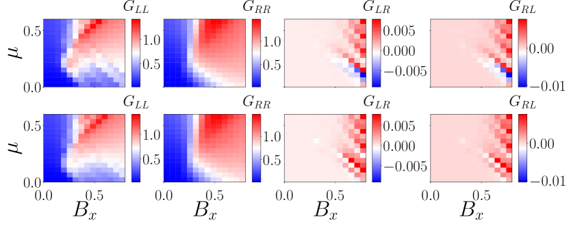
(a)

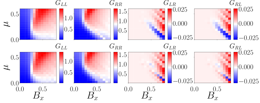
(b)

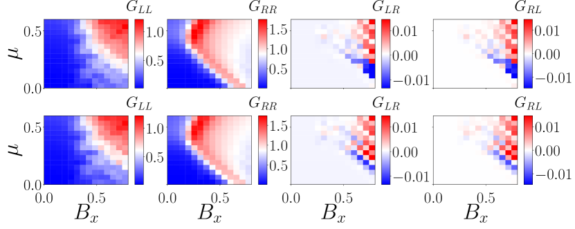
(c)

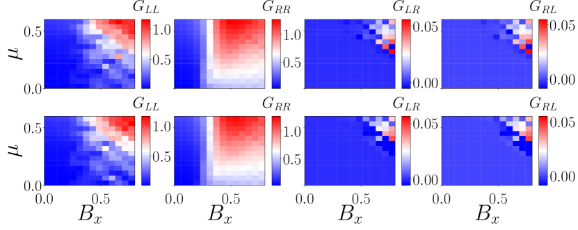
(d)

Figure S2: Representative samples of 5 disorder potential components and $\alpha$ neural network test input and predictions. In (a-d) the first row is $G_{LL}$, $G_{RR}$, $G_{LR}$ and $G_{RL}$ conductance measurements expected from a input disorder potential, and the second row is conductance measurements from the corresponding predicted disorder potential. Each of (a-d) is a different Y realization, shown in Fig.3. The conductance measurements are plotted for different values of $\mu$ (in meV) and $B_{x}$ (in T). The topological invariant corresponding to this profile can be seen in Fig S4. The disorder amplitude and correlation length for each realization was 1.5meV and 3 sites respectively. These plots use $V_{\text{Bias}}=0$.

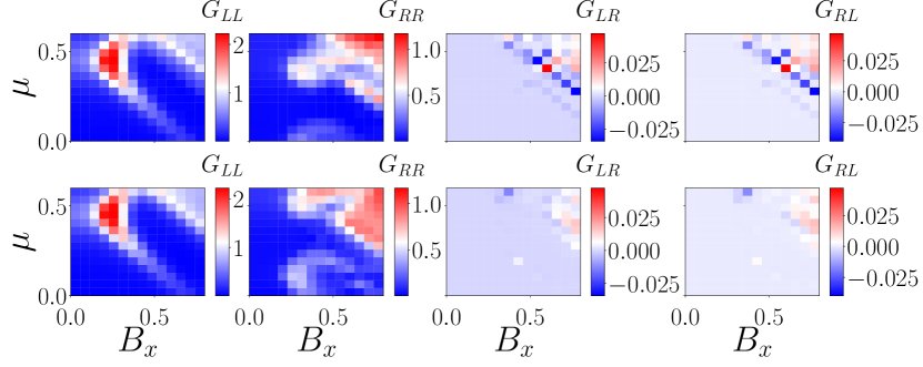
(a)

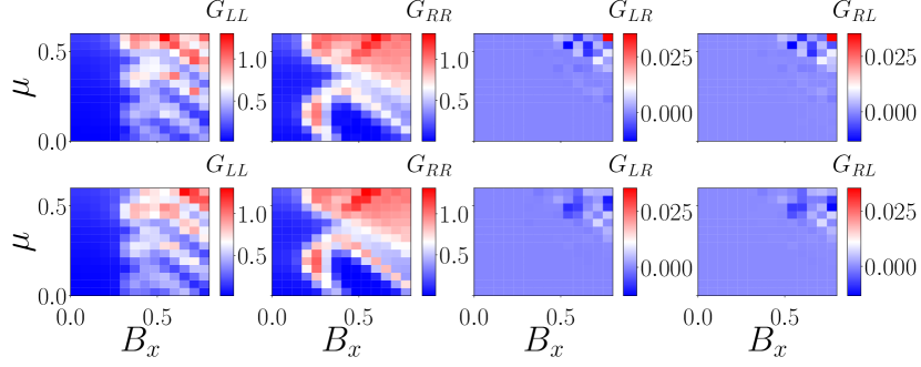
(b)

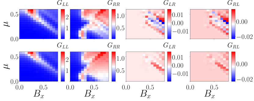
(c)

(d)

Figure S3: Representative samples of 10 disorder potential components neural network test input and predictions. In (a-d) the first row is $G_{LL}$, $G_{RR}$, $G_{LR}$ and $G_{RL}$ conductance measurements expected from a input disorder potential, and the second row is conductance measurements from the corresponding predicted disorder potential. Each of (a-d) are different disorder potential realizations, shown in Fig.5a. The conductance measurements are plotted for different values of $\mu$ (in meV) and $B_{x}$ (in T). For this model $\alpha=8\text{meV/nm}$ is fixed. The topological invariant corresponding to this profile can be seen in Fig S5. The disorder amplitude and correlation length for each realization was 1.5meV and 3 sites respectively. These plots use $V_{\text{Bias}}=0$.

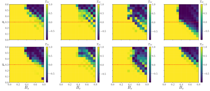
(a)

Figure S5: Representative samples of the topological invariant ($T_{IV}$) for 10 disorder potential components neural network test input and predictions. The first row is $T_{IV}$ resulting from a input disorder potential, and the second row is from the corresponding predicted disorder potential. Each column are the different disorder potential realizations, shown in Fig.5a. The dotted red line corresponds to the conductance profiles in Fig. 5b-e. The topological invariant is plotted for different values of $\mu$ (in meV) and $B_{x}$ (in T).

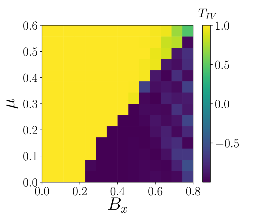
(a)

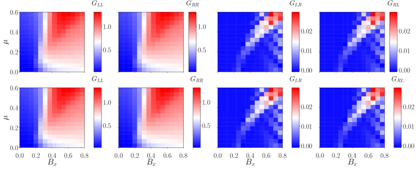
(b)

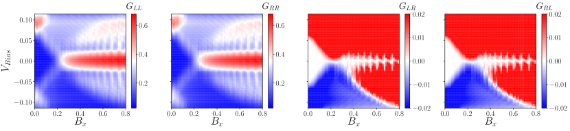
(c)

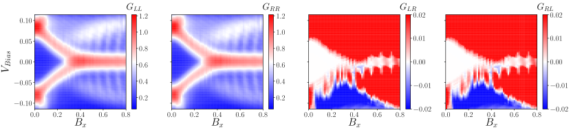
(d)

Figure S6: Pristine sample ($V_{\text{dis}}(x)=0$) topological invariant ($T_{IV}$) and conductance measurements. (a) The topological invariant and (b) Conductance measurements are plotted for different values of $\mu$ (in meV) and $B_{x}$ (in T) at $V_{Bias}=0$. Conductance measurements at (c) $\mu=0$ and (d) $\mu=0.3$ meV are plotted for different values of $V_{\text{Bias}}$ (in meV) and $B_{x}$ (in T). The plots held fixed $\alpha=8\text{meV/nm}$.

References

- [1] (2015) TensorFlow: large-scale machine learning on heterogeneous systems. Note: Software available from tensorflow.org External Links: Link Cited by: §S-II.2.
- [2] (2023) InAs-al hybrid devices passing the topological gap protocol. Physical Review B 107 (24), pp. 245423. Cited by: §S-I.
- [3] (2011) Quantized conductance at the majorana phase transition in a disordered superconducting wire. Physical review letters 106 (5), pp. 057001. Cited by: §S-I.
- [4] (2015) Keras. Note: https://keras.io Cited by: §S-II.2.
- [5] (2014) Kwant: a software package for quantum transport. New Journal of Physics 16 (6), pp. 063065. Cited by: §S-I, §S-I.
- [6] (2010) Majorana fermions and a topological phase transition in semiconductor-superconductor heterostructures. Physical review letters 105 (7), pp. 077001. Cited by: §S-I.
- [7] (2020) Physical mechanisms for zero-bias conductance peaks in majorana nanowires. Physical Review Research 2 (1), pp. 013377. Cited by: Figure S1, Figure S1.
- [8] (2021) Three-terminal nonlocal conductance in majorana nanowires: distinguishing topological and trivial in realistic systems with disorder and inhomogeneous potential. Physical Review B 103 (1), pp. 014513. Cited by: §S-I, §S-I.
- [9] (2011) Scikit-learn: machine learning in python. Vol. 12, JMLR. org. Note: Software available from scikit-learn.org Cited by: §S-II.2.
- [10] (2023) Spectral properties, topological patches, and effective phase diagrams of finite disordered majorana nanowires. arXiv preprint arXiv:2305.07007. Cited by: §S-I.
- [11] (2010) Robustness of majorana fermions in proximity-induced superconductors. Physical Review B 82 (9), pp. 094522. Cited by: §S-I.
- [12] (2021) Charge-impurity effects in hybrid majorana nanowires. Physical Review Applied 16 (5), pp. 054053. Cited by: §S-I.