Soft trade-offs and the stochastic emergence of diversification in E. coli evolution experiments

Abstract

Laboratory experiments of bacterial colonies (e.g., Escherichia coli) under well-controlled conditions often lead to evolutionary diversification in which (at least) two ecotypes, each one specialized in the consumption of a different set of metabolic resources, branch out from an initially monomorphic population. Empirical evidences suggest that, even under fixed and stable conditions, such an “evolutionary branching” occurs in a stochastic way, meaning that: (i) it is observed in a significant fraction, but not all, of the experimental repetitions, (ii) it may emerge at broadly diverse times, and (iii) the relative abundances of the resulting subpopulations are variable across experiments. Theoretical approaches shedding light on the possible emergence of evolutionary branching in this type of conditions have been previously developed within the theory of “adaptive dynamics”. Such approaches are typically deterministic —or incorporate at most demographic or finite-size fluctuations which become negligible for the extremely large populations of these experiments— and, thus, do not permit to reproduce the empirically observed large degree of variability. Here, we make further progress and shed new light on the stochastic nature of evolutionary outcomes by introducing the idea of “soft” trade-offs (as opposed to“hard” ones). This introduces a natural new source of stochasticity which allows one to account for the empirically observed variability as well as to make predictions for the likelihood of evolutionary branching to be observed, thus helping to bridge the gap between theory and experiments.

I Introduction

Understanding the origin and evolution of biological diversity is one of the central issues in evolutionary biology [1, 2, 3]. Historically, diversification was understood almost solely in allopatry, that is, as a consequence of geographical isolation between subpopulations of a common ancestral species [4, 5, 6, 7, 8]. However, the study of sympatric diversification —which does not require spatial segregation— has gained of momentum in recent years. This is due, first, to the mounting empirical evidence both in field and in lab experiments [9, 10, 11, 12, 13, 14, 15, 16, 17, 18, 19, 20, 21, 22] and, second, to the consolidation of the theory of adaptive dynamics as a theoretical framework to tackle this type of evolutionary or eco-evolutionary problems [23, 24, 25, 26, 27, 28, 29, 30, 31].

In the theory of adaptive dynamics, diversification is understood as the consequence of “evolutionary branching” in which two phenotypically-different populations emerge from an ancestral monomorphic one (see [23, 24, 25, 26, 27] and below). Adaptive dynamics assumes that there is a “resident population”, usually considered to be monomorphic, that “mutants” of the dominant phenotype emerge at a small rate —so that ecological and evolutionary processes occur at separate timescales— and the population dynamics depends on the distribution of existing phenotypes. The previous concepts are captured mathematically in the notion of “invasion fitness”, which describes the dependence of the mutant’s growth rate on the resident population. In particular, its sign determines whether the mutant will go extinct or, instead, proliferate, invading the resident population and eventually becoming fixated. Thus, adaptive dynamics can be seen as the gradual phenotypic change of a whole population, that evolves uphill in the fitness landscape. Importantly, due to the frequency-dependent nature of the invasion fitness, the fitness landscape is a dynamical entity, that is, it changes as the population moves in phenotypic space. Typically this evolutionary process ends up finding a (local) maximum of the fitness landscape, at which the population stabilizes. However, sometimes, it may result in the counterintuitive phenomenon of “evolutionary branching” that occurs when the endpoint of the gradient-ascending dynamics —that modifies contemporarily the fitness lanscape itself— is a fitness minimum, rather than a maximum. At this type of “singular point”, the population can only increase its overall fitness by splitting in two sub-populations, where each of them can separately climb one of the sides of the fitness landscape, resulting in a diversification into two different lineages [23, 24, 27, 32, 33].

Adaptive diversification has been empirically observed in a myriad of experiments. For example, isogenic and well-mixed populations of E. coli have been repeatedly observed to evolve into (at least) two coexisting ecotypes with different carbohydrate metabolisms both in chemostat [14, 15, 16] and in serial-dilution (batch) type of experiments [17, 10, 34, 35, 11, 36, 37]. In a chemostat, where the bacterial population is fed solely with glucose in a continuous fashion, one of the emerging subpopulations specializes in consuming glucose, while the second is a scavenger that specializes in the consumption of acetate, a by-product of glucose metabolism. On the other hand, in serial dilution experiments, where both glucose and acetate are added in a cycle of serial dilutions, the difference between the two emerging phenotypes is in the time lag required to switch to acetate consumption when glucose becomes depleted. Two illustrative examples of this are: (i) the work by Treves et al. [16] where the authors report that $6$ out of $12$ independent replicate evolutionary experiments in a chemostat ended up in a stable polymorphism (for up to $1750$ generations); and (ii) the one by Friesen et al. [10] where $5$ out of $12$ independent replicate serial-dilution experiments showed a clear dimorphism after $1000$ generations.

Let us emphasize that, in spite of the stochasticity inherent to mutations, evolutionary branching turns out to be quite reproducible as a substantial proportion of the trials end up in a stable dimorphism [14, 16, 10, 13, 35]. Nevertheless, significant trial-to-trial variability is also observed; in particular: (i) diversification is reported in a large fraction, but not all, of the experiments, (ii) it happens at broadly diverse times, and (iii) the population fraction of the two emerging ecotypes is variable across experiments [16].

Previous theoretical analyses of this problem within the framework of adaptive dynamics have already shown that stylized eco-evolutionary models are able to undergo evolutionary branching under the discussed circumstances [31, 10]. However, these approaches are deterministic in nature and, therefore, predict the occurrence of evolutionary branching in all the realizations or in none of them, depending on some modeling assumptions and/or parameter values. In particular, in order to reproduce branching, previous works assumed, ad hoc, a specific mathematical function to describe a “trade-off function” between the different aspects to be optimized, while other choices did not lead to branching [31, 10].

Trade-offs, sometimes summarized as “you can’t be good at everything” are ubiquitous in ecological and evolutionary modelling (see e.g. [38] and refs. therein). In particular, hard trade-offs, as often imposed in modelling approaches, stem from the idea that evolutionary pressures drive organisms very close to a Pareto front, where improvements in one task come at the price of reducing efficiency in others [38, 39, 40, 41, 42]. In the case under consideration, a specific trade-off curve has been usually assumed between the ability to metabolize the two existing carbon sources (i.e. glucose and acetate). However, the choice of a specific trade-off curve is often the least justified element of mathematical models since —although it is well-founded conceptually [43, 44, 45, 46, 47]— measuring it experimentally is quite a challenging task [48, 49, 50, 51]. Moreover, as extensively discussed in the literature, the assumption of a specific trade-off curve turns out to be critical since it crucially determines whether evolutionary branching occurs or not [24, 52]. An elegant way to circumvent this conceptual difficulty within the framework of adaptive dynamics was proposed by de Mazancourt and Dieckmann [52] who developed a strategy to quantify, for any given eco-evolutionary model, the extent to which the possibility of evolutionary branching is robust as the mathematical shape of the trade-off function is changed (see below).

Our main goal in what follows is to propose a theoretical explanation for the observed variability in the outcomes of well-controlled evolutionary-branching experiments by introducing the idea of a “soft” trade-off —as opposed to the standard “hard” ones— within the framework of adaptive dynamics. By “soft” we mean that the community is not forced to evolve constrained to a precise fixed curve (Pareto front) in phenotypic space, as is the case for hard trade-offs but, rather, it is only constrained to move within a blurrier extended region (see below).

More specifically, in the present work, we introduce an eco-evolutionary model within the framework of adaptive dynamics aimed at describing chemostat experiments although, as we argue, the same ideas could be extended to study serial-dilution experiments. As we shall extensively discuss in what follows, mathematical and computational analyses allow us to show that the model —equipped with a soft trade-off— explains the stochastic emergence of evolutionary branching, in agreement with experimentally observations. Furthermore, it also allows us to make further theoretical predictions for different experimental conditions and allows us to extend the reach of the theory of adaptive dynamics.

The paper is organized as follows: in Section II, the eco-evolutionary model is introduced and the concept of soft trade-offs is defined; in Section III, we present the main results and, finally, in section IV conclusions and future research lines are presented.

II Eco-evolutionary model building

II.1 Ecological dynamics

In order to better understand the outcome of evolution experiments of E. coli on chemostats, we first build a simple though biologically plausible ecological model, following existing modelling approaches [31, 53, 54], capable of describing the bacterial population in quantitative terms and implementing the main relevant features of the experimental systems [14, 15, 16]. In particular it includes the following ingredients and properties:

• An initially isogenic bacterial population, which is maintained in a glucose-limited chemostat [15, 16].

• Due to overflow metabolism (i.e. the phenomenon by which bacteria do fermentation rather than respiration), assimilation of glucose implies excretion of acetate proportionally to the amount of consumed glucose [55, 15].

• The excreted acetate acidifies the medium which leads to an overall slowing down of the total population growth rate [53].

• Even if a strain emerges with the ability to metabolize acetate, owing to the presence of glucose (preferred resource), the consumption of acetate is typically repressed [54].

Considering these ingredients one can write the following set of (deterministic) differential equations for the total number of cells, $N(t)$, and the concentrations of glucose, $G(t)$, and acetate, $A(t)$, respectively, that represent the ecological (not evolutionary) part of the dynamics:

$$\frac{dN}{dt} = \gamma\left(V_{g}\frac{G}{K_{g}+G}+V_{a}\frac{A}{K_{a}+A}\frac{C_{g}}{C_{g}+G}\right)\frac{C_{a}}{C_{a}+A}N-DN$$ (1)

$$\frac{dG}{dt} = DG_{0}-V_{g}\frac{G}{K_{g}+G}N-DG$$ (2)

$$\frac{dA}{dt} = \beta V_{g}\frac{G}{K_{g}+G}N-V_{a}\frac{A}{K_{a}+A}\frac{C_{g}}{C_{g}+G}N-DA.$$ (3)

Observe that all the growth kinetics are described via Monod’s functions [56]. $V_{g,a}$ and $K_{g,a}$ are the maximum growth rate per capita and half-saturation constants on glucose and acetate respectively; $C_{g}$ is the constant controlling the inhibition of acetate consumption due to the repression induced by the presence of glucose; $C_{a}$ is the inhibition of the overall growth rate stemming from the acetate-induced acidification of the medium; $\beta$ determines the fraction of consumed glucose that is excreted in the form of acetate; $\gamma$ is the conversion constant for how much of the consumed resources become biomass; $D$ is the dilution rate of the chemostat; and $G_{0}$ is the glucose concentration in the environment that supplies the chemostat. In what follows, the corresponding numerical values of all these parameters are taken from experimental measurements [14, 15, 16] and are specified in Table 1.

II.2 Evolutionary dynamics

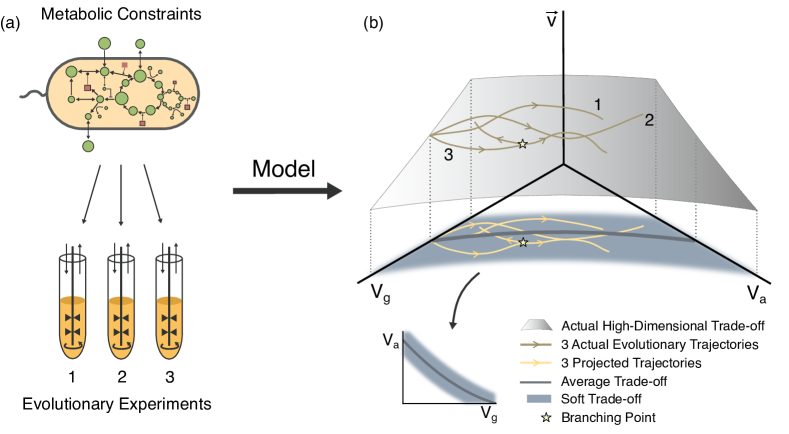
Figure 1: Schematic representation of the concept of soft trade-off. a) Metabolic constraints of bacteria influence the outcome of evolutionary experiments. b) These constraints can be represented by a (topologically complex) manifold (gray shadowed surface), in the multidimensional space formed by all the relevant variables for evolution, which in our case are $V_{g}$, $V_{a}$ and the rest, $\vec{v}$. Starting from the same point, the different evolutionary trajectories corresponding to different realizations of the experiments can move freely in the high-dimensional constraint manifold (golden curves), possibly giving raise to diversification events (yellow star). Thus, the trajectories in the ($V_{g},V_{a}$) plane (yellow lines) are restricted to a certain zone (blue area), but can be different from each other. We model this constraint region, that is, the soft trade-off in the lower-dimensional manifold, by adding a temporarily-correlated noise on top of a certain fixed curve that stands as the average of possible trajectories (inset plot).

In order to determine the full eco-evolutionary model, we still need to formulate its evolutionary dynamics. For this, one must first specify which of the ecological parameters (e.g. constants in Eqs.1-3) are susceptible to be considered as evolving and which ones are kept fixed through the evolutionary process. According to the experimental works [14, 15, 16], it is clear that both of the abilities to feed on glucose and on acetate, respectively, evolve during the course of the experiments. Thus, $V_{a,g}$, $K_{a,g}$ and $C_{g}$ are all susceptible to be chosen as evolving parameters. To keep the model as simple as possible, we choose $V_{g}$ and $V_{a}$, i.e. the maximum growth rate in glucose and acetate respectively and represented generically as $\textbf{V}=(V_{g},V_{a})$, to be the evolutionary parameters: both of them are allowed to vary across generations, so that they determine the metabolic strategy of each strain.

To implement evolution within the framework of adaptive dynamics, one assumes that after having reached the steady state of the ecological dynamics (i.e. a steady state of Eqs.1-3 with $\textbf{V}=(V_{g},V_{a})$), a “mutation”, characterized by a single mutant with a slightly different phenotype $\textbf{V}^{\prime}=(V^{\prime}_{g},V^{\prime}_{a})\neq(V_{g},V_{a})$ is generated. Its invasion fitness, i.e. its per-capita growth rate within the established resident population can be written (from Eq.1) as:

$$f(\textbf{V'},\textbf{V})=\gamma\left(V^{\prime}_{g}\frac{G^{*}}{K_{g}+G^{*}}+V^{\prime}_{a}\frac{A^{*}}{K_{a}+A^{*}}\frac{C_{g}}{C_{g}+G^{*}}\right)\frac{C_{a}}{C_{a}+A^{*}}-D$$ (4)

where $G^{*}$ and $A^{*}$ are the stationary values of the glucose and acetate concentrations, respectively, and depend on the values of both $V_{g}$ and $V_{a}$ of the resident population. Using the formalism of adaptive dynamics, in the (deterministic) limit of small mutations, the evolution in phenotypic space is determined by the canonical equation, describing how the population climbs up the fitness landscape [26, 27, 30]:

$$\frac{d\textbf{V}}{dt}=M\nabla_{\textbf{V'}}f(\textbf{V'},\textbf{V})\Bigr{|}_{\textbf{V'}=\textbf{V}}$$ (5)

where $\nabla_{\textbf{V'}}=[\frac{\partial}{\partial{V_{1}^{\prime}}},\frac{\partial}{\partial{V_{2}^{\prime}}}]$ is the fitness gradient and $\mu$ is the mutation rate, which in the most general case might depend on V and $N$ and in the simplest case adopted here is just a constant.

At this point, one customarily introduces a specific trade-off in the form of a function $V_{a}=h(V_{g})$ which reflects the biological fact that improvement in one “strategy” comes at the price of a loss of efficiency in the other, so that both metabolic strategies cannot be changed in an independent way [38]. This implies that the canonical equation (Eq.(5)) needs to be modified by an additional term to account for such a hard constraint as specified in Methods Sec.VI.1 Eq.(6). By analyzing the fixed points of such an equation, and the properties (first and second derivatives) of such a modified fitness gradient at the fixed points, one could determine whether the course of evolution leads to an evolutionarily stable population, or to the emergence of evolutionary branching. This is typically difficult to accomplish analytically and one usually relies on the analysis of pairwise invasibility plots (see [24, 57] for further information).

However, here we will follow a slightly different (more computational) approach. As stated in the introduction we are interested in explaining properties of the evolutionary experiments such as the time at which a diversification (branching) event occurs and the fraction of the two emerging ecotypes at a certain time. Therefore we need to build an algorithm capable of reproducing actual stochastic evolutionary trajectories, constrained by the fact that their behavior on average is that described by the canonical equation Eq.(6). Such an algorithm, adapted from [58] is fully detailed in Methods Sec.VI.3; in a nutshell, it implies: (i) extending the ecological equations to account for different subpopulations and not just one; (ii) introducing a new equation for a mutant population with a slightly different phenotype from one of the resident subpopulations that is selected with probability proportional to its growth rate at each evolutionary step.

Let us remark that, ideally, one would like to have an individual-based model where each of the individuals could have its own associated phenotype. However, the size of the population, $\sim 10^{13}$, precludes any hope of such a detailed description with the present computational power. Instead, the previously proposed algorithm is an effective “mesoscopic” description, as it does not deal with individuals directly but with “groups” of them (subpopulations) that share the same phenotype; in particular, it allows to describe non-monomorphic populations, i.e. populations distributed in phenotypic space. This type of mesoscopic model, has already been shown to be able to exhibit evolutionary branching when combined with a hard tradeoff (see [31] and the Results section, below).

II.3 Soft trade-offs

As discussed in the introduction and explicitly shown in the Results section, the previously-described eco-evolutionary mesoscopic model coupled with a hard trade-off is deterministic, that is, it either shows branching for every model realization or it does not for any, depending on the specific shape of the considered trade-off curve. Therefore, it is unable to explain the observed variability in the experiments, that is: (i) the fact that diversification is observed in a large fraction, but not all, of the experiments, (ii) it may occur at broadly diverse times, and (iii) the population fraction of the two emerging ecotypes at a certain time is widely variable across experiments.

Let us remark that stochastic effects in the context of adaptive dynamics have already been considered in the literature. Wakano and Iwasa [59] (and more recently some of us [60]) have shown that finite-size effects may prevent the population from undergoing evolutionary branching, even though it is theoretically predicted to emerge at a deterministic level. Similarly, in their seminal paper, Dieckman and Law [26] considered demographic stochasticity in terms of a probability for mutants to become extinct when they first appear. However, both effects become negligible when $\mu N\gg 1$, with $\mu$ being the mutation rate and $N$ the total population, which in our case is a reasonable assumption due to the large population sizes $N\sim 10^{13}$.

Thus, in order to explain the experimental variability, we need to introduce stochasticity in an alternative way. For this, we propose the concept of a soft trade-off in which the population, instead of being forced to live confined within a fixed trade-off curve in phenotypic space, is able to wander stochastically in a wider region with fuzzy boundaries. The idea comes from the appreciation that the trade-off, which gives the effective evolutionary trajectory of the population along a curve in the two-dimensional phenotypic space, might not be identical for every single realization of the experiment [46]. One can rationalize this idea as argued in what follows (see also Fig.1).

The underlying metabolic constraints of bacteria are indeed the same for every realization of the evolutionary experiments. However, such constraints involve complex relations between the many variables that are susceptible to evolution. In our case, we explicitly consider the evolution of $V_{g}$, $V_{a}$ but, in principle, there are many other variables, denoted generically as $\vec{v}$, that could be affected by overall (energetic/metabolic/…) constraints. Such complex relations can be modelled mathematically as a multidimensional constraint manifold (i.e. a high-dimensional “Pareto front” as sketched in Fig.1) [40, 61]. Different realizations of the experiments can then give rise to trajectories that starting from the same point in such a manifold move stochastically within it. Thus, as illustrated in Fig.1, the projected evolutionary trajectories in the two-dimensional $(V_{g},V_{a})$-plane are in general not confined to a one-dimensional curve and may be different for every experimental realization. It is thus reasonable to consider the effect of metabolic constraints more as a “soft” constraint rather than as a strict “hard” one when focusing on the lower-dimensional phenotypic space.

More specifically, to describe soft constraints in a mathematical way, we add a stochastic process or “noise” (modelled as an Ornstein-Uhlenbeck process with amplitude $\sigma$ and temporal correlation $\tau$, as explicitly shown in Methods Sec.VI.2) as an orthogonal perturbation to some central trade-off curve. This curve stands as the average of trajectories and can be chosen with large flexibility without affecting the conclusions (see Sec.VI.2). Depending on the amplitude and temporal correlation of the additional noise, trajectories are constrained to wander at tunable distances of the central trade-off curve.

III Results

III.1 Reproducibility and variability of experimental results

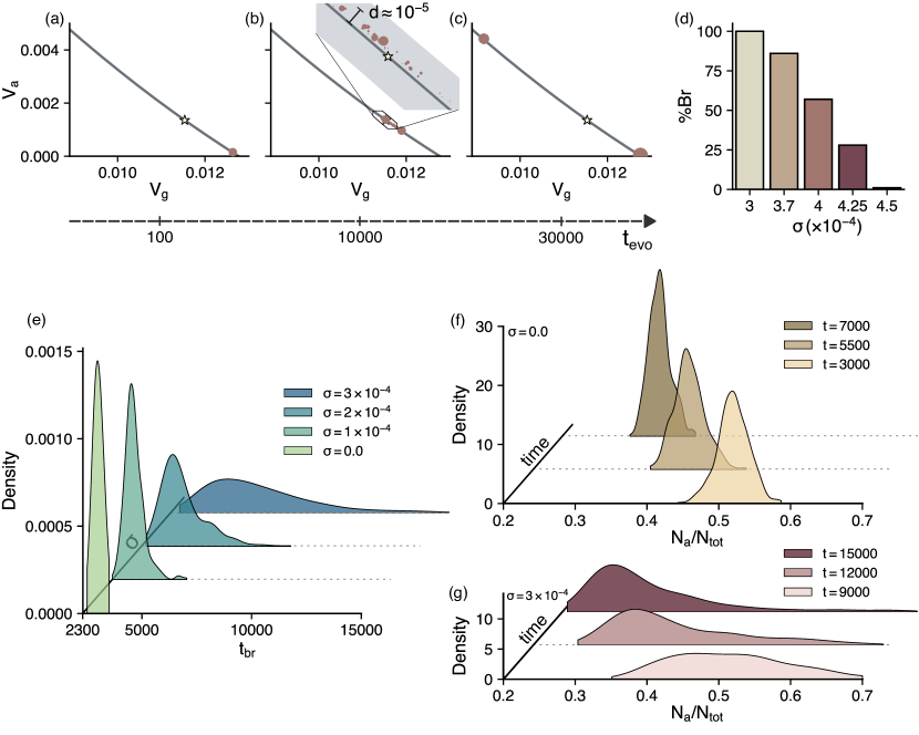
Figure 2: Reproducibility and variability of evolutionary branching in our mesoscopic model with a soft trade-off. a-c) Sub-populations in phenotypic space (represented by a red circle whose radius is proportional to its abundance) for three different times along the evolutionary trajectory, pre-branching (a), during branching (b) and after branching (c), for one specific realization with $\sigma=4\cdot 10^{-4}$. The inset in b) is a zoom in the region close to the branching point (yellow star), where $d\approx 10^{-5}$ is the maximum distance from a subpopulation to the average of the soft trade-off. d) Percentage of realizations (number of them $N_{r}=200$) that undergo evolutionary branching for different amplitudes of the soft trade-off. e-g) Probability density distributions across experiments (number of realizations $N_{r}=500$) of: branching times for different soft trade-off amplitudes (e); and fraction of acetate scavengers at different times for $\sigma=0$ (f) and $\sigma=3\cdot 10^{-4}$ (g) (see Methods Sec. VI.4). System’s parameters for all the plots are: $\beta=0.25$ and those specified in Table 1 where the shown $V_{g/a}$ are rescaled with respect to the table value as $V_{a/g}=\gamma V_{a/g}^{\text{table}}$ with $\gamma=4.5\cdot 10^{10}$. Soft trade-off parameters are: $(a_{tr},b_{tr},c_{tr},\tau)=(83.3,-3.5,0.03,10)$ (see Methods Sec.VI.5 for definitions and further information). Evolutionary simulations are carried out as described in Methods Sec.VI.3.

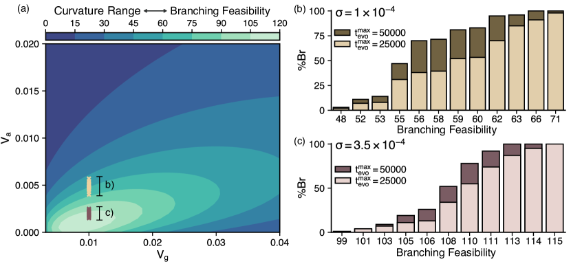
Figure 3: Branching feasibility and the fraction of realizations that undergo branching. a) Branching feasibility plot: contour plot that illustrates in phenotypic space the range of local curvatures of the hard trade-off that allow evolutionary branching. This curvature range can also be interpreted (with the soft trade-off idea) as the likeliness of having evolutionary branching at each point. b-c) Percentage of realizations (total number, $N_{r}=200$) of the eco-evolutionary model with the soft trade-off that undergo evolutionary branching for two different maximum evolutionary times $t_{\text{evo}}^{\text{max}}=2.5\cdot 10^{4}$ and $t_{\text{evo}}^{\text{max}}=5\cdot 10^{4}$ at different points in phenotypic space (that have different curvature range or equivalently different branching feasibility). Points in (b) are those in yellow in panel (a) and $\sigma=10^{-4}$. Points in (c) are those in bourdeaux in panel (a) and $\sigma=3.5\cdot 10^{-4}$. System’s parameters are: $\beta=0.25$ and those specified in Table 1 where the shown $V_{g/a}$ are rescaled with respect to the table value as $V_{a/g}=\gamma V_{a/g}^{\text{table}}$ with $\gamma=4.5\cdot 10^{10}$. Soft trade-off parameters are: $\tau=10$ and the others are obtained for each point shown in panel a) as specified in Methods Sec.VI.5 with $\delta=0.25$. Eco-evolutionary simulations are carried out as described in Methods Sec.VI.3.

As shown in Figure 2, our eco-evolutionary (mesoscopic) model coupled with a soft trade-off is able to account for both the diversification phenomenon as well as the variability evinced in the experiments [16]. Indeed, panels (a-c) show three temporal snapshots of the evolution of the population in phenotypic space for a specific realization of the model with the soft trade-off (as illustrated in the inset of panel b) that ended up diversifying in two highly-specialized sub-populations.

Panel (a) represents the initial phase of the evolutionary picture, in which a glucose-specialist population that produces acetate evolves its ability to assimilate acetate because it is evolutionarily-favoured; panel (b) shows the phase in which the whole population splits in two main ecotypes due to disruptive selection; panel (c) illustrates the last phase in which each of the two ecotypes specializes more and more in metabolizing preferentially one of the two carbon sources, thus giving rise to the two different ecotypes reported in the experiments —the glucose specialist and the acetate scavenger. This evolutionary picture is compatible with the one described in the experiments [15].

Panel (d), in its turn, shows the amount of realizations that, starting from a glucose-specialist population and with the same parameters as in panel (a), ended up undergoing evolutionary branching (at a maximum evolutionary time, arbitrarily fixed to $t_{\text{evo}}^{\text{max}}=3\cdot 10^{4}$) for different amplitudes of the soft trade-off region, which we obtain by varying the noise parameter, $\sigma$, for constant $\tau$. In this way, by tuning the noise amplitude, the model is able to account for the experimental fact that diversification is observed in variable proportion of the experiments. Furthermore, as shown in panels (e-g) the model can also explain the empirically-observed variability in both the branching times and the proportion of acetate scavengers after population splitting. Indeed, panel (e) reveals that branching times —estimated as explained in Methods Sec.VI.4— are variable and their distribution depends on the noise amplitude, $\sigma$. One can observe that, in the case with a ”hard” trade-off (i.e. $\sigma=0$), branching occurs always at the same time (strongly peaked distribution), but the larger the noise $\sigma$ (or equivalently, the amplitude of the trade-off), the wider the distributions of branching times.

On the other hand, Fig.2f shows how the distribution of the fraction of acetate scavengers at different times is quite peaked for the case with the hard trade-off (with a tiny variability that stems from the intrinsic randomness of the mutation procedure, see Methods Sec.VI.3), whereas the case with a non-vanishing amplitude of the trade-off, Fig.2g, shows a much wider distribution. Therefore, assuming the data could be explained with a hard trade-off, one should see practically the same fraction for different realizations if measured at the same times, whilst assuming a soft trade-off, one should observe significant differences even if measured at same times. Although experimental data for branching times and fractions is scarce to allow for a quantitative comparison, our results suggest that the empirical observations are best represented by the noisy case [16].

III.2 Branching feasibility and trade-off (in)dependence

As already discussed in the introduction, the specific evolutionary outcomes of eco-evolutionary models depend crucially on the form of the trade-off [24, 52]. Therefore, in order to generalize the results found in Sec.III.1 without relying on a specific form of the (mean) trade-off curve, one needs a framework that is able to discern whether a given ecological model equipped with a certain set of parameter values, is able to undergo evolutionary branching (or not) independently of the specific form of the trade-off.

To this aim, we make use of the formalism proposed by de Mazancourt and Dieckmann [52]. As originally developed, such a framework allows one to analyse geometrically the possible evolutionary outcomes that can occur in the deterministic setting without imposing a specific mathematical function for the trade-off (for the sake of completeness, an overview of the method is described in Methods Sec.VI.1). In particular, within this formalism one can construct plots such as that of Fig. 3a, providing information on how independent is evolutionary branching on the specific mathematical form of the hard trade-off. More specifically, it gives at each point in phenotypic space, a measure of the range of possible local curvatures of the hard trade-off function that allows the model to undergo evolutionary branching at such a point, thus quantifying the robustness of branching against changes in the trade-off function. Then, for example, in regions where the range of possible local curvatures is small (deep blue in Fig. 3a), the model undergoes evolutionary branching deterministically in that region only for very specific (fine-tuned) trade-off curves, whereas in regions where such curvature range is high (light green in Fig. 3a), evolutionary branching occurs deterministically for a larger family of possible trade-off functions (see Section VI.1 for further details).

Nevertheless, let us recall again that depending on the specific form of the trade-off, branching happens or does not happen in a deterministic way. Therefore, we would like to see how this formalism could be reinterpreted when we include the idea of soft trade-offs. It turns out that using soft trade-off, the previous plots (e.g. Fig.3a) can be interpreted as “evolutionary-branching feasibility plots”, i.e.graphs showing the regions in phenotypic space where it is more likely to see an evolutionary branching event. In other words, regions in phenotypic space where branching is more robust against changes in the specific form of the hard trade-off correspond to regions in phenotypic space where branching is more likely to happen with the soft (stochastic) trade-off and vice-versa.

To justify this claim, we employ without loss of generality our eco-evolutionary model with a certain soft trade-off, whose average curve (i.e. in the $\sigma=0$ limit) produces branching deterministically at a selected point in phenotypic space (see Methods Sec.VI.2 for further details on how the soft trade-off is built). Then, as illustrated in Fig.3b-c, points where deterministic branching is more independent on the specific form of the hard trade-off —i.e. points where the range of local curvatures of the hard trade-off that allow branching is larger— correspond in the soft trade-off case to more realizations that end up experiencing diversification at that point and vice-versa.

Let us however remark, that this mapping between curvatures range and feasibility of branching is quantitatively conditioned by the maximum evolutionary time of the realizations, $t_{\text{evo}}^{\text{max}}$. As both panels (b) and (c) show, the higher $t_{\text{evo}}^{\text{max}}$, the larger is the possibility to observe evolutionary branching. This fact —i.e. the increase in the number of experiments that show diversification with the duration of such experiments— is indeed observed also experimentally [16]. Furthermore, Fig.3b-c illustrates that the mapping is also quantitatively affected by the amplitude of the soft trade-off (controlled by $\sigma$). In agreement with Fig.2d, the smaller the $\sigma$, the higher the possibility of having evolutionary branching. In fact, in the hard trade-off limit where $\sigma=0$ and the trade-off reduces to its average curve (which is chosen such that it undergoes branching), evolutionary branching occurs deterministically at almost the same times and for low evolutionary times, $t_{\text{evo}}<2000$, independently of the point in phenotypic space (data not shown).

Therefore, interpreting Fig.3a as a branching-feasibility plot, we observe that branching is more likely for low values of $V_{a}$, which agrees with the reported picture of the evolution experiments given in [15]. As shown in Sec.III.3, the specific contour pattern depends highly on the conditions of the experiment, that is, the concentration of glucose in the environment supplying the chemostat, $G_{0}$, the dilution rate, $d$, and the proportion of the consumed glucose that gets excreted as acetate, $\beta$. Thus, Fig.3a reveals essentially that the system, under these specific environmental conditions, is rather likely to undergo evolutionary branching, which justifies its observed repeatability in actual experiments.

III.3 Theoretical predictions for different experimental values

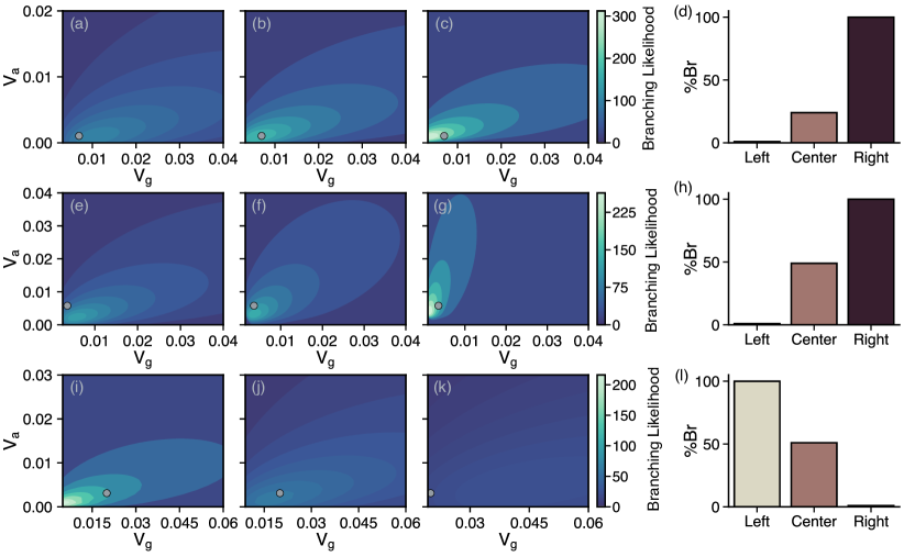
Figure 4: Branching feasibility and the percentage of realizations that undergo branching for different experimental conditions. a-c) Branching-feasibility plots for different values of glucose concentration in the environment supplying the chemostat: $G_{0}=260$ (a), $G_{0}=694$ (b) and $G_{0}=3469$ (c), all of them in $\mu$mol/L. d) Number of realizations that undergo branching at the point depicted in a-c) for the same soft trade-off with $(a_{tr},b_{tr},c_{tr},\tau,\sigma)=(88.2,-2.5,0.014,10,6\cdot 10^{-4})$ (see ’Soft trade-offs’ in Materials and Methods for definitions and further information). e-g) Branching-feasibility plots for different values of acetate concentration in the environment supplying the chemostat: $A_{0}=100$ (e), $A_{0}=260$ (f) and $A_{0}=1000$ (g), all of them in $\mu$mol/L. h) Number of realizations that undergo branching at the point depicted in e-g) for the same soft trade-off with $(a_{tr},b_{tr},c_{tr},\tau,\sigma)=(164.3,-3.6,0.011,10,5\cdot 10^{-4})$. i-k) Branching-feasibility plots for different values of the dilution rate: $D=0.0015$ (i), $D=0.006$ (j) and $D=0.015$ (k), all of them in 1/min. l) Number of realizations that undergo branching at the point depicted in i-k) for the same soft trade-off with $(a_{tr},b_{tr},c_{tr},\tau,\sigma)=(65.5,-5.6,0.088,10,1.2\cdot 10^{-4})$. Total number of realizations for the histograms is $N_{r}=200$. The remaining parameters specified in Table S1 in the supplementary material where the shown $V_{g/a}$ are rescaled with respect to the table value as $V_{a/g}=\gamma V_{a/g}^{\text{table}}$ with $\gamma=4.5\cdot 10^{10}$.

As shown, our mesoscopic model equipped with soft trade-offs is able to explain both the repeatability and variability observed in the experiments. Can it also be employed to make theoretical predictions? To do so, we computed the branching-feasibility plots for experimental conditions that are different from those reported in the available experiments (see Fig.4).

First of all, Fig.4a-c shows clearly how higher concentrations of glucose in the environment supplying the chemostat, $G_{0}$, imply in general a larger likeliness for branching to occur. Indeed, we verify this in Fig.4d. As in Fig.3b-c, we use for the three different environments a certain soft trade-off whose average curve produces deterministic branching at a selected point. As one can clearly see in the histogram, the higher is the supply of glucose, the larger the amount of realizations that undergo evolutionary branching. Moreover, the similarity in the shape of the contour pattern with the one in Fig.3a is related to the fact that the proportion of available acetate (i.e. $\beta$ in this case) is the same as in that case.

On the other hand, if an acetate concentration, $A_{0}$, is added to the media supplying the chemostat (Fig.4e-g), the pattern in the contour plot shifts, and the likeliness of having branching increases to some degree but in different areas. The shifting takes place because the added concentration of acetate increases the proportion of available acetate (i.e. $\beta+A_{0}/G_{0}$). Again, we compare the amount of realizations that undergo branching for the same soft trade-off in the three different environments in Fig.4h, showing that the case with higher supply of acetate is more likely to undergo branching.

Finally, one can appreciate that the dilution rate $D$ is also a relevant parameter for the emergence of branching (Fig.4i-k). In particular, higher values of $D$ dramatically reduce the possibilities of having branching as illustrated in Fig. 4l.

Summing up, our reinterpretation of the formalism developed by de Mazancourt and Dieckmann [52] with the soft trade-off, not only generalizes our results for a more general set of trade-offs but also allows us to compare the possibility of observing branching for different experimental conditions, which gives a deeper understanding of the theoretical reasons for branching and it may help to make closer contact and predictions for future experiments.

IV Discussion

Understanding the mechanisms that generate, promote and stabilize biological diversity stands as a challenging task. Microbiology experiments are particularly suited for this since the rapid adaptation/evolution of microorganisms allows one to empirically study evolution over relatively short time periods [62]. Here, we focused on a particular type of experimental setup in which a well-mixed isogenic population of E. coli is maintained on a glucose-limited chemostat over thousands of generations [14, 15, 16]. After a sufficient number of generations, a number of different experimental works report a splitting of the ancestor lineage into two different ecotypes (or strains) distinguished by their carbohydrate metabolism: the first one specialises in the consumption of glucose while the second consumes preferentially a byproduct of glucose metabolism, i.e. acetate. This constitutes an illustrative example of the emergence of cross-feeding and the generation of complex communities/ecosystems even in the presence of few resources [54, 63].

Previous work [31] showed, in the context of adaptive dynamics, that a simple eco-evolutionary model can explain in a parsimonious way such a diversification event as evolutionary branching, by assuming a specific (hard) trade-off function between the evolving phenotypes (i.e. glucose and acetate). Nevertheless, such an approach is deterministic in nature, i.e. either predicts that branching should be observed always or never depending on the specific trade-off form chosen. Therefore it is unsuited to explain the empirically observed stochasticity in the experiments, that is, the common (not deterministic) emergence of diversification and the variability both in branching times and in the relative weights of the emerging populations.

Alternatively, in this work, we propose the idea of a soft trade-off that stands as an effective representation of the underlying metabolic relations that constrain the evolution of bacteria in a high-dimensional phenotypic space. Instead of forcing the evolutionary trajectories in a lower-dimensional phenotypic space to a certain fixed curve, it allows the populations to move in a wider region in such a space, introducing a new source of stochasticity along such a space. Mathematically, the soft trade-off is characterized by a central curve that stands as the average of the different trajectories, the correlation time, $\tau$, that defines how fast the trajectories go back to this average curve and its amplitude, which for fixed $\tau$ is determined by $\sigma$ and defines the width of the (fuzzy) region where populations can evolve.

Thus, we have built a biologically plausible mesoscopic eco-evolutionary model (see Eqs.1-3), fed with experimentally measured parameters (see Table 1 in Materials and Methods) and equipped with the mentioned soft trade-off. We have shown that such a model is indeed able to account for the variability reported in the experiments (Fig.2). In particular, contrary to existing models it does reproduce: (i) the fact that branching occurs in a large proportion, but not all, of the realizations (Fig.2a-d) (ii) it may happen at considerably different times (Fig.2f) and (iii) the fraction of acetate scavengers at a certain time are variable across experiments (Fig.2g-h).

Moreover, reinterpreting the formalism of de Mazancourt and Dieckmann [52] with the idea of the soft trade-off, we have also generalized our results for a larger family of trade-offs. More specifically, we have been able to build what we termed the “branching-feasibility plot” for our model (Fig.3a), which quantifies, for the different points in phenotypic space, the possibility of branching for a fairly general set of possible soft trade-offs. Indeed, we have verified this by plotting, for different points in phenotypic space, the number of realizations that undergo evolutionary branching (Fig.3b-c). Moreover, we have shown that this number of realizations is affected by both the amplitude of the soft trade-off and the maximum evolutionary time of the specific realization. More specifically, the smaller the amplitude and the higher the maximum evolutionary time, the higher the number of realizations that undergo branching. In conclusion, the branching-feasibility plot reveals that for a large set of soft trade-offs, this type of chemostat system is fairly likely to undergo a diversification event, all the most for low values of $V_{a}$, justifying its repeated, although variable, emergence in actual experiments.

It is also noteworthy, that the framework we have devised here allows to make theoretical predictions for the possibility to observe branching for different experimental conditions. Indeed, in Fig.4, we show how for different experimental parameters, branching can be made more (or less) likely and that the region in phenotypic space where it is most likely can vary. In particular, we have shown that by increasing the amount of glucose and/or acetate supplied to the system, evolutionary branching is more likely to be observed whereas augmenting the dilution rate can make branching almost impossible. In this way, our framework provides a deeper theoretical understanding of the underlying reasons controlling diversification in real experiments. Furthermore, these predictions, can easily be tested experimentally by repeating the evolutionary experiments under different conditions and compare the percentage of realizations that end up diversifying.

Let us remark that the theoretical analyses made in this work assume, as customarily in adaptive dynamics, that evolutionary changes are perturbative in phenotypic space, i.e. phenotypes change gradually. However, this might not be the case for actual evolutionary experiments with bacteria. For example, one can imagine that mutations in certain genes could confer an initially glucose-limited bacteria population the ability to metabolize finite amounts of acetate without having to wait for many generations. Future work will therefore be devoted to implementing this possibility in the models and exploring how it can possibly change the overall picture. Note in particular that extensions of adaptive dynamics accounting for non-perturbative mutations are presently under development [60]. Finally, as mentioned in the introduction, the repeated branching of an ancestor E. coli lineage into two distinct ecotypes characterized by their carbohydrate metabolism is also observed in serial dilution experiments in which bacteria evolve in a batch of glucose-acetate [17, 10, 34, 35, 11, 36, 37]. The framework introduced here can be easily adapted to such a scenario and further work will be devoted to it. We believe that the ideas introduced here —in particular the idea of soft trade-offs— will motivate further research into understanding the underlying principles of evolution under controlled conditions.

V Acknowledgements

This work has been supported by (i) grant PID2020-113681GB-I00 of the Spanish Ministry and Agencia Estatal de Investigación (MCIN/AEI/10.13039/501100011033) with European Regional Development funds (ERDF) ”A way of making Europe”, and Consejería de Conocimiento, Investigación Universidad, Junta de Andalucía and Universidad de Granada under project B-FQM-366-UGR20 (ERDF). R.C.L. acknowledges funding from the Spanish Ministry and AEI, under Grant No. FPU19/03887 and from the Arqus alliance of european universities program 6.5. SS and SA acknowledge the support of the NBFC to the University of Padova, funded by the Italian Ministry of University and Research, PNRR, Missione 4 Componente 2, “Dalla ricerca all’impresa”, Investimento 1.4, Project CN00000033. The authors warmly thank Amos Maritan for insightful discussions and for contributions to the early stages of this research.

VI Methods

VI.1 Evolution of a monomorphic population subject to a trade-off

We briefly review here the geometrical method developed in [52, 64, 65] where the evolutionary outcomes of the evolution of a monomorphic population in a 2-D phenotypic space can be characterized without specifying a particular trade-off beforehand. This method has also been extended partially to dimorphic populations by [66] and to multidimensional phenotypic spaces by [30]. In the following we work with a monomorphic population with two evolving phenotypes and assume the reader is familiar with the framework of adaptive dynamics which can be found in e.g. [27].

Under frequency-dependent selection, two independent properties have to be considered: (i) evolutionary stability, i.e. strategies that cannot be invaded once established and (ii) convergence stability, i.e. strategies toward which directional evolution will converge through small evolutionary steps. Thus, four possible evolutionary outcomes exist depending on whether convergence or evolutionary stabilities are achieved or not, but we are mostly interested in two: continuously stable strategies that share both convergence and evolutionary stability and evolutionary branching points that have convergence but not evolutionary stability (Fig.5b). Conventional analyses of evolutionary models require ad hoc assumptions about the shape of the trade-off curves. This method, however, offers a geometric representation of evolutionary and convergence stabilities, thus enabling the visualization of how evolutionary outcomes depend on arbitrary trade-offs in an simple way. Therefore, with this method one can easily identify the possible evolutionary outcomes that general trade-offs can induce and determine the effect on them of ecological parameters independently of the specific trade-off curve.

Populations are represented in phenotypic space as points whose location correspond to the resident phenotype. Evolution and selection change the population’s phenotype over time making the point to describe a trajectory in phenotypic space (evolutionary trajectory). In the absence of frequency-dependent selection, a single fitness value can be assigned to each phenotype, resulting in a fixed fitness landscape [67]; a population then just climbs up its fitness landscape until it reaches a maximum. By contrast, under frequency-dependence, where a fixed fitness landscape is absent, one relies instead on the notion of invasion fitness $f(\textbf{x}^{\prime},\textbf{x})$, which is simply the per capita growth rate of the mutant’s phenotype, $\textbf{x}^{\prime}$ in the environment determined by the resident phenotype x. If $f(\textbf{x}^{\prime},\textbf{x})$ is positive $\textbf{x}^{\prime}$ can initially invade into a population dominated by x; otherwise, it cannot. Directional evolution is thus inferred from local selection gradients, $\textbf{g}(\textbf{x})=(g_{1}(\textbf{x}),g_{2}(\textbf{x}))=\nabla_{\textbf{x}^{\prime}}f(\textbf{x}^{\prime},\textbf{x})|_{\textbf{x}^{\prime}=\textbf{x}}$, which describe the most-favoured direction by selection around a population’s resident phenotype.

Indeed, the phenotype x evolves according to the canonical equation (Eq.(5)), i.e. it attempts to climb the local selection gradient $d\textbf{x}/dt\propto\textbf{g}(\textbf{x})$ [26]. Nevertheless, the presence of a trade-off between the evolving phenotypes, that can be written in general as $H(\textbf{V})=0$, constrains the evolution to the projection of the gradient onto the trade-off curve [30]:

$$\frac{d\textbf{V}}{dt}=\mu\left(\nabla_{\textbf{V'}}f(\textbf{V'},\textbf{V})\Bigr{|}_{\textbf{V'}=\textbf{V}}-\frac{\nabla H(\textbf{V})\cdot\nabla_{\textbf{V}^{\prime}}f(\textbf{V'},\textbf{V})\Bigr{|}_{\textbf{V'}=\textbf{V}}}{|\nabla H(\textbf{V})|^{2}}\nabla H(\textbf{V})\right)$$ (6)

where $\mu$ is the evolutionary rate coefficient, that in the most general case might depend on V and $N$, and $\nabla_{\textbf{V'}}=[\frac{\partial}{\partial_{V_{1}^{\prime}}},\ldots,\frac{\partial}{\partial_{V_{P}^{\prime}}}]$, where $P$ is the dimension of the phenotype space.

In the two-dimensional case under consideration, one has that $\textbf{x}=(x_{1},x_{2})$ and $x_{2}=h(x_{1})$ where $h$ is an arbitrary trade-off function. If evolution is constrained to follow a hard trade-off curve, it reaches an endpoint (singular point) if at some point the selection gradient is perpendicular to the tangent vector of the trade-off function, h, i.e. $\textbf{g}\cdot\textbf{h}=0$ (see points A and B in 5a). Therefore, one can construct curves that, at any point in phenotypic space, are orthogonal to the local selection gradient and hence to all resultant evolutionary trajectories. These curves (blue lines in 5a), called A-boundaries, are then independent from the trade-off and depend exclusively on the characteristics of the model. Is only when we are to find the specific fixed point(s) of the evolutionary dynamics that we have to specify the trade-off function. Singular points can then be seen as those in which the slopes of the A boundary, $S_{A}$, and the trade-off function, $S_{T}$, are equal or equivalently when both curves are tangent to each other. Besides, A boundaries help to distinguish in a simple geometrical way whether the fixed point is convergence stable, and as such no neighbouring phenotypes can be reached by directional evolution, (A point in Fig.5a) or unstable, where neighbouring phenotypes can indeed be reached by evolution, (B point in Fig.5a).

To asses evolutionary stability, a second type of curve, the so called local I-boundary (red dashed lines in Fig.5a), is needed. For any point in phenotypic space, x, the local I curve separates regions of mutant phenotypes $\textbf{x}^{\prime}$ that can invade into a population situated at x, $f(\textbf{x}^{\prime},\textbf{x})>0$, from those that cannot, $f(\textbf{x}^{\prime},\textbf{x})<0$. The local I boundary is then defined as all $\textbf{x}^{\prime}$ with $f(\textbf{x}^{\prime},\textbf{x})=0$. Notice that at x both A and I boundaries have the same slope, $S_{A}=S_{I}$. Indeed, at x, the slope of the A boundary, $S_{A}=-g_{1}(\textbf{x})/g_{2}(\textbf{x})$, can be obtained from its tangent vector, $\textbf{t}_{A}(\textbf{x})=\pm(g_{2}(\textbf{x}),-g_{1}(\textbf{x}))$, which is nothing but the perpendicular to the selection gradient, $\textbf{g}(\textbf{x})$. On the other hand, the slope of the local I boundary at $\textbf{x}^{\prime}=\textbf{x}$ can be obtained as the slope of the implicit curve, $f_{\textbf{x}}(\textbf{x}^{\prime})\equiv f(\textbf{x}^{\prime},\textbf{x})=0$, which is nothing but $S_{I}=-\partial_{x_{1}^{\prime}}f(\textbf{x}^{\prime},\textbf{x})/\partial_{x_{2}^{\prime}}f(\textbf{x}^{\prime},\textbf{x})|_{\textbf{x}^{\prime}=\textbf{x}}\equiv-g_{1}(\textbf{x})/g_{2}(\textbf{x})$.

At a singular point a resident population lying on a trade-off curve experiences disruptive selection (evolutionary instability) if its invader set (i.e. $\textbf{x}^{\prime}\mid f(\textbf{x}^{\prime},\textbf{x})>0$) includes the surrounding trade-off curve (B in Fig.5a). By contrast, if the trade-off curve does not fall into the invader set, selection on the singular point is stabilizing (A in Fig.5a).

Thus, the relative local curvatures of A-boundaries, I-boundaries, and trade-off curves at singular points determine the different possible evolutionary outcomes. In order to compare the curvatures, a convention is needed. Since, by definition, the local selection gradient at a singular point is perpendicular to the local I-boundary, A-boundary, and trade-off curve: we define positive curvature when looking along the local selection gradient the curve is convex, otherwise the curvature is negative. Denoting the curvatures of the A, I boundaries and the trade-off by $C_{A}$, $C_{I}$ and $C_{T}$ respectively we can then conclude that a singular phenotype is convergence table (unstable) if $C_{T}<C_{A}$ ($C_{T}>C_{A}$) and locally evolutionary stable (unstable) if $C_{T}<C_{I}$ ($C_{T}>C_{I}$). Thus, the continuously convergence strategy and evolutionary branching points can be easily distinguished (see Fig.5b). Analytical details corresponding to these geometric insights are provided in [52].

To discriminate the conditions for which an initially monomorphic population can become polymorphic. For this the initial point in phenotypic space must converge to an evolutionary branching point which, as we have shown, requires $C_{I}<C_{T}<C_{A}$. One can therefore visualize where in phenotypic space evolutionary branching is more independent from the trade-off by plotting at each point the difference $C_{A}-C_{I}$ (see Fig.3a in the main text).

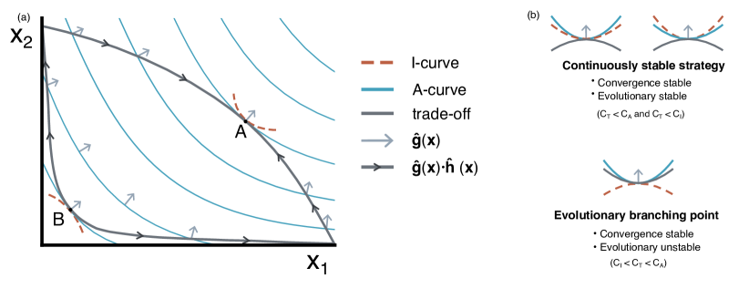
Figure 5: Geometric analysis of the possible evolutionary outcomes. a) An example of A-curves (blue lines), local I-curves (red dashed lines) and possible trade-offs (dark grey lines). The direction of the selection gradient $\textbf{g}(\textbf{x})$ (light grey arrows) and its projection onto the trade-off curves $\hat{\textbf{g}}(\textbf{x})\cdot\hat{\textbf{h}}(\textbf{x})$ (dark grey arrows) are shown to indicate the direction of selection. Singular points where the trade-off is perpendicular to the A-curve are shown in A and B. As can be seen by the direction of the arrows inside the trade-off, the former (A) is convergence stable, whereas the latter (B) is not. Besides, A is evolutionary stable since the I-curve is over the trade-off at that point whilst B is not because the I-curve is under the trade-off. b) Geometric signatures of two possible evolutionary outcomes.

VI.2 Soft trade-offs

To define the soft trade-off we first need to choose its average curve. We want the soft trade-off to give rise to evolutionary branching, therefore we shall select the average curve with the right properties to produce it. For this, we only need to define its curvature and slope at a certain point, which is the evolutionary branching point in the deterministic case (see Sec. VI.1). Therefore, any curve that has a non trivial second order Taylor expansion at that point could be of use. To make it as simple as possible but without loss of generality, we use a second order polynomial:

$$V_{a}^{tr}(V_{g})=a_{tr}V_{g}^{2}+b_{tr}V_{g}+c_{tr}$$ (7)

where the coefficients are defined such that at a certain point the polynomial has a certain curvature and slope. In particular at that point (see Sec. VI.1):

• The curvature $C_{T}$ has to be in the range $(C_{I},C_{A})$ where $C_{I}$ and $C_{A}$ are the curvatures of the I and A-curves (see Sec. VI.1). Due to the specific form of our invasion fitness, in our case $C_{I}=0$ always, so $C_{T}=\delta C_{A}$ where $\delta\in(0,1)$.

• The slope $S_{T}$ must be equal to that of the A-curve $S_{A}$, so $S_{T}=S_{A}$.

• Trivially, the curve must contain the point.

Thus, denoting the selected point as $(V^{s}_{g},V^{s}_{a})$, the coefficients become:

$$a_{tr} = \frac{1}{2}\delta C_{A}(1+S_{A}^{2})^{\frac{3}{2}}$$ (8)

$$b_{tr} = S_{A}-2a_{tr}V^{s}_{g}$$ (9)

$$c_{tr} = V^{s}_{a}-b_{tr}V^{s}_{g}-a_{tr}{V^{s}_{g}}^{2}$$ (10)

Let us remark that these coefficients define not a single valid curve but a family of them since $\delta\in(0,1)$ is not fixed. Furthermore, as already stated before any other more complex curve with a local Taylor expansion similar to Eq.(7) would also be suitable. Thus, our results can be extrapolated for a general set of average trade-off curves. However, let us note that when changing the curve, one must pay attention to avoid a curve with additional singular points (i.e. those at which evolution ends, see Sec. VI.1) that come before in the evolutionary trajectory. These singular points can be detected by plotting the so-called pairwise invasibility plots (further details in [24, 57]).

Finally, to fully determine the soft trade-off, we have to establish how the evolutionary trajectories move in the direction perpendicular to the average trade-off curve. For this, we define the distance to the average trade-off curve at each evolutionary time-step as a temporally correlated function of the distance in the previous time. Essentially, is a time-discrete Orstein-Uhlenbeck process with $\Delta t=1$ and zero average. Thus we have:

$$d_{t+1}=(1-\frac{1}{\tau})d_{t}+\sqrt{\frac{1}{\tau}}\xi$$ (11)

where $\tau$ is the correlation time of the Ornstein-Uhlenbeck process that determine how fast the process return to the average curve (i.e to $d=0$) in the absence of the noise and $\xi$ is a random Gaussian variable of zero average and standard deviation $\sigma$ which, for fixed $\tau$, determines the amplitude (in phenotypic space) of the soft trade-off.

VI.3 Evolutionary algorithm

Here we follow a slightly modified version of the evolutionary algorithm employed in [58]. To simulate the evolution of the whole population, one needs first to extend the system of ecological dynamics Eqs.(1-3) for an arbitrary number M of sub-populations:

$$\frac{dN_{j}}{dt} = \gamma\left(V^{j}_{g}\frac{G}{K_{g}+G}+V^{j}_{a}\frac{A}{K_{a}+A}\frac{C_{g}}{C_{g}+G}\right)\frac{C_{a}}{C_{a}+A}N_{j}-DN_{j}$$ (12)

$$\frac{dG}{dt} = D(G_{0}-G)-\sum_{j}V^{j}_{g}\frac{G}{K_{g}+G}N_{j}$$ (13)

$$\frac{dA}{dt} = \beta\sum_{j}V^{j}_{g}\frac{G}{K_{g}+G}N_{j}-\sum_{j}V^{j}_{a}\frac{A}{K_{a}+A}\frac{C_{g}}{C_{g}+G}N_{j}-DA$$ (14)

where $j=1,\ldots,M$ is the sub-population index. Starting from a single monomorphic population, so that $M=1$, one integrates the previous of equations until a steady state is reached. After that, if any of the existing sub-populations falls below a small extinction threshold density (arbitrarily fixed to $n_{min}=10^{-6}$), it is removed from the system. Then, a new “mutant” subtype is split from one of the resident sub-types, characterized by $(V_{g},V_{a})$ that is randomly chosen with probability proportional to its total growth rate in the steady state.

To obtain the mutant phenotype $(V^{\prime}_{g},V^{\prime}_{a})$ we have to distinguish which kind of trade-off is being used. (i) In the case of the stochastic trade-off, we first determine the distance $d_{old}$ between the point $(V_{g},V_{a})$ and its closest point in the average trade-off curve, $(V^{closest}_{g},V^{closest}_{a})$ (see Fig.6). Then, we add a random mutation, $\xi_{1}$, selected from an uniform distribution in the range $[-m,+m]$ with $m=10^{-4}$, to $(V^{closest}_{g},V^{closest}_{a})$ and obtain the point that is at arc-length distance $\xi_{1}$ in the average curve from it (see Fig.6). Thus, one arrives to a point in the curve that we denote $(V^{\prime closest}_{g},V^{\prime closest}_{a})$. Finally, we obtain the mutant phenotype by using the temporarily-correlated noise (soft trade-off), as the point that is at distance $d_{new}=(1-\frac{1}{\tau})d_{old}+\sqrt{\frac{1}{\tau}}\xi_{2}$ from $(V^{\prime closest}_{g},V^{\prime closest}_{a})$ where $\xi_{2}$ is selected from a zero-averaged Gaussian distribution with standard deviation $\sigma$. (ii) On the other hand, in the case of a hard trade-off we determine the mutant phenotype as $V^{\prime}_{g}=V_{g}+\xi_{1}$ and $V^{\prime}_{a}=h(V^{\prime}_{g})$ with $\xi_{1}$ is defined as above and $h$ being the hard trade-off function.

Once the mutant is obtained, its population is set to be the $10\%$ of the ancestral one, which in turn gets reduced by $10\%$. Moreover, in order to reduce computational complexity, once each $\Delta t_{merge}=100$ we discretize the phenotypic space in squares of width $m$ and merge the subpopulations that fall in the same bin by summing their populations and averaging its $V_{g}$ and $V_{a}$ values.

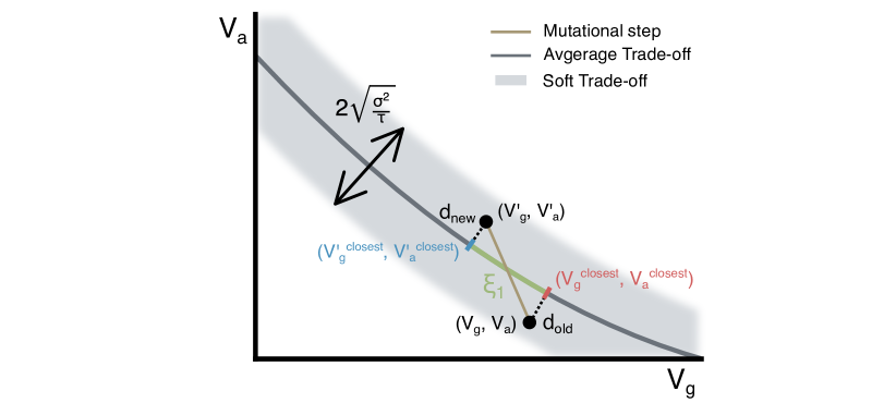
Figure 6: Representation of one mutational step of the evolutionary algorithm. In colours are represented the auxiliary variables needed to get the mutational step from the resident population at $(V_{g},V_{a})$ to the mutant at $(V^{\prime}_{g},V^{\prime}_{a})$. The soft trade-off (grey fuzzy region) and its average (dark grey curve) are also depicted with the magnitude of its amplitude $2\sqrt{\sigma^{2}/\tau}$.

VI.4 Branching time determination

To determine branching times, at each evolutionary time, we pick from the $M$ subpopulations with phenotypes $\{(V^{1}_{g},V^{1}_{a}),(V^{2}_{g},V^{2}_{a}),\ldots,(V^{M}_{g},V^{M}_{a})\}$ the subpopulation with the maximum $V^{\text{max}}_{g}$ and create a set initially containing only such value. Likewise with the minimum $V^{\text{min}}_{g}$. Then, we add to the set of the maximum (minimum) those subpopulations with $V_{g}$ at arc-length distance inside the curve below $d=6\cdot 10^{-4}$ from the maximum (minimum). In this way, we fix a criterion to declare that branching has occurred if the two groups are disjoint and take the evolutionary time when this happens as the branching time. Besides, we denote the group with higher $V_{g}$ as the glucose specialist and the other —that have a lower $V_{g}$ and in turn a higher $V_{a}$— as the acetate scavengers.

VI.5 Evolutionary branching with a soft trade-off

In order to demonstrate that the evolutionary-branching feasibility plot (Fig.3a) does indeed shows where in phenotypic space is more likely to have branching, we showed the percentage of realizations that end up causing branching at the specified points in phenotypic space (Fig.3b). Here we explain how we have obtained Fig.3b: (i) we choose an average curve of the soft trade-off that has the right properties to deterministically (in absence of the soft trade-off amplitude, that is, $\sigma=0$) originate evolutionary branching at a certain point, $\textbf{V}^{s}=(V^{s}_{g},V^{s}_{a})$ (for example the points marked with a cross in Fig.3a). This can be easily done as detailed in Methods Sec. VI.2. (ii) Then, once we have the soft trade-off defined with a certain $\sigma$ and $\alpha$, we initiate the evolutionary algorithm with a monomorphic population whose phenotype, is equal to that of the selected point, $\textbf{V}^{\text{init}}=\textbf{V}^{s}$. We do it in this way to be able to compare the branching times for the different point that we select. (iii) At $t^{\text{max}}_{\text{evo}}$ (which can vary as specified in the label of Fig.3) we determine whether two phenotypically distinguishable groups of subpopulations emerged as described in Methods Sec.VI.4. (iv) We repeat this process for all the different realizations and soft trade-off amplitudes $\sigma$.

VI.6 Parameter values

Model parameter values
Parameter description	Parameter notation	Parameter value	Reference
Order of magnitude for maximal glucose/acetate uptake rate*	$V^{\text{table}}_{g/a}$	$\sim$$5\text{\times}{10}^{-13}\text{\,}\mathrm{\SIUnitSymbolMicro mol}\text{\,}{\mathrm{L}}^{-1}\text{\,}{\mathrm{min}}^{-1}\text{\,}{\mathrm{cell}}^{-1}$	[15]
Half saturation constant of glucose uptake	$K_{g}$	$10\text{\,}\mathrm{\SIUnitSymbolMicro mol}\text{\,}{\mathrm{L}}^{-1}$	[15]
Half saturation constant of acetate uptake	$K_{a}$	$200\text{\,}\mathrm{\SIUnitSymbolMicro mol}\text{\,}{\mathrm{L}}^{-1}$	[15]
Acetate inhibition constant	$C_{a}$	${10}^{5}\text{\,}\mathrm{\SIUnitSymbolMicro mol}\text{\,}{\mathrm{L}}^{-1}$	[53]
Glucose repression constant	$C_{g}$	$4\text{\times}{10}^{4}\text{\,}\mathrm{\SIUnitSymbolMicro mol}\text{\,}{\mathrm{L}}^{-1}$	[53]
Chemostat dilution rate	$D$	$0.003\text{\,}{\mathrm{min}}^{-1}$	[15]
Glucose concentration in ambient supplying the chemostat	$G_{0}$	$346.9\text{\,}\mathrm{\SIUnitSymbolMicro mol}\text{\,}{\mathrm{L}}^{-1}$	[15]
Growth proportionality constant	$\gamma$	$4.5\text{\times}{10}^{10}\text{\,}\mathrm{cell}\text{\,}\mathrm{L}\text{\,}{\mathrm{\SIUnitSymbolMicro mol}}^{-1}$	[53]

Table 1: Experimental values of the model parameters. *Since $V_{g/a}$ are the evolving parameters, we only need its order of magnitude. Besides, in order to simplify the values, for all our results we show a rescaled version of $V_{g/a}$, that is, $V_{g/a}=\gamma V_{g/a}^{\text{table}}$.

References

- Darwin [2004] C. Darwin, On the origin of species, 1859 (Routledge, 2004).
- Hutchinson [1959] G. E. Hutchinson, Homage to santa rosalia or why are there so many kinds of animals?, The American Naturalist 93, 145 (1959).
- Gould [2002] S. J. Gould, The Structure of Evolutionary Theory (Murray, 2002).
- Muller [1942] H. Muller, Isolating mechanisms, evolution, and temperature, Biol Symp 6, 71 (1942).
- Mayr [1963] E. Mayr, Animal species and evolution (Belknap Press of Harvard University Press, 1963).
- Dobzhansky [1970] T. Dobzhansky, Genetics of the Evolutionary Process, A Columbia paperback (Columbia University Press, 1970).
- Coyne [1992] J. Coyne, Genetics and speciation, Nature 355, 511 (1992).
- Turelli et al. [2001] M. Turelli, N. H. Barton, and J. A. Coyne, Theory and speciation, Trends in Ecology and Evolution 16, 330 (2001).
- Rainey and Travisano [1998] P. B. Rainey and M. Travisano, Adaptive radiation in a heterogeneous environment, Nature 394, 67 (1998).
- Friesen et al. [2003] M. Friesen, G. Saxer, M. Travisano, and M. Doebeli, Experimental evidence for sympatric ecological diversification due to frequency-dependent competition in escherichia coli, Evolution 58, 245 (2003).
- Tyerman et al. [2005] J. Tyerman, N. Havard, G. Saxer, M. Travisano, and M. Doebeli, Unparallel diversification in bacterial microcosms, Proc Biol Sci 272, 1393 (2005).
- Craig Maclean [2005] R. Craig Maclean, Adaptive radiation in microbial microcosms, Journal of Evolutionary Biology 18, 1376 (2005).
- Saxer et al. [2010] G. Saxer, M. Doebeli, and M. Travisano, The repeatability of adaptive radiation during long-term experimental evolution of escherichia coli in a multiple nutrient environment, PLoS ONE 5, 245 (2010).
- Helling et al. [1987] R. Helling, C. Vargas, and J. Adams, Evolution of escherichia coli during growth in a constant environment, Genetics 116, 349 (1987).
- Rosenzweig et al. [1994] R. Rosenzweig, R. Sharp, D. Treves, and J. Adams, Microbial evolution in a simple unstructured environment: genetic differentiation in escherichia coli, Genetics 137, 903 (1994).
- Treves et al. [1998] D. Treves, S. Manning, and J. Adams, Repeated evolution of an acetate-crossfeeding polymorphism in long-term populations of escherichia coli, Mol Biol Evol 15, 789 (1998).
- Rozen and Lenski [2000] D. Rozen and R. Lenski, Long-term experimental evolution in escherichia coli. viii. dynamics of a balanced polymorphism, Am Nat 155, 24 (2000).
- Linn et al. [2003] C. Linn, J. Feder, S. Nojima, H. Dambroski, S. Berlocher, and W. Roelofs, Fruit odor discrimination and sympatric host race formation in ¡i¿rhagoletis¡/i¿, Proceedings of the National Academy of Sciences 100, 11490 (2003).
- Barluenga et al. [2006] M. Barluenga, K. Stölting, W. Salzburger, M. Muschick, and A. Meyer, Sympatric speciation in nicaraguan crater lake cichlid fish, Nature 439, 719 (2006).
- Savolainen et al. [2006] V. Savolainen, M. C. Anstett, C. Lexer, I. Hutton, J. J. Clarkson, M. V. Norup, M. P. Powell, D. Springate, N. Salamin, and W. J. Baker, Sympatric speciation in palms on an oceanic island, Nature 419, 210 (2006).
- Ryan et al. [2007] P. G. Ryan, P. Bloomer, C. L. Moloney, T. J. Grant, and W. Delport, Ecological speciation in south atlantic island finches, Science 315, 1420 (2007).
- Bayramoglu et al. [2017] B. Bayramoglu, D. Toubiana, S. Van Vliet, R. F. Inglis, N. Shnerb, and O. Gillor, Bet-hedging in bacteriocin producing escherichia coli populations: the single cell perspective, Scientific reports 7, 1 (2017).
- Geritz et al. [1997] S. A. H. Geritz, J. A. J. Metz, E. Kisdi, and G. Meszéna, Dynamics of adaptation and evolutionary branching, Phys. Rev. Lett. 78, 2024 (1997).
- Geritz et al. [1998] S. Geritz, E. Kisdi, G. Meszena, and J. Metz, Evolutionarily singular strategies and the adaptive growth and branching of the evolutionary tree, Evol Ecol 12, 35 (1998).
- Metz et al. [1996] J. Metz, S. Geritz, G. Meszena, F. Jacobs, and J. van Heerwaarden, Adaptive dynamics: A geometrical study of the consequences of nearly faithful reproduction, Stochastic and Spatial Structures of Dynamical Systems, Proceedings of the Royal Dutch Academy of Science , 183 (1996).
- Dieckmann and Law [1996] U. Dieckmann and R. Law, The dynamical theory of coevolution: a derivation from stochastic ecological processes, J. Math. Biology 34, 579 (1996).
- Doebeli [2011] M. Doebeli, Adaptive Diversification (Princeton University Press, 2011).
- Dieckmann and Doebeli [1999] U. Dieckmann and M. Doebeli, On the origin of species by sympatric speciation, Nature 400, 354 (1999).
- Stefan et al. [2007] A. G. Stefan, Éva Kisdi, and P. Yan, Evolutionary branching and long-term coexistence of cycling predators: Critical function analysis, Theoretical Population Biology 71, 424 (2007).
- Ito and Sasaki [2016] H. Ito and A. Sasaki, Evolutionary branching under multi-dimensional evolutionary constraints, J Theor Biol 407, 409 (2016).
- Doebeli [2002] M. Doebeli, A model for the evolutionary dynamics of cross-feeding polymorphisms in microorganisms, Popul Ecol 44, 59 (2002).
- Kisdi and Geritz [2010] É. Kisdi and S. A. H. Geritz, Adaptive dynamics: a framework to model evolution in the ecological theatre, Journal of Mathematical Biology 61, 165 (2010).
- Dieckmann et al. [2004] U. Dieckmann, M. Doebeli, J. Metz, and D. Tautz, Adaptive Speciation, Cambridge Studies in Adaptive Dynamics (Cambridge University Press, 2004).
- Spencer et al. [2007] C. Spencer, M. Bertrand, M. Travisano, and M. Doebeli, Adaptive diversification in genes that regulate resource use in escherichia coli, PLoS Genet 3, 10.1371/journal.pgen.0030015 (2007).
- Spencer et al. [2008] C. C. Spencer, J. Tyerman, M. Bertrand, and M. Doebeli, Adaptation increases the likelihood of diversification in an experimental bacterial lineage, PNAS 105, 1585 (2008).
- Le Gac et al. [2008] M. Le Gac, M. Brazas, M. Bertrand, J. Tyerman, C. Spencer, R. Hancock, and M. Doebeli, Metabolic changes associated with adaptive diversification in escherichia coli, Genetics 178, 1049 (2008).
- Herron and Doebeli [2013] M. Herron and M. Doebeli, Parallel evolutionary dynamics of adaptive diversification in escherichia coli, PLoS Biol 11, 10.1371/journal.pbio.1001490 (2013).
- Tikhonov et al. [2020a] M. Tikhonov, S. Kachru, and D. S. Fisher, A model for the interplay between plastic tradeoffs and evolution in changing environments, Proceedings of the National Academy of Sciences 117, 8934 (2020a).
- Shoval et al. [2012] O. Shoval, H. Sheftel, G. Shinar, Y. Hart, O. Ramote, A. Mayo, E. Dekel, K. Kavanagh, and U. Alon, Evolutionary trade-offs, pareto optimality, and the geometry of phenotype space., Science 336, 1157 (2012).
- Schuetz et al. [2012] R. Schuetz, N. Zamboni, M. Zampieri, M. Heinemann, and U. Sauer, Multidimensional optimality of microbial metabolism, Science 336, 601 (2012).
- Li et al. [2019] Y. Li, D. Petrov, and G. Sherlock, Single nucleotide mapping of trait space reveals pareto fronts that constrain adaptation, Nat Ecol Evol 3, 1539 (2019).
- Tendler et al. [2015] A. Tendler, A. Mayo, and U. Alon, Evolutionary tradeoffs, pareto optimality and the morphology of ammonite shells., BMC systems biology 9, https://doi.org/10.1186/s12918-015-0149-z (2015).
- Stearns [1989] S. C. Stearns, Trade-offs in life-history evolution, Functional Ecology 3, 259 (1989).
- Garland [2014] T. Garland, Trade-offs, Current Biology 24, R60 (2014).
- Garland et al. [2022] T. Garland, C. J. Jr, Downs, and A. R. Ives, Trade-offs (and constraints) in organismal biology, Physiological and biochemical zoology 95, 82 (2022).
- Roff and Fairbairn [2007] D. A. Roff and D. J. Fairbairn, The evolution of trade-offs: where are we?, Journal of Evolutionary Biology 20, 433 (2007), https://onlinelibrary.wiley.com/doi/pdf/10.1111/j.1420-9101.2006.01255.x .
- Polz and Cordero [2016] M. Polz and O. Cordero, Bacterial evolution: Genomics of metabolic trade-offs., Nat Microbiol 1, 10.1038/nmicrobiol.2016.181 (2016).
- Simms and Rausher [1987] E. L. Simms and M. D. Rausher, Costs and benefits of plant resistance to herbivory, The American Naturalist 130, 570 (1987).
- Mole [1994] S. Mole, Trade-offs and constraints in plant-herbivore defense theory: A life-history perspective, Oikos 71, 3 (1994).
- Ebert and Bull [2003] D. Ebert and J. J. Bull, Challenging the trade-off model for the evolution of virulence: is virulence management feasible?, Trends in microbiology 11, 15 (2003).
- Novak et al. [2006] M. Novak, T. Pfeiffer, R. E. Lenski, U. Sauer, and S. Bonhoeffer, Experimental tests for an evolutionary trade-off between growth rate and yield in e. coli, The American naturalist 168, 242 (2006).
- de Mazancourt and Dieckmann [2004] C. de Mazancourt and U. Dieckmann, Trade-off geometries and frequency-dependent selection, Am Nat 164, 765 (2004).
- Gudelj et al. [2016] I. Gudelj, M. Kinnersley, P. Rashkov, K. Schmidt, and F. Rosenzweig, Stability of cross-feeding polymorphisms in microbial communities, PLoS Comput Biol 12, https://doi.org/10.1371/journal.pcbi.1005269 (2016).
- Liao et al. [2020] C. Liao, T. Wang, S. Maslov, and X. J.B., Modeling microbial cross-feeding at intermediate scale portrays community dynamics and species coexistence, PLoS Comput Biol 16, https://doi.org/10.1371/journal.pcbi.1008135 (2020).
- Basan et al. [2015] M. Basan, S. Hui, H. Okano, Z. Zhang, Y. Shen, J. Williamson, and T. Hwa, Overflow metabolism in escherichia coli results from efficient proteome allocation, Nature 528, 99 (2015).
- Monod [1949] J. Monod, The growth of bacterial cultures, Annual Review of Microbiology 3, 371 (1949), https://doi.org/10.1146/annurev.mi.03.100149.002103 .
- Brännström et al. [2013] Å. Brännström, J. Johansson, and N. Von Festenberg, The hitchhiker’s guide to adaptive dynamics, Games 4, 304 (2013).
- Caetano et al. [2021] R. Caetano, Y. Ispolatov, and M. Doebeli, Evolution of diversity in metabolic strategies, eLife 10, e67764 (2021).
- Wakano and Iwasa [2013] J. Y. Wakano and Y. Iwasa, Evolutionary branching in a finite population: deterministic branching vs. stochastic branching, Genetics 193, 229 (2013).
- Sireci and Muñoz [2023] M. Sireci and M. A. Muñoz, The statistical mechanics of evolutionary dynamics, Preprint (2023).
- Tikhonov et al. [2020b] M. Tikhonov, S. Kachru, and D. S. Fisher, A model for the interplay between plastic tradeoffs and evolution in changing environments, PNAS 117, 8934 (2020b).
- Van den Bergh et al. [2018] B. Van den Bergh, T. Swings, M. Fauvart, and J. Michiels, Experimental design, population dynamics, and diversity in microbial experimental evolution, Microbiology and Molecular Biology Reviews 82 (2018).
- Goldford et al. [2018] J. E. Goldford, N. Lu, D. Bajić, S. Estrela, M. Tikhonov, A. Sanchez-Gorostiaga, D. Segrè, P. Mehta, and A. Sanchez, Emergent simplicity in microbial community assembly, Science 361, 469 (2018).
- Rueffler et al. [2004] C. Rueffler, T. Van Dooren, and J. Metz, Adaptive walks on changing landscapes: Levins’ approach extended, Theor Popul Biol 65, 165 (2004).
- Bowers et al. [2005] R. G. Bowers, A. Hoyle, A. White, and M. Boots, The geometric theory of adaptive evolution: trade-off and invasion plots, J Theor Biol 233, 363 (2005).
- Kisdi [2006] E. Kisdi, Trade-off geometries and the adaptive dynamics of two co-evolving species, Evolutionary Ecology Research 8, 959 (2006).
- Lande [1976] R. Lande, Natural selection and random genetic drift in phenotypic evolution, Evolution 30, 314 (1976).