Flow Map Learning for Unknown Dynamical Systems: Overview, Implementation, and Benchmarks

Abstract

Flow map learning (FML), in conjunction with deep neural networks (DNNs), has shown promises for data driven modeling of unknown dynamical systems. A remarkable feature of FML is that it is capable of producing accurate predictive models for partially observed systems, even when their exact mathematical models do not exist. In this paper, we present an overview of the FML framework, along with the important computational details for its successful implementation. We also present a set of well defined benchmark problems for learning unknown dynamical systems. All the numerical details of these problems are presented, along with their FML results, to ensure that the problems are accessible for cross-examination and the results are reproducible.

1 Introduction

Data driven modeling has received a growing amount of attention in the scientific computing community. It is concerned with the problem of learning the behavior of a system whose governing laws/equations are unknown. The goal is to analyze and predict the system using observation data of the system. Broadly speaking, there exist two types of approaches. The first type of approach seeks to discover, or recover, the underlying governing equations by using the data. Once the governing equations are recovered, they can be solved numerically to analyze the system behavior. While earlier work utilized symbolic regression [1, 23], more recent works employ sparsity promoting numerical methods [2, 22, 20]. Since exact recovery of the governing equations is difficult, if not impossible, for many practical systems, methods seeking to approximate the governing equations have also been developed. These include the use of polynomials [25], Gaussian processes [16], and with more popularity, deep neural networks (DNNs) [19, 14, 21]. The second type of approach does not seek an explicit form, exact or approximate, for the governing equations. Instead, the methods aim at constructing a numerical form to model the unknown system. Earlier works include the equation-free method [7], and heterogeneous multiscale method (HMM) [5]. More recent work includes dynamical model decomposition [8], various DNN inspired methods [10, 17, 18, 15, 9, 24], and flow map learning method [14] which is the topic of this paper.

In the study of dynamical systems, the flow map defines the mapping between the solutions at two different time instances. In flow map learning (FML), we seek a numerical approximation $\mathbf{F}$ to the true flow map between two consecutive time instances by using the observation data. An accurate approximation of the flow map thus captures the dynamics of the unknown system. Subsequently, we obtain an iterative FML predictive model in the form of

$$\mathbf{x}_{n+1}=\mathbf{F}(\mathbf{x}_{n},\cdots).$$

Just like a numerical time stepper, the FML model is able to conduct long-term system predictions when proper initial conditions are given. The FML approach was first proposed in [14] for fully observed autonomous systems, i.e., the observation data contain all the state variables. It was later extended to non-autonomous systems ([12]), where arbitrary control/excitation signals can be incorporated, and parametric systems ([13]) for uncertainty quantification. A major advancement was made in [6] for partially observed systems, where only a (small) subset of the state variables are observed in the data. Motivated by the Mori-Zwanzig formulation ([11, 26]), the work of [6] extended the FML formulation by incorporating past memory terms. The resulting FML model is highly effective to produce long-term system predictions for the observed variables. Note that in this case, since the observed variables are only a subset of the entire set of the state variables (whose governing equations are unknown in the first place), exact mathematical models for the observed variables do not exist, as they depend on the other variables that are not observed. FML is particularly useful in practice, as it allows one to construct effective models for the observed variables only.

In this paper, we provide an overview to the FML approach, for both fully observed and partially observed systems. More importantly, we provide a detailed discussion of its computational aspects, including the choices of the key parameters, stability enhancement, etc. The FML methods are particularly powerful when DNNs are used as the building blocks. We discuss the network structures, along with the technical DNN training details that are often skipped in papers. Finally, we provide a set of well defined benchmark problems that can be replicated by users. All the computational details of the benchmark problems are provided, as well as the data used in this paper to produce the figures. This purpose is to enable users to replicate the results in the paper and provide a means of critically examining the methods.

2 Problem Setup

Let us consider a dynamical system, whose state variables $\mathbf{y}\in\mathbb{R}^{n}$, $n\geq 1$, evolve according to an unknown system of governing equations. For example, $\mathbf{y}$ may follow a system of autonomous ordinary differential equations (ODEs),

$$\frac{d\mathbf{y}}{dt}=\mathbf{f}(\mathbf{y}),$$ (1)

where the right-hand-side $\mathbf{f}:\mathbb{R}^{n}\to\mathbb{R}^{n}$ is unknown. As a result, the dynamics of the system can not be studied, as the governing equations are not available for numerical simulation.

We assume that observation data for a set of observables, $\mathbf{x}\in\mathbb{R}^{d}\subseteq\mathbf{y}$, $d\geq 1$, are available. Our goal is to create an accurate predictive model for $\mathbf{x}$ such that their long-term dynamics can be studied. Two distinctly different cases thus exist:

• Fully observed case: $\mathbf{x}=\mathbf{y}$ with $d=n$;

• Partially observed case: $\mathbf{x}\subset\mathbf{y}$ with $d<n$.

Note that our discussion in this paper is not restricted to systems of ODEs like (1). The unknown governing equations may take rather complicated forms and include various (algebraic) constraints.

2.1 Observation Data

Let us assume the observation data are time sequences of the observables $\mathbf{x}$, in the following form,

$$\begin{split}&\mathbf{x}\left(t^{(1)}_{0}\right),\cdots,\mathbf{x}\left(t^{(1)}_{L_{1}}\right);\\ &\mathbf{x}\left(t^{(2)}_{0}\right),\cdots,\mathbf{x}\left(t^{(2)}_{L_{2}}\right);\\ &\cdots\cdots\\ &\mathbf{x}\left(t^{(\widetilde{N})}_{0}\right),\cdots,\mathbf{x}\left(t^{(\widetilde{N})}_{L_{\widetilde{N}}}\right).\end{split}$$ (2)

Each sequence represents an evolution trajectory data of $\mathbf{x}$, and $\widetilde{N}\geq 1$ is the total number of such trajectories. For simplicity, we assume the data are over evenly distributed time instances with a uniform time step $\Delta$, i.e.,

$$\Delta\equiv t_{k}^{(i)}-t_{k-1}^{(i)},\qquad\forall k,i.$$ (3)

Note that each of the $i$-th trajectory, $i=1,\dots,\widetilde{N}$, has its own “initial condition” $\mathbf{x}(t^{(i)}_{0})$ that may occur at different time $t^{(i)}_{0}$.

2.2 Modeling objective

Our goal is to create a numerical time marching model

$$\mathbf{x}_{n+1}=\mathbf{G}(\mathbf{x}_{n},\dots),$$ (4)

such that for any given proper initial conditions on $\mathbf{x}$, the model prediction is an accurate approximation to the true solution, i.e.,

$$\mathbf{x}_{n}\approx\mathbf{x}(t_{n}),\qquad n=0,\dots,$$ (5)

where we require $n\gg 1$, as long-term prediction is our primary focus.

For the fully observed case when $\mathbf{x}=\mathbf{y}$, the model (4) can be considered a numerical approximation for the unknown governing equation in (1). For the partially observed case when $\mathbf{x}\subset\mathbf{y}$, an exact mathematical model for $\mathbf{x}$ often does not exist. This challenging case is more practical, as in practice it is often difficult, if not impossible, to acquire observation data on all the components of the system variables $\mathbf{y}\in\mathbb{R}^{n}$. Often, one only has data on a small number of variables. This implies $\mathbf{x}\in\mathbb{R}^{d}\subset\mathbf{y}$, with $d\ll n$.

3 Flow Map Learning Methods

In this section, we overview the key ingredients of the FML method. We first discuss the need to avoid using the time variable in the process, and then discuss the FML modeling approach and its corresponding numerical components.

3.1 Key principle: time variable removal

An important design principle of FML is that the time variable shall not explicitly present itself in the process. This implies that in FML, we shall not seek to construct a numerical approximation to $\mathbf{x}(t)$ as a function of time. To understand this principle, we consider the contrary. Suppose our modeling method requires an approximation $\widetilde{\mathbf{x}}(t)\approx\mathbf{x}(t)$. Then, such an approximation needs to be constructed using the data set (2). Let $[T_{L},T_{U}]$ be the smallest time domain containing all the time instances in the data set (2),

$$0\leq T_{L}\leq\min_{k,i}t_{k}^{(i)}<\max_{k,i}t_{k}^{(i)}\leq T_{U}<\infty.$$

Naturally, an accurate approximation $\widetilde{\mathbf{x}}(t)$ can only stay accurate within this training time domain, i.e., $\widetilde{\mathbf{x}}(t)\approx\mathbf{x}(t)$, $t\in[T_{L},T_{U}]$. However, for long-term prediction of the dynamics of $\mathbf{x}(t)$, we need $t\gg T_{U}$. Consequently, $\widetilde{\mathbf{x}}(t)$ becomes an extrapolating approximation of $\mathbf{x}(t)$ (far) beyond the training time domain. It is well known in approximation theory that extrapolation is a highly unstable procedure. No matter what approximation method is used inside the interval $[T_{L},T_{U}]$, numerical accuracy can not be ensured outside the interval $[T_{L},T_{U}]$, especially far beyond it. Therefore, if a temporal approximation $\widetilde{\mathbf{x}}(t)$ is sought after in a learning method, the method will not be able to provide accurate predictions beyond the training time domain $[T_{L},T_{U}]$. This does not serve our purpose.

By following this design principle, we first eliminate the time variables in the trajectory data (2) and rewrite into the following:

$$\begin{split}&\mathbf{x}^{(1)}_{0},\cdots,\mathbf{x}^{(1)}_{L_{1}};\\ &\mathbf{x}^{(2)}_{0},\cdots,\mathbf{x}^{(2)}_{L_{2}};\\ &\cdots\cdots\\ &\mathbf{x}^{(\widetilde{N})}_{0},\cdots,\mathbf{x}^{(\widetilde{N})}_{L_{\widetilde{N}}}.\end{split}$$ (6)

The difference between (6) and (2), albeit subtle, is significant. In the data set (6), the absolute time $t$ is not present, and only the relative time shifts among different data entries matter. Hereafter, we shall refer to (6) as the raw data set. The use of (6) also eases the practical burden of data acquisition, as one no longer needs to record the time variable.

3.2 FML model

The general form of the FML model, developed in [14, 6], takes the following form:

$$\mathbf{x}_{n+1}=\mathbf{G}(\mathbf{x}_{n},\dots,\mathbf{x}_{n-n_{M}}),\qquad n\geq n_{M}\geq 0,$$ (7)

with initial conditions supplied for $\mathbf{x}_{0},\dots,\mathbf{x}_{n_{M}}.$ Here, $n_{M}\geq 0$ is an integer called the memory step. For partially observed systems with $\mathbf{x}\subset\mathbf{y}$, accurate modeling of the observable $\mathbf{x}$ requires a certain length of memory $T_{M}>0$. (See [6] for the derivation.) The memory step $n_{M}$ is the number of time steps within the memory $T_{M}$, i.e., $n_{M}\Delta=T_{M}$. Hence, $n_{M}>0$ for partially observed systems. The precise value of $n_{M}$, or equivalently $T_{M}$, is problem dependent. See the discussion in Section 4.2 below. For fully observed system $\mathbf{x}=\mathbf{y}$, $n_{M}=0$.

It is often preferred, from a computational point of view, to rewrite the FML in the following equivalent form,

$$\mathbf{x}_{n+1}=\mathbf{x}_{n}+\widetilde{\mathbf{G}}(\mathbf{x}_{n},\dots,\mathbf{x}_{n-n_{M}}),\qquad n\geq n_{M}\geq 0,$$ (8)

where $\widetilde{\mathbf{G}}=\mathbf{G}-\mathbf{I}d$ with $\mathbf{I}d$ being the identity operator. In this form, the FML model resembles a multi-step time integrator.

3.2.1 FML for fully observed system

For fully observed system $\mathbf{x}=\mathbf{y}$, there is no need for memory terms. Subsequently, $n_{M}=0$. The FML model takes the following reduced form

$$\mathbf{x}_{n+1}=\mathbf{G}(\mathbf{x}_{n}),\qquad n\geq 0.$$ (9)

with the initial condition specified for $\mathbf{x}_{0}$. This can also be written in the following equivalent form

$$\mathbf{x}_{n+1}=\mathbf{x}_{n}+\widetilde{\mathbf{G}}(\mathbf{x}_{n}),\qquad\widetilde{\mathbf{G}}=\mathbf{G}-\mathbf{I}d.$$ (10)

In this form, it resembles the Euler forward time integrator. As pointed out in [14], however, this is not the Euler forward integrator.

The goal is then to construct $\mathbf{G}$ in (9), or, equivalently, $\widetilde{\mathbf{G}}$ in (10), by using the data set (6). Upon realizing that $\mathbf{G}$ in (9) serves as a mapping from $\mathbf{x}_{n}$ to $\mathbf{x}_{n+1}$, we take any two consecutive data entries from the raw data set (6) to enforce this mapping. By doing so, we construct the following training data set consisting of data pairs

$$\left\{\mathbf{x}^{(i)}_{0},\mathbf{x}^{(i)}_{1}\right\},\qquad i=1,\dots,N,$$ (11)

where $\mathbf{x}^{(i)}_{0}$ is any entry in the raw data set (6), $\mathbf{x}^{(i)}_{1}$ is the next entry immediately following $\mathbf{x}^{(i)}_{0}$, and $N\geq 1$ is the total number of such pairs chosen from (6). We use the subscript 0 and 1 to emphasize that each of these data pairs can be considered a trajectory of $\mathbf{x}$ starting with an “initial condition” $\mathbf{x}^{(i)}_{0}$ and marched forward by a single time step to reach $\mathbf{x}^{(i)}_{1}$. Note that it is possible to choose multiple such data pairs from any single trajectory in the raw data set (6).

The problem of finding $\mathbf{G}$ can then be formulated as follows. Given the training data set (11), find $\mathbf{G}:\mathbb{R}^{d}\to\mathbb{R}^{d}$ such that the mean-squared loss (MSE)

$$\frac{1}{N}\sum_{i=1}^{N}\left\|\mathbf{x}_{1}^{(i)}-\mathbf{G}\left(\mathbf{x}_{0}^{(i)}\right)\right\|^{2}$$ (12)

is minimized. In practice, $\mathbf{G}$ is written in a parameterized form $\mathbf{G}=\mathbf{G}(\cdot;\Theta)$, where $\Theta\in\mathbb{R}^{n_{\Theta}}$, $n_{\Theta}\geq 1$, are the hyper parameters. The optimization problem becomes

$$\min_{\Theta}\frac{1}{N}\sum_{i=1}^{N}\left\|\mathbf{x}_{1}^{(i)}-\mathbf{G}\left(\mathbf{x}_{0}^{(i)};\Theta\right)\right\|^{2}.$$ (13)

The parameterization of $\mathbf{G}$ can be accomplished by any proper form, e.g., orthogonal polynomials, Gaussian process (GP), DNNs, etc.

3.2.2 FML for partially observed system

For partially observed systems with $\mathbf{x}\subset\mathbf{y}$, there usually does not exist a mathematical model for the evolution of $\mathbf{x}$. Motivated by Mori-Zwanzig formulation, the work of [6] derived that the evolution of the dynamics of $\mathbf{x}\in\mathbb{R}^{d}$ at any time $t_{n}$ follows

$$\left.\frac{d\mathbf{x}}{dt}\right|_{t_{n}}=\mathbf{F}(\mathbf{x}_{n},\dots,\mathbf{x}_{n-n_{M}}),$$ (14)

where $n_{M}\Delta=T_{M}>0$ is the memory length for the system, and $\mathbf{F}$ is an unknown operator. The FML model thus follows

$$\mathbf{x}_{n+1}=\mathbf{G}(\mathbf{x}_{n},\dots,\mathbf{x}_{n-n_{M}}),\qquad n\geq n_{M}>0,$$ (15)

where $\mathbf{G}:\mathbb{R}^{d\times(n_{M}+1)}\to\mathbb{R}^{d}$ is unknown. In order to learn $\mathbf{G}$, we choose trajectories of length $(n_{M}+2)$ from the raw data set (6). Our training data set thus consists of such “trajectories” of length $(n_{M}+2)$,

$$\left\{\mathbf{x}^{(i)}_{0},\dots,\mathbf{x}^{(i)}_{n_{M}+1}\right\},\qquad i=1,\dots,N,$$ (16)

where $\mathbf{x}^{(i)}_{0}$ is any data entry in the raw data set (6), and $\mathbf{x}^{(i)}_{1}$ to $\mathbf{x}^{(i)}_{n_{M}+1}$ are the $(n_{M}+1)$ entries immediately following. This requires that the length of each trajectory in the raw data set (6) to be sufficiently long, $L_{i}^{(i)}\geq n_{M}+1$, $\forall i$. If any trajectories in (6) are shorter than this, they shall be discarded. If a trajectory in (6) has a longer length, $L_{i}^{(i)}>n_{M}+1$, it is then possible to choose multiple $(n_{M}+2)$-length trajectories for the training data set (16).

The problem of constructing the FML model (7) becomes, given the training data set (16), find $\mathbf{G}:\mathbb{R}^{d\times(n_{M}+1)}\to\mathbb{R}^{d}$ such that the mean-squared loss (MSE)

$$\frac{1}{N}\sum_{i=1}^{N}\left\|\mathbf{x}_{n_{M}+1}^{(i)}-\mathbf{G}\left(\mathbf{x}_{0}^{(i)},\dots,\mathbf{x}_{n_{M}}^{(i)}\right)\right\|^{2}$$ (17)

is minimized. Upon expressing $\mathbf{G}$ in a parameterized form $\mathbf{G}(\cdots;\Theta)$, the minimization problem becomes

$$\min_{\Theta}\frac{1}{N}\sum_{i=1}^{N}\left\|\mathbf{x}_{n_{M}+1}^{(i)}-\mathbf{G}\left(\mathbf{x}_{0}^{(i)},\dots,\mathbf{x}_{n_{M}}^{(i)};\Theta\right)\right\|^{2}.$$ (18)

Note that the fully observed case (13) is a special case of $n_{M}=0$.

3.2.3 Function Approximation and DNNs

It is important to recognize that although $\mathbf{G}$ in FML (7) is an evolution operator governing the evolution of the state variable $\mathbf{x}(t)$, FML is not an operator learning method. Instead, in FML (17), resp. (12), $\mathbf{G}$ is sought after as a multivariate function approximation problem. This is a direct consequence of the principle discussed in Section 3.1, as the time variable $t$ does not explicitly enter the FML formulation. This is also the main reason FML models can conduct accurate long-term predictions of $\mathbf{x}$.

To numerically approximate $\mathbf{G}:\mathbb{R}^{d\times(n_{M}+1)}\to\mathbb{R}^{d}$, any multivariate function approximation methods can be adopted. The input dimension of $\mathbf{G}$ is $n_{G}=d\times(n_{M}+1)$. If $n_{G}$ is small, orthogonal polynomials are perhaps among the best options ([25]). In many cases, $n_{G}$ is likely to be large, then DNNs become a more viable option. Let $\mathbf{N}(\cdot;\Theta)$ be the DNN mapping operator, where $\Theta$ stands for the hyper parameters (weights, biases) of the network. The DNN training is thus conducted via (18) for the network parameters. The DNN structure for FML is illustrated in Figure 1. Note that there is no need to employ any special network structures. A plain feedforward fully connected network is sufficient. The special case of fully observed system with $n_{M}=0$ is self explanatory. We remark that the effect of the memory terms can also be realized via the use of the well known LSTM (long-short term memory) networks. The derivation for FML here (see [6] for details) thus makes it clear that the memory is a mathematical necessity and its realization can be accomplished by the simple DNN in Figure 1.

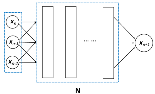
Fig. 1: Basic DNN structure for FML with $n_{M}=2$.

4 Implementation Details

In this section, we discuss the computational details to construct accurate FML models. Most of the details are associated with the use of DNNs in the FML formulation.

4.1 Multi-step loss

The long-term stability of the FML model (7) is not fully understood, largely due to our lack of understanding of the fundamental properties of DNNs. After extensive numerical experimentations, we have come to the conclusion that the stability of the FML models can be significantly enhanced by adopting a multi-step loss function during the training process.

The idea of multi-step loss is to take the averaged loss of the FML model over several time steps ahead. Let $K\geq 0$ be the number of time steps ahead. Our training data set now consists of trajectories $K$ steps longer than those in (16):

$$\left\{\mathbf{x}^{(i)}_{0},\dots,\mathbf{x}^{(i)}_{n_{M}+1},\dots,\mathbf{x}^{(i)}_{n_{M}+1+K}\right\},\qquad K\geq 0,\quad i=1,\dots,N.$$ (19)

For each of the $i$-th training trajectory, $i=1,\dots,N$, we use $\mathbf{x}_{0}^{(i)},\dots,\mathbf{x}_{n_{M}}^{(i)}$ as initial conditions and conduct the system predictions by the FML model for ($K+1$) steps:

$$\begin{split}&\widetilde{\mathbf{x}}_{0}^{(i)}=\mathbf{x}_{0}^{(i)},\quad\dots,\quad\widetilde{\mathbf{x}}_{n_{M}}^{(i)}=\mathbf{x}_{n_{M}}^{(i)},\\ &\widetilde{\mathbf{x}}_{n+1}^{(i)}=\mathbf{G}\left(\widetilde{\mathbf{x}}_{n}^{(i)},\dots,\widetilde{\mathbf{x}}_{n-n_{M}}^{(i)}\right),\qquad n=n_{M},\dots,n_{M}+K.\end{split}$$

The averaged loss against $\mathbf{x}_{n_{M}+1}^{(i)},\dots,\mathbf{x}_{n_{M}+1+K}^{(i)}$ are then computed,

$$\frac{1}{N(K+1)}\sum_{i=1}^{N}\sum_{k=0}^{K}\left\|\mathbf{x}_{n_{M}+1+k}^{(i)}-\widetilde{\mathbf{x}}_{n_{M}+1+k}^{(i)}\right\|^{2}.$$ (20)

The FML operator $\mathbf{G}$ is then computed by minimizing this multi-step loss function. It is obvious that the loss function (17) is a special case of $K=0$.

4.2 Choices of Key parameters

There are three key parameters in the FML modeling process: the time step $\Delta$, the number of memory step $n_{M}$, and the number of multi-step loss $K$.

• Time step $\Delta$. In FML modeling, the choice of the size of the time step $\Delta$ is made primarily based on the need for proper temporal resolution. In most cases, if one has the freedom to choose the time step in the raw data set (6), it is preferred to have it reasonably small to resolve the dynamics. The impact of $\Delta$ on the long-term stability of the FML prediction is not well understood. Our extensive numerical experimentation has indicated that FML models using DNNs are quite stable, when multi-step loss $K>0$ is used and the DNNs are trained with sufficient accuracy.

• Multi-step loss $K$. Using multi-step loss with $K>0$ can significantly improve the long-term numerical stability of the trained FML model. Based on our extensive numerical testing, we have found that $K=5\sim 10$ is a balanced choice. Too small a $K=1\sim 3$ results in unreliable performance for enhancing stability, whereas too big a $K>10$ does not offer any noticeable gain while significantly increasing the computational cost for DNN training.

• Memory step $n_{M}$. The choice of the memory step $n_{M}$ is perhaps the most important one. For fully observed system $\mathbf{x}=\mathbf{y}$, it is an easy choice to set $n_{M}=0$. For partially observed system $\mathbf{x}\subset\mathbf{y}$, the choice is less obvious, as it depends on the effective memory $T_{M}$ of the system in terms of $T_{M}=n_{M}\Delta$. To determine $n_{M}$ or, equivalently, $T_{M}$, we adopt a “resolution independence” procedure. That is, we start with a small $n_{M}$, and train several FML models using progressively larger $n_{M}$. Upon comparing the long-term predictions of the models, we stop the procedure when the FML model predictions start to converge. The corresponding $n_{M}$ and $T_{M}$ are then determined. It is important to recognize that although a large $T_{M}$ is always preferred mathematically, as indicated by the derivation in [6], using too large a $T_{M}$ not only makes the FML modeling computational expensive, it also induces numerical instability for the trained FML model. This is due to error accumulation of the terms in the “far back” of the memory. Those terms should have (almost) zero memory effect but numerically they are never zero due to training errors.

4.3 Training Data Generation

Once the number of memory steps $n_{M}$ and multi-step loss $K$ are determined, the total number of data entries required to compute the loss function (20) is

$$n_{data}=n_{M}+K+2.$$ (21)

Thus, each trajectories in the raw data set (6) needs to be sufficiently long such that $L_{i}>n_{data}$, $\forall i$. The trajectories with shorter length are then discarded. For trajectories with length longer than $n_{data}$, it is possible to choose multiple segments of $n_{data}$ consecutive data entries to form the training data set:

$$\left\{\mathbf{x}^{(i)}_{0},\dots,\mathbf{x}^{(i)}_{n_{M}},\dots,\mathbf{x}^{(i)}_{n_{M}+1+K}\right\},\qquad i=1,\dots,N.$$ (22)

Sometimes, one has the luxury to decide how to collect the original raw data set (6). It is then highly beneficial to choose the trajectories more strategically. Realizing that the FML model (7) is a function mapping $\mathbf{G}:\mathbb{R}^{d\times(n_{M}+1)}\to\mathbb{R}^{d}$, we can focus on sampling the observables $\mathbf{x}\in\mathbb{R}^{d}$. To this end, the “large number of short bursts” sampling strategy proposed in [25] is highly effective.

Let $\Omega_{X}$ be the phase space where we can interested in the dynamics of $\mathbf{x}$. Without loss of much generality, we assume it is a bounded hypercube. Specifically, $x_{i}\in[a_{i},b_{i}]$, where $b_{i}>a_{i}$, $i=1,\dots,d$, and $\mathbf{x}\in\Omega_{X}=\otimes_{i=1}^{d}[a_{i},b_{i}]\subset\mathbb{R}^{d}$. Our training data generation consists the following two steps:

• Generating raw data set (6). We first generate $\widetilde{N}$ trajectory data in (6). For notational simplicity, let each trajectory of the same length, i.e., $L\equiv L_{i},$ $i=1,\dots,\widetilde{N}$. We first sample $\widetilde{N}$ “initial conditions” $\mathbf{x}_{0}^{(i)}$, $i=1,\dots,\widetilde{N}$, in the domain $\Omega_{X}$. We advocate random sampling with a uniform distribution in $\Omega_{X}$, unless other prior knowledge of the distribution of $\mathbf{x}$ is available. For each initial condition $\mathbf{x}_{0}^{(i)}$, we then collect its subsequent state to form a length $L>n_{data}$ trajectory. In fact, we advocate the use of slightly longer $L$. Let $L=\gamma\cdot n_{data}$, with $\gamma=2\sim 10$. The use of the longer $L$ is to let the trajectory to start to converge to its true distribution in the phase space $\Omega_{X}$.

• Trajectory subsampling. With each trajectory in (6) longer than the required length in the training data set, i.e. $L>n_{data}$, we then randomly choose, with a uniform distribution, $n_{burst}\geq 1$ segments of $n_{data}$ consecutive entries to include in the training data set (22). The total number of training trajectories in (22) is $N=n_{burst}\cdot\widetilde{N}$. Note that when the raw data set (6) is given, using a larger number of $n_{burst}$ can boost the size of the training data set (22). However, since each trajectory in the raw data set (6) gives $n_{burst}$ trajectories of length $n_{data}$, they represent a group of highly clustered entries in the domain $\Omega_{X}$. This is undesirable for accurate function approximation. Therefore, we strongly advocate to keep $n_{burst}<10$, and whenever possible, use a smaller value. Ideally, when the raw data set (6) is easy to generate, we prefer to keep $n_{burst}=1$ and subsequently, $N=\widetilde{N}$.

4.4 DNN Training

For low-dimensional systems when $\mathbf{G}$ can be approximated by the standard methods such as orthogonal polynomials, there are many fewer uncertainties associated with the learned $\mathbf{G}$. However, when a DNN is used to represent $\mathbf{G}$, its learning induces much larger uncertainties due to the inherent randomness in the DNN training.

In order to obtain accurate and reproducible results, we present the following “guidelines” that are based on our extensive DNN training experience in the context of FML.

• Training loss. It is essential that the training loss decays at least 2 orders of magnitude from its value at the beginning of the training. This is usually accomplished via training over a large number of epochs. In most of our computations, the results were obtained with 10,000 to 20,000 epochs. Sometimes even more. To examine the training loss decay, log-scale plotting is also required.

• Validation loss. It is customary to use a small percentage, typically 5% to 10%, of the training data to compute validation loss. However, for FML, the goal is to achieve highest possible accuracy in the entire phase space of $\mathbf{x}$. A small number of samples by the validation set are not sufficient to give a good indication of the error distribution. Therefore, we do not advocate the use of validation set in FML training.

• Optimization and Learning rate. We have found the Adam optimizer to be sufficient in FML model training. The default learning rate of $10^{-3}$ in most DNN packages is usually too big. We suggest the use of a smaller learning rate on the order of $10^{-4}$, or cyclic training with $10^{-3}$ as the upper bound. Whenever the training loss does not decay at the early stage of the training, it is an indication that a smaller learning rate is necessary.

• Best model. Saving the best model based on training loss, not validation loss, is important.

• Ensemble averaging. This is perhaps the most effective way to enhance reproducibility of the FML models ([3]). With everything else fixed, we vary the initial random seeds of the optimizer and train $N_{model}>1$ DNN models independently. This in turns gives $N_{model}$ independent FML predictive models. During system prediction, each model starts with the same initial conditions and marchs forward one time step. The results are then averaged and served as the same new initial conditions to all the models in the next time step. (Note this is fundamentally different from averaging the long-term predictions of all models.) We have found that $N_{model}=5\sim 10$ is highly effective to reduce the prediction randomness in practice. Details and derivation of ensemble averaging can be found in [3].

5 Numerical Benchmarks

In this section, we present a set of well defined benchmark problems for modeling unknown dynamical systems. The problems include small linear systems, nonlinear chaotic systems, as well as a larger linear system. Both fully observed and partially observed cases are considered. To summarize, the key parameters reported in each example include

• $\Delta$: time step.

• $\Omega_{X}$: domain for initial condition sampling.

• $\widetilde{N}$: number of trajectories in the raw data set (6).

• $L$: length of the trajectories in (6).

• $N_{burst}$: number of training data trajectories taken from each raw data trajectories.

• $N$: total number of training trajectories in the training data set (22): $N=n_{burst}\cdot\widetilde{N}$.

• $n_{M}$: number of memory steps.

• $K$: number of multi-step loss.

• DNN structure: number of hidden layers, number of nodes per layer.

• Learning rate and the number of epochs for DNN training.

• $n_{model}$: number of independent FML models trained for ensemble averaging.

5.1 Small decaying linear system

The first problem is a small $2\times 2$ linear system:

$$\frac{d\mathbf{y}}{dt}=\mathbf{A}\mathbf{y},\qquad\mathbf{A}=\begin{bmatrix}1&-4\\ 4&-7\end{bmatrix}.$$ (23)

The exact solution, which decays over time, is readily available to serve as the reference solution.

5.1.1 Fully observed case

The key parameters are:

• $\Delta=0.01$.

• $\Omega_{X}=[0,2]^{2}$.

• $\widetilde{N}=10^{4}$.

• $L=200$.

• $N_{burst}=5$

• $N=n_{burst}\cdot\widetilde{N}=5\times 10^{4}$.

• $n_{M}=0$

• $K=10$.

• DNN structure: 3 hidden layers with 10 nodes per layer.

• Learning rate is $10^{-4}$; number of epochs is $10^{4}$.

• $n_{model}=10$.

For validation testing, we use $10^{2}$ new initial conditions in $\Omega_{X}$. Figure 2 shows an example trajectory, and Figure 3 shows the average $\ell_{2}$ error over the 100 test trajectories.

Fig. 2: Benchmark 5.1.1: Example trajectory prediction.

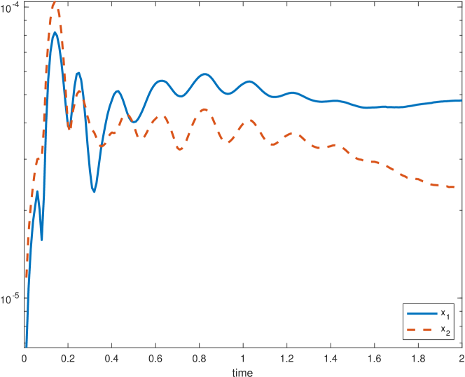
Fig. 3: Benchmark 5.1.1: Average trajectory prediction.

5.1.2 Partially observed case

We set the observable to be $x=y_{1}$. Obviously, the training data set (22) contains only the trajectory data of $y_{1}$. The memory steps, after testing, is chosen to be $n_{M}=10$. The rest of the key parameters are the same as in the previous example. The key parameters are:

• $\Delta=0.01$.

• $\Omega_{X}=[0,2]^{2}$.

• $\widetilde{N}=10^{4}$.

• $L=200$.

• $N_{burst}=5$

• $N=n_{burst}\cdot\widetilde{N}=5\times 10^{4}$.

• $n_{M}=10$

• $K=10$.

• DNN structure: 3 hidden layers with 10 nodes per layer.

• Learning rate is $10^{-4}$; number of epochs is $10^{4}$.

• $n_{model}=10$.

Figure 4 shows an example trajectory, and Figure 5 shows the average $\ell_{2}$ error over $10^{2}$ test trajectories using initial conditions uniformly sampled in $\Omega_{X}$.

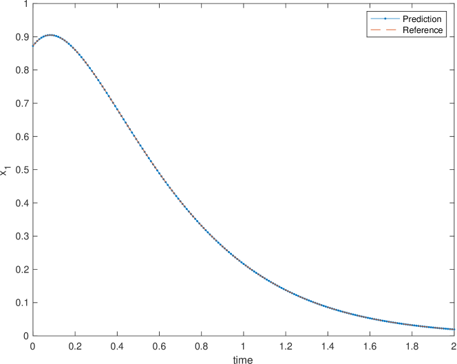
Fig. 4: Benchmark 5.1.2: Example trajectory prediction.

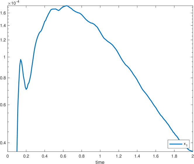
Fig. 5: Benchmark 5.1.2: Average trajectory prediction.

5.2 Oscillatory linear system

Next we consider a slightly more complex $2\times 2$ linear system:

$$\frac{d\mathbf{y}}{dt}=A\mathbf{y},\quad A=\begin{bmatrix}-\alpha^{-1}&1\\ -1&-\alpha^{-1}\end{bmatrix}\text{ with }\alpha=64.$$ (24)

Unlike the examples above, which tend to steady state monotonically after some time, the following system tends to steady state in an oscillatory manner with the size of the oscillations governed by the parameter $\alpha$.

5.2.1 Fully observed case

The key parameters are:

• $\Delta=0.01$.

• $\Omega_{X}=[0,2]^{2}$.

• $\widetilde{N}=10^{4}$.

• $L=200$.

• $N_{burst}=5$

• $N=n_{burst}\cdot\widetilde{N}=5\times 10^{4}$.

• $n_{M}=0$

• $K=10$.

• DNN structure: 3 hidden layers with 10 nodes per layer.

• Learning rate is $10^{-4}$; number of epochs is $10^{4}$.

• $n_{model}=10$.

Figure 6 shows an example trajectory, and Figure 7 shows the average $\ell_{2}$ error over $10^{2}$ test trajectories with initial conditions uniformly sampled from $\Omega_{X}$.

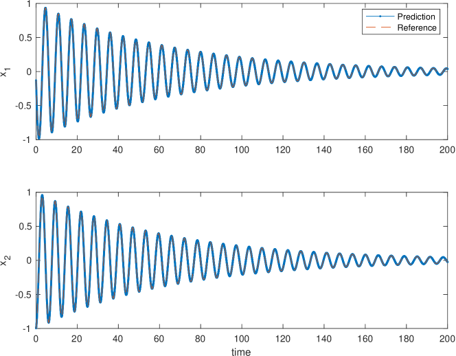
Fig. 6: Benchmark 5.2.1: Example trajectory prediction.

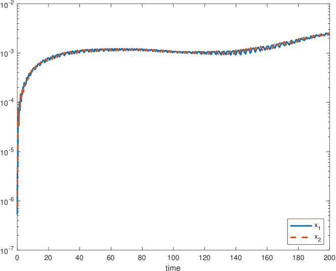
Fig. 7: Benchmark 5.2.1: Average trajectory prediction.

5.2.2 Partially observed case

We set the observable to be $x=y_{1}$. The training data set (22) therefore contains only the trajectory data of $y_{1}$. The memory step, after testing, is chosen to be $n_{M}=10$. The rest of the key parameters are the same as in the previous example:

• $\Delta=0.01$.

• $\Omega_{X}=[0,2]^{2}$.

• $\widetilde{N}=10^{4}$.

• $L=200$.

• $N_{burst}=5$

• $N=n_{burst}\cdot\widetilde{N}=5\times 10^{4}$.

• $n_{M}=10$

• $K=10$.

• DNN structure: 3 hidden layers with 10 nodes per layer.

• Learning rate is $10^{-4}$; number of epochs is $10^{4}$.

• $n_{model}=10$.

Figure 8 shows an example trajectory, and Figure 9 shows the average $\ell_{2}$ error over $10^{2}$ test trajectories with initial conditions uniformly sampled from $\Omega_{X}$.

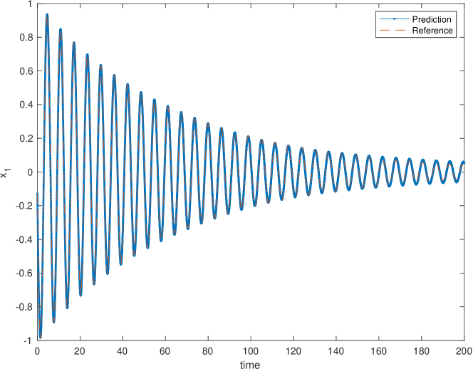
Fig. 8: Benchmark 5.2.2: Example trajectory prediction.

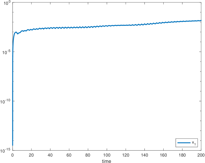
Fig. 9: Benchmark 5.2.2: Average trajectory prediction.

5.3 Oscillatory nonlinear system

The first nonlinear system we consider is a $2$-dimensional damped pendulum system:

$$\frac{dy_{1}}{dt} =y_{2}$$

$$\frac{dy_{2}}{dt} =-\alpha y_{2}-\beta\sin y_{1}$$

with $\alpha=10^{-1}$ and $\beta=9.80665$. The system exhibits oscillatory behavior as it decays to zero.

5.3.1 Fully observed case

The key parameters are:

• $\Delta=0.01$.

• $\Omega_{X}=[-\pi/2,\pi/2]\times[-\pi,\pi]$.

• $\widetilde{N}=10^{4}$.

• $L=1000$.

• $N_{burst}=5$

• $N=n_{burst}\cdot\widetilde{N}=5\times 10^{4}$.

• $n_{M}=0$

• $K=10$.

• DNN structure: 3 hidden layers with 10 nodes per layer.

• Learning rate is $10^{-4}$; number of epochs is $10^{4}$.

• $n_{model}=10$.

Figure 10 shows an example trajectory, and Figure 11 shows the average $\ell_{2}$ error over $10^{2}$ test trajectories with initial conditions uniformly sampled from $\Omega_{X}$.

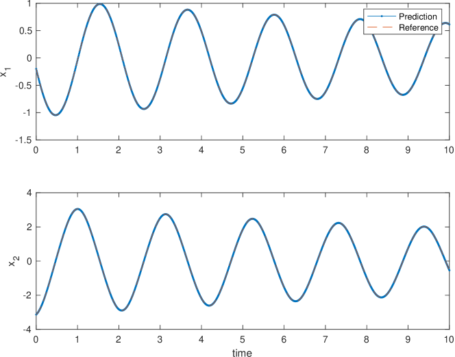
Fig. 10: Benchmark 5.3.1: Example trajectory prediction.

Fig. 11: Benchmark 5.3.1: Average trajectory prediction.

5.3.2 Fully observed case with random parameters

In the next benchmark, instead of $\alpha$ fixed we choose $\alpha$ uniformly at random from $[0,0.2]$ for each training trajectory. Note that $\alpha$ is completely unknown in the training process, and the network relies on memory step $n_{M}=10$ to learn the appropriate behavior for the entire parameter domain. The rest of the key parameters are the same as above:

• $\Delta=0.01$.

• $\Omega_{X}=[-\pi/2,\pi/2]\times[-\pi,\pi]$.

• $\widetilde{N}=10^{4}$.

• $L=1000$.

• $N_{burst}=5$

• $N=n_{burst}\cdot\widetilde{N}=5\times 10^{4}$.

• $n_{M}=10$

• $K=10$.

• DNN structure: 3 hidden layers with 10 nodes per layer.

• Learning rate is $10^{-4}$; number of epochs is $10^{4}$.

• $n_{model}=10$.

Figure 12 shows an example trajectory, and Figure 13 shows the average $\ell_{2}$ error over $10^{2}$ test trajectories with initial conditions uniformly sampled from $\Omega_{X}$.

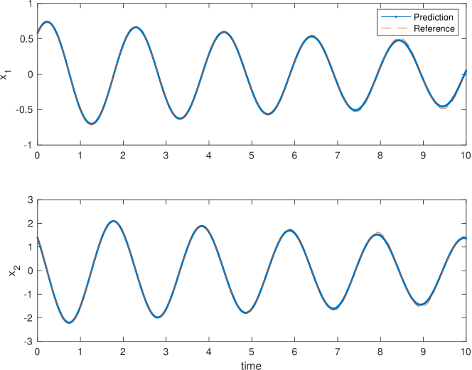
Fig. 12: Benchmark 5.3.2: Example trajectory prediction.

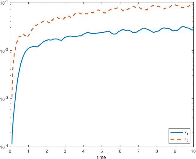
Fig. 13: Benchmark 5.3.2: Average trajectory prediction.

5.3.3 Partially observed case

Finally, we model the reduced system after observing only the first variable $x=y_{1}$. Key parameters are identical to the fully observed case with random parameters:

• $\Delta=0.01$.

• $\Omega_{X}=[-\pi/2,\pi/2]\times[-\pi,\pi]$.

• $\widetilde{N}=10^{4}$.

• $L=1000$.

• $N_{burst}=5$

• $N=n_{burst}\cdot\widetilde{N}=5\times 10^{4}$.

• $n_{M}=10$

• $K=10$.

• DNN structure: 3 hidden layers with 10 nodes per layer.

• Learning rate is $10^{-4}$; number of epochs is $10^{4}$.

• $n_{model}=10$.

Figure 14 shows an example trajectory, and Figure 15 shows the average $\ell_{2}$ error over $10^{2}$ test trajectories with initial conditions uniformly sampled from $\Omega_{X}$.

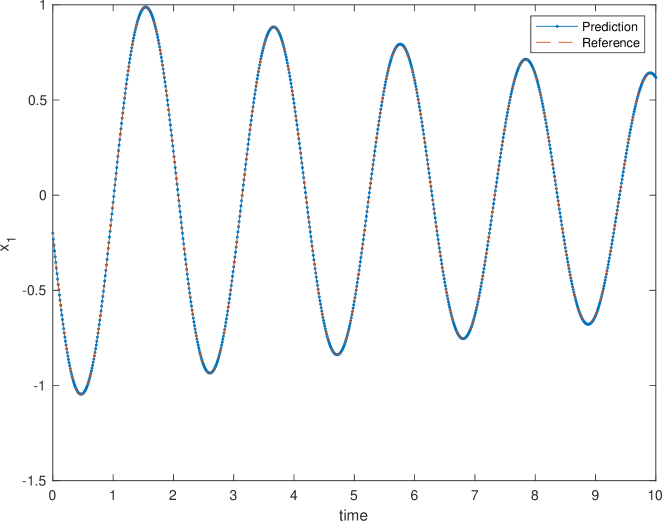
Fig. 14: Benchmark 5.3.3: Example trajectory prediction.

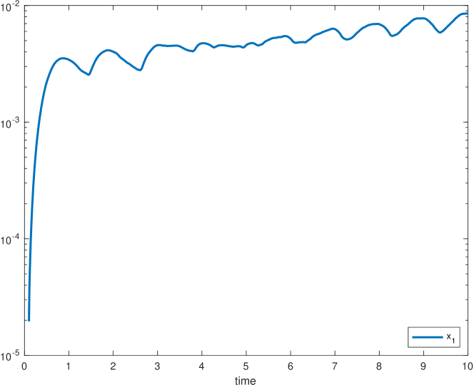
Fig. 15: Benchmark 5.3.3: Average trajectory prediction.

5.4 Chaotic nonlinear system

A typical example in learning of dynamical systems is the Lorenz ’63 system:

$$\frac{dx}{dt} =\sigma(y-x)$$

$$\frac{dy}{dt} =x(\rho-z)-y$$

$$\frac{dz}{dt} =xy-\beta z$$

with $\sigma=10$, $\rho=28$, and $\beta=8/3$. This combination of parameters causes solutions to become chaotic, arbitrarily switching between two attractors in a butterfly shape. While here we focus on three benchmarking examples for readers to reproduce, in [4] the authors more exhaustively examine flow map learning for chaotic systems and show that the proposed approach models chaotic systems well under a variety of different metrics.

5.4.1 Fully observed case

The key parameters are:

• $\Delta=0.01$.

• $\Omega_{X}=[-\pi/2,\pi/2]^{3}$.

• $\widetilde{N}=10^{4}$.

• $L=10,000$.

• $N_{burst}=5$

• $N=n_{burst}\cdot\widetilde{N}=5\times 10^{4}$.

• $n_{M}=0$

• $K=10$.

• DNN structure: 3 hidden layers with 30 nodes per layer.

• Learning rate is $10^{-4}$; number of epochs is $10^{4}$.

• $n_{model}=10$.

We note that using long training trajectories (large $L$) makes it more likely to select bursts from a time period when the system has fully settled into its chaotic behavior.

Figure 16 shows an example trajectory, and Figure 17 shows the average $\ell_{2}$ error over $10^{2}$ test trajectories with initial conditions uniformly sampled from $\Omega_{X}$.

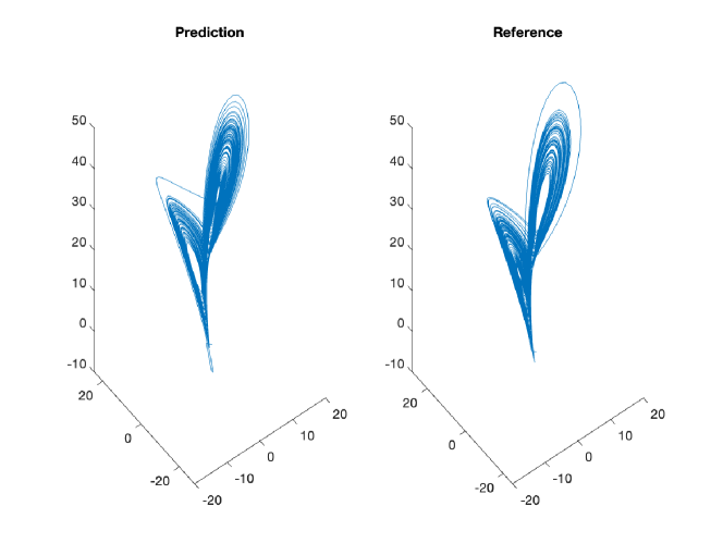
Fig. 16: Benchmark 5.4.1: Example trajectory prediction.

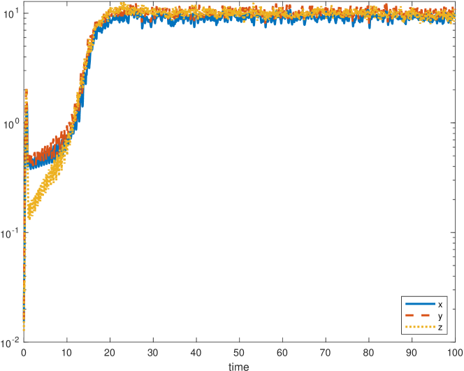
Fig. 17: Benchmark 5.4.1: Average trajectory prediction.

5.4.2 Partially observed case of $x$ and $y$

As another benchmark, we observe the $x$ and $y$ variables and let $z$ be unobserved. The key parameters are:

• $\Delta=0.01$.

• $\Omega_{X}=[-\pi/2,\pi/2]^{3}$.

• $\widetilde{N}=10^{4}$.

• $L=10,000$.

• $N_{burst}=5$

• $N=n_{burst}\cdot\widetilde{N}=5\times 10^{4}$.

• $n_{M}=10$

• $K=10$.

• DNN structure: 3 hidden layers with 30 nodes per layer.

• Learning rate is $10^{-4}$; number of epochs is $10^{4}$.

• $n_{model}=10$.

Figure 18 shows an example trajectory, and Figure 19 shows the average $\ell_{2}$ error over $10^{2}$ test trajectories with initial conditions uniformly sampled from $\Omega_{X}$.

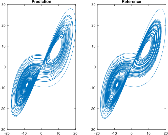
Fig. 18: Benchmark 5.4.2: Example trajectory prediction.

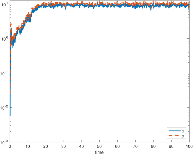
Fig. 19: Benchmark 5.4.2: Average trajectory prediction.

5.4.3 Partially observed case of $x$ only

Finally, we consider observing only $x$ and leaving $y$ and $z$ unobserved. The key parameters are:

• $\Delta=0.01$.

• $\Omega_{X}=[-\pi/2,\pi/2]^{3}$.

• $\widetilde{N}=10^{4}$.

• $L=10,000$.

• $N_{burst}=5$

• $N=n_{burst}\cdot\widetilde{N}=5\times 10^{4}$.

• $n_{M}=10$

• $K=10$.

• DNN structure: 3 hidden layers with 30 nodes per layer.

• Learning rate is $10^{-4}$; number of epochs is $10^{4}$.

• $n_{model}=10$.

Figure 20 shows an example trajectory, and Figure 21 shows the average $\ell_{2}$ error over $10^{2}$ test trajectories with initial conditions uniformly sampled from $\Omega_{X}$.

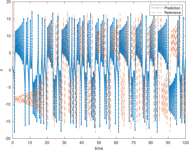
Fig. 20: Benchmark 5.4.3: Example trajectory prediction.

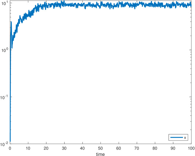
Fig. 21: Benchmark 5.4.3: Average trajectory prediction.

5.5 Large linear system

The final benchmark is a larger $20\times 20$ linear system:

$$\frac{d\mathbf{y}}{dt}=A\mathbf{y},\quad A=\begin{bmatrix}\Sigma_{11}&I+\Sigma_{12}\\ -(I+\Sigma_{21})&-\Sigma_{22}\end{bmatrix},$$ (25)

where $I$ is the $10\times 10$ identity matrix, and the fixed constant $\Sigma$ matrices are given in the Appendix.

5.5.1 Partially observed case

We model the reduced system after observing only the first $10$ variables $y_{1},\ldots,y_{10}$. The key parameters are:

• $\Delta=0.02$.

• $\Omega_{X}=[-2,2]^{20}$.

• $\widetilde{N}=10^{4}$.

• $L=100$.

• $N_{burst}=5$

• $N=n_{burst}\cdot\widetilde{N}=5\times 10^{4}$.

• $n_{M}=30$

• $K=10$.

• DNN structure: 3 hidden layers with 100 nodes per layer.

• Learning rate is $10^{-4}$; number of epochs is $10^{4}$.

• $n_{model}=10$.

Figure 22 shows an example trajectory, and Figure 23 shows the average $\ell_{2}$ error over $10^{2}$ test trajectories with initial conditions uniformly sampled from $\Omega_{X}$.

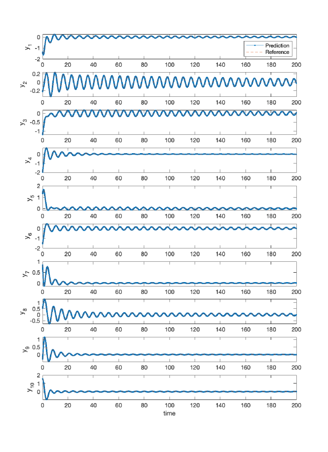
Fig. 22: Benchmark 5.5.1: Example trajectory prediction.

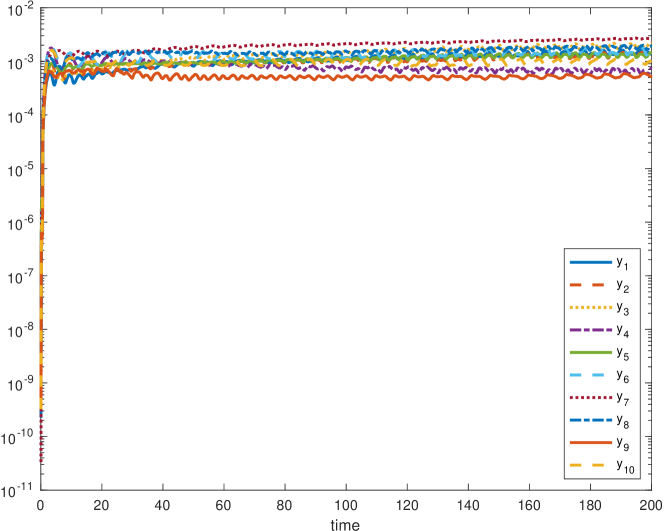
Fig. 23: Benchmark 5.5.1: Average trajectory prediction.

6 Appendix

$$\Sigma_{11}=10^{-3}\times\begin{bmatrix}-6.09&5.79&-0.945&-12.1&9.38&-12.4&4.92&3.71&1.17&4.73\\ -9.57&-8.88&-12.1&-12.9&5.11&26.5&-7.33&-8.01&-21.6&-10.2\\ -0.733&6.2&10.7&-6.06&-7.07&-1.7&-16.4&6.69&-1.59&7.69\\ 7.83&12.5&5.77&-14.9&-17.8&-1.01&-4.05&-15&-6.61&-4.94\\ 8.1&4.13&4.21&23.3&-4.63&1.77&-14.9&17.9&-17.1&-8.19\\ -7.68&6.98&27.6&19&20.9&12.2&15.6&-11.2&-3.56&-2.47\\ -14.9&-5.73&-19.7&-8.77&-9.17&-2.95&-9.48&-2.95&5.43&15.4\\ -1.84&2.05&-1.98&3.83&-4.06&7.72&4.04&-13.7&20.3&0.509\\ 12.1&19.7&-14.3&12.6&-4.67&9.72&5.87&0.664&-10.8&-18.2\\ 3.07&3.65&3.88&7.44&12.7&13.5&-6.66&-23.9&-11.7&16.6\end{bmatrix}$$ (26)

$$\Sigma_{12}=10^{-3}\times\begin{bmatrix}11.7&-12.3&-8.87&-6.86&-9.6&11&25.6&-0.155&17.8&-10.9\\ 12.9&3.28&2.84&3.35&16.6&5.96&6.99&-20.2&8.37&-8.87\\ -0.154&-16.5&12.1&0.381&11.2&-2.59&12.8&3.32&-10.9&-3.81\\ 6.49&15.8&-0.273&9.05&-3.15&0.976&-7.35&0.889&6.41&15.6\\ 4.86&-1.52&0.118&17.8&-5.08&-4.96&-2.89&3&22.4&16.4\\ 7.83&-9.66&-2.09&5.97&3.97&19.2&4.03&-15.3&-8.5&-15.8\\ -4.61&-4.98&17&-14&-17.5&0.104&-27.5&10.9&-17.9&-5.9\\ 3.88&14&-2.63&-7.27&-21&-0.403&-2.18&-22&2.01&-2.45\\ 14.4&-4.65&-8.67&-23.2&-2.73&9.58&-13.9&0.415&10.3&17.5\\ -16.8&8.18&-12.3&14.2&-18.4&-10.2&-11.4&-1.99&-2.65&-2.34\end{bmatrix}$$ (27)

$$\Sigma_{21}=10^{-3}\times\begin{bmatrix}-3.51&-4.91&-4.51&-15.8&-12&-5.72&-9.52&-14.3&0.745&-11.8\\ 1.8&2.07&8.78&5.3&-5.25&5.7&0.0957&9.77&2.17&12.8\\ -9.87&5.19&0.884&2.59&-7.95&5.56&6.41&16.4&15.6&14.3\\ 10.4&7.14&15.5&-6.6&5.33&-3.37&2.8&-9.61&8&-16.8\\ 15.5&19.6&-1.1&0.6&8.38&7.62&3.43&1.28&10.3&-4.76\\ 0.119&-9.43&-6.6&-9.99&-10.5&17.8&13.5&-6.63&-0.566&-1.81\\ -6.77&-1.42&7.46&3.32&11.7&1.3&-6.21&6.9&3.89&18.9\\ 2.93&15.1&-4.65&11.1&9.13&-9.58&-7.04&6.88&-4.07&10.2\\ -6.02&14&-5.91&-4.92&0.851&0.652&-2.57&0.835&-5.14&10.6\\ 1.41&5.8&-2.31&6.17&13.3&3.57&15.9&-0.753&-0.818&-10.3\end{bmatrix}$$ (28)

$$\Sigma_{22}=10^{-3}\times\begin{bmatrix}1500&124&814&-104&-179&-223&-731&-189&-400&242\\ 124&836&679&277&197&-515&-52.1&-273&101&301\\ 814&679&1500&651&755&-605&-379&-546&-225&223\\ -104&277&651&1960&720&-782&-299&-775&-180&506\\ -179&197&755&720&2290&-973&518&-19.1&-604&-369\\ -223&-515&-605&-782&-973&1290&-400&412&314&-420\\ -731&-52.1&-379&-299&518&-400&1960&68.3&455&-316\\ -189&-273&-546&-775&-19.1&412&68.3&576&-53.6&-332\\ -400&101&-225&-180&-604&314&455&-53.6&1030&265\\ 242&301&223&506&-369&-420&-316&-332&265&1090\end{bmatrix}$$ (29)

References

- [1] J. Bongard and H. Lipson, Automated reverse engineering of nonlinear dynamical systems, Proc. Natl. Acad. Sci., 104 (2007), pp. 9943–9948.
- [2] S. L. Brunton, J. L. Proctor, and J. N. Kutz, Discovering governing equations from data by sparse identification of nonlinear dynamical systems, Proc. Natl. Acad. Sci., 113 (2016), pp. 3932–3937.
- [3] V. Churchill, S. Manns, Z. Chen, and D. Xiu, Robust modeling of unknown dynamical systems via ensemble averaged learning, J. Comput. Phys., 474 (2023), p. 111842.
- [4] V. Churchill and D. Xiu, Deep learning of chaotic systems from partially-observed data, Journal of Machine Learning for Modeling and Computing, 3 (2022).
- [5] W. E and B. Engquist, Heterogeneous multiscale methods, Comm. Math. Sci., 1 (2003), pp. 87–132.
- [6] X. Fu, L.-B. Chang, and D. Xiu, Learning reduced systems via deep neural networks with memory, Journal of Machine Learning for Modeling and Computing, 1 (2020), pp. 97–118.
- [7] I. G. Kevrekidis, C. W. Gear, J. M. Hyman, P. G. Kevrekidid, O. Runborg, C. Theodoropoulos, et al., Equation-free, coarse-grained multiscale computation: Enabling mocroscopic simulators to perform system-level analysis, Commun. Math. Sci., 1 (2003), pp. 715–762.
- [8] J. Kutz, S. Brunton, B. Brunton, and J. Proctor, Dynamic mode decomposition: data-driven modeling of complex systems, SIAM, 2016.
- [9] Z. Long, Y. Lu, and B. Dong, PDE-Net 2.0: Learning PDEs from data with a numeric-symbolic hybrid deep network, arXiv preprint arXiv:1812.04426, (2018).
- [10] Z. Long, Y. Lu, X. Ma, and B. Dong, PDE-net: Learning PDEs from data, in Proceedings of the 35th International Conference on Machine Learning, J. Dy and A. Krause, eds., vol. 80 of Proceedings of Machine Learning Research, Stockholmsmässan, Stockholm Sweden, 10–15 Jul 2018, PMLR, pp. 3208–3216.
- [11] H. Mori, Transport, collective motion, and brownian motion, Progress of theoretical physics, 33 (1965), pp. 423–455.
- [12] T. Qin, Z. Chen, J. Jakeman, and D. Xiu, Data-driven learning of nonautonomous systems, SIAM J. Sci. Comput., 43 (2021), pp. A1607–A1624.
- [13] T. Qin, Z. Chen, J. Jakeman, and D. Xiu, Deep learning of parameterized equations with applications to uncertainty quantification, Inter. J. Uncertainty Quantification, 11 (2021), pp. 63–82.
- [14] T. Qin, K. Wu, and D. Xiu, Data driven governing equations approximation using deep neural networks, J. Comput. Phys., 395 (2019), pp. 620 – 635.
- [15] M. Raissi, Deep hidden physics models: Deep learning of nonlinear partial differential equations, Journal of Machine Learning Research, 19 (2018), pp. 1–24.
- [16] M. Raissi, P. Perdikaris, and G. E. Karniadakis, Machine learning of linear differential equations using gaussian processes, J. Comput. Phys., 348 (2017), pp. 683–693.
- [17] M. Raissi, P. Perdikaris, and G. E. Karniadakis, Physics informed deep learning (part i): Data-driven solutions of nonlinear partial differential equations, arXiv preprint arXiv:1711.10561, (2017).
- [18] M. Raissi, P. Perdikaris, and G. E. Karniadakis, Physics informed deep learning (part ii): Data-driven discovery of nonlinear partial differential equations, arXiv preprint arXiv:1711.10566, (2017).
- [19] M. Raissi, P. Perdikaris, and G. E. Karniadakis, Multistep neural networks for data-driven discovery of nonlinear dynamical systems, arXiv preprint arXiv:1801.01236, (2018).
- [20] S. H. Rudy, S. L. Brunton, J. L. Proctor, and J. N. Kutz, Data-driven discovery of partial differential equations, Science Advances, 3 (2017), p. e1602614.
- [21] S. H. Rudy, J. N. Kutz, and S. L. Brunton, Deep learning of dynamics and signal-noise decomposition with time-stepping constraints, J. Comput. Phys., 396 (2019), pp. 483–506.
- [22] H. Schaeffer, G. Tran, and R. Ward, Extracting sparse high-dimensional dynamics from limited data, SIAM Journal on Applied Mathematics, 78 (2018), pp. 3279–3295.
- [23] M. Schmidt and H. Lipson, Distilling free-form natural laws from experimental data, Science, 324 (2009), pp. 81–85.
- [24] Y. Sun, L. Zhang, and H. Schaeffer, NeuPDE: Neural network based ordinary and partial differential equations for modeling time-dependent data, arXiv preprint arXiv:1908.03190, (2019).
- [25] K. Wu and D. Xiu, Numerical aspects for approximating governing equations using data, J. Comput. Phys., 384 (2019), pp. 200–221.
- [26] R. Zwanzig, Nonlinear generalized langevin equations, Journal of Statistical Physics, 9 (1973), pp. 215–220.