Private Federated Learning with Autotuned Compression

Abstract

We propose new techniques for reducing communication in private federated learning without the need for setting or tuning compression rates. Our on-the-fly methods automatically adjust the compression rate based on the error induced during training, while maintaining provable privacy guarantees through the use of secure aggregation and differential privacy. Our techniques are provably instance-optimal for mean estimation, meaning that they can adapt to the “hardness of the problem” with minimal interactivity. We demonstrate the effectiveness of our approach on real-world datasets by achieving favorable compression rates without the need for tuning.

1 Introduction

Federated Learning (FL) is a form of distributed learning whereby a shared global model is trained collaboratively by many clients under the coordination of a central service provider. Often, clients are entities like mobile devices which may contain sensitive or personal user data. FL has a favorable construction for privacy-preserving machine learning, since user data never leaves the device. Building on top of this can provide strong trust models with rigorous user-level differential privacy (DP) guarantees Dwork et al. (2010a), which has been studied extensively in the literature Dwork et al. (2010b); McMahan et al. (2017b, 2022); Kairouz et al. (2021b).

More recently, it has become evident that secure aggregation (SecAgg) techniques Bonawitz et al. (2016); Bell et al. (2020) are required to prevent honest-but-curious servers from breaching user privacy Fowl et al. (2022); Hatamizadeh et al. (2022); Suliman and Leith (2022). Indeed, SecAgg and DP give a strong trust model for privacy-preserving FL Kairouz et al. (2021a); Chen et al. (2022a); Agarwal et al. (2021); Chen et al. (2022b); Xu et al. (2023). However, SecAgg can introduce significant communication burdens, especially in the large cohort setting which is preferred for DP. In the extreme, this can significantly limit the scalability of DP-FL with SecAgg. This motivated the study of privacy-utility-communication tradeoffs by Chen et al. (2022a), where they found that significant communication reductions could be attained essentially “for free” (see Figure 1) by using a variant of the Count Sketch linear data structure.

However, the approach of Chen et al. (2022a) suffers from a major drawback: it is unclear how to set the sketch size (i.e., compression rate) a priori. Indeed, using a small sketch may lead to a steep degradation in utility whereas a large sketch may hurt bandwidth. Further, as demonstrated in Figure 1, the “optimal” compression rate can differ substantially for different datasets, tasks, model architectures, and noise multipliers (altogether, DP configurations). This motivates the following question which we tackle in this paper:

Can we devise adaptive (autotuning) compression techniques which can find favorable compression rates in an instance-specific manner?

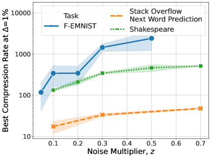
Figure 1: The optimal compression rates differ highly between different tasks. For each noise multiplier, we run compression rates of $2^{i}$, for $i\in[1,13]$, and report the highest compression rate with a maximum of $\Delta=1\%$ relative drop in accuracy from the same model without compression. We interpolate accuracies for fine-grained results. See Section 5 for task descriptions.

Naive approaches to tuning the compression rate.

Before introducing our proposed approaches, we discuss the challenges of using approaches based on standard hyper-parameter tuning. The two most common approaches are:

1. Grid-search (“Genie”): Here, we a priori fix a set of compression rates, try all of them and choose the one which has the best compression-utility (accuracy) trade-off. The problem is that this requires trying most or all compression rates, and would likely lead to even more communication in totality.

2. Doubling-trick: This involves starting with an initial optimistic guess for the compression rate, using it, and evaluating the utility for this choice. The process is then repeated, with the compression rate halved each time, until a predetermined stopping criterion is met. While this method ensures that the required communication is no more than twice the optimal amount, it can be difficult to determine a principled stopping criterion (see Figure 1 where we show that optimal compression rates depend on the task and model used). It may be desirable to maintain a high level of utility close to that of the uncompressed approach, but this requires knowledge of the utility of the uncompressed method, which is unavailable.

In our approach, instead of treating the optimization procedure as a closed-box that takes the compression rate as input, we open it up to identify the core component, mean estimation, which is more amenable to adaptive tuning.

The proxy of mean estimation.

A core component of first-order optimization methods is estimating the mean of gradients at every step. From an algorithmic perspective, this mean-estimation view has been fruitful in incorporating modern constraints, such as privacy Bassily et al. (2014); Abadi et al. (2016); Choquette-Choo et al. (2022), robustness Diakonikolas et al. (2019); Prasad et al. (2018) and compression Alistarh et al. (2017); Chen et al. (2022a); Suresh et al. (2022), by simply designing appropriate mean estimation procedures, while reusing the rest of the optimization method as is. In FL, the popular Federated Averaging (FedAvg) algorithm McMahan et al. (2017a), which we will use, computes a mean of client updates at every round.

Our theoretical results.

Previously, Chen et al. (2022a) studied federated mean estimation under the constraints of SecAgg and $(\epsilon,\delta)$-DP, and showed that with $n$ clients (data points) in $d$ dimensions, the optimal (worst-case) communication cost is $\min\left({d,n^{2}\epsilon^{2}}\right)$ bits such that the mean squared error is of the same order as optimal error under (central) DP, without any compression or SecAgg. However, in practice, the instances are rarely worst-case, and one would desire a method with more instance-specific performance. Towards this, we introduce two fine-grained descriptions of instance classes, parameterized by the (a) norm of mean (Section 3.1), which is motivated by the fact that in FL, the mean vector is the average per-round gradient and from classical optimization wisdom, its norm goes down as training progresses, and (b) tail-norm of mean (Section 3.2), which captures the setting where the mean is approximately sparse, motivated by empirical observations of this phenomena on gradients in deep learning Micikevicius et al. (2017); Shi et al. (2019).

For both of these settings, we design adaptive procedures which are oblivious to the values of norm and tail-norm, yet yield performance competitive to a method with complete knowledge of these. Specifically, for the norm of mean setting, our proposed procedure has a per-client communication complexity of roughly $\tilde{O}(n^{2}\epsilon^{2}M^{2})$ bits where $M\leq 1$ is the ratio of norm of mean to the worst-case norm bound on data points. For the tail-norm setting, we get an improved communication complexity given by the generalized sparsity of the mean – see Section 3.2 for details. Further, for both settings, we show that our proposed procedures achieve (a) optimal error under DP, without communication constraints, and (b) optimal communication complexity, under the SecAgg constraint, up to poly-logarithmic factors.

We note that adaptivity to tail-norm implies adaptivity to norm, but this comes at a price of $\operatorname{log}\left(d\right)$, rather than two, rounds of communication, which may be less favorable, especially in FL settings. We also show that interaction is necessary for achieving (nearly) optimal communication complexity, adaptively.

Finally, even without the need for adaptivity, e.g. in centralized settings, as by-products, our results yield optimal rates for DP mean estimation for the above fine-grained instance classes, parameterized by norm or tail-norm of mean, which could be of independent interest.

Our techniques.

Our compression technique, count-median-of-means sketching, is based on linear sketching, and generalizes the count-mean sketch used in Chen et al. (2022a). Our proposed protocol for federated mean estimation (FME) comprises of multiple rounds of communication in which each participating client sends two (as opposed to one) sketches. The first sketch is used to estimate the mean, as in prior work, whereas the second sketch, which is much smaller, is used to track certain statistics for adaptivity. The unifying guiding principle behind all the proposed methods is to set compression rate such that the total compression error does not overwhelm the DP error.

Experimental evaluation.

We map our mean estimation technique to the FedAvg algorithm and test it on three standard FL benchmark tasks: character/digit recognition task on the F-EMNIST dataset and next word prediction on Shakespeare and Stackoverflow datasets (see Section 5 for details). We find that our proposed technique can obtain favorable compression rates without tuning. In particular, we find that our one-shot approach tracks the potentially unachievable Genie baseline (shown in Figure 1), with no harm to model utility beyond a small slack ($\Delta\approx 1\%$) which we allow for any compression method, including the Genie. Our code is at: https://github.com/google-research/federated/tree/master/private_adaptive_linear_compression.

Related work.

Mean estimation is one of most widely studied problems in the DP literature. A standard setting deals with bounded data points Steinke and Ullman (2015); Kamath and Ullman (2020), which is what we focus on in our work. However, mean estimation has also been studied under probabilistic assumptions on the data generating process Karwa and Vadhan (2017); Bun and Steinke (2019); Kamath et al. (2020); Biswas et al. (2020); Liu et al. (2021, 2022). The work most related to ours is that of Chen et al. (2022a), which showed that in the worst-case, $O(\min(d,n^{2}\epsilon^{2}))$ bits of per-client communication is sufficient and necessary for achieving optimal error rate for SecAgg-compatible distributed DP mean estimation. Besides this, Agarwal et al. (2018, 2021); Kairouz et al. (2021a) also study compression under DP in FL settings, but rely on quantization and thus incur $\Omega(d)$ per-client communication. Finally, many works, such as Feldman and Talwar (2021); Chen et al. (2020); Asi et al. (2022); Duchi et al. (2018); Girgis et al. (2021), study mean estimation, with and without compression, under local DP Warner (1965); Kasiviswanathan et al. (2011). However, we focus on SecAgg-compatible (distributed) DP.

There has been a significant amount of research on optimization with compression in distributed and federated settings. The most common compression techniques are quantization Alistarh et al. (2017); Wen et al. (2017) and sparsification Aji and Heafield (2017); Stich et al. (2018). Moreover, the works of Makarenko et al. (2022); Jhunjhunwala et al. (2021); Chen et al. (2018) consider adaptive compression wherein the compression rate is adjusted across rounds. However, the compression techniques used in the aforementioned works are non-linear, and thus are not SecAgg compatible. The compression techniques most related to ours are of Ivkin et al. (2019); Rothchild et al. (2020); Haddadpour et al. (2020) using linear sketching. However, they do not consider adaptive compression or privacy. Finally, the works of Arora et al. (2022, 2023); Bu et al. (2021) use random projections akin to sketching in DP optimization, but in a centralized setting, for improved utility or run-time.

Organization.

We consider two tasks, Federated Mean Estimation (FME) and Federated Optimization (FO). The former primarily serves as a subroutine for the latter by considering the vector $z$ at a client to be the model update at that round of FedAvg. In Section 3, we propose two algorithms for FME : Adapt Norm, in Algorithm 1 (with the formal claim of adaptivity in Theorem 1) and Adapt Tail, in Algorithm 2 (with the formal claim of adaptivity in Theorem 3), which adapt to the norm of the mean and the tail-norm of the mean, respectively. In Section 4, we show how to extend our Adapt Norm FME protocol to the FO setting in Algorithm 3. Finally, in Section 5, we evaluate the performance of the Adapt Norm approach for FO on benchmark tasks in FL.

2 Preliminaries

Definition 1 ($(\epsilon,\delta)$-Differential Privacy).

An algorithm ${\mathcal{A}}$ satisfies $(\epsilon,\delta)$-differential privacy if for all datasets $D$ and $D^{\prime}$ differing in one data point and all events ${\mathcal{E}}$ in the range of the ${\mathcal{A}}$, we have, $\mathbb{P}\left({{\mathcal{A}}(D)\in{\mathcal{E}}}\right)\leq e^{\varepsilon}\mathbb{P}\left({{\mathcal{A}}(D^{\prime})\in{\mathcal{E}}}\right)+\delta$.

Secure Aggregation (SecAgg).

SecAgg is a cryptographic technique that allows multiple parties to compute an aggregate value, such as a sum or average, without revealing their individual contributions to the computation. In the context of FL, the works of Bonawitz et al. (2016); Bell et al. (2020) proposed practical SecAgg schemes. We assume SecAgg as default, as is the case in typical FL systems.

Count-mean sketching.

We describe the compression technique of Chen et al. (2022a), which is based on the sparse Johnson-Lindenstrauss (JL) random matrix/count-mean sketch data structure Kane and Nelson (2014). The sketching operation is a linear map, denoted as $S:{\mathbb{R}}^{d}\rightarrow{\mathbb{R}}^{PC}$, where $P,C\in{\mathbb{N}}$ are parameters. The corresponding unsketching operation is denoted as $U:{\mathbb{R}}^{PC}\rightarrow{\mathbb{R}}^{d}$. To explain the sketching operation, we begin by introducing the count-sketch data structure. A count-sketch is a linear map, which for $j\in[P]$, is denoted as $S_{j}:{\mathbb{R}}^{d}\rightarrow{\mathbb{R}}^{C}$. It is described using two hash functions: bucketing hash $h_{j}:[d]\rightarrow[C]$ and sign hash: $s_{j}:[d]\rightarrow\left\{{-1,1}\right\}$, mapping the $q$-th co-ordinate $z_{q}$ to $\sum_{i=1}^{d}s_{j}(i)\mathbbm{1}\left({h_{j}(i)=h_{j}(q)}\right)z_{i}$.

The count-mean sketch construction pads $P$ count sketches to get $S:{\mathbb{R}}^{d}\rightarrow{\mathbb{R}}^{PC}$, mapping $z$ as follows,

$$S(z)=({1}/{\sqrt{P}})\begin{bmatrix}{S_{1}}^{\top}{S_{2}}^{\top}&\cdots&{S_{P}}^{\top}\end{bmatrix}^{\top}z\;.$$

The above, being a JL matrix, approximately preserves norms of $z$ i.e. $\left\|{S(z)}\right\|\approx\left\|{z}\right\|$, which is useful in controlling sensitivity, thus enabling application of DP techniques. The unsketching operation is simply $U(S(z))=S^{\top}S(z)$. This gives an unbiased estimate, ${\mathbb{E}}[S^{T}S(z)]=z$, whose variance scales as $d\|z\|^{2}/(PC)$. This captures the trade-off between compression rate, $d/PC$, and error.

3 Instance-Optimal Federated Mean Estimation (FME)

A central operation in standard federated learning (FL) algorithms is averaging the client model updates in a distributed manner. This can be posed as a standard distributed mean estimation (DME) problem with $n$ clients, each with a vector $z_{i}\in{\mathbb{R}}^{d}$ sampled i.i.d. from an unknown distribution ${\mathcal{D}}$ with population mean $\mu$. The goal of the server is to estimate $\mu$ while communicating only a small number of bits with the clients at each round. Once we have a communication efficient scheme, this can be readily integrated into the learning algorithm of choice, such as FedAvg.

In order to provide privacy and security of the clients’ data, mean estimation for FL has additional requirements: we can only access the clients via SecAgg Bonawitz et al. (2016) and we need to satisfy DP Dwork et al. (2014). We refer to this problem as Federated Mean Estimation (FME). To bound the sensitivity of the empirical mean, $\widehat{\mu}(\{z_{i}\}_{i=1}^{n}):=(1/n)\sum_{i=1}^{n}z_{i}$, the data is assumed to be bounded by $\left\|{z_{i}}\right\|\leq G$. Since gradient norm clipping is almost always used in the DP FL setting, we assume $G$ is known. The first result characterizing the communication cost of FME is by Chen et al. (2022a), who propose an unbiased estimator based on count-mean sketching that satisfy $(\epsilon,\delta)$-differential privacy and (order) optimal error of

$$\mathbb{E}[\left\|{\overline{\mu}-\mu}\right\|^{2}]\;=\;\tilde{\Theta}\left({G^{2}\left({\frac{d}{n^{2}\epsilon^{2}}+\frac{1}{n}}\right)}\right),$$ (1)

with an (order) optimal communication complexity of $\tilde{O}(n^{2}\epsilon^{2})$. The error rate in Equation 1 is optimal as it matches the information theoretic lower bound of Steinke and Ullman (2015) that holds even without any communication constraints. The communication cost of $\tilde{O}(n^{2}\epsilon^{2})$ cannot be improved for the worst-case data as it matches the lower bound in Chen et al. (2022a). However, it might be possible to improve on communication for specific instances of $\mu$. We thus ask the fundamental question of how much communication is necessary and sufficient to achieve the optimal error rate as a function of the “hardness” of the problem.

3.1 Adapting to the Instance’s Norm

Our more fine-grained error analysis of the scheme in Chen et al. (2022a) shows that, with a sketch size of $O(PC)$ that costs $O(PC)$ in per client communication, one can achieve

$$\mathbb{E}[\left\|{\overline{\mu}-\mu}\right\|^{2}]=\tilde{O}\Big{(}G^{2}\,\Big{(}\frac{d(M^{2}+1/n)}{PC}+\frac{d}{n^{2}\epsilon^{2}}+\frac{1}{n}\Big{)}\Big{)}\,,$$ (2)

where we define the normalized norm of the mean, $M\;\;=\;\;\frac{\left\|{\mu}\right\|}{G}=\;\;\frac{\left\|{\mathbb{E}\left[z\right]}\right\|}{G}\,\in\,[0,1]\;$ and $G$ is the maximum $\lVert z\rVert$ as chosen for a sensitivity bound under DP FL. The first error term captures how the sketching error scales as the norm of the mean, $MG$. When $M$ is significantly smaller than one, as motivated by our application to FL in Section 1, a significantly smaller choice of the communication cost, $PC=O(\min\left({n^{2}\epsilon^{2},nd}\right)\left({M^{2}+1/n}\right))$, is sufficient to achieve the optimal error rate of Equation 1. The dominant term is smaller than the standard sketch size of $PC=O(n^{2}\epsilon^{2})$ by a factor of $M^{2}\in[0,1]$. However, selecting this sketch size requires knowledge of $M$. This necessitates a scheme that adapts to the current instance by privately estimating $M$ with a small communication cost. This leads to the design of our proposed interactive Algorithm 1.

Precisely, we call an FME algorithm instance-optimal with respect to $M$ if it achieves the optimal error rate of Equation 1 with communication complexity of $O(M^{2}n^{2}\epsilon^{2})$ for every instance whose norm of the mean is bounded by $GM$. We propose a novel adaptive compression scheme in Section 3.1.1 and show instance optimality in Section 3.1.2.

3.1.1 Instance-optimal FME for norm $M$

We present a two-round procedure that achieves the optimal error in Equation 1 with instance-optimal communication complexity of $O\left({\min\left({d,M^{2}n^{2}\epsilon^{2}/\operatorname{log}\left(1/\delta\right),M^{2}nd}\right)}\right)$, without prior knowledge of $M$. The main idea is to use count-mean sketch and in the first round, to construct a private yet accurate estimate of $M$. This is enabled by the fact the count-mean sketch approximately preserves norms. In the second round, we set the sketch size based on this estimate. Such interactivity is $(i)$ provably necessary for instance-optimal FME as we show in Theorem 2, and $(ii)$ needed in other problems that target instance-optimal bounds with DP Berrett and Butucea (2020).

The client protocol (line 3 in Algorithm 1) is similar to that in Chen et al. (2022a); each client computes a sketch, clips it, and sends it to the server. However, it crucially differs in that each client sends two sketches. The second sketch is used for estimating the statistic to ensure that we can achieve instance-optimal compression-utility tradeoffs as outlined in $(i)$ and $(ii)$ above. We remark that even though only one sketch is needed for the Adapt Norm approach, since the statistic can be directly estimated from the (first) sketch $S$ without a second sketch, allowing for additional minor communication optimization, we standardize our presentation on this two-sketch approach to make it inline with the Adapt Tail approach presented in Section 3.2 which requires both sketches.

Algorithm 1 Adapt Norm FME

0:  Sketch sizes $C_{1},P,\tilde{C},\tilde{P}$, noise variance $\tilde{\sigma}$, $\sigma$, $\overline{\gamma}$, client data $\left\{{z_{c}}\right\}_{c}$

1:  for $j=1$ to $2$ do

2:     Select $n$ random clients $\{z_{c}^{(j)}\}_{c=1}^{n}$ and broadcast sketching operators $S_{j}$ and $\tilde{S}$ of sizes $(C_{j},P)$ and $(\tilde{C},\tilde{P})$, respectively.

3:     SecAgg: $\nu_{j}=\!\text{SecAgg}(\{Q^{(c)}_{j}\}_{c=1}^{n})+{\mathcal{N}}\left(0,\frac{\sigma^{2}}{n}{\mathbb{I}}_{PC}\right)$, $\tilde{\nu}_{j}\!=\!\text{SecAgg}(\{\tilde{Q}^{(c)}_{j}\}_{c=1}^{n})$, where $Q^{(c)}_{j}\leftarrow\mathsf{clip}_{B}(S_{j}(z^{(j)}_{c}))$, $\tilde{Q}^{(c)}_{j}\leftarrow\mathsf{clip}_{B}(\tilde{S}_{j}(z^{(j)}_{c}))$

4:     Unsketch DP mean: Compute $\bar{\mu}_{j}=U_{j}(\nu_{j})$

5:     Estimate DP norm: $\widehat{n}_{j}\!\!=\!\text{clip}_{B}(\left\|{\tilde{\nu}_{j}}\right\|)\!+\!\text{Laplace}(\tilde{\sigma})$

6:     $C_{j+1}=\max\left({\left\lceil\min\left({\frac{n^{2}\epsilon^{2}}{\operatorname{log}\left(1/\delta\right)},nd}\right)\frac{\left({\widehat{n}_{j}+\overline{\gamma}}\right)^{2}}{G^{2}P}\right\rceil,2}\right)$

7:  end for

The server protocol, in Algorithm 1, aggregates the sketches using SecAgg (line 3). In the first round, $Q_{j}$’s are not used, i.e., $C_{1}=0$. Only $\tilde{Q}_{j}$’s are used to construct a private estimate of the norm of the mean $\widehat{n}_{1}$ (line 5). We do not need to unsketch $\tilde{Q}_{j}$’s as the norm is preserved under our sketching operation. We use this estimate to set the next round’s sketch size, $C_{j+1}$ (line 6), so as to ensure the compression error of the same order as privacy and statistical error; this is the same choice we made when we assumed oracle knowledge of $M$—see discussion after Equation 2. In the second round and onwards, we use the first sketch, which is aggregated using SecAgg and privatized by adding appropriately scaled Gaussian noise (line 3). Finally, the $Q_{j}$’s are unsketched to estimate the mean. Note that the clients need not send $\tilde{Q}_{j}$’s after the first round.

3.1.2 Theoretical analysis

We show that the Adapt Norm approach (Algorithm 1) achieves instance-optimality with respect to $M$; an optimal error rate of Equation 1 is achieved for every instance of the problem with an efficient communication complexity of $O(M^{2}n^{2}\epsilon^{2})$ (Theorem 1). The optimality follows from a matching lower bound in Corollary 1. We further establish that interactivity, which is a key feature of Algorithm 1, is critical in achieving instance-optimality. This follows from a lower bound in Theorem 2 that proves a fundamental gap between interactive and non-interactive algorithms.

Theorem 1.

For any choice of the failure probability $0<\beta<\min\left({\frac{\operatorname{log}\left(1/\delta\right)}{n^{2}\epsilon^{2}},1}\right)$, Algorithm 1 with $B=2G,C_{1}=0,P=\tilde{P}=\lceil\Theta\left({\operatorname{log}\left(4/\beta\right)}\right)\rceil,\tilde{C}=2,\sigma^{2}=\frac{256B^{2}\operatorname{log}\left(1/\delta\right)}{\epsilon^{2}},\tilde{\sigma}=\frac{4B}{n\epsilon}\text{ and }\overline{\gamma}=\frac{2B\operatorname{log}\left(8/\beta\right)}{n\epsilon}+\frac{B\sqrt{\operatorname{log}\left(16/\beta\right)}}{\sqrt{n}}$ satisfies $(\epsilon,\delta)$-DP, the output $\bar{\mu}_{2}$ is an unbiased estimate of mean, and its error is bounded as,

$$\mathbb{E}[\left\|{\bar{\mu}_{2}-\mu}\right\|]^{2}\leq O\left({G^{2}\left({\frac{d\operatorname{log}\left(1/\delta\right)}{n^{2}\epsilon^{2}}+\frac{1}{n}}\right)}\right)\;.$$

Finally, the number of rounds is two, and with probability at least $1-\beta$, the total per-client communication complexity is $\tilde{O}\left({\min\left({\frac{n^{2}\epsilon^{2}}{\operatorname{log}\left(1/\delta\right)},nd}\right)\left({M^{2}+\frac{1}{n^{2}\epsilon^{2}}+\frac{1}{n}}\right)}\right)$.

We provide a proof in Appendix C. The error rate matches Equation 1 and cannot be improved in general. Compared to the target communication complexity of $O((M^{2}+1/n)n^{2}\epsilon^{2})$, the above communication complexity has an additional term $1/(n\epsilon)^{2}$, which stems from the fact that the norm can only be accessed privately. In the interesting regime where the error is strictly less than the trivial $M^{2}G^{2}$, the extra $1/(n\epsilon)^{2}+1/n$ is smaller than $M^{2}$. The resulting communication complexity is $O(M^{2}n^{2}\epsilon^{2}/\operatorname{log}\left(1/\delta\right))$. This nearly matches the oracle communication complexity that has the knowledge of $M$. In the following, we make this precise.

Algorithm 1 is instance-optimal with respect to ${\bm{M}}$.

The next theorem shows that even under the knowledge of $M$, no unbiased procedure under a SecAgg constraint with optimal error can have smaller communication complexity than the above procedure. We provide a proof in Appendix E.

Corollary 1 (Chen et al. (2022a) Theorem 5.3).

Let $K,d,n\in{\mathbb{N}}$, $M,G,\epsilon,\delta\geq 0$, and ${\mathcal{P}}_{1}(d,G,M):=\left\{{{\mathcal{D}}\text{ over }{\mathbb{R}}^{d}:\left\|{z}\right\|\leq G\text{ for }z\sim{\mathcal{D}}\text{ and }\left\|{\mu({\mathcal{D}})}\right\|\leq MG}\right\}$. For any $K$, any $K$-round unbiased SecAgg-compatible protocol ${\mathcal{A}}$ (see Appendix E for details) such that $\mathbb{E}_{D\sim{\mathcal{D}}^{n}}[\left\|{{\mathcal{A}}(D)-\mu}\right\|^{2}]=O\left({\min\left({M^{2}G^{2},\frac{G^{2}}{n}+\frac{G^{2}d\operatorname{log}\left(1/\delta\right)}{n^{2}\epsilon^{2}}}\right)}\right)\ \forall\ {\mathcal{D}}\in{\mathcal{P}}_{1}(d,G,M)$, there exists a distribution ${\mathcal{D}}\in{\mathcal{P}}_{1}(d,G,M)$, such that on dataset $D\sim{\mathcal{D}}^{n}$, w.p. 1, the total per-client communication complexity is $\Omega\left({\min\left({d,\frac{M^{2}n^{2}\epsilon^{2}}{\operatorname{log}\left(1/\delta\right)},M^{2}nd}\right)}\right)$ bits.

Interaction is necessary.

A key feature of our algorithm is interactivity: the norm of the mean estimated in the prior round is used to determine the sketch size in the next round. We show that at least two rounds of communication are necessary for any algorithm with instance-optimal communication complexity. This proves a fundamental gap between interactive and non-interactive approaches in solving FME. We provide a proof in Appendix E.

Theorem 2.

Let $K,d,n\in{\mathbb{N}},n\geq 2$, $G,\epsilon,\delta>0$, and ${\mathcal{P}}_{2}(d,G):=\left\{{{\mathcal{D}}\text{ over }{\mathbb{R}}^{d}:\left\|{z}\right\|\leq G\text{ for }z\sim{\mathcal{D}}}\right\}$. Let ${\mathcal{A}}$ be a $K$-round unbiased SecAgg-compatible protocol with $\underset{D\sim{\mathcal{D}}^{n}}{\mathbb{E}}[\left\|{{\mathcal{A}}(D)-\mu({\mathcal{D}})}\right\|^{2}]=O\Big{(}\min\Big{(}\left\|{\mu({\mathcal{D}})}\right\|^{2},\frac{G^{2}}{n}+\frac{G^{2}d\operatorname{log}\left(1/\delta\right)}{n^{2}\epsilon^{2}}\Big{)}\Big{)}$ and total per-client communication complexity of $O\Big{(}\min\Big{(}d,\frac{\left\|{\mu({\mathcal{D}})}\right\|^{2}n^{2}\epsilon^{2}}{\operatorname{log}\left(1/\delta\right)},\left\|{\mu({\mathcal{D}})}\right\|^{2}nd\Big{)}\Big{)}$ bits with probability $>\frac{1}{n}$, point-wise $\forall\ {\mathcal{D}}\in{\mathcal{P}}_{2}(d,G)$. Then $K\geq 2$.

3.2 Adapting to the Instance’s Tail-norm

The key idea in norm-adaptive compression is interactivity. On top of interactivity, another key idea in tail-norm-adaptive compression is count median-of-means sketching.

Count median-of-means sketching.

Our new sketching technique takes $R\in{\mathbb{N}}$ independent count-mean sketches of Chen et al. (2022a) (see Section 2). Let $S^{(i)}:{\mathbb{R}}^{d}\rightarrow{\mathbb{R}}^{PC}$ denote the $i$-th count-mean sketch. Our sketching operation, $S:{\mathbb{R}}^{d}\rightarrow{\mathbb{R}}^{R\times PC}$, is defined as the concatenation: $S(z)=Sz=\begin{bmatrix}(S^{(1)}z)^{\top}(S^{(2)}z)^{\top}\ldots(S^{(R)}z)^{\top}\end{bmatrix}^{\top}$. Our median-of-means unsketching takes the median over $R$ unsketched estimates: $U(S(z))_{j}=\text{Median}(\{({S^{(i)}}^{\top}S^{(i)}z)_{j}\}_{i=1}^{R})$. This median trick boosts the confidence to get a high probability of success (as opposed to a guarantee in expectation) and to get tail-norm (as opposed to norm) based bounds Charikar et al. (2002). However, in non-private settings, it suffices to take multiple copies of a count-sketch, which in our notation, corresponds to setting $P=1$. On the other hand, we set $P>1$ to get bounded sensitivity which is useful for DP, yielding our (novel) count-median-of-means sketching technique. We remark that in some places, we augment the unsketching operation with “Top_k”, which returns top-$k$ coordinates, of a vector, in magnitude.

Algorithm 2 Adapt Tail FME

0:  Sketch sizes $R,C_{1},P,\tilde{R},\tilde{C},\tilde{P}$, noise $\sigma$, $\tilde{\sigma}$, $\left\{{{k_{j}}}\right\}_{j}$, $\left\{{\overline{\gamma}_{j}}\right\}_{j}$, rounds $K$, client data $\left\{{z_{c}}\right\}_{c}$

1:  for $j=1$ to $K$ do

2:     Select $n$ random clients $\{z_{c}^{(j)}\}_{c=1}^{n}$ and broadcast sketching operators $S_{j}$ and $\tilde{S}_{j}$ of sizes $(R,C_{j},P)$ and $(\tilde{R},\tilde{C},\tilde{P})$ respectively..

3:     SecAgg: $\nu_{j}=\!\text{SecAgg}(\{Q^{(c)}_{j}\}_{c=1}^{n})+{\mathcal{N}}\left(0,\frac{\sigma^{2}}{n}{\mathbb{I}}_{PC}\right)$, $\tilde{\nu}_{j}\!=\!\text{SecAgg}(\{\tilde{Q}^{(c)}_{j}\}_{c=1}^{n})$ , where $Q^{(c)}_{j}\!\!\leftarrow\!\![\mathsf{clip}_{B}(S^{(i)}_{j}(z^{(j)}_{c}))]_{i=1}^{R}$, $\tilde{Q}^{(c)}_{j}\!\!\leftarrow[\mathsf{clip}_{B}(\tilde{S}^{(i)}_{j}(z^{(j)}_{c}))]_{i=1}^{\tilde{R}}$

4:     Unsketch DP mean: Compute $\bar{\mu}_{j}=\text{Top}_{{k_{j}}}(U_{j}(\nu_{j}))$

5:     Estimate error: $\bar{e}_{j}=\left\|{\tilde{S}_{j}(\bar{\mu}_{j})-\tilde{\nu}_{j}}\right\|$

6:     $\tilde{\gamma}_{j}=\bar{\gamma}_{j}+\text{Laplace}(\tilde{\sigma})$ and $\tilde{e}_{j}=\bar{e}_{j}+\text{Laplace}(2\tilde{\sigma})$

7:     If $\tilde{e}_{j}\leq\tilde{\gamma}_{j}$, set $\bar{\mu}=\bar{\mu}_{j}$, break

8:     $C_{j+1}=2C_{j}$

9:  end for

Approximately-sparse setting.

We expect improved guarantees when $\mu$ is approximately sparse. This is captured by the tail-norm. Given $z\in{\mathbb{R}}^{d},\left\|{z}\right\|\leq G$, and $k\in[d]$, the normalized tail-norm is $\left\|{z_{\text{n-tail}({k})}}\right\|_{2}:=\frac{1}{G}\min_{\tilde{z}:\left\|{\tilde{z}}\right\|_{0}\leq k}\left\|{z-\tilde{z}}\right\|_{2}\;$. This measures the error in the best $k$-sparse approximation. We show that the mean estimate via count median-of-means sketch is still unbiased (Lemma 7), and for $C=\Omega\left({Pk}\right)$, has error bounded as,

$$\left\|{\bar{\mu}-\mu}\right\|_{2}^{2}\!=\!O\Big{(}\frac{dG^{2}}{PC}\Big{(}\left\|{\mu_{\text{n-tail}({k})}}\right\|^{2}+\frac{1}{n}\Big{)}+\frac{G^{2}}{n}+\frac{G^{2}d}{n^{2}\epsilon^{2}}\Big{)}$$ (3)

If all tail-norms are known, then we can set the sketch size $PC=\min_{k}\max\left({k,\min\left({nd,n^{2}\epsilon^{2}}\right)\left({\left\|{\mu_{\text{n-tail}({k})}}\right\|^{2}+\frac{1}{n}}\right)}\right)$, and achieve the error rate in Equation 1. When $k=0$, this recovers the previous communication complexity of count-mean sketch in Section 3.1. For optimal choice of $k$, this communication complexity can be smaller. We aim to achieve it adaptively, without the (unreasonable) assumption of knowledge of all the tail-norms.

3.2.1 Instance-optimal FME for tail-norm

Previously, we estimated the norm of the mean in one round. Now, we need multiple tail-norms. We propose a doubling-trick based scheme. Starting from an optimistic guess of the sketch size, we progressively double it, until an appropriate stopping criterion on the error is met. The main challenge is in estimating the error of the first sketch $S$ (for the current choice of sketch size), as naively this would require the uncompressed true vector $z$ to be sent to the server. To this end, we show how to use the second sketch $\tilde{S}$ so as to obtain a reasonable estimate of this error, while using significantly less communication than transmitting the original $z$.

We re-sketch the unsketched estimate, $U(S(z))$, of $z$ with $\tilde{S}$. The reason is that this can now be compared with the second sketch $\tilde{S}(z)$ to get an estimate of the error: $\left\|{\tilde{S}(U(S(z)))-\tilde{S}(z)}\right\|^{2}=\left\|{\tilde{S}(U(S(z))-z)}\right\|^{2}\approx\left\|{U(S(z)))-z}\right\|^{2}$, where we used the linearity and norm-preservation property of the count-sketch.

Algorithm 2 presents the pseudo-code for Adapt Tail. The client protocol remains the same; each participating client sends two independent (count median-of-mean) sketches to the server. The server, starting from an optimistic choice of initial sketch size $PC_{1}$, obtains the aggregated sketches from the clients via SecAgg and adds noise to the first sketch for DP (line 4). It then unsketches the first sketch to get an estimate of mean, $\bar{\mu}_{j}$ (line 4)—we note that $\text{Top}_{k_{j}}$ is not applied (i.e., $k_{j}=d$) for the upcoming result but will be useful later. We then sketch $\bar{\mu}_{j}$ with the second sketch $\tilde{S}$ and compute the norm of difference with the aggregated second sketch from clients (line 5)—this gives an estimate of the error of $\bar{\mu}_{j}$. Finally, we want to stop if the error is sufficiently small, dictated by the threshold $\overline{\gamma}_{j}$, which will be set as target error in Equation 1. To preserve privacy at this step, we use the well-known AboveThreshold algorithm Dwork et al. (2014), which adds noise to both the error and threshold (line 6) and stops if the noisy error is smaller than the noisy threshold (line 7). If this criterion is not met, then we double the first sketch size (line 8) and repeat.

3.2.2 Theoretical analysis

Given a non-decreasing function $g:[d]\rightarrow{\mathbb{R}}$, we define the generalized sparsity as $k_{\text{tail}}(g(k);\mu):=\min_{k\in[d]}\left\{{k:\left\|{\mu_{\text{\text{n-tail}({k})}}}\right\|^{2}\leq g(k)}\right\}$. In the special case when $g(k)\equiv 0$, this recovers the sparsity of $\mu$.

We now present our result for the proposed Adapt Tail approach.

Theorem 3.

For any choice of failure probability $0\!\!<\!\!\beta\!\!<\!\!1$, Algorithm 2 with $B\!\!\!=\!\!\!2G,{k_{j}}\!=\!d,K\!\!\!\!=\!\!\!\!\lfloor\operatorname{log}\left(d\right)\rfloor,\tilde{\sigma}\!=\!\frac{4B}{n\epsilon},\sigma^{2}\!=\!\frac{256R\left({\operatorname{log}\left(d\right)}\right)^{2}B^{2}\operatorname{log}\left(1/\delta\right)}{\epsilon^{2}},R\!\!\!\!=\!\!\!\!\left\lceil 2\operatorname{log}\left(8d\operatorname{log}\left(d\right)/\beta\right)\right\rceil,C_{1}\!\!\!=\!\!\!8P,P\!\!\!\!\!\!=\!\!\!\!\!\!\lceil\Theta(2\operatorname{log}\left(8R\operatorname{log}\left(d\right)/\beta\right))\rceil,\tilde{C}\!\!\!\!\!=\!\!\!\!\!2\tilde{P},\tilde{R}\!\!\!\!\!\!=\!\!\!\!\!\!\!1,\tilde{P}\!\!=\!\!\lceil\Theta\left({2\operatorname{log}\left(4d\operatorname{log}\left(d\right)/\beta\right)}\right)\rceil,\overline{\gamma}_{j}=\overline{\gamma}=15\max\left({\frac{G\sqrt{\operatorname{log}\left(8\operatorname{log}\left(d\right)/\beta\right)}}{\sqrt{n}},\sqrt{d}\frac{\sigma}{n}}\right)+\tilde{\alpha}\qquad\text{and }\tilde{\alpha}=\frac{32B\left({\operatorname{log}\left(\lfloor\operatorname{log}\left(d\right)\rfloor\right)+\operatorname{log}\left(8/\beta\right)}\right)}{n\epsilon},$ satisfies $(\epsilon,\delta)$-DP, and outputs an unbiased estimate of the mean. With probability at least $1-\beta$, the error is bounded as,

$$\left\|{\bar{\mu}-\mu}\right\|^{2}=\tilde{O}\left({\frac{G^{2}}{n}+\frac{G^{2}d\operatorname{log}\left(1/\delta\right)}{n^{2}\epsilon^{2}}}\right),$$

the total per-client communication complexity is $\tilde{O}\left({k_{\text{tail}}(g(k));\mu)}\right)$, where $g(k)=\max\left({\frac{1}{nd},\frac{\operatorname{log}\left(1/\delta\right)}{n^{2}\epsilon^{2}}}\right)k-\frac{4\operatorname{log}\left(8\operatorname{log}\left(d\right)/\beta\right)}{n}$, and number of rounds is $\lfloor\operatorname{log}\left(d\right)\rfloor$.

We provide the proof of Theorem 3 in Appendix C. First, we argue that the communication complexity is of the same order as of this method with prior knowledge of all tail norms—plugging in $g(k)$ in the definition of $k_{\text{tail}}(g(k);\mu)$ gives us that $k_{\text{tail}}(g(k);\mu)$ is the smallest $k$ such that $k\geq\min\left({nd,n^{2}\epsilon^{2}}\right)\left({\left\|{\mu_{\text{n-tail}({k})}}\right\|^{2}+\frac{1}{n}}\right)$. This is what we obtained before, which further is no larger than the result on adapting to norm of mean (Theorem 1)—see discussion after Equation 3. However, this algorithm requires $\lfloor\operatorname{log}\left(d\right)\rfloor$ rounds of interaction, as opposed to two in Theorem 1. It therefore depends on the use-case which of the two, total communication or number of rounds, is more important.

The error rate in Theorem 3 matches that in Equation 1, known to be optimal in the worst case. However, it may be possible to do better for specific values of tail-norms. Under the setting where the algorithm designer is given $k<d$ and $\gamma$ and is promised that $\left\|{\mu_{\text{n-tail}({k})}}\right\|\leq\gamma$, we give a lower bound of $\Omega\left({G^{2}\min\left\{{1,\gamma^{2}+\frac{k}{n^{2}\epsilon^{2}}+\frac{1}{n},\frac{d}{n^{2}\epsilon^{2}}+\frac{1}{n}}\right\}}\right)$ on error of (central) DP mean estimation (see Theorem 5). The second term here is new, and we show that a simple tweak to our procedure underlying Theorem 3—adding a Top_k operation, with exponentially increasing $k$, to the unsketched estimate—suffices to achieve this error (see Theorem 6). The resulting procedure is biased and has a communication complexity of $\tilde{O}(k_{\text{tail}}(\gamma^{2};\mu))$, which we show to the optimal under SecAgg constraint among all, potentially biased, multi-round procedures (see Theorem 7). Due to space constraints, we defer formal descriptions of these results to Section B.2.

4 Federated Optimization/Learning

Algorithm 3 Adapt Norm FL

0:  Sketch sizes $L_{1}=RPC_{1}$ and $\tilde{L}=\tilde{R}\tilde{P}\tilde{C}$ noise multiplier $\sigma$, model dimension $d$, adaptation method $\mathrm{adapt}$, a constant $c_{0}$, clipping threshold $B$, rounds $K$.

1:  for $j=1$ to $K$ do

2:     Sample $n$ clients; broadcast current model and sketching operators $S_{j},\tilde{S}_{j}$ of sizes $L_{j}=RPC_{j}$ and $\tilde{L}$.

3:     SecAgg: $\nu_{j}=\!\text{SecAgg}(\{Q^{(c)}_{j}\}_{c=1}^{n})+{\mathcal{N}}\left(0,\frac{\sigma^{2}B^{2}}{0.9n}{\mathbb{I}}_{PC}\right)$, $\tilde{\nu}_{j}\!=\!\text{SecAgg}(\{\tilde{Q}^{(c)}_{j}\}_{c=1}^{n})$ , where $Q^{(c)}_{j}\!\!\leftarrow\!\![\mathsf{clip}_{B}(S^{(i)}_{j}(z^{(j)}_{c}))]_{i=1}^{R}$, $\tilde{Q}^{(c)}_{j}\!\!\leftarrow[\mathsf{clip}_{B}(\tilde{S}^{(i)}_{j}(z^{(j)}_{c}))]_{i=1}^{\tilde{R}}$

4:     Unsketch DP mean:$\bar{\mu}_{j}=U_{j}(\nu_{j})$

5:     Second sketch: $\bar{n}_{j}=\left\|{\tilde{v}_{j}}\right\|$

6:     $\overline{\gamma}^{2}=20\sigma^{2}$, $\tilde{\sigma}=\sigma/\sqrt{0.1}$

7:     $\widehat{n}_{j}=\text{clip}_{B}(\bar{n}_{j})+{\mathcal{N}}(0,\tilde{\sigma}^{2}B^{2})$

8:     $C_{j+1}=\frac{c_{0}\left({\widehat{n}_{j}+\overline{\gamma}}\right)^{2}}{B^{2}P\sigma^{2}}$

9:  end for

Algorithm 4 Two Stage FL

0:  Sketch sizes $L_{1}=RPC_{1}$ and $\tilde{L}=\tilde{R}\tilde{P}\tilde{C}$ noise multiplier $\sigma$, model dimension $d$, adaptation method $\mathrm{adapt}$, a constant $c_{0}$, clipping threshold $B$, rounds $K$.

1:  for $j=1$ to $W$ do

2:     SecAgg: $\nu_{j}=\!\text{SecAgg}(\{Q^{(c)}_{j}\}_{c=1}^{n})+{\mathcal{N}}\left(0,\frac{\sigma^{2}B^{2}}{0.9n}{\mathbb{I}}_{PC}\right)$, where $Q^{(c)}_{j}\!\!\leftarrow\!\![\mathsf{clip}_{B}(S^{(i)}_{j}(z^{(j)}_{c}))]_{i=1}^{R}$

3:     $\bar{n}_{j}=\left\|{\text{SecAgg}(\{Q^{(c)}_{j}\}_{c=1}^{n})}\right\|$

4:     Unsketch DP mean:$\bar{\mu}_{j}=U_{j}(\nu_{j})$

5:     $\widehat{n}_{j}=\text{clip}_{B}(\bar{n}_{j})+{\mathcal{N}}(0,\sigma^{2}B^{2}/0.1)$

6:  end for

7:  $\widehat{n}=\frac{1}{W}\sum_{j=1}^{W}\widehat{n}_{j},C=\frac{c_{0}\left({\widehat{n}+\sqrt{20}\sigma}\right)^{2}}{B^{2}P\sigma^{2}}$

8:  for $j=W+1$ to $K$ do

9:     Select $n$ random clients and broadcast current model and sketching operator $S_{j}$ of size $L=RPC$.

10:     Receive $\{Q^{(c)}_{j}\}_{c=1}^{n}$ from clients.

11:     $\nu_{j}=\!\text{SecAgg}(\{Q^{(c)}_{j}\}_{c=1}^{n})+{\mathcal{N}}\left(0,\frac{\sigma^{2}B^{2}}{n}{\mathbb{I}}_{PC}\right)$,

12:     Unsketch DP mean:$\bar{\mu}_{j}=U_{j}(\nu_{j})$

13:  end for

In the previous section, we showed how to adapt the compression rate to the problem instance for FME. In this section, we will use our proposed FME procedure for auto-tuning the compression rate in Federated Optimization (FO). We use the ubiquitous FedAvg algorithm McMahan et al. (2017a), which is an iterative procedure, computing an average of the client updates at every round. It is this averaging step that we replace with our corresponding FME procedures (Algorithm 1 or Algorithm 2) We remind the reader that when moving from FME to FO, that the client data $z_{c}$ is now the (difference of) model(s) updated via local training at the client.

However, recall that our proposed procedures for FME require multiple rounds of communication. While this can be achieved in FO by freezing the model for the interactive FME rounds, it is undesirable in a real-world application of FL as it would increase the total wall-clock time of the training process. Thus, we propose an additional heuristic for our Adapt Norm and Adapt Tail algorithms when used in FO/FL: to use a stale estimate of the privately estimated statistic using the second sketch. We discuss this for the Adapt Norm procedure and defer details and challenges surrounding Adapt Tail to Appendix H.

Two Stage method (Algorithm 4).

First, we describe a simple approach based on the observation from the Genie that a single fixed compression rate works well. We assume that the norm of the updates remains relatively stable throughout training. To estimate it, we run $W$ warm-up rounds as the first stage. Then, using this estimate, we compute a fixed compression rate, by balancing the errors incurred due to compression and privacy, akin to Adapt Norm in FME, which we then use for the second stage. Because the first stage is run without compression, it is important that we can minimize $W$, which may be possible through prior knowledge of the statistic, e.g., proxy data distributions or other hyperparameter tuning runs.

Adapt Norm (Algorithm 3).

Our main algorithm at every round uses two sketches: one to estimate the mean for FL and the other to compute an estimate of its norm, which is used to set the (first) sketch size for the next round. This is akin to the corresponding FME Algorithm 1 with the exception that it uses stale estimate of norm, from the prior round, to set the sketch size in the current round—in our experiments, we find that this heuristic still provides accurate estimates of the norm at the current round. Further, we split the privacy budget between the mean and norm estimation parts heuristically in the ratio $9:1$, and set sketch size parameters $\tilde{R}=1,R=P=\tilde{P}=\lceil\operatorname{log}\left(d\right)\rceil$. Finally, the constant $c_{0}$ is set such that the total error in FME, at every round, is at most $1.1$ times the DP error.

We also note some minor changes between Algorithm 1 (FME) and its adaptation to Algorithm 3 (FO), made only for simplification, explained below. We replace the Laplace noise added to norm by Gaussian noise for ease of privacy accounting in practice. Further, the expression for the sketch size (line 9) may look different, however, for all practically relevant regime of parameters, it is the same as line 7 in Algorithm 1.

5 Empirical Analysis on Federated Learning

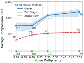
(a) F-EMNIST

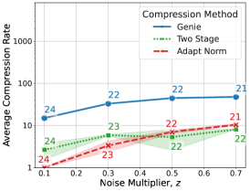
(b) SONWP

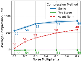
(c) Shakespeare

Figure 2: Our adaptive approaches achieve favorable compression rates without tuning. The ‘Genie’ represents the optimal fixed compression rate obtained via significant hyper parameter tuning. Our adaptive approaches are all $1$-shot using a fixed constant of $0.1$. Text represents the final validation accuracy, with the ‘Genie’ at $\Delta=1\%$.

In this section, we present experimental evaluation of the methods proposed in Section 4 for federated optimization, in standard FL benchmarks. We define the average compression rate of an $T$-round procedure as be relative decrease in the average bits communicated, i.e., $\frac{dT}{\sum_{t=1}^{T}L_{t}+\tilde{L}_{t}}$ where $d$ is the model dimensionality, $L_{t}$ and $\tilde{L}_{t}$ are sizes of first and second sketches at round $t$. This is equivalently the harmonic average of the per-round compression rates.

Setup.

We focus on three common FL benchmarks: Federated EMNIST (F-EMNIST) and Shakespeare represent two relatively easier tasks, and Stack Overflow Next Word Prediction (SONWP) represents a relatively harder task. F-EMNIST is an image classification task, whereas Shakespeare and SONWP are language modelling. We follow the exact same setup (model architectures, hyper parameters) as Chen et al. (2022a) except where noted below. Our full description can be found in Appendix F.

Unlike Chen et al. (2022a), we use fixed clipping (instead of adaptive clipping) and tune the server’s learning rate for each noise multiplier, $z$. As noted by Choquette-Choo et al. (2022), we also zero out high $\ell_{1}$ norm updates $\geq 100$ for improved utility and use their hyper parameters for SONWP.

Defining Feasible Algorithms.

Consider that introducing compression into a DP FL algorithm introduces more noise into its optimization procedure. Thus, we may expect that our algorithms will perform worse than the baseline. We define $\Delta$ to be the max allowed relative drop in utility (validation accuracy) when compared to their baseline without compression. Then, our set of feasible algorithms are those that achieve at least $1-\Delta$ of the baseline performance. This lets us study the privacy-utility tradeoff under a fixed utility and closely matches real-world constraints—often a practitioner will desire an approach that does not significantly impact the model utility, where $\Delta$ captures their tolerance.

Algorithms.

Our baseline is the Genie, which is the method of Chen et al. (2022a), run on the grid of exponentially increasing compression rates $2^{b},b\in[0,13]$. This requires computation that is logarithmic in the interval size and significantly more communication bandwidth in totality—thus, this is unachievable in practice but serves as our best-case upper bound. Our proposed adaptive algorithms are Adapt Norm and Two Stage method, described in Section 4.

Achieving Favorable Compression Without Tuning.

Because the optimal Genie compression rates may be unattainable without significantly increased communication and computation, we instead desire to achieve nontrivial compression rates, as close this genie as possible, but without any (significant) additional computation, while also ensuring that the impact on utility remains negligible. Thus, to ensure minimal impact on utility, we run our adaptive protocols so that the error introduced by compression is much smaller than that which is introduced by DP. We heuristically choose that error from compression can be at most 10% of DP: this choice of this threshold is such that the error is small enough to be dominated by DP and yet large enough for substantial compression rates. We emphasize that we chose this value heuristically and do not tune it.

In extensive experiments across all three datasets (Figure 2), we find that our methods achieve essentially the same utility models (as seen by the colored text). We further find that our methods achieve nontrivial and favorable communication reduction—though still far from the genie, they already recover a significant fraction of the compression rate. This represents a significant gain in computation: to calculate this genie we ran tens of jobs per noise multiplier—for our proposed methods, we run but one.

Comparing our methods, we find that the Adapt Norm approach performs best. It achieves favorable compression rates consistently across all datasets with compression rates that can well adapt to the specific error introduced by DP at a given noise multiplier. For example, we find on the Shakespeare dataset in Figure 2 (c) that the compression-privacy curve follows that of the genie. In contrast, the Two Stage approach typically performs much worse. This is in part due to construction: we require a significant number of warmup rounds (we use $W=75$) to get an estimate of the gradient norm. Because these warmup rounds use no compression, it drastically lowers the (harmonic) average compression rate. We remark that in scenarios where strong priors exist, e.g., when tuning a model on a similar proxy dataset locally prior to deploying in production, it may be possible to significantly reduce or even eliminate $W$ so as to make this approach more competitive. However, our fully-adaptive Adapt Norm approach is able to perform well even without any prior knowledge of the such statistics.

Benchmarking computation overhead.

We remark that sketching is a computationally efficient algorithm requiring computation similar to clipping for encoding and decoding the update. Though our adaptive approaches do introduce minor additional computation (e.g., a second sketch), these do not significantly impact the runtime. In benchmark experiments on F-EMINST, we found that standard DP-Fed Avg takes 3.63s/round, DP-Fed Avg with non-adaptive sketching takes 3.63s/round, and our Adapt Norm approach take 3.69s/round. Noting that our methods may impact convergence, so we also fix the total number of rounds a-priori in all experiments; this provides a fair comparison for all methods where any slow-down in convergence is captured by the utility decrease.

Choosing the relative error from compression ($c_{0}$).

Though we chose $c_{0}=10\%$ heuristically and without tuning, we next run experiments selecting other values of $c_{0}$ to show that our intuition of ensuring the relative error is much smaller leads to many viable values of this hyperparameter. We sweep values representing $\{25,5,1\}\%$ error and compare the utility-compression tradeoff in Appendix A. We find that $c_{0}$ well captures the utility-compression tradeoff, where smaller values consistently lead to higher utility models with less compression, and vice versa. We find that the range of suitable values is quite large, e.g., even as low as $c_{0}=1\%$, non-trivial compression can be attained.

6 Conclusion and Discussion

We design autotuned compression techniques for private federated learning that are compatible with secure aggregation. We accomplish this by creating provably optimal autotuning procedures for federated mean estimation and then mapping them to the federated optimization (learning) setting. We analyze the proposed mean estimation schemes and show that they achieve order optimal error rates with order optimal communication complexity, adapting to the norm of the true mean (Section 3.1) and adapting to the tail-norm of the true mean (Section 3.2). Our results show that we can attain favorable compression rates that recover much of the optimal Genie, in one-shot without any additional computation. Although the $\ell_{2}$ error in mean estimation is a tractable proxy for autotuning compression rate in federated learning, we found that it may not always correlate well with the downstream model accuracy. In particular, in our adaptation of Adapt Tail to federated learning (in Appendix H), we found that that the procedure is able to attain very high compression rates for the federated mean estimation problem, with little overhead in $\ell_{2}$ error, relative to the DP error. However, these compression rates are too high to result in useful model accuracy. So a natural direction for future work is to design procedures which improve upon this proxy in federated learning settings.

Appendix A Additional Figures

F-EMNIST
Relative Error, $c_{0}$	Metric	Noise Multiplier ($z$)
		0.1	0.2	0.3	0.5
N/A, Genie	Validation Accuracy	81.23	79.70	77.68	74.92
	Compression rate, $r$	339	341	1443	2391
0.25	Validation Accuracy	78.87	75.53	77.01	74.97
	Compression rate, $r$	101	212	284	332
0.1	Validation Accuracy	81.34	78.53	77.81	75.36
	Compression rate, $r$	47	94	117	134
0.05	Validation Accuracy	81.84	79.04	78.43	75.66
	Compression rate, $r$	24	47	59	68
0.01	Validation Accuracy	82.51	79.59	78.67	75.56
	Compression rate, $r$	5	9	12	13

Table 1: Adapt Norm is stable with respect to choices in the relative error constant $c_{0}$. We observe that as this constant is increased so that the compression error is larger with respect to the privacy error, the model’s utility degrades and the compression rates obtained increase, and vice versa; this aligns with our expectations as the total error in the FME estimate increases (decreases). However, all choices of constant below $0.1$ lead to viable models with non-trivial compression rates. Results for F-EMNIST with values displaying the mean across 5 runs. Bolded rows represent configurations used in the rest of our experiments.

Shakespeare
Relative Error, $c_{0}$	Metric	Noise Multiplier ($z$)
		0.1	0.2	0.3	0.5	0.7
N/A, Genie	Validation Accuracy	55.41	53.91	52.48	50.44	48.68
	Compression rate, $r$	133	210	342	460	511
0.25	Validation Accuracy	55.71	53.93	52.26	49.12	46.96
	Compression rate, $r$	24	64	117	235	367
0.1	Validation Accuracy	55.77	54.17	52.57	49.87	47.84
	Compression rate, $r$	12	29	49	98	154
0.05	Validation Accuracy	55.89	54.29	52.82	50.23	48.12
	Compression rate, $r$	7	17	27	50	75
0.01	Validation Accuracy	55.83	54.28	52.85	50.66	48.87
	Compression rate, $r$	2	5	8	13	18

Table 2: Adapt Norm is stable with respect to choices in the relative error constant $c_{0}$. We observe that as this constant is increased so that the compression error is larger with respect to the privacy error, the model’s utility degrades and the compression rates obtained increase, and vice versa; this aligns with our expectations as the total error in the FME estimate increases (decreases). However, all choices of constant below $0.1$ lead to viable models with non-trivial compression rates. Results for Shakespere with values displaying the mean across 5 runs. Bolded rows represent configurations used in the rest of our experiments.

SONWP
Relative Error, $c_{0}$	Metric	Noise Multiplier ($z$)
		0.1	0.3	0.5	0.7
N/A, Genie	Validation Accuracy	23.77	22.36	22.07	21.33
	Compression rate, $r$	15	33	45	48
0.25	Validation Accuracy	23.97	22.59	22.06	21.15
	Compression rate, $r$	2	4	12	16
0.1	Validation Accuracy	24.03	22.70	22.12	21.31
	Compression rate, $r$	1	3	7	10
0.05	Validation Accuracy	23.93	22.39	22.14	21.35
	Compression rate, $r$	1	2	4	6
0.01	Validation Accuracy	24.10	22.57	22.17	21.38
	Compression rate, $r$	1	1	2	3

Table 3: Adapt Norm is stable with respect to choices in the relative error constant $c_{0}$. We observe that as this constant is increased so that the compression error is larger with respect to the privacy error, the model’s utility degrades and the compression rates obtained increase, and vice versa; this aligns with our expectations as the total error in the FME estimate increases (decreases). However, all choices of constant below $0.1$ lead to viable models with non-trivial compression rates. Results for SONWP with values displaying the mean across 5 runs. Bolded rows represent configurations used in the rest of our experiments.

Appendix B Missing Details from Section 3

In this section, we provide additional details on FME.

B.1 Instance optimal FME with bounded norm of the mean

Optimal error rate with bounded mean norm.

We consider a problem of DP mean estimation when the data is at the server, but under the assumption that $\left\|{\mu}\right\|\leq M$ with a known $M$. First, we investigate the statistical complexity of the problem, without DP, showing a lower bound on the error of $\Omega(G^{2}\min(M^{2},1/n))$ – see Theorem 8 in Appendix D.1. Secondly, in order to understand the complexity under differential privacy constraint, we study the empirical version of the problem wherein for a fixed dataset, the goal is estimate its empirical mean. Our main result is the following.

Theorem 4.

For any $d,n\in{\mathbb{N}},G,M>0$, define the instance class, $\widehat{\mathcal{P}}_{1}(n,d,G,M)=\left\{{\left\{{z_{i}}\right\}_{i=1}^{n}:z_{i}\in{\mathbb{R}}^{d},\left\|{z_{i}}\right\|\leq G,\left\|{\widehat{\mu}(\left\{{z_{i}}\right\}_{i=1}^{n})}\right\|\leq MG}\right\}$ For any $\epsilon=O(1)$ and $2^{-\Omega(n)}\leq\delta\leq\frac{1}{n^{1+\Omega(1)}}$, we have,

$$\min_{{\mathcal{A}}:{\mathcal{A}}\text{ is }(\epsilon,\delta)-\text{DP}}\max_{D\in\widehat{\mathcal{P}}_{1}(n,d,G,M)}\mathbb{E}\left\|{{\mathcal{A}}(D)-\widehat{\mu}(D)}\right\|^{2}=\Theta\left({G^{2}\,\min\left({M^{2},\frac{d\operatorname{log}\left(1/\delta\right)}{n^{2}\epsilon^{2}}}\right)}\right)$$

We convert the lower bound for the empirical problem to the statistical problem, via a known re-sampling trick (see Bassily et al. [2019], Appendix C). The proof of Theorem 4 is based on reduction to the (standard) DP mean estimation wherein the above assumption on the bound on norm of the mean is absent, for which the optimal error is known [Steinke and Ullman, 2015, Kamath and Ullman, 2020]. Our result above shows that this additional restriction of $\|\widehat{\mu}(\{z_{i}\}_{i=1}^{n})\|\leq MG$ does not make the problem much easier in terms of achievable error. In the interesting regime when $G>M\geq G\sqrt{d\operatorname{log}\left(1/\delta\right)}/(n\epsilon)$, this yields the (same) optimal error with potentially significantly smaller communication.

Instance-specific tightness.

We show that for any dataset with mean $\widehat{\mu}$, the mean-squared error of count-mean sketch (i.e. $R=1$) with added noise of variance $\sigma^{2}$ is exactly $\frac{d-1}{PC}\left\|{\widehat{\mu}}\right\|^{2}+\frac{d\sigma^{2}}{n^{2}}$ – see Lemma 6 for the statement. Therefore, $\left\|{\widehat{\mu}}\right\|$ is the only statistic that controls the MSE of this procedure. Adapting to the norm of mean thus provides a tight instance-specific communication complexity for this method.

B.2 Instance optimal FME with bounded tail-norm of the mean

Lower bound on error:

The error rate in Theorem 3 matches the rate in Eqn. (1), known to be optimal in the worst case, i.e. general values of tail-norms. However, it may be possible to do better in special cases. Towards this, we establish lower bounds for (central) DP mean estimation, where the algorithm designer is given $k<d$ and $\gamma$ and is promised that $\left\|{\mu_{\text{n-tail}({k})}}\right\|\leq\gamma$. For this setting, we present a lower bound on error of $\Omega\left({G^{2}\min\left\{{1,\gamma^{2}+\frac{k}{n^{2}\epsilon^{2}}+\frac{1}{n},\frac{d}{n^{2}\epsilon^{2}}+\frac{1}{n}}\right\}}\right)$. The first and third term are standard, achieved by outputting zero and our procedure (or simply, by Gaussian mechanism) respectively. The second term is new, which is absent from the guarantees of our procedure.

To prove the lower bound, we first show, in Theorem 9, in Section D.1, that the statistical error, without DP, is unchanged, $\Omega\left({\min\left({G^{2},\frac{G^{2}}{n}}\right)}\right)$. Secondly, in order to establish the fundamental limits under differential privacy, we study the empirical version of the problem, where the goal is to estimate the empirical mean, and give the following result.

Theorem 5.

For any $n,d,k\in{\mathbb{N}},G,M,\gamma\geq 0$, define the instance class $\widehat{\mathcal{P}}_{2}(n,d,G,k,\gamma)=\left\{{\left\{{z_{i}}\right\}_{i=1}^{n}:z_{i}\in{\mathbb{R}}^{d},\left\|{z_{i}}\right\|\leq G,\left\|{\widehat{\mu}(D)_{\text{n-tail}({k})}}\right\|^{2}\leq\gamma^{2}}\right\}$. For $\epsilon=O(1)$ and $2^{-\Omega(n)}\leq\delta\leq\frac{1}{n^{1+\Omega(1)}}$, we have

$$\min_{{\mathcal{A}}:{\mathcal{A}}\text{ is }(\epsilon,\delta)\text{-DP}}\max_{D\in{\mathcal{P}}(n,d,G,k,\gamma)}\mathbb{E}\left\|{{\mathcal{A}}(D)-\widehat{\mu}(D)}\right\|^{2}=\Omega\left({G^{2}\min\left\{{1,\gamma^{2}+\frac{k\operatorname{log}\left(1/\delta\right)}{n^{2}\epsilon^{2}},\frac{d\operatorname{log}\left(1/\delta\right)}{n^{2}\epsilon^{2}}}\right\}}\right)$$

We convert the lower bound for the empirical problem to the statistical problem, via a known re-sampling trick (see Bassily et al. [2019], Appendix C). We provide the proof of Theorem 5 in Section D.2.

Achieving the optimal error with small communication:

We show that a simple tweak to our procedure underlying Theorem 3 – adding a Top-$k$ to the unsketched estimate, with exponentially increasing $k$ – suffices to achieve the error in Theorem 5. The procedure is adaptive in $k$, but requires prior knowledge of $\gamma$ and is a biased estimator of the mean. In the following, we abuse notation and write $k_{\text{tail}}(\gamma^{2};\mu)$ which corresponds to plugging $g(k)=\gamma^{2}$ in its definition.

Theorem 6.

For any $\gamma>0$, Algorithm 2 with the same parameter settings as in Theorem 3 except with $k_{j}=2^{j}$ and $\overline{\gamma}_{j}=16\left({\gamma G+\frac{G\sqrt{\operatorname{log}\left(8\operatorname{log}\left(d\right)/\beta\right)}}{\sqrt{m}}+\sqrt{k_{j}}\frac{\sigma}{n}}\right)+\tilde{\alpha}$ satisfies $(\epsilon,\delta)$-DP. With probability at least $1-\beta$, the final output satisfies,

$$\left\|{\bar{\mu}-\mu}\right\|^{2}=\tilde{O}\left({G^{2}\left({\gamma^{2}+\frac{1}{n}+\frac{k_{\text{tail}}(\gamma^{2};\mu)\operatorname{log}\left(1/\delta\right)}{n^{2}\epsilon^{2}}}\right)}\right),$$

the total per-client communication complexity is $\tilde{O}\left({k_{\text{tail}}(\gamma^{2};\mu)}\right)$ and number of rounds is $\lfloor\operatorname{log}\left(d\right)\rfloor$.

We provide the proof of Theorem 6 in Appendix C.

Optimal communication complexity:

Next, we investigate the communication complexity of multi-round SecAgg-compatible, potentially biased, schemes with prior knowledge of $k$ and $\gamma$ such that $\left\|{\mu_{\text{n-tail}({k})}}\right\|\leq\gamma$. Our main result is the following.

Theorem 7.

Let $d,n,k,K\in{\mathbb{N}},d\geq 2k,\epsilon,\delta,G,\alpha,\gamma>0$. Define ${\mathcal{P}}_{2}(d,G,\gamma,k)=\left\{{{\mathcal{D}}\text{ over }{\mathbb{R}}^{d}:\left\|{z}\right\|\leq G,z\sim{\mathcal{D}},\text{ and }\left\|{\mu({\mathcal{D}})_{\text{n-tail}({k})}}\right\|^{2}\leq\gamma^{2}}\right\}$. For any $K$, any protocol ${\mathcal{A}}$ in the class of $K$-round, SecAgg-compatible protocols (see Appendix E for details) such that its MSE, $\mathbb{E}_{D\sim{\mathcal{D}}^{n}}[\left\|{{\mathcal{A}}(D)-\mu}\right\|^{2}]\leq\alpha^{2}$ for all ${\mathcal{D}}\in{\mathcal{P}}_{2}(d,G,\gamma,k)$, there exists a distribution ${\mathcal{D}}\in{\mathcal{P}}_{2}(d,G,\gamma,k)$, such that on dataset $D\sim{\mathcal{D}}^{n}$, w.p. 1, the total per-client communication complexity is $\Omega(k\operatorname{log}\left(Gd/k\alpha\right))$.

Plugging in the error $\alpha^{2}$ from Theorem 6 establishes that complexity complexity of Theorem 6 is tight upto poly-logarithmic factors.

Instance-specific tightness.

We show, in Lemma 5 in Appendix C, that for any $P$, $C=\Omega(Pk)$ and $R=\operatorname{log}\left(d\right)$, for any dataset with mean $\widehat{\mu}$, the error of the count median-of-means sketch underlying Theorem 6 with added noise of variance $\sigma^{2}$, with high probability, is $\Omega\left({G^{2}\left\|{\widehat{\mu}_{\text{n-tail}({k})}}\right\|^{2}+\sigma^{2}k}\right)$.

Discussion on Theorem 3 vs Theorem 6:

While the error in procedure defined in Theorem 3 may be larger than that in Theorem 6, the former has some attractive properties that make it useful in practice. Specifically, it is unbiased which is desirable in stochastic optimization and it does not require knowledge of any new hyper-parameter $\gamma$, which is unclear how to adapt to. Further, the additional top $k$ operation, which is the sole difference between the two procedures, does not seem to provide significant benefits in our downstream FL experiments. Consequently, we use the procedure underlying Theorem 3 in our experimental settings, and defer detailed investigation of the method in Theorem 6 to future work.

Appendix C Proofs of Error Upper Bounds for FME

C.1 Useful Lemmas

In this section, we collect and state lemmas that will be used in the proofs of the main results.

Lemma 1.

Kane and Nelson [2014] For any $i\in[R]$, CountSketch matrix $S^{(i)}\in{\mathbb{R}}^{PC\times d}$ with $P=\Omega\left({\tau^{-1}\operatorname{log}\left(1/\beta\right)}\right)$ and $C=\frac{1}{\tau}$ satisfies that, for any $z\in{\mathbb{R}}^{d}$, with probability at least $1-\beta$, $\left({1-\tau}\right)\left\|{z}\right\|^{2}\leq\left\|{S^{(i)}z}\right\|^{2}\leq\left({1+\tau}\right)\left\|{z}\right\|^{2}$

The result below shows that Count-median-of-means sketch preserves norms and heavy hitters.

Lemma 2.

Let $0<\alpha,\tau,\beta<1$ and $k,d\in{\mathbb{N}}$ and $k\leq d$. For $P=\Theta\left({\tau^{-1}\operatorname{log}\left(2R/\beta\right)}\right),C=\max\left({8Pk,\frac{k}{8P\alpha},\frac{1}{\tau}}\right)$ and $R=\lceil 2\operatorname{log}\left(2d/\beta\right)\rceil$, the sketch $S$ satisfies that for any $z\in{\mathbb{R}}^{d}$, with probability at least $1-\beta$,

1. JL property:

   $$\left({1-\tau}\right)\left\|{z}\right\|^{2}\leq\left\|{S^{(i)}z}\right\|^{2}\leq\left({1+\tau}\right)\left\|{z}\right\|^{2}\ \forall i\in[R]$$

2. $\ell_{\infty}$ guarantee: Let $\bar{z}=U(S(z))$, then,

   $$\left({\bar{z}_{q}-z_{q}}\right)^{2}\leq\frac{\alpha\left\|{z_{\text{tail}(k)}}\right\|^{2}}{k}\ \forall q\in[d]$$

3. Sparse recovery:

   1. Let $\tilde{z}=\text{Top}_{k}(\bar{z})$

      $$\left\|{\tilde{z}-z}\right\|_{2}^{2}\leq\left({1+7\sqrt{\alpha})}\right)\left\|{z_{\text{tail}(k)}}\right\|^{2}$$

   2. Let $\widehat{z}=\text{Top}_{2k}(\bar{z})$

      $$\left\|{\widehat{z}-z}\right\|_{2}^{2}\leq\left({1+10\alpha}\right)\left\|{z_{\text{tail}(k)}}\right\|^{2}$$

   where $\left\|{z_{\text{tail}(k)}}\right\|=\min_{\tilde{z}:\left\|{\tilde{z}}\right\|_{0}\leq k}\left\|{z-\tilde{z}}\right\|_{2}$.

Proof.

$P=1$ corresponds to the standard Countsketch based method. For $P>1$, we modify the analysis as follows. The first part directly follows from the result of Kane and Nelson [2014], stated as Lemma 1, which gave a construction of a sparse Johnson-Lindenstrauss transform based on CountSketch.

We now proceed to the second part. Let $H_{k}\subseteq[d]$ denote the indices of $k$ largest co-ordinates of $z$. We first consider the estimate of $z_{q}$ based on one row ($i$-th row), which is give as,

$$\bar{z}^{(i)}_{q} =\left({{S^{(i)}}^{\top}S^{(i)}z}\right)_{q}=\frac{1}{P}\sum_{j=1}^{d}\sum_{p=1}^{P}s^{(i)}_{p}(j)s^{(i)}_{p}(q)\mathbbm{1}\left({h^{(i)}_{p}(j)=h_{p}^{(i)}(q)}\right)z_{j}$$

$$=z_{q}+\underbrace{\frac{1}{P}\sum_{j=1,j\neq q}^{d}\sum_{p=1}^{P}s^{(i)}_{p}(j)s^{(i)}_{p}(q)\mathbbm{1}\left({h^{(i)}_{p}(j)=h_{p}^{(i)}(q)}\right)z_{j}}_{=:E}$$

From moment assumptions, $\mathbb{E}[E]=0$ which gives us that $\mathbb{E}[\bar{z}^{(i)}_{q}]=z_{q}$. We now decompose the error into two terms,

$$E_{H_{k}} =\frac{1}{P}\sum_{j\in{H_{k}},j\neq q}\sum_{p=1}^{P}s^{(i)}_{p}(j)s^{(i)}_{p}(q)\mathbbm{1}\left({h^{(i)}_{p}(j)=h_{p}^{(i)}(q)}\right)z_{j}$$

$$E_{T_{k}} =\frac{1}{P}\sum_{j\not\in{H_{k}},j\neq q}\sum_{p=1}^{P}s^{(i)}_{p}(j)s^{(i)}_{p}(q)\mathbbm{1}\left({h^{(i)}_{p}(j)=h_{p}^{(i)}(q)}\right)z_{j}$$

By construction,

$$\mathbb{P}\left({E_{H_{k}}\neq 0}\right)\leq\mathbb{P}\left({\exists j\in{H_{k}},p\in[P]:h^{(i)}_{p}(j)=h^{(i)}_{p}(q)}\right)\leq\frac{Pk}{C}\leq\frac{1}{8}$$

for $C\geq 8Pk$. For the other term, we directly compute its second moment,

$$\mathbb{E}[E_{T_{k}}^{2}] =\mathbb{E}\left[\left({\frac{1}{P}\sum_{j\not\in{H_{k}},j\neq q}\sum_{p=1}^{P}s^{(i)}_{p}(j)s^{(i)}_{p}(q)\mathbbm{1}\left({h^{(i)}_{p}(j)=h_{p}^{(i)}(q)}\right)z_{j}}\right)^{2}\right]$$

$$=\frac{1}{P^{2}}\sum_{j\not\in{H_{k}},j\neq q}\sum_{p=1}^{P}\mathbb{E}\left[\mathbbm{1}\left({h^{(i)}_{p}(j)=h_{p}^{(i)}(q)}\right)\right]z_{j}^{2}+0$$

$$\leq\frac{1}{PC}\left\|{z_{\text{tail}(k)}}\right\|^{2}$$

Therefore for $C\geq\frac{k}{8P\alpha}$, from Chebyshev’s inequality, $E_{T_{k}}\leq\frac{\sqrt{\alpha}\left\|{z_{\text{tail}(k)}}\right\|}{\sqrt{k}}$ with probability at least $7/8$. Combining, for $C=\max\left({\frac{k}{8P\alpha},8Pk}\right)$, with probability at least $3/4$,

$$\left({\bar{z}_{q}^{(i)}-z_{q}}\right)^{2}\leq\frac{\alpha\left\|{z_{\text{tail}(k)}}\right\|^{2}}{k}$$

With $R=\lfloor 2\operatorname{log}\left(1/\beta^{\prime}\right)\rfloor$, and $\bar{z}_{q}=\text{median}\left\{{\bar{z}_{q}^{(i)}}\right\}_{i=1}^{R}$; using the standard boosting guarantee based on a median of estimates, we have, with probability at least $1-\beta^{\prime}$,

$$\left({\bar{z}_{q}-z_{q}}\right)^{2}\leq\frac{\alpha\left\|{z_{\text{tail}(k)}}\right\|^{2}}{k}.$$

Setting $\beta^{\prime}=\frac{\beta}{2d}$ and doing a union bound on all coordinates gives that with probability at least $1-\beta$, for all $q\in[d]$,

$$\left({\bar{z}_{q}-z_{q}}\right)^{2}\leq\frac{\alpha\left\|{z_{\text{tail}(k)}}\right\|^{2}}{k}.$$

The third item in the Lemma statement is based on converting the $\ell_{\infty}$ to $\ell_{2}$ guarantee; specifically, instantiating Lemma 3 with $\Delta^{2}=\frac{\alpha\left\|{z_{\text{tail}(k)}}\right\|^{2}}{k}$ gives us,

$$\left\|{\tilde{z}-z}\right\|^{2} \leq\left({1+5\alpha+2\sqrt{\alpha}}\right)\left\|{z_{\text{tail}(k)}}\right\|^{2}$$

$$\leq\left({1+7\sqrt{\alpha}}\right)\left\|{z_{\text{tail}(k)}}\right\|^{2}.$$

Similarly, from Lemma 3, we get,

$$\left\|{\widehat{z}-z}\right\|^{2}\leq\left({1+10\alpha}\right)\left\|{z_{\text{tail}(k)}}\right\|^{2},$$

which completes the proof. ∎

Lemma 3.

Let $z\in{\mathbb{R}}^{d}$ and $\bar{z}\in{\mathbb{R}}^{d}$ such that $\left\|{\bar{z}-z}\right\|_{\infty}^{2}\leq\Delta^{2}$. Define $\tilde{z}=\text{Top}_{k}(\bar{z})$ and $\widehat{z}=\text{Top}_{2k}(\bar{z})$. Then,

$$\left\|{z-\bar{z}}\right\|_{2}^{2}\leq 5k\Delta^{2}+\left\|{z_{\text{tail}(k)}}\right\|^{2}+2\Delta\sqrt{k}\left\|{z_{\text{tail}(k)}}\right\|$$

$$\left\|{z-\widehat{z}}\right\|_{2}^{2}\leq 10k\Delta^{2}+\left\|{z_{\text{tail}(k)}}\right\|^{2}$$

Proof.

This is a fairly standard fact, though typically not presented in the form above (see, for instance Price and Woodruff [2011]). We give a proof for completeness and its use in many parts of the manuscript. Let $I$ denote the indices of top $k$ co-ordinates of $z$ and let $\tilde{I}$ and $\widehat{I}$ denote the top $k$ and top $2k$ co-ordinates of $\bar{z}$. We proceed with the first part of the lemma. Note that,

$$\left\|{z-\tilde{z}}\right\|^{2}=\left\|{z-\bar{z}_{\tilde{I}}}\right\|^{2}=\left\|{(z-\bar{z})_{\tilde{I}}}\right\|^{2}+\left\|{z_{\tilde{I}^{c}}}\right\|^{2}$$ (4)

where $\tilde{I}^{c}$ denotes the complement set of $\tilde{I}$. The first term is bounded as $\left\|{(z-\bar{z})_{\tilde{I}}}\right\|^{2}\leq\left|{\tilde{I}}\right|\left\|{z-\bar{z}}\right\|_{\infty}^{2}=k\Delta^{2}$. We decompose the second term $\left\|{z_{\tilde{I}^{c}}}\right\|^{2}$ as follows,

$$\left\|{z_{\tilde{I}^{c}}}\right\|^{2}=\left\|{z_{I\backslash\tilde{I}}}\right\|^{2}+\left\|{z_{I^{c}}}\right\|^{2}-\left\|{z_{\tilde{I}\backslash I}}\right\|^{2}$$

Let $a=\max_{i\in I\backslash\tilde{I}}z_{i}$ and $b=\min_{i\in\tilde{I}\backslash I}z_{i}$. From the $\ell_{\infty}$ guarantee and the fact that the sets $I$ and $\tilde{I}$ are indices of top $k$ elements of $z$ and $\tilde{z}$ respectively, we have that $(a-b)^{2}\leq 4\left\|{\bar{z}-z}\right\|_{\infty}^{2}\leq 4\Delta^{2}$. We note consider two cases (a). $b\leq 0$ and $b>0$. In the first case, we have that $a\leq 2\Delta$. Plugging all these simplifications in Eqn. (4), we get,

$$\left\|{z-\tilde{z}}\right\|^{2} \leq k\Delta^{2}+\left\|{z_{I^{c}}}\right\|^{2}+\left\|{z_{I\backslash\tilde{I}}}\right\|^{2}-\left\|{z_{\tilde{I}\backslash I}}\right\|^{2}$$

$$\leq k\Delta^{2}+\left\|{z_{I^{c}}}\right\|^{2}+\left|{I\backslash\tilde{I}}\right|a^{2}$$

$$\leq k\Delta^{2}+\left\|{z_{I^{c}}}\right\|^{2}+4k\Delta^{2}=\left\|{z_{I^{c}}}\right\|^{2}+5k\Delta^{2}$$

In the other case (b). $b>0$, we get,

$$\left\|{z-\tilde{z}}\right\|^{2} \leq k\Delta^{2}+\left\|{z_{I^{c}}}\right\|^{2}+\left\|{z_{I\backslash\tilde{I}}}\right\|^{2}-\left\|{z_{\tilde{I}\backslash I}}\right\|^{2}$$

$$\leq k\Delta^{2}+\left\|{z_{I^{c}}}\right\|^{2}+\left|{I\backslash\tilde{I}}\right|a^{2}-\left|{\tilde{I}\backslash\tilde{I}}\right|b^{2}$$

$$=k\Delta^{2}+\left\|{z_{I^{c}}}\right\|^{2}+\left|{I\backslash\tilde{I}}\right|\left({a^{2}-b^{2}}\right)$$

$$\leq k\Delta^{2}+\left\|{z_{I^{c}}}\right\|^{2}+\left|{I\backslash\tilde{I}}\right|\left({(b+2\Delta)^{2}-b^{2}}\right)$$

$$\leq k\Delta^{2}+\left\|{z_{I^{c}}}\right\|^{2}+2\Delta\left|{I\backslash\tilde{I}}\right|b+4\left|{I\backslash\tilde{I}}\right|\Delta^{2}$$

$$\leq k\Delta^{2}+\left\|{z_{I^{c}}}\right\|^{2}+2\Delta\sqrt{\left|{I\backslash\tilde{I}}\right|}\left\|{z_{I^{c}}}\right\|+4k\Delta^{2}$$

$$\leq 5k\Delta^{2}+\left\|{z_{I^{c}}}\right\|^{2}+2\Delta\sqrt{k}\left\|{z_{I^{c}}}\right\|$$

where the first equality follows since $\left|{I}\right|=\left|{\tilde{I}}\right|=k$, and the second last inequality follows since $\sqrt{\left|{I\backslash\tilde{I}}\right|}b\left\|{z_{I^{c}}}\right\|$ and $b$ is value of the the minimal element in $I\backslash\tilde{I}$.

Finally, note that $\left\|{z_{I^{c}}}\right\|=\left\|{z_{\text{tail}(k)}}\right\|$. Hence, combining the two cases yields the statement claimed in the lemma.

The second part follows analogously. In particular, repeating the initial steps gives us

$$\left\|{z-\widehat{z}}\right\|^{2} \leq 2k\Delta^{2}+\left\|{z_{I^{c}}}\right\|^{2}+\left\|{z_{I\backslash\widehat{I}}}\right\|^{2}-\left\|{z_{\widehat{I}\backslash I}}\right\|^{2}.$$

Defining $a$ and $b$ as before and considering the two cases give us that in the first case (a). $b\leq 0$, we have,

$$\left\|{z-\widehat{z}}\right\|^{2} \leq 2k\Delta^{2}+\left\|{z_{I^{c}}}\right\|^{2}+\left\|{z_{I\backslash\widehat{I}}}\right\|^{2}$$

$$\leq 2k\Delta^{2}+\left\|{z_{I^{c}}}\right\|^{2}+\left|{I\backslash\widehat{I}}\right|a^{2}$$

$$\leq 2k\Delta^{2}+\left\|{z_{I^{c}}}\right\|^{2}+4k\Delta^{2}$$

$$=6k\Delta^{2}+\left\|{z_{I^{c}}}\right\|^{2}.$$

In the second case, let $\widehat{k}=\left|{I\backslash\widehat{I}}\right|$; note that $\left|{\widehat{I}\backslash I}\right|=k+\widehat{k}$. Therefore,

$$\left\|{z-\widehat{z}}\right\|^{2} \leq 2k\Delta^{2}+\left\|{z_{I^{c}}}\right\|^{2}+\left\|{z_{I\backslash\widehat{I}}}\right\|^{2}-\left\|{z_{\widehat{I}\backslash I}}\right\|^{2}$$

$$\leq 2k\Delta^{2}+\left\|{z_{I^{c}}}\right\|^{2}+\widehat{k}a^{2}-(k+\widehat{k})b^{2}$$

$$\leq 2k\Delta^{2}+\left\|{z_{I^{c}}}\right\|^{2}+4\widehat{k}\Delta^{2}+4\widehat{k}b\Delta-kb^{2}$$

$$=-k\left({b-2\frac{\widehat{k}\Delta}{k}}\right)^{2}+\frac{4\widehat{k}^{2}\Delta^{2}}{k}+2k\Delta^{2}+4\widehat{k}\Delta^{2}+\left\|{z_{I^{c}}}\right\|^{2}$$

$$\leq 10k\Delta^{2}+\left\|{z_{I^{c}}}\right\|^{2}.$$

where in the last inequality, we used that $\widehat{k}\leq k$. Combining the two cases finishes the proof. ∎

The following result gives a heavy hitter guarantee for count-median-of-means sketch with noise.

Lemma 4.

Let $z\in{\mathbb{R}}^{d}$, $R,C,P$ be parameters of Count-median-of-means sketch $S$ and let $\xi\sim{\mathcal{N}}(0,\sigma^{2}{\mathbb{I}})$. Let $\bar{z}=U\left({S(z)+\xi}\right)$. For $C\geq\max\left({8Pk,\frac{k}{8P\alpha}}\right)$ and $R=\lceil 2\operatorname{log}\left(2d/\beta\right)\rceil$ gives us that with probability at least $1-\beta$,

$$\left\|{\bar{z}-z}\right\|_{\infty}^{2}\leq\frac{2\alpha\left\|{z_{\text{tail}(k)}}\right\|^{2}}{k}+\sigma^{2}$$

Let $\tilde{z}=\text{Top}_{k}(\bar{z})$ and $\widehat{z}=\text{Top}_{2k}(\bar{z})$. With probability at least $1-\beta$, we have

$$\left\|{\tilde{z}-z}\right\|_{2}^{2}\leq 2\left({1+7\sqrt{\alpha}}\right)\left\|{z_{\text{tail}(k)}}\right\|^{2}+5k\sigma^{2}$$

$$\left\|{\widehat{z}-z}\right\|_{2}^{2}\leq\left({1+20\alpha}\right)\left\|{z_{\text{tail}(k)}}\right\|^{2}+10k\sigma^{2}$$

Proof.

The proof extends the analysis in Pagh and Thorup [2022] which was limited to count-sketch $(P=1)$. Specifically, we apply Lemma 3.4 in Pagh and Thorup [2022] plugging in an estimate of one row error obtained from our sketch. In the proof of Lemma 2, for $C\geq\max\left({8Pk,\frac{k}{8P\alpha}}\right)$, for one row estimate $\bar{z}^{(i)}$, we have that with probability $\geq 3/4$,

$$\left\|{\bar{z}^{(i)}-z}\right\|^{2}_{\infty}\leq\frac{\alpha\left\|{z_{\text{tail}(k)}}\right\|^{2}}{k}$$

For a fixed coordinate $q$, let $\bar{z}_{q}^{(i)}$ denote its estimate from the $i$-th row of the count sketch. We have,

$$\bar{z}_{q}^{(i)} =\underbrace{z_{q}+\frac{1}{P}\sum_{j=1,j\neq q}^{d}\sum_{p=1}^{P}s^{(i)}_{p}(j)s^{(i)}_{p}(q)\mathbbm{1}\left({h^{(i)}_{p}(j)=h_{p}^{(i)}(q)}\right)z_{j}}_{=:A}+\underbrace{\frac{1}{\sqrt{P}}\sum_{p=1}^{P}s^{(i)}_{p}(q)\xi_{p}^{i}}_{=:B}$$

The reason that the second term has $\sqrt{P}$ in the denominator and not $P$ is because the noise is added after sketching, which itself performs division by $\sqrt{P}$ operation. Now, $A$ is the original non-private estimate and $B$ is the additional noise. Since $\xi_{p}^{j}\sim{\mathcal{N}}(0,\sigma^{2})$ and $s_{p}^{(i)}$ are random signs, the random variable $B\sim{\mathcal{N}}(0,\sigma^{2})$. Applying Lemma 3.4 from Pagh and Thorup [2022] gives us that for $\Delta^{2}>\frac{\alpha\left\|{z_{\text{tail}(k)}}\right\|^{2}}{k}$, the mean estimate $\bar{z}$, with probability $1-2d\operatorname{exp}\left(-\frac{R\min\left({1,\frac{\Delta^{2}}{\sigma^{2}}}\right)}{2}\right)$, satisfies

$$\left\|{\bar{z}^{(i)}-z}\right\|^{2}_{\infty}\leq\Delta^{2}$$

We set $\Delta^{2}=\max\left({\frac{2\alpha\left\|{z_{\text{tail}(k)}}\right\|^{2}}{k},\sigma^{2}}\right)$ – note that with this setting, the success probability is at least $1-2d\operatorname{exp}\left(-\frac{R}{2}\right)$. Hence, setting $R=\lceil 2\operatorname{log}\left(2d/\beta\right)\rceil$ yields the claimed $\ell_{\infty}$ guarantee with probability $1-\beta$. For the Top $k$ and Top $2k$ guarantees, we apply Lemma 3 with the above $\Delta$, which yields,

$$\left\|{\tilde{z}-z}\right\|^{2} \leq 5k\left({\frac{2\alpha\left\|{z_{\text{tail}(k)}}\right\|^{2}}{k}+\sigma^{2}}\right)+\left\|{z_{\text{tail}(k)}}\right\|^{2}+2\sqrt{k}\left\|{z_{\text{tail}(k)}}\right\|\left({\frac{2\sqrt{\alpha\left\|{z_{tail}(k)}\right\|}}{\sqrt{k}}+\sigma}\right)$$

$$=\left({1+14\sqrt{\alpha}}\right)\left\|{z_{\text{tail}(k)}}\right\|^{2}+5k\sigma^{2}+2\sqrt{k}\left\|{z_{\text{tail}(k)}}\right\|\sigma$$

$$\leq 2\left({1+7\sqrt{\alpha}}\right)\left\|{z_{\text{tail}(k)}}\right\|^{2}+5k\sigma^{2},$$

where the last inequality follows from AM-GM inequality. Similarly, from Lemma 3, we get

$$\left\|{\widehat{z}-z}\right\|^{2}\leq\left({1+20\alpha}\right)\left\|{z_{\text{tail}(k)}}\right\|^{2}+10k\sigma^{2},$$

which finishes the proof. ∎

In the following, we give a lower bound on the error of count median-of-means sketch with noise, for any instance.

Lemma 5.

Let $R,C,P$ be parameters of Count-median-of-means sketch $S$ and let $\xi_{i}=[\xi^{1}_{i},\xi^{2}_{i},\cdots,\xi^{R}_{i}]^{\top}$, where $\xi_{i}^{j}\sim{\mathcal{N}}(0,\sigma^{2}{\mathbb{I}}_{PC})$ for all $i\in[n],j\in[R]$. Consider any dataset $D=\left\{{z_{1},z_{2},\cdots,z_{n}}\right\}$ and let $\tilde{\mu}=\text{Top}_{k}\left({U\left({\frac{1}{n}\sum_{i=1}^{n}S(z_{i})+\xi_{i}}\right)}\right)$. For $C\geq 100Pk$, and $R=\lceil 800\operatorname{log}\left(2d/\beta\right)\rceil$ with probability at least $1-\beta$,

$$\left\|{\tilde{\mu}-\widehat{\mu}}\right\|^{2}\geq\frac{\left\|{\widehat{\mu}_{\text{tail}(k)}}\right\|^{2}}{2}+0.125\sigma^{2}k$$

Proof.

Since the sketching operation is linear, it suffices to show the result for sketching the mean of the dataset, $\widehat{\mu}:=\frac{1}{n}\sum_{i=1}^{n}z_{i}$. For a fixed coordinate $q$, let $\bar{\mu}_{q}^{(i)}$ denote its estimate from the $i$-th row of the count-median-of-means sketch. We have,

$$\left({\bar{\mu}_{q}^{(i)}-\widehat{\mu}_{q}}\right)^{2} =\left({\underbrace{\frac{1}{P}\sum_{j=1,j\neq q}^{d}\sum_{p=1}^{P}s^{(i)}_{p}(j)s^{(i)}_{p}(q)\mathbbm{1}\left({h^{(i)}_{p}(j)=h_{p}^{(i)}(q)}\right)\widehat{\mu}_{j}}_{=:A}+\underbrace{\frac{1}{\sqrt{P}}\sum_{p=1}^{P}s^{(i)}_{p}(q)\xi_{p}^{i}}_{=:B}}\right)^{2}$$

$$=A^{2}+B^{2}+2AB\geq B^{2}-2\left|{A}\right|\left|{B}\right|$$

Since $\xi_{p}^{j}\sim{\mathcal{N}}(0,\sigma^{2})$ and $s_{p}^{(i)}$ are random signs, the random variable $B\sim{\mathcal{N}}(0,\sigma^{2})$. Using the CDF table for the normal distribution, we have that with

$$\mathbb{P}\left({B^{2}\geq 4\sigma^{2}}\right)=2\mathbb{P}_{X\sim{\mathcal{N}}(0,1)}\left({X\geq 1}\right)\leq 0.04$$

Similarly,

$$\mathbb{P}\left({B^{2}\leq 0.25\sigma^{2}}\right)=1-\mathbb{P}\left({B^{2}>0.25\sigma^{2}}\right)=1-2\mathbb{P}_{X\sim{\mathcal{N}}(0,1)}\left({X>0.5}\right)\leq 0.4$$

With $C\geq\max\left({100Pk,\frac{k}{8P\alpha}}\right)$ as in the proof of Lemma 2, $\left|{A}\right|\leq\frac{\sqrt{\alpha}\left\|{\widehat{\mu}}\right\|_{\text{tail}(k)}}{\sqrt{k}}$ with probability at least $0.99$. Hence, with probability at least $0.55$, we have that

$$\left({\bar{\mu}_{q}^{(i)}-\widehat{\mu}_{q}}\right)^{2}\geq 0.25\sigma^{2}-\frac{4\sigma\sqrt{\alpha}\left\|{\widehat{\mu}_{\text{tail}(k)}}\right\|}{\sqrt{k}}=:\varepsilon^{2}$$

We now argue amplification for the median: Define $I_{q}^{i}=\mathbbm{1}\left({\widehat{\mu}_{q}\leq\bar{\mu}_{q}^{i}\leq\widehat{\mu}_{q}+\varepsilon}\right)$. Note that $\mathbb{E}I_{q}^{i}\leq 0.45$. Then,

$$\mathbb{P}\left({\widehat{\mu}_{q}\leq\bar{\mu}_{q}\leq\widehat{\mu}_{q}+\varepsilon}\right)\leq\mathbb{P}\left({\sum_{i=1}^{R}I_{q}^{i}\geq\frac{R}{2}}\right)\leq\mathbb{P}\left({\sum_{i=1}^{R}\left({I_{q}^{i}-\mathbb{E}I_{q}^{i}}\right)\geq 0.05R}\right)\leq\operatorname{exp}\left(-\frac{R}{800}\right)=\frac{\beta}{2d}$$

by setting of $R$. Now, similarly, we have

$$\mathbb{P}\left({\widehat{\mu}_{q}\geq\bar{\mu}_{q}\geq\widehat{\mu}_{q}-\varepsilon}\right)\leq\frac{\beta}{2d}$$

Combining both gives us that with probability at least $1-\beta$, for all $q\in[d]$

$$\left({\bar{\mu}_{q}-\widehat{\mu}_{q}}\right)^{2}\geq\varepsilon^{2}$$ (5)

Now, let $\tilde{\mu}=\text{Top}_{k}\left({U\left({\frac{1}{n}\sum_{i=1}^{n}S(z_{i})+\xi_{i}}\right)}\right)$ and let $\tilde{I}$ be the set of coordinates achieving its Top $k$. We have,

$$\left\|{\tilde{\mu}-\widehat{\mu}}\right\|^{2}=\left\|{\tilde{\mu}_{\tilde{I}}-\widehat{\mu}_{\tilde{I}}+\widehat{\mu}_{\tilde{I}^{c}}}\right\|^{2}=\left\|{\left({\tilde{\mu}-\widehat{\mu}}\right)_{\tilde{I}}}\right\|^{2}+\left\|{\widehat{\mu}_{{\tilde{I}}^{c}}}\right\|^{2}\geq\left\|{\left({\tilde{\mu}-\widehat{\mu}}\right)_{\tilde{I}}}\right\|^{2}+\left\|{\widehat{\mu}_{\text{tail}(k)}}\right\|^{2}$$

For the other term, from Eqn. (5), we have

$$\left\|{\left({\tilde{\mu}-\widehat{\mu}}\right)_{\tilde{I}}}\right\|^{2}\geq k\varepsilon^{2}$$

Combining, we get,

$$\left\|{\tilde{\mu}-\widehat{\mu}}\right\|^{2}\geq\left\|{\widehat{\mu}_{\text{tail}(k)}}\right\|^{2}+k\varepsilon^{2}=\left\|{\widehat{\mu}_{\text{tail}(k)}}\right\|^{2}+0.25\sigma^{2}k-4\sigma\sqrt{k}\sqrt{\alpha}\left\|{\widehat{\mu}_{\text{tail}(k)}}\right\|$$

Consider two cases:

Case 1

: $\left\|{\widehat{\mu}_{\text{tail}(k)}}\right\|\geq 8\sigma\sqrt{k}\sqrt{\alpha}$. Note that

$$\left\|{\widehat{\mu}_{\text{tail}(k)}}\right\|^{2}-4\sigma\sqrt{k}\sqrt{\alpha}\left\|{\widehat{\mu}_{\text{tail}(k)}}\right\|\geq\frac{\left\|{\widehat{\mu}_{\text{tail}(k)}}\right\|^{2}}{2}\iff\left\|{\widehat{\mu}_{\text{tail}(k)}}\right\|\geq 8\sigma\sqrt{k}\sqrt{\alpha}$$

In this case, the bound becomes,

$$\left\|{\tilde{\mu}-\widehat{\mu}}\right\|^{2}\geq\frac{\left\|{\widehat{\mu}_{\text{tail}(k)}}\right\|^{2}}{2}+0.25\sigma^{2}k$$

Case 2

: $\left\|{\widehat{\mu}_{\text{tail}(k)}}\right\|\leq\frac{0.125\sigma\sqrt{k}}{4\sqrt{\alpha}}$. Note that

$$0.25\sigma^{2}k-4\sigma\sqrt{k}\sqrt{\alpha}\left\|{\widehat{\mu}_{\text{tail}(k)}}\right\|\geq 0.125\sigma^{2}k\iff\left\|{\widehat{\mu}_{\text{tail}(k)}}\right\|\leq\frac{0.125\sigma\sqrt{k}}{4\sqrt{\alpha}}$$

In this case, the bound becomes,

$$\left\|{\tilde{\mu}-\widehat{\mu}}\right\|^{2}\geq\left\|{\widehat{\mu}_{\text{tail}(k)}}\right\|^{2}+0.125\sigma^{2}k$$

We now set $\alpha$ to make sure the two cases exhaust all the possibilities. In particular,

$$8\sigma\sqrt{k}\sqrt{\alpha}=\frac{0.125\sigma\sqrt{k}}{4\sqrt{\alpha}}\iff\alpha=\frac{1}{128}$$

Combining, this gives us,

$$\left\|{\tilde{\mu}-\widehat{\mu}}\right\|^{2}\geq\frac{\left\|{\widehat{\mu}_{\text{tail}(k)}}\right\|^{2}}{2}+0.125\sigma^{2}k$$

which completes the proof. ∎

In the following, we compute the mean-squared error of count-mean sketch with noise, for any instance.

Lemma 6.

For the count-median-of-means sketching operation described in Section 3.2, with $R=1$ and $\xi_{i}\sim{\mathcal{N}}(0,\sigma^{2}{\mathbb{I}}_{PC}),i\in[n]$, we have that for any dataset $D=\left\{{z_{i}}\right\}_{i=1}^{n}$ with $z_{i}\in{\mathbb{R}}^{d}$

$$\mathbb{E}\left\|{U\left({\frac{1}{n}\sum_{i=1}^{n}S(z_{i})+\xi_{i}}\right)-z}\right\|^{2}=\frac{d-1}{PC}\left\|{\widehat{\mu}(D)}\right\|^{2}+d\sigma^{2}$$

Proof.

Since the sketching operation is linear, it suffices to show the result for sketching the mean of the dataset, $\widehat{\mu}:=\frac{1}{n}\sum_{i=1}^{n}z_{i}$. Further, since $R=1$, the sketching and unsketching operation simplifies and we get,

$$\mathbb{E}\left\|{\left({S^{(1)}}\right)^{\top}\left({S^{(1)}\widehat{\mu}+\xi}\right)-\widehat{\mu}}\right\|^{2} =\mathbb{E}\left\|{\left({S^{(1)}}\right)^{\top}S^{(1)}\widehat{\mu}-\widehat{\mu}}\right\|^{2}+\mathbb{E}\left\|{\left({S^{(1)}}\right)^{\top}S^{(1)}\xi}\right\|^{2}$$

For the first term, we look at the error in every coordinate – recall $h^{(1)}_{j}:[d]\rightarrow[C]$ denotes the bucketing hash function and $C$ and $P$ denotes the number of columns and rows of the Count-mean sketch. We have

$$\mathbb{E}\left({\left({\left({S^{(1)}}\right)^{\top}S^{(1)}\widehat{\mu}}\right)_{j}-\widehat{\mu}_{j}}\right)^{2} =\frac{1}{P^{2}}\sum_{j=1}^{P}\sum_{q=1,q\neq j}^{d}\mathbb{E}\mathbbm{1}\left({h^{(1)}_{j}(q)=j}\right)\widehat{\mu}_{q}^{2}$$

$$=\frac{1}{PC}\sum_{q=1,q\neq j}^{d}\widehat{\mu}_{q}^{2}$$

where in the above, we use that $\mathbb{P}\left({h^{(1)}_{j}(q)=j}\right)=\frac{1}{C}$. Hence,

$$\mathbb{E}\left\|{\left({S^{(1)}}\right)^{\top}S^{(1)}\widehat{\mu}-\widehat{\mu}}\right\|^{2}=\frac{d-1}{PC}\left\|{\widehat{\mu}}\right\|^{2}$$

For the other term, by direct computation, we have that,

$$\mathbb{E}\left\|{\left({S^{(1)}}\right)^{\top}S^{(1)}\xi}\right\|^{2} =\sum_{j=1}^{d}\mathbb{E}\left({\left({S^{(1)}}\right)^{\top}S^{(1)}\xi}\right)_{j}^{2}$$

$$=\sum_{j=1}^{d}\mathbb{E}\left({\sum_{q=1}^{d}\left({\left({S^{(1)}}\right)^{\top}S^{(1)}}\right)_{jq}\xi_{q}}\right)^{2}$$

$$=\sum_{j=1}^{d}\mathbb{E}\left({\left({S^{(1)}}\right)^{\top}S^{(1)}}\right)_{jj}^{2}\xi_{j}^{2}$$

$$=\sum_{j=1}^{d}\mathbb{E}\left({\left({S^{(1)}}\right)^{\top}S^{(1)}}\right)_{jj}^{2}\mathbb{E}\xi_{j}^{2}$$

$$=d\sigma^{2}$$

where the above uses the fact that the sketching matrix and the Gaussian noise vector are independent and the the variance of the diagonal entries of $\left({S^{(1)}}\right)^{\top}S^{(1)}$ are $1$. Combining the above yields the statement in the lemma. ∎

The following result shows that count median-of-means sketch, (even) with added noise, is an unbiased estimator.

Lemma 7.

For the count-median-of-means sketching and unsketching operations described in Section 3.2, for any $P,R,C\geq 1$, $\sigma^{2}\geq 0$, any $z\in{\mathbb{R}}^{d}$, we have that

$$\mathbb{E}[U(S(z)+\xi)]=z$$

where $\xi=[\xi^{(1)},\xi^{(2)},\cdots\xi^{(R)}]^{\top}$, $\xi^{(i)}\sim{\mathcal{N}}(0,\sigma^{2}{\mathbb{I}}_{PC})$ for $i\in[R]$.

Proof.

We have that $j$-th co-ordinate is, $U(S(z)+\xi)_{j}=\text{Median}\left({\left\{{\left({{{S^{(i)}}^{\top}\left({S^{(i)}z+\xi^{(i)}}\right)}}\right)_{j}}\right\}_{i=1}^{R}}\right)$. Let $\overline{z}^{(i)}=\left\{{{{S^{(i)}}^{\top}\left({S^{(i)}z+\xi^{(i)}}\right)}}\right\}$ and let $\overline{z}=U(S(z)+\xi)$. Note that $\overline{z}_{j}=\text{Median}\left({\left\{{\overline{z}^{(1)}_{j},\overline{z}^{(2)}_{j},\cdots\overline{z}^{(R)}_{j}}\right\}}\right)$. Further, the $j$-th co-ordinate of $\bar{z}^{(i)}$ is,

$$\bar{z}_{j}^{(i)} =\underbrace{z_{j}+\frac{1}{P}\sum_{q=1,q\neq j}^{d}\sum_{p=1}^{P}s^{(i)}_{p}(q)s^{(i)}_{p}(j)\mathbbm{1}\left({h^{(i)}_{p}(q)=h_{p}^{(i)}(j)}\right)z_{q}}_{=:A^{(i)}_{j}}+\underbrace{\frac{1}{\sqrt{P}}\sum_{p=1}^{P}s^{(i)}_{p}(j)\xi_{p}^{(i)}}_{=:B^{(i)}_{j}}$$

Hence,

$$\overline{z}_{j} =\text{Median}\left({\left\{{\overline{z}^{(1)}_{j},\overline{z}^{(2)}_{j},\cdots\overline{z}^{(R)}_{j}}\right\}}\right)=\text{Median}\left({\left\{{z_{j}+A^{(1)}_{j}+B^{(1)}_{j},z_{j}+A^{(2)}_{j}+B^{(2)}_{j},\cdots,z_{j}+A^{(R)}_{j}+B^{(R)}_{j}}\right\}}\right)$$

$$=z_{j}+\text{Median}\left({\left\{{A^{(1)}_{j}+B^{(1)}_{j},A^{(2)}_{j}+B^{(2)}_{j},\cdots,A^{(R)}_{j}+B^{(R)}_{j}}\right\}}\right)$$

Thus, $\mathbb{E}[\overline{z}_{j}]=z_{j}+\mathbb{E}[\text{Median}(\{A^{(1)}_{j}+B^{(1)}_{j},A^{(2)}_{j}+B^{(2)}_{j},\cdots,A^{(R)}_{j}+B^{(R)}_{j}\})]$. Observe that the random variables $A^{(i)}_{j}$ and $B^{(i)}_{j}$ and thus $A^{(i)}_{j}+B^{(i)}_{j}$ are symmetric about zero by construction. Therefore,

$$\mathbb{E}[\text{Median}(\{A^{(1)}_{j}+B^{(1)}_{j},A^{(2)}_{j}+B^{(2)}_{j},\cdots,A^{(R)}_{j}+B^{(R)}_{j}\})]$$

$$=\mathbb{E}[\text{Median}(\{-A^{(1)}_{j}-B^{(1)}_{j},-A^{(2)}_{j}-B^{(2)}_{j},\cdots,-A^{(R)}_{j}-B^{(R)}_{j}\})]$$

$$=-\mathbb{E}[\text{Median}(\{A^{(1)}_{j}+B^{(1)}_{j},A^{(2)}_{j}+B^{(2)}_{j},\cdots,A^{(R)}_{j}+B^{(R)}_{j}\})]$$

Hence, $\mathbb{E}[\text{Median}(\{A^{(1)}_{j}+B^{(1)}_{j},A^{(2)}_{j}+B^{(2)}_{j},\cdots,A^{(R)}_{j}+B^{(R)}_{j}\})]=0$. Repeating this for all co-ordinates completes the proof. ∎

In the following, we show that count median-of-means sketch, with added noise, is an unbiased estimator, even when its size is estimated using data.

Lemma 8.

Let $S:{\mathbb{R}}^{d}\rightarrow{\mathbb{R}}^{R\times PC}$ and $U:{\mathbb{R}}^{R\times PC}\rightarrow{\mathbb{R}}^{d}$ be the count-median-of-means sketching and unsketching operations described in Section 3.2. Let $z\in{\mathbb{R}}^{d}$ be a random variable with mean $\mu\in{\mathbb{R}}^{d}$. For any functions $f_{1},f_{2},f_{3}$ with range ${\mathbb{N}}$, random variable $\tilde{\xi},\sigma^{2}\geq 0$, such that sketch-size $P=f_{1}(z,\tilde{\xi}),R=f_{2}(z,\tilde{\xi}),C=f_{3}(z,\tilde{\xi})$, we have that

$$\mathbb{E}[U(S(z)+\xi)]=\mu$$

where $\xi=[\xi^{(1)},\xi^{(2)},\cdots\xi^{(R)}]^{\top}$, $\xi^{(i)}\sim{\mathcal{N}}(0,\sigma^{2}{\mathbb{I}}_{PC})$ for $i\in[R]$.

Proof.

The proof follows simply from the law of total expectation. We have that,

$$\mathbb{E}[U(S(z)+\xi)]=\mathbb{E}_{z,\tilde{\xi}}[\mathbb{E}_{S,\xi}[U(S(z)+\xi)|\tilde{\xi},z]=\mathbb{E}_{z,\tilde{\xi}}[z|\tilde{\xi},z]=\mu$$

where the second equality follows from Lemma 7. ∎

We state the guarantee for AboveThreshold mechanism with the slight modification that we want to stop when the query output is below (as opposed to above) a threshold $\gamma$.

Lemma 9.

(Dwork et al. [2010a], Theorem 3.4) Given a sequence of $T$ $B$-sensitive queries $\left\{{q_{t}}\right\}_{t=1}^{T}$, dataset $D$ and a threshold $\gamma$, the AboveThreshold mechanism guarantees that with probability at least $1-\beta$,

1. If the algorithm halts at time $t$, then $q_{t}(D)\leq\gamma+\frac{8B\left({\operatorname{log}\left(T\right)+\operatorname{log}\left(2/\beta\right)}\right)}{\epsilon}$.

2. If the algorithm doesn’t halt at time $t$, then $q_{t}(D)\geq\gamma-\frac{8B\left({\operatorname{log}\left(T\right)+\operatorname{log}\left(2/\beta\right)}\right)}{\epsilon}$.

C.2 Proof of Theorem 1

We start with the privacy analysis. Note that in the first round, only the second sketch is used, and in the second round, only the first sketch is used. In both cases, the clipping operation ensures that the sensitivity is bounded. To elaborate, in the first round, as in Chen et al. [2022a], the sensitivity of $\nu_{1}=\frac{1}{n}\sum_{c=1}^{n}Q_{1}^{(c),{\text{clipped}}}$ is at most $\frac{2B}{n}$. Similarly, in the second round, let $\tilde{\nu}_{2}$ and $\tilde{\nu}_{2}^{\prime}$ be the norm estimates on neighbouring datasets. The sensitivity is bounded as,

$$\left|{\left\|{\tilde{\nu}_{2}}\right\|_{2}-\left\|{\tilde{\nu}_{2}^{\prime}}\right\|_{2}}\right|\leq\left\|{\tilde{\nu}_{2}-\tilde{\nu}_{2}^{\prime}}\right\|_{2}=\frac{1}{n}\left\|{\text{clip}_{B}(\tilde{Q}_{2}^{(1))}-\text{clip}_{B}(\tilde{Q}_{2}^{{}^{\prime}(1)})}\right\|_{2}\leq\frac{2B}{n}$$

Hence, using the guarantees of Gaussian and Laplace mechanism Dwork et al. [2014], with the stated noise variances, the first two rounds satisfy $\left({\frac{\epsilon}{2},\delta}\right)$ and $\left({\frac{\epsilon}{2},0}\right)$-DP respectively. Finally, applying standard composition, we have that the algorithm satisfies $(\epsilon,\delta)$-DP.

The unbiasedness claim follows from linearity of expectation and Lemma 8 wherein $\tilde{\xi}$ is the random second sketch $\tilde{S}$ used to set $C$ in the sketch size.

We now proceed to the utility analysis. Let $\widehat{\mu}_{1}$ and $\widehat{\mu}_{2}$ denote that empirical means of clients data sampled in the first and second rounds. From concentration of empirical mean of i.i.d bounded random vectors (see Lemma 1 in Jin et al. [2019]), we have that with probability at least $1-\frac{\beta}{4}$, for $j\in\left\{{1,2}\right\}$,

$$\left\|{\widehat{\mu}_{j}-\mu}\right\|^{2}\leq\frac{2B^{2}\operatorname{log}\left(16/\beta\right)}{n}$$ (6)

Now, from linearity and $\ell_{2}$-approximation property of CountSketch with the prescribed sketch size (see Lemma 2), we have that with probability $1-\frac{\beta}{4}$

$$\bar{n}_{1}^{2}=\left\|{\tilde{S}_{1}\left({\widehat{\mu}_{1}}\right)}\right\|^{2}\in\left[\frac{1}{2},\frac{3}{2}\right]\left\|{\widehat{\mu}_{1}}\right\|^{2}.$$ (7)

Define $\bar{n}_{1}:=\left\|{\tilde{\nu}_{1}}\right\|$, $\widehat{n}_{1}=\text{clip}_{B}(\bar{n}_{1})+\text{Laplace}(\tilde{\sigma})$, and $\tilde{n}_{1}:=\widehat{n}_{1}+\overline{\gamma}$. Note that from the setting of $B$ and the above $\ell_{2}$-approximation guarantee, with probability at least $1-\frac{\beta}{4}$, no clipping occurs. Further, from concentration of Laplace random variables (see Fact 3.7 in Dwork et al. [2014]), we have that with probability at least $1-\beta/4$,

$$\left|{\widehat{n}_{1}-\overline{n}_{1}}\right|\leq\tilde{\sigma}\operatorname{log}\left(8/\beta\right)=\frac{2B\operatorname{log}\left(8/\beta\right)}{n\epsilon}$$ (8)

Therefore, with probability at least $1-\frac{3\beta}{4}$, we have,

$$\tilde{n}_{1}=\widehat{n}_{1}+\overline{\gamma} \geq\overline{n}_{1}-\left|{\overline{n}_{1}-\widehat{n}_{1}}\right|+\overline{\gamma}\geq\frac{1}{2}\left\|{\widehat{\mu}_{1}}\right\|-\frac{2B\operatorname{log}\left(8/\beta\right)}{n\epsilon}+\overline{\gamma}$$

$$\geq\frac{1}{2}\left\|{\widehat{\mu}_{2}}\right\|-\frac{1}{2}\left\|{\widehat{\mu}_{1}-\widehat{\mu}_{2}}\right\|-\frac{2B\operatorname{log}\left(8/\beta\right)}{n\epsilon}+\overline{\gamma}\geq\frac{1}{2}\left\|{\widehat{\mu}_{2}}\right\|$$ (9)

where the last inequality follows from the setting of $\overline{\gamma}$. We now decompose the error of the output $\overline{\mu}:=\bar{\mu}_{2}$ as,

$$\left\|{\overline{\mu}-\mu}\right\|^{2}\leq 2\left\|{\overline{\mu}-\widehat{\mu}_{2}}\right\|^{2}+2\left\|{\widehat{\mu}_{2}-\mu}\right\|^{2}=2\left\|{\overline{\mu}-\widehat{\mu}_{2}}\right\|^{2}+\frac{4B^{2}\operatorname{log}\left(16/\beta\right)}{n},$$

where the last inequality holds with probability at least $1-\beta/4$ from Eqn. (6). Let $\xi_{2}\sim{\mathcal{N}}(0,\sigma^{2}{\mathbb{I}}_{PC})$ be the Gaussian noise added to the sketch. For the first term above,

$$\left\|{\overline{\mu}-\mu_{2}}\right\|^{2}\leq\left\|{U_{2}(\nu_{2})-\widehat{\mu}_{2}}\right\|^{2} =\left\|{U_{2}\left({\frac{1}{n}\sum_{c=1}^{n}\text{clip}_{B}(Q_{2}^{(c)})+\xi_{2}}\right)-\widehat{\mu}_{2}}\right\|^{2}$$

$$=\left\|{U_{2}\left({\frac{1}{n}\sum_{c=1}^{n}Q_{2}^{(c)}+\xi_{2}}\right)-\widehat{\mu}_{2}}\right\|^{2}$$

where the last equality follows from the $\ell_{2}$-approximation property of count sketch (Lemma 2) which, with the setting of $B$, ensures that no clipping occurs with probability at least $1-\beta/4$.

Now, since we are only using one row of the sketch, the sketching and unsketching operations simplify to yield,

$$\left\|{\overline{\mu}-\mu}\right\|^{2} =\left\|{\left({S_{2}}\right)^{\top}\left({S_{2}\widehat{\mu}_{2}+\xi_{2}}\right)-\widehat{\mu}_{2}}\right\|^{2}.$$

We now use Lemma 6 to get,

$$\mathbb{E}\left\|{\overline{\mu}-\widehat{\mu}_{2}}\right\|^{2}=\mathbb{E}\left[\frac{d-1}{PC_{2}}\left\|{\widehat{\mu}_{2}}\right\|^{2}\right]+\frac{d\sigma^{2}}{n^{2}}$$

$$=\frac{d-1}{P}\mathbb{E}\left[\frac{\left\|{\widehat{\mu}_{2}}\right\|^{2}}{C_{2}}\mathbb{P}\left({C_{2}\geq\min\left({\frac{n^{2}\epsilon^{2}}{\operatorname{log}\left(1/\delta\right)},nd}\right)\frac{\left\|{\widehat{\mu}_{2}}\right\|^{2}}{2PG^{2}}}\right)+\frac{\left\|{\widehat{\mu}_{2}}\right\|^{2}}{C_{2}}\mathbb{P}\left({C_{2}>\min\left({\frac{n^{2}\epsilon^{2}}{\operatorname{log}\left(1/\delta\right)},nd}\right)\frac{\left\|{\widehat{\mu}_{2}}\right\|^{2}}{2PG^{2}}}\right)\right]+\frac{d\sigma^{2}}{n^{2}}$$

$$\leq\frac{G^{2}}{n}+\frac{dG^{2}\operatorname{log}\left(1/\delta\right)}{n^{2}\epsilon^{2}}+d\beta G^{2}+\frac{d\sigma^{2}}{n^{2}}$$

$$=O\left({\frac{G^{2}}{n}+\frac{G^{2}\operatorname{log}\left(1/\delta\right)}{n^{2}\epsilon^{2}}}\right)$$

where the first inequality follows from the setting of $C_{2}$ and Eqn (9) which gives us that $C_{2}\geq\min\left({\frac{n^{2}\epsilon^{2}}{\operatorname{log}\left(1/\delta\right)},nd}\right)\frac{\left\|{\widehat{\mu}_{2}}\right\|^{2}}{2PG^{2}}$ with probability at least $1-\frac{3\beta}{4}$ and that $C_{2},P\geq 1$; the last inequality follows from setting of $\beta\leq\frac{\operatorname{log}\left(1/\delta\right)}{n^{2}\epsilon^{2}}$.

The communication complexity is $\tilde{P}\tilde{C}+PC_{2}$. Note that $C_{2}=\max\left({\min\left({\frac{n^{2}\epsilon^{2}}{\operatorname{log}\left(1/\delta\right)},nd}\right)\frac{\tilde{n}_{1}^{2}}{G^{2}P},2}\right)$ and,

$$\tilde{n}_{1} =\widehat{n}_{1}+\overline{\gamma}\leq\overline{n}_{1}+\left|{\overline{n}_{1}-\widehat{n}_{1}}\right|+\overline{\gamma}$$

$$\leq\frac{3}{2}\left\|{\widehat{\mu}_{1}}\right\|+\frac{2B\operatorname{log}\left(8/\beta\right)}{n\epsilon}+\overline{\gamma}$$

$$\leq\frac{3}{2}\left\|{\mu}\right\|+\frac{3}{2}\left\|{\widehat{\mu}_{1}-\mu}\right\|+\frac{2B\operatorname{log}\left(8/\beta\right)}{n\epsilon}+\overline{\gamma}$$

$$\leq\frac{3}{2}MG+\frac{3\sqrt{B\operatorname{log}\left(16/\beta\right)}}{\sqrt{n}}+\frac{2B\operatorname{log}\left(8/\beta\right)}{n\epsilon}+\overline{\gamma}\leq\frac{3}{2}MG+4\overline{\gamma}$$

where the first and third inequality holds with probability at least $1-\frac{3\beta}{4}$ from Eqn. (6) (7) and (8), and the last inequality follows from setting of $\overline{\gamma}$.

This gives a total communication complexity of $\max\left({4P,16\min\left({\frac{n^{2}\epsilon^{2}}{\operatorname{log}\left(1/\delta\right)},nd}\right)\frac{M^{2}G^{2}+\overline{\gamma}^{2}}{G^{2}}}\right)$ with probability at least $1-\beta$. Plugging in the values of $P$ and $\overline{\gamma}$ gives the claimed statement.

C.3 Proof of Theorem 3

We start with the privacy analysis. There are two steps in each round of interaction which accesses data: sketching the vectors and error estimate. For the first access, from the clipping operation, the $\ell_{2}$ sensitivity of each row of the combined sketch $\nu_{j}=\frac{1}{n}\sum_{c=1}^{n}\text{clip}_{B}(Q^{(c)}_{j})$ is bounded by $\frac{2B}{n}$. We apply the Gaussian mechanism guarantee in terms of Rényi Differential Privacy (RDP) Mironov [2017] together with composition over rows and number of rounds. Converting the RDP guarantee to approximate DP guarantee gives us that with the stated noise variance, the quantity $\left\{{\nu_{j}}\right\}_{j=1}^{\lfloor\operatorname{log}\left(d\right)\rfloor}$ satisfies $\left({\frac{\epsilon}{2},\delta}\right)$-DP. For the second, we compute the $\ell_{2}$ sensitivity of error estimate as follows. Given two neighbouring datasets $D$ and $D^{\prime}$ such that w.l.o.g. the datapoint $z_{1}$ in $D$ is replaced by $z_{1}^{\prime}$ in $D^{\prime}$. Let $\tilde{\nu}_{j}$ and $\tilde{\nu}_{j}$ be the quantities for $D$ and $D^{\prime}$ respectively. Since $\bar{\mu}_{j}$ is private, we fix it and compute sensitivity as,

$$\left|{\left\|{\tilde{S}_{j}(\bar{\mu}_{j})-\bar{\nu}_{j}}\right\|-\left\|{\tilde{S}_{j}(\bar{\mu}_{j})-\bar{\nu}_{j}^{\prime}}\right\|}\right| \leq\left\|{\bar{\nu}_{j}-\bar{\nu}_{j}^{\prime}}\right\|$$

$$\leq\frac{1}{n}\sum_{i=1}^{\tilde{R}}\left\|{\text{clip}_{B}(\tilde{S}_{j}^{(i)}(z_{1}))-\text{clip}_{B}(\tilde{S}_{j}^{(i)}(z_{1}^{\prime}))}\right\|$$

$$\leq\frac{2B\tilde{R}}{n}=\frac{2B}{n}$$

where the first and second steps follow from triangle inequality, the third from the fact that clipped vectors have norm at most $B$ and the last from setting of $\tilde{R}$. From the AboveThreshold guarantee (Lemma 9), the prescribed settings of noise added to the threshold, of standard deviation $\tilde{\sigma}$ and to the query $\overline{e}_{j}$, of standard deviation $2\tilde{\sigma}$, imply the error estimation steps satisfies $\left({\frac{\epsilon}{2},0}\right)$-DP. We remark that in our case, the threshold $\overline{\gamma}_{j}$ changes for $j$-th query, but in standard AboveThreshold, the threshold is fixed. However, note that $\overline{\gamma}_{j}=\overline{\gamma}\text{(some fixed value)}+16\sqrt{k_{j}}\sigma\text{(changing)}$. This changing part of the threshold can be absorbed in the query itself, without changing its sensitivity, thereby reducing it to standard AboveThrehsold with fixed threshold. Finally, combining the above DP guarantees using basic composition of differential privacy gives us $(\epsilon,\delta)$-DP.

The unbiasedness claim follows from linearity of expectation and Lemma 8 wherein $\tilde{\xi}$ is the random second sketch $\tilde{S}$ used to set $C$ in the sketch size.

We now proceed to the utility proof. The proof consists of two parts. First, we show that when the algorithm stops, it guarantees that the error of the output is small. Then, we give a high probability bound on the stopping time.

We start with the first part. Recall that $\mu$ is the true mean and let $\widehat{\mu}_{j}$ denote the empirical mean of the cohort selected in step $j$ of the algorithm. We first decompose the error into statistical and empirical error as follows; for any $j\in\lfloor\operatorname{log}\left(d\right)\rfloor$

$$\left\|{\bar{\mu}-\mu}\right\|^{2}\leq 2\left\|{\widehat{\mu}_{j}-\mu}\right\|^{2}+2\left\|{\bar{\mu}-\widehat{\mu}_{j}}\right\|^{2}$$ (10)

We bound the first term $\left\|{\widehat{\mu}_{j}-\mu}\right\|^{2}$ by standard concentration arguments (see Lemma 1 in Jin et al. [2019]). Specifically, with probability at least $1-\frac{\beta}{4}$, for all $j\in\lfloor\operatorname{log}\left(d\right)\rfloor$, we have,

$$\left\|{\widehat{\mu}_{j}-\mu}\right\|^{2}\leq\frac{2B^{2}\operatorname{log}\left(8\operatorname{log}\left(d\right)/\beta\right)}{n}$$ (11)

We now bound the second term in Eqn. (10). Let $\widehat{e}_{j}$ be the error in sketching with $S_{j}$, defined as, $\widehat{e}_{j}=\left\|{\bar{\mu}_{j}-\widehat{\mu}_{j}}\right\|$. Note that $\bar{e}_{j}$, defined in Algorithm 2, is an estimate of $\widehat{e}_{j}$. Specifically, fixing the random $\left\{{S_{j}}\right\}_{j}$, from linearity and $\ell_{2}$-approximation property of CountSketch with the prescribed sketch size (see Lemma 2) we have that with probability $1-\frac{\beta}{4}$, for all $j\in\lfloor\operatorname{log}\left(d\right)\rfloor$, we have,

$$\bar{e}_{j}^{2}=\left\|{\tilde{S}_{j}\left({\bar{\mu}_{j}}\right)-\tilde{\nu}_{j}}\right\|^{2}=\left\|{\tilde{S}_{j}\left({\bar{\mu}_{j}-\widehat{\mu}_{j}}\right)}\right\|^{2}\in\left[\frac{1}{2},\frac{3}{2}\right]\left\|{\bar{\mu}_{j}-\widehat{\mu}_{j}}\right\|^{2}=\left[\frac{1}{2},\frac{3}{2}\right]\widehat{e}_{j}^{2}$$ (12)

Let $\widehat{j}$ be the guess on which the algorithm stops. Using the utility guarantee of AboveThreshold mechanism (Lemma 9), with probability at least $1-\frac{\beta}{4}$,

$$\bar{e}_{\widehat{j}}\leq\overline{\gamma}_{\widehat{j}}+\tilde{\alpha}$$ (13)

where $\tilde{\alpha}=\frac{32B\left({\operatorname{log}\left(\lfloor\operatorname{log}\left(d\right)\rfloor\right)+\operatorname{log}\left(8/\beta\right)}\right)}{n\epsilon}$ are as stated in the Theorem statement. Combining Eqn. (12) and Eqn. (13), we have that when the algorithm halts, with probability at least $1-\frac{\beta}{4}$,

$$\bar{e}_{\widehat{j}}^{2}\leq\left({\overline{\gamma}_{\widehat{j}}+\tilde{\alpha}}\right)^{2}\implies\widehat{e}_{\widehat{j}}^{2}\leq 3\left({\overline{\gamma}_{\widehat{j}}+\alpha}\right)^{2}$$

To compute the error of the output $\overline{\mu}$, from Eqn. (10), and above, we have that with probability at least $1-\beta$,

$$\left\|{\bar{\mu}-\mu}\right\|^{2} \leq\frac{16G^{2}\operatorname{log}\left(8\operatorname{log}\left(d\right)/\beta\right)}{n}+6\left({\overline{\gamma}_{\widehat{j}}+\tilde{\alpha}}\right)^{2}$$ (14)

$$=O\left({\frac{G^{2}\operatorname{log}\left(8\operatorname{log}\left(d\right)/\beta\right)}{n}+\frac{dG^{2}\operatorname{log}\left(1/\delta\right)\left({\operatorname{log}\left(8d/\beta\right)}\right)^{3}}{n^{2}\epsilon^{2}}+\frac{G^{2}\left({\operatorname{log}\left(\lfloor\operatorname{log}\left(d\right)\rfloor\right)+\operatorname{log}\left(8/\beta\right)}\right)^{2}}{n^{2}\epsilon^{2}}}\right)$$ (15)

We now give a high-probability bound on the stopping time. Given a vector $z\in{\mathbb{R}}^{d}$, define $\left\|{z_{\text{tail(k)}}}\right\|_{2}=\min_{\tilde{z}:\left\|{\tilde{z}}\right\|_{0}\leq k}\left\|{z-\tilde{z}}\right\|_{2}$. The error is bounded as,

$$\widehat{e}_{j}^{2} =\left\|{\text{Top}_{{k_{j}}}\left({U_{j}\left({\frac{1}{n}\sum_{c=1}^{n}\text{clip}_{B}(Q_{j}^{(c)})}\right)}\right)-\widehat{\mu}_{j}}\right\|^{2}$$ (16)

$$=\left\|{U_{j}\left({\frac{1}{n}\sum_{c=1}^{n}Q_{j}^{(c)}}\right)-\widehat{\mu}_{j}}\right\|^{2}$$ (17)

$$\leq d\left\|{U_{j}(S_{j}(\widehat{\mu}_{j})+\xi_{j})-\widehat{\mu}_{j}}\right\|_{\infty}^{2}$$ (18)

$$\leq 32\frac{d}{k_{j}}\left\|{\left({\widehat{\mu}_{j}}\right)_{\text{tail}({k_{j}})}}\right\|^{2}+\frac{10d\sigma^{2}}{n^{2}}$$ (19)

where the second equality holds using the JL property in Lemma 2 which shows that with probability at least $1-\frac{\beta}{4}$, norms of all vectors are preserved upto a relative tolerance $\in[\frac{1}{2},\frac{3}{2}]$, hence no clipping is done in all rounds. The bound on the second term follows from the sketch recovery guarantee in Lemma 4 (with $\alpha=1$ in the lemma).

Let $\gamma^{2}=\max\left({\frac{1}{n},\frac{\sigma^{2}d}{n^{2}G^{2}}}\right)$ and $g(k)=\frac{\gamma^{2}}{d}k-\frac{8\operatorname{log}\left(8\operatorname{log}\left(d\right)/\beta\right)}{n}$. By construction, our strategy uses guesses $\underline{j}$ and $\overline{j}$ such that $2^{\underline{j}}\leq k_{\text{tail}}(g(k);\mu)\leq 2^{\overline{j}}$, and $k_{\overline{j}}=2^{\overline{j}}=2\cdot 2^{\underline{j}}\leq 2k_{\text{tail}}(g(k);\mu)$.

Let $I$ be the set of indices corresponding tail$(k_{\text{tail}}(g(k);\mu))$ of $\mu$ i.e. the $d-k_{\text{tail}}(g(k);\mu)$ smallest coordinates of $\mu$ and let $\mu_{I}$ be a vector such that $(\mu_{I})_{i}=\mu_{i}$ if $i\in I$, otherwise $(\mu_{I})_{i}=0$. From monotonicity of the errors, we have that

$$\left\|{\left({\widehat{\mu}_{j}}\right)_{\text{tail}(k(\overline{j})}}\right\|^{2}\leq\left\|{\left({\widehat{\mu}_{j}}\right)_{\text{tail}(\left|{I}\right|)}}\right\|^{2}\leq\left\|{\left({\widehat{\mu}_{j}}\right)_{I}}\right\|^{2} \leq 2\left\|{\left({\widehat{\mu}_{j}}\right)_{I}-\mu_{I}}\right\|^{2}+2\left\|{\mu_{\text{tail}(k_{\text{tail}}(g(k);\mu))}}\right\|^{2}$$

$$\leq 2\left\|{\left({\widehat{\mu}_{j}-\mu}\right)_{I}}\right\|^{2}+2\left\|{\mu_{\text{tail}(k_{\text{tail}}(g(k);\mu))}}\right\|^{2}$$

$$\leq 2\left\|{\widehat{\mu}_{j}-\mu}\right\|^{2}+2\left\|{\mu_{\text{tail}(k_{\text{tail}}(g(k);\mu))}}\right\|^{2}$$

$$\leq\frac{4B^{2}\operatorname{log}\left(8\operatorname{log}\left(d\right)/\beta\right)}{n}+2\left\|{\mu_{\text{tail}(k_{\text{tail}}(g(k);\mu))}}\right\|^{2}$$

$$\leq\frac{2\gamma^{2}G^{2}k_{\text{tail}}(g(k);\mu)}{d}$$

where the second last inequality follows from vector concentration bound in Eqn. (11) which holds with probability at least $1-\frac{\beta}{4}$ for all $j\in\lfloor\operatorname{log}\left(d\right)\rfloor$, and the last inequality holds from the definition of $g(k)$.

From a union bound over the success of sketching and error estimation and using Eqn. (12), with probability at least $1-\beta$,

$$\widehat{e}_{\overline{j}}^{2}\leq 32\frac{d}{k_{\overline{j}}}\left\|{\left({\widehat{\mu}_{j}}\right)_{\text{tail}(k(\overline{j}))}}\right\|^{2}+\frac{10\sigma^{2}d}{n^{2}}\implies\bar{e}_{\overline{j}}^{2} \leq\frac{3}{2}\widehat{e}_{\overline{j}}^{2}$$

$$\leq 48\frac{d}{k_{\overline{j}}}\left\|{\left({\widehat{\mu}_{j}}\right)_{\text{tail}(k(\overline{j}))}}\right\|^{2}+\frac{15d\sigma^{2}}{n^{2}}$$

$$\leq 96\gamma^{2}G^{2}+\frac{15d\sigma^{2}}{n^{2}}\leq 121\gamma^{2}G^{2}$$ (20)

Finally, from the Above Threshold guarantee (using contra-positive of second part of Lemma 9), since $\bar{e}_{\overline{j}}\leq\overline{\gamma}-\tilde{\alpha}=15\gamma G$, with probability at least $1-\frac{\beta}{4}$, it halts.

The communication complexity now follows by the setting of the two sketch sizes. The total communication for sketches $\left\{{S_{j}}\right\}_{j}$ is

$$\sum_{j=1}^{\overline{j}}RPC_{j} \leq\sum_{j=1}^{\overline{j}}\left({8RP^{2}+\frac{R}{4}}\right)2^{j}=\Theta\left({k_{\text{tail}}(g(k);\mu)\operatorname{log}\left(8d\operatorname{log}\left(d\right)/\beta\right)\text{log}^{2}\left({16\operatorname{log}\left(8d\operatorname{log}\left(d\right)/\beta\right)\operatorname{log}\left(d\right)/\beta}\right)}\right)$$ (21)

where we use that $\overline{j}\leq 2k_{\text{tail}}(g(k);\mu)$, with holds with probability at least $1-\beta$, as argued above. Similarly, the total communication for sketches $\left\{{\tilde{S}_{j}}\right\}_{j}$, is

$$\sum_{j=1}^{\overline{j}}\tilde{R}\tilde{C}\tilde{P}=\overline{j}2\tilde{P}^{2}=\Theta\left({\operatorname{log}\left(k_{\text{tail}}(g(k);\mu)\right)\operatorname{log}\left(4d\operatorname{log}\left(d\right)/\beta\right)}\right)$$ (22)

The total communication is the sum of the two terms in Eqn. (21) and (22) which is dominated by the first term. This completes the proof.

C.4 Proof of Theorem 6

The privacy analysis follows as in Theorem 3. However, we note that in our application of AboveThreshold here, the threshold $\overline{\gamma}_{j}$ changes for $j$-th query, but in standard AboveThreshold, the threshold is fixed. In our case, $\overline{\gamma}_{j}=\overline{\gamma}\text{({some fixed value})}+16\sqrt{k_{j}}\sigma\text{({changing})}$ – this changing part of the threshold can be absorbed in the query itself, without changing its sensitivity, thereby reducing it to standard AboveThrehsold with fixed threshold.

We now proceed to the utility proof, which again consists of two parts. First, we show that when the algorithm stops, it guarantees that the error of the output is small. Secondly, we give a high probability bound on the stopping time.

We start with the first part. The proof is identical to that of Theorem 6 up to Eqn. (14). Recall that $\mu$ is the true mean and $\widehat{\mu}_{j}$ denotes the empirical mean of the cohort selected in step $j$ of the algorithm. Let ${k_{j}}=2^{j}$ and $\widehat{e}_{j}$ be the error in sketching with $S_{j}$, defined as, $\widehat{e}_{j}=\left\|{\bar{\mu}_{j}-\widehat{\mu}_{j}}\right\|$. Further, let $\widehat{j}$ be the guess on which the algorithm stops. From Eqn. (14) in Theorem 6, With probability at least $1-\beta$,

$$\left\|{\bar{\mu}-\mu}\right\|^{2} \leq\frac{16G^{2}\operatorname{log}\left(8\operatorname{log}\left(d\right)/\beta\right)}{n}+6\left({\overline{\gamma}_{\widehat{j}}+2\tilde{\alpha}}\right)^{2}$$

$$\leq\frac{16G^{2}\operatorname{log}\left(8\operatorname{log}\left(d\right)/\beta\right)}{n}+6\left({16\left({\gamma G+\frac{G\sqrt{\operatorname{log}\left(8\operatorname{log}\left(d\right)/\beta\right)}}{\sqrt{n}}+\sqrt{k_{\widehat{j}}}\frac{\sigma}{n}}\right)+2\tilde{\alpha}}\right)^{2}$$ (23)

We now give a high probability bound on $\widehat{j}$, where the algorithm stops, which we will plug-in in the above bound. Given a vector $z\in{\mathbb{R}}^{d}$, define $\left\|{z_{\text{tail(k)}}}\right\|_{2}=\min_{\tilde{z}:\left\|{\tilde{z}}\right\|_{0}\leq k}\left\|{z-\tilde{z}}\right\|_{2}$. The error is bounded as,

$$\widehat{e}_{j}^{2} =\left\|{\text{Top}_{{k_{j}}}\left({U_{j}\left({\frac{1}{n}\sum_{c=1}^{n}\text{clip}_{B}(Q_{j}^{(c)})}\right)}\right)-\widehat{\mu}_{j}}\right\|^{2}$$

$$=\left\|{\text{Top}_{{k_{j}}}\left({U_{j}\left({\frac{1}{n}\sum_{c=1}^{n}Q_{j}^{(c)}}\right)}\right)-\widehat{\mu}_{j}}\right\|^{2}$$

$$=\left\|{\text{Top}_{{k_{j}}}\left({U_{j}(S_{j}(\widehat{\mu}_{j})+\xi_{j})}\right)-\widehat{\mu}_{j}}\right\|^{2}$$

$$\leq 32\left\|{\left({\widehat{\mu}_{j}}\right)_{\text{tail}({k_{j}})}}\right\|^{2}+\frac{10\sigma^{2}{k_{j}}}{n^{2}}$$

where the second equality holds using the JL property in Lemma 2 which shows that with probability at least $1-\frac{\beta}{4}$, norms of all vectors are preserved upto a relative tolerance $\in[\frac{1}{2},\frac{3}{2}]$, hence no clipping is done in all rounds. The bound on the second term follows from the sketch recovery guarantee in Lemma 4 (with $\alpha=1$ in the lemma).

By construction, our strategy uses guesses $\underline{j}$ and $\overline{j}$ such that $2^{\underline{j}}\leq k_{\text{tail}}(\gamma^{2};\mu)\leq 2^{\overline{j}}$, and $k_{\overline{j}}=2^{\overline{j}}=2\cdot 2^{\underline{j}}\leq 2k_{\text{tail}}(\gamma^{2};\mu)$.

Let $I$ be the set of indices corresponding tail$(k_{\text{tail}}(\gamma^{2};\mu))$ of $\mu$ i.e. the $d-k_{\text{tail}}(\gamma^{2};\mu)$ smallest coordinates of $\mu$ and let $\mu_{I}$ be a vector such that $(\mu_{I})_{i}=\mu_{i}$ if $i\in I$, otherwise $(\mu_{I})_{i}=0$. We have that

$$\left\|{\left({\widehat{\mu}_{j}}\right)_{\text{tail}(k(\overline{j})}}\right\|^{2}\leq\left\|{\left({\widehat{\mu}_{j}}\right)_{\text{tail}(\left|{I}\right|)}}\right\|^{2}\leq\left\|{\left({\widehat{\mu}_{j}}\right)_{I}}\right\|^{2} \leq 2\left\|{\left({\widehat{\mu}_{j}}\right)_{I}-\mu_{I}}\right\|^{2}+2\left\|{\mu_{\text{tail}(k_{\text{tail}}(\gamma^{2};\mu))}}\right\|^{2}$$

$$\leq 2\left\|{\left({\widehat{\mu}_{j}-\mu}\right)_{I}}\right\|^{2}+2\left\|{\mu_{\text{tail}(k_{\text{tail}}(\gamma^{2};\mu))}}\right\|^{2}$$

$$\leq 2\left\|{\widehat{\mu}_{j}-\mu}\right\|^{2}+2\left\|{\mu_{\text{tail}(k_{\text{tail}}(\gamma^{2};\mu))}}\right\|^{2}$$

$$\leq\frac{4B^{2}\operatorname{log}\left(8\operatorname{log}\left(d\right)/\beta\right)}{n}+2\left\|{\mu_{\text{tail}(k_{\text{tail}}(\gamma^{2};\mu))}}\right\|^{2}$$

where the second last inequality follows from vector concentration bound in Eqn. (11) which holds with probability at least $1-\frac{\beta}{4}$ for all $j\in\lfloor\operatorname{log}\left(d\right)\rfloor$.

From a union bound over the success of sketching and error estimation and using Eqn. (12), with probability at least $1-\beta$,

$$\widehat{e}_{\overline{j}}^{2}\leq 32\left\|{\left({\widehat{\mu}_{j}}\right)_{\text{tail}(k(\overline{j}))}}\right\|^{2}+\frac{10\sigma^{2}k_{\overline{j}}}{n^{2}}\implies\bar{e}_{\overline{j}}^{2} \leq\frac{3}{2}\widehat{e}_{\overline{j}}^{2}$$

$$\leq 48\left\|{\left({\widehat{\mu}_{j}}\right)_{\text{tail}(k(\overline{j}))}}\right\|^{2}+\frac{15k_{\overline{j}}\sigma^{2}}{n^{2}}$$

$$\leq 48\left\|{\left({\widehat{\mu}_{j}}\right)_{\text{tail}(\left|{I}\right|)}}\right\|^{2}+\frac{15k_{\overline{j}}\sigma^{2}}{n^{2}}$$

$$\leq\frac{196B^{2}\operatorname{log}\left(8\operatorname{log}\left(d\right)/\beta\right)}{n}+96\left\|{\mu_{\text{tail}(k_{\text{tail}}(\gamma^{2};\mu))}}\right\|^{2}+\frac{15k_{\overline{j}}\sigma^{2}}{n^{2}}$$ (24)

This gives us that

$$\bar{e}_{\overline{j}}^{2}\leq\left({16\left({\gamma G+\frac{G\sqrt{\operatorname{log}\left(8\operatorname{log}\left(d\right)/\beta\right)}}{\sqrt{n}}+\sqrt{k_{\overline{j}}}\frac{\sigma}{n}}\right)}\right)^{2}$$

Finally, from the Above Threshold guarantee (using contra-positive of second part of Lemma 9), since $\bar{e}_{\overline{j}}\leq\overline{\gamma}_{j}-\tilde{\alpha}=16\left({\gamma+\frac{G\sqrt{\operatorname{log}\left(8\operatorname{log}\left(d\right)/\beta\right)}}{\sqrt{n}}+\sqrt{k_{\overline{j}}}\frac{\sigma}{n}}\right)$, with probability at least $1-\frac{\beta}{4}$, it halts. Thus, $k_{\widehat{j}}\leq k_{\overline{j}}\leq 2k_{\text{tail}}(\gamma^{2};\mu)$. Plugging this in Eqn. (23) gives the claimed error bound.

The communication complexity now follows by the setting of the two sketch sizes. The total communication for sketches $\left\{{S_{j}}\right\}_{j}$ is

$$\sum_{j=1}^{\overline{j}}RPC_{j} \leq\sum_{j=1}^{\overline{j}}\left({8RP^{2}+\frac{R}{4}}\right)k_{j}=\Theta\left({k_{\text{tail}}(\gamma^{2};\mu)\operatorname{log}\left(8d\operatorname{log}\left(d\right)/\beta\right)\text{log}^{2}\left({16\operatorname{log}\left(8d\operatorname{log}\left(d\right)/\beta\right)\operatorname{log}\left(d\right)/\beta}\right)}\right)$$ (25)

where we use that $\overline{j}\leq 2k_{\text{tail}}(\gamma^{2};\mu)$, with holds with probability at least $1-\beta$, as argued above. Similarly, the total communication for sketches $\left\{{\tilde{S}_{j}}\right\}_{j}$, is

$$\sum_{j=1}^{\overline{j}}\tilde{R}\tilde{C}\tilde{P}=\overline{j}2\tilde{P}^{2}=\Theta\left({\operatorname{log}\left(k_{\text{tail}}(\gamma^{2};\mu)\right)\operatorname{log}\left(4d\operatorname{log}\left(d\right)/\beta\right)}\right)$$ (26)

The total communication is the sum of the two terms in Eqn. (25) and (26) which is dominated by the first term. This completes the proof.

Appendix D Proofs of Error Lower Bounds for FME

D.1 Non-private statistical error lower bounds

We first recall some notation: for a probability distribution ${\mathcal{D}}$, let $\mu({\mathcal{D}}):=\mathbb{E}_{z\sim{\mathcal{D}}}[z]$ denote its mean, when it exists.

Theorem 8.

Let $d\in{\mathbb{N}},G$ and $M$ such that $0<M\leq 1$, define the instance class,

$${\mathcal{P}}_{1}(d,G,M)=\left\{{\text{Probability distribution }{\mathcal{D}}\text{ over }{\mathbb{R}}^{d}:\left\|{z}\right\|\leq G\text{ for }z\sim{\mathcal{D}}\text{ and }\left\|{\mu({\mathcal{D}})}\right\|\leq MG}\right\}$$

Then, for any $n\in{\mathbb{N}}$, we have,

$$\min_{{\mathcal{A}}:\left({{\mathbb{R}}^{d}}\right)^{n}\rightarrow{\mathbb{R}}^{d}}\max_{{\mathcal{D}}\in{\mathcal{P}}_{1}(d,G,M)}\underset{D\sim{\mathcal{D}}^{n},{\mathcal{A}}}{\mathbb{E}}\left\|{{\mathcal{A}}(D)-\mu({\mathcal{D}})}\right\|^{2}=\Theta\left({G^{2}\min\left({M^{2},\frac{1}{n}}\right)}\right)$$

Proof.

The upper bound is achieved by the best of the following two estimators: $M^{2}G^{2}$ for the trivial estimator which outputs “zero” regardless of the problem instance, and $\frac{G^{2}}{n}$ for the sample mean estimator.

For the lower bound, first note that it suffices to consider $d=1$ since the right hand side doesn’t explicit depend on $d$ and one can always embed a one-dimensional instance in any higher dimensions simply by appending zero co-ordinates to the data points. Our lower bound uses the (symmetric) Bernoulli mean estimation problem, the proof of which is classical (see Example 7.7 in Duchi [2016]). However, in its standard formulation, there is no constraint on the mean that $\left\|{\mu({\mathcal{D}})}\right\|\leq MG$. Consequently, we modify the proof to incorporate it and we present it (almost) in entirety, below.

As is standard in minimax lower bounds, we reduce the estimation problem to (binary) hypothesis testing: let ${\mathcal{Z}}=\left\{{-G,G}\right\}$ and consider two distributions ${\mathcal{D}}_{1}$ and ${\mathcal{D}}_{2}$ over it defined as follows,

$$\mathbb{P}_{z\sim{\mathcal{D}}_{1}}\left({z=G}\right)=\frac{1+\tau}{2}\qquad\mathbb{P}_{z\sim{\mathcal{D}}_{2}}\left({z=G}\right)=\frac{1-\tau}{2}$$

where $\tau\geq 0$ is a parameter to be set later. Note that $\left|{\mu({\mathcal{D}}_{1})}\right|=\left|{\mu({\mathcal{D}}_{2})}\right|=\tau G$. Note that since ${\mathcal{D}}_{1},{\mathcal{D}}_{2}\in{\mathcal{P}}_{1}(1,G,M)$, this gives us the constraint that $\tau\leq\frac{MG}{G}=M$.

The minimax risk is lower bounded as,

$$\min_{{\mathcal{A}}:\left({{\mathbb{R}}^{d}}\right)^{n}\rightarrow{\mathbb{R}}^{d}}\max_{{\mathcal{D}}\in{\mathcal{P}}_{1}(d,G,M)}\underset{D\sim{\mathcal{D}}^{n},{\mathcal{A}}}{\mathbb{E}}\left\|{{\mathcal{A}}(D)-\mu({\mathcal{D}})}\right\|^{2} \geq\min_{{\mathcal{A}}:\left({{\mathbb{R}}^{d}}\right)^{n}\rightarrow{\mathbb{R}}^{d}}\max_{{\mathcal{D}}\in\left\{{{\mathcal{D}}_{1},{\mathcal{D}}_{2}}\right\}}\underset{D\sim{\mathcal{D}}^{n},{\mathcal{A}}}{\mathbb{E}}\left\|{{\mathcal{A}}(D)-\mu({\mathcal{D}})}\right\|^{2}$$

$$\geq\min_{{\mathcal{A}}:\left({{\mathbb{R}}^{d}}\right)^{n}\rightarrow{\mathbb{R}}^{d}}\underset{{\mathcal{D}}\sim\text{Unif}\left\{{{\mathcal{D}}_{1},{\mathcal{D}}_{2}}\right\}}{\mathbb{E}}\underset{D\sim{\mathcal{D}}^{n},{\mathcal{A}}}{\mathbb{E}}\left\|{{\mathcal{A}}(D)-\mu({\mathcal{D}})}\right\|^{2}$$

$$\geq\min_{\Psi:\left({{\mathbb{R}}^{d}}\right)^{n}\rightarrow\left\{{{\mathcal{D}}_{1},{\mathcal{D}}_{2}}\right\}}G^{2}\tau^{2}\underset{{\mathcal{D}}\sim\text{Unif}({\mathcal{D}}_{1},{\mathcal{D}}_{2}),D\sim{\mathcal{D}}^{n}}{\mathbb{P}}\left({\Psi(D)\neq{\mathcal{D}}}\right)$$

$$=\frac{G^{2}\tau^{2}}{2}\left({1-\text{TV}({\mathcal{D}}_{1}^{n},{\mathcal{D}}_{2}^{n})^{2}}\right)$$

where $\text{TV}({\mathcal{D}}_{1}^{n},{\mathcal{D}}_{2}^{n})$ denotes the total variation distance between distributions. In the above, the third inequality is the reduction from estimation to (Bayessian) testing (see Proposition 7.3 in Duchi [2016]) with $\Psi$ being the test function: herein, the nature first chooses ${\mathcal{D}}\sim\text{Unif}\left\{{{\mathcal{D}}_{1},{\mathcal{D}}_{2}}\right\}$, and conditioned on this choice, we observe $n$ i.i.d. samples from ${\mathcal{D}}$, and the goal is to infer ${\mathcal{D}}$. Further, the last equality follows from Proposition 2.17 in Duchi [2016].

We now upper bound total variation distance by KL divergence using Bretagnolle–Huber inequality Bretagnolle and Huber [1978] – this is the key step which differs from the proof in the standard setup wherein a weaker bound based on Pinsker’s inequality suffices. We get,

$$\text{TV}({\mathcal{D}}_{1}^{n},{\mathcal{D}}_{2}^{n})^{2}\leq 1-\text{exp}\left({-\text{KL}\left({{\mathcal{D}}_{1}^{n}\|{\mathcal{D}}_{2}^{n}}\right)}\right) =1-\text{exp}\left({-n\text{KL}\left({{\mathcal{D}}_{1}\|{\mathcal{D}}_{2}}\right)}\right)$$

$$=1-\text{exp}\left({-n\tau\text{log}\left({\frac{1+\tau}{1-\tau}}\right)}\right)$$

$$\leq 1-\text{exp}\left({-3n\tau^{2}}\right)$$

where the first equality uses the chain rule for KL divergence, the second equality follows from direct computation and the last inequality holds for $\tau\leq\frac{1}{2}$ – note that, in our setup above, we have the constraint that $\tau\leq M$, which isn’t necessarily violated with the assumption $\tau\leq\frac{1}{2}$. This gives us that,

$$\min_{{\mathcal{A}}:\left({{\mathbb{R}}^{d}}\right)^{n}\rightarrow{\mathbb{R}}^{d}}\max_{{\mathcal{D}}\in{\mathcal{P}}_{1}(d,G,M)}\underset{D\sim{\mathcal{D}}^{n},{\mathcal{A}}}{\mathbb{E}}\left\|{{\mathcal{A}}(D)-\mu({\mathcal{D}})}\right\|^{2} \geq\frac{G^{2}\tau^{2}}{2}\text{exp}\left({-3n\tau^{2}}\right)$$

Finally, setting $\tau^{2}=\min\left({\frac{M^{2}}{2},\frac{1}{3n}}\right)$ yields that,

$$\min_{{\mathcal{A}}:\left({{\mathbb{R}}^{d}}\right)^{n}\rightarrow{\mathbb{R}}^{d}}\max_{{\mathcal{D}}\in{\mathcal{P}}_{1}(d,G,M)}\underset{D\sim{\mathcal{D}}^{n},{\mathcal{A}}}{\mathbb{E}}\left\|{{\mathcal{A}}(D)-\mu({\mathcal{D}})}\right\|^{2} \geq\frac{G^{2}\min\left({\frac{M^{2}}{2},\frac{1}{3n}}\right)}{2}\text{exp}\left({-1}\right)\geq\frac{G^{2}}{12}\min\left({M^{2},\frac{2}{3n}}\right),$$

which completes the proof. ∎

Theorem 9.

Let $k,d\in{\mathbb{N}}$ such that $k<d$, $G,\gamma>0$ such that $\gamma\leq 1$. Define the instance class

$${\mathcal{P}}_{2}(d,G,\gamma,k)=\left\{{\text{Probability distribution }{\mathcal{D}}\text{ over }{\mathbb{R}}^{d}:\left\|{z}\right\|\leq G\text{ for }z\sim{\mathcal{D}},\text{ and }\left\|{\mu({\mathcal{D}})_{\text{n-tail}({k})}}\right\|^{2}\leq\gamma^{2}}\right\}$$

Then, for any $n\in{\mathbb{N}}$, we have,

$$\min_{{\mathcal{A}}:\left({{\mathbb{R}}^{d}}\right)^{n}\rightarrow{\mathbb{R}}^{d}}\max_{{\mathcal{D}}\in{\mathcal{P}}_{2}(d,G,k,\gamma)}\underset{D\sim{\mathcal{D}}^{n},{\mathcal{A}}}{\mathbb{E}}\left\|{{\mathcal{A}}(D)-\mu({\mathcal{D}})}\right\|^{2}=\Theta\left({\min\left({G^{2},\frac{G^{2}}{n}}\right)}\right)$$

Before presenting the proof, we note that in the above statement, we exclude $k=d$. This is because, for $k=d$, $\mu({\mathcal{D}})_{\text{n-tail}({k})}=G\mu({\mathcal{D}})$ and hence ${\mathcal{P}}_{2}(d,G,\gamma,k)={\mathcal{P}}_{1}(d,G,\gamma)$. The optimal rate then follows from Theorem 8.

Proof.

The upper bound follows from the guarantees in the standard setting of mean estimation with bounded data, ignoring the additional structure of bound on tail norm. Specifically, the bound $G^{2}$ is achieved from outputting zero, and $\frac{G^{2}}{2}$ is achieved by the sample mean estimator.

For the lower bound, we will establish the result for $\gamma=0$, and the main claim will follow since $P_{2}(d,G,k,\gamma)\subseteq P_{2}(d,G,k,0)$ for any $\gamma\geq 0$. Further, assume that $d\geq 2$, otherwise, the claim follows from Theorem 8.

Suppose for contradiction that there exists $G>0$, $d,n,k\in{\mathbb{N}}$ with $k<d$ such that there exists an algorithm ${\mathcal{A}}:\left({{\mathbb{R}}^{d}}\right)^{n}\rightarrow{\mathbb{R}}^{d}$ with the guarantee,

$$\max_{{\mathcal{D}}\in{\mathcal{P}}_{2}(d,G,k,0)}\underset{D\sim{\mathcal{D}}^{n},{\mathcal{A}}}{\mathbb{E}}\left\|{{\mathcal{A}}(D)-\mu({\mathcal{D}})}\right\|^{2}=o\left({\min\left({G^{2},\frac{G^{2}}{n}}\right)}\right)$$

Now, consider an instance $\tilde{\mathcal{D}}\in{\mathcal{P}}_{1}(1,G,G)$, defined in Theorem 8. We will use Algorithm ${\mathcal{A}}$ to break the lower bound in Theorem 8 hence establishing a contradiction.

Given $\tilde{D}\sim\tilde{\mathcal{D}}^{n}$, we simply append $d-1$ “zero” co-ordinates to every data point in $\tilde{D}$ – let $D$ denote this constructed dataset. Note that every data point in $D$ can be regarded as a sample from a product distribution ${\mathcal{D}}=\tilde{\mathcal{D}}\times({\mathcal{D}}_{0})^{d-1}$, where distribution ${\mathcal{D}}_{0}$ is a point mass at zero. Further, note that ${\mathcal{D}}\in{\mathcal{P}}_{2}(d,G,k,0)$. Applying algorithm ${\mathcal{A}}$ yields,

$$\underset{D\sim{\mathcal{D}}^{n},{\mathcal{A}}}{\mathbb{E}}\left\|{{\mathcal{A}}(D)-\mu({\mathcal{D}})}\right\|^{2}=o\left({\min\left({G^{2},\frac{G^{2}}{n}}\right)}\right)$$

However, note that $\mu({\mathcal{D}})=[\mu(\tilde{\mathcal{D}}),0,\cdots,0]^{\top}$. Hence, post-processing ${\mathcal{A}}$ by only taking its first two co-ordinates defining $\tilde{\mathcal{A}}$ as $\tilde{\mathcal{A}}(\tilde{D}):=[\left({{\mathcal{A}}(D)}\right)_{1},\left({{\mathcal{A}}(D)}\right)_{2}]^{\top}$ gives us that $\left\|{{\mathcal{A}}(D)-\mu({\mathcal{D}})}\right\|^{2}\geq\left\|{\tilde{\mathcal{A}}(\tilde{D})-\mu(\tilde{\mathcal{D}})}\right\|^{2}$. Plugging this above, we get,

$$\max_{\tilde{\mathcal{D}}\in{\mathcal{P}}_{1}(1,G,G)}\underset{\tilde{D}\sim\tilde{\mathcal{D}}^{n},{\mathcal{A}}}{\mathbb{E}}\left\|{\tilde{\mathcal{A}}(\tilde{D})-\mu(\tilde{\mathcal{D}})}\right\|^{2}=o\left({\min\left({G^{2},\frac{G^{2}}{n}}\right)}\right)$$

This contradicts the statement in Theorem 8 establishing the claimed lower bound. ∎

D.2 Lower Bounds on Error under Differential Privacy

Proof of Theorem 4.

The upper bound is established by the known guarantees of the best of the following procedures: output zero for $M^{2}G^{2}$ bound and Gaussian mechanism for $\frac{G^{2}d\operatorname{log}\left(1/\delta\right)}{n^{2}\epsilon^{2}}$ bound. For the lower bound, we consider three cases (a). $M\geq 1$, (b). $M\leq\frac{4}{n}$ and (c). $\frac{4}{n}<M<1$. The first case $M\geq 1$ is trivial wherein we simply ignore the bound $M$ on norm of mean and apply known lower bounds for DP-mean estimation with bounded data (see Steinke and Ullman [2015], Kamath and Ullman [2020]). Specifically, define the following instance class,

$$\widehat{\mathcal{P}}\left({n,d,G}\right)=\left\{{\left\{{z_{1},z_{2},\cdots z_{n}}\right\}:z_{i}\in{\mathbb{R}}^{d},\left\|{z_{i}}\right\|\leq G}\right\}$$

The above instance class is the standard setting of mean estimation with bounded data for which it is known (see Steinke and Ullman [2015], Kamath and Ullman [2020]) that for $\epsilon=O(1)$ and $2^{-\Omega(n)}\leq\delta\leq\frac{1}{n^{1+\Omega(1)}}$, we have

$$\min_{{\mathcal{A}}:{\mathcal{A}}\text{ is }(\epsilon,\delta)-\text{DP}}\max_{D\in\widehat{\mathcal{P}}(n,d,G)}\mathbb{E}\left\|{{\mathcal{A}}(D)-\widehat{\mu}(D)}\right\|^{2}=\Theta\left({\min\left\{{G^{2},\frac{G^{2}d\operatorname{log}\left(1/\delta\right)}{n^{2}\epsilon^{2}}}\right\}}\right)$$ (27)

Using the fact that for $M\geq 1$, we have, $\widehat{\mathcal{P}}_{1}(n,d,G,M)=\widehat{\mathcal{P}}(n,d,G)$, and hence,

$$\min_{{\mathcal{A}}:{\mathcal{A}}\text{ is }(\epsilon,\delta)-\text{DP}}\max_{D\in\widehat{\mathcal{P}}_{1}(n,d,G,M)}\mathbb{E}\left\|{{\mathcal{A}}(D)-\widehat{\mu}(D)}\right\|^{2} =\min_{{\mathcal{A}}:{\mathcal{A}}\text{ is }(\epsilon,\delta)-\text{DP}}\max_{D\in\widehat{\mathcal{P}}(n,d,G)}\mathbb{E}\left\|{{\mathcal{A}}(D)-\widehat{\mu}(D)}\right\|^{2}$$

$$=\Omega\left({\min\left\{{G^{2},\frac{G^{2}d\operatorname{log}\left(1/\delta\right)}{n^{2}\epsilon^{2}}}\right\}}\right)$$

$$=\Omega\left({\min\left\{{M^{2}G^{2},\frac{G^{2}d\operatorname{log}\left(1/\delta\right)}{n^{2}\epsilon^{2}}}\right\}}\right)$$

For the second case $M\leq\frac{4}{n}$, suppose to contrary that there exists $d,n\in{\mathbb{N}}$, $G,M>0$ satisfying $M\leq\frac{4}{n}$ and $\epsilon=O(1),2^{-\Omega(n)}\leq\delta\leq\frac{1}{n^{1+\Omega(1)}}$ such that there exists an $(\epsilon,\delta)$-DP algorithm ${\mathcal{A}}$ with the following guarantee,

$$\max_{D\in\widehat{\mathcal{P}}_{1}(n,d,G,M)}\mathbb{E}\left\|{{\mathcal{A}}(D)-\widehat{\mu}(D)}\right\|^{2}=o\left({\min\left\{{M^{2}G^{2},\frac{G^{2}d\operatorname{log}\left(1/\delta\right)}{n^{2}\epsilon^{2}}}\right\}}\right)$$

We will use the above algorithm to break a known lower bound, hence implying a contradiction. Consider the instance class $\widehat{\mathcal{P}}\left({1,d,MG}\right)$, i.e. $n=1$, defined above. From the DP-mean estimation lower bound (Eqn. (27)), we have that for $\epsilon=O(1)$ and $\delta=\Theta(1)$,

$$\min_{{\mathcal{A}}:{\mathcal{A}}\text{ is }(\epsilon,\delta)-\text{DP}}\max_{D\in\widehat{\mathcal{P}}(1,d,M)}\mathbb{E}\left\|{{\mathcal{A}}(D)-\widehat{\mu}(D)}\right\|^{2} =\Theta\left({\min\left\{{M^{2}G^{2},\frac{M^{2}G^{2}d\operatorname{log}\left(1/\delta\right)}{\epsilon^{2}}}\right\}}\right)$$

$$=\Theta\left({G^{2}\min\left\{{M^{2},\frac{M^{2}d}{\epsilon^{2}}}\right\}}\right)$$

$$=\Omega\left({G^{2}\min\left\{{M^{2},M^{2}d}\right\}}\right)$$

$$=\Omega(M^{2}G^{2})$$ (28)

where the second and third equality follows from conditions on $\epsilon$ and $\delta$.

We now modify ${\mathcal{A}}$ to solve DP mean estimation for datasets in $\widehat{\mathcal{P}}\left({1,d,MG}\right)$ . Towards this, given $D\in\widehat{\mathcal{P}}\left({1,d,MG}\right)$ i.e. $D=\left\{{z}\right\}$, construct dataset $\tilde{D}$ of $n$ samples as follows: $\tilde{D}=\left\{{\frac{nz}{4},\vec{0},\vec{0},\cdots\vec{0}}\right\}$. It is easy to see that $\tilde{D}\in\widehat{\mathcal{P}}_{1}(n,d,G,M)$ since $M\leq\frac{4}{n}$. Applying $(\epsilon,\delta)$-DP ${\mathcal{A}}$ to $\tilde{D}$ gives us that,

$$\mathbb{E}\left\|{{\mathcal{A}}(\tilde{D})-\widehat{\mu}(\tilde{D})}\right\|^{2}=o\left({G^{2}\min\left\{{M^{2},\frac{d\operatorname{log}\left(1/\delta\right)}{n^{2}\epsilon^{2}}}\right\}}\right)$$

We now post-process ${\mathcal{A}}(\tilde{D})$ to obtain a solution for ${\mathcal{A}}(\tilde{D})$. Firstly, define $\tilde{\delta}=\frac{1}{2}-\delta$. With probability $\tilde{\delta}$, output $z$ as the mean of dataset $\tilde{D}$, in the other case, output ${\mathcal{A}}(\tilde{D})$; call this output $\bar{\mu}$. Note that in the first case, we don’t preserve privacy, whereas the other case satisfies $(\epsilon,\delta)$-DP by DP property of ${\mathcal{A}}$ and post-processing. Hence, overall, the reduced method satisfies $(\epsilon,\frac{1}{2})$-DP. We remark that this is done since since the usual lower bounds (Eqn. (27)) assumes that $\delta=\Theta(1)$ as therein $n=1$. The accuracy is,

$$\mathbb{E}\left\|{\bar{\mu}-\widehat{\mu}(D)}\right\|^{2}\leq\delta\mathbb{E}\left\|{{\mathcal{A}}(\tilde{D})-\widehat{\mu}(\tilde{D})}\right\|^{2} =o\left({G^{2}\min\left\{{M^{2},\frac{d\delta\operatorname{log}\left(1/\delta\right)}{n^{2}\epsilon^{2}}}\right\}}\right)$$

$$=o\left({G^{2}\min\left\{{M^{2},\frac{d}{n^{2}\epsilon^{2}}}\right\}}\right)$$

$$=o\left({G^{2}\min\left\{{M^{2},\frac{d}{n^{2}}}\right\}}\right)$$

$$=o(M^{2}G^{2})$$

where the second equality follows since $\delta\operatorname{log}\left(1/\delta\right)\leq 1$ for $2^{-\Omega(n)}\leq\delta\leq\frac{1}{n^{1+\Omega(1)}}$, third follows since $\epsilon=O(1)$ and in the final equality, we use the assumption that $M\leq\frac{4}{n}$. This contradicts the lower bound in Eqn. (28).

We now proceed to the final case, $\frac{4}{n}<M<1$ wherein we will proceed as in case two. Suppose to contrary that there exists $d,n\in{\mathbb{N}}$, $G,M>0$ satisfying $\frac{4}{n}<M<1$ and $\epsilon=O(1),2^{-\Omega(n)}\leq\delta\leq\frac{1}{n^{1+\Omega(1)}}$ such that there exists an $(\epsilon,\delta)$-DP algorithm ${\mathcal{A}}$ with the following guarantee,

$$\max_{D\in\widehat{\mathcal{P}}_{1}(n,d,G,M)}\mathbb{E}\left\|{{\mathcal{A}}(D)-\widehat{\mu}(D)}\right\|^{2}=o\left({G^{2}\min\left\{{M^{2},\frac{d\operatorname{log}\left(1/\delta\right)}{n^{2}\epsilon^{2}}}\right\}}\right)$$

Define $N:=\lceil\frac{Mn}{2}\rceil$ and consider the instance class $\widehat{\mathcal{P}}(N,d,G)$, as defined above. Again, from the DP-mean estimation lower bound, we have that for $\epsilon=O(1)$ and $2^{-\Omega(N)}\leq\delta\leq\frac{1}{N^{1+\Omega(1)}}$,

$$\min_{{\mathcal{A}}:{\mathcal{A}}\text{ is }(\epsilon,\delta)-\text{DP}}\max_{D\in\widehat{\mathcal{P}}(N,d,G)}\mathbb{E}\left\|{{\mathcal{A}}(D)-\widehat{\mu}(D)}\right\|^{2} =\Theta\left({\min\left\{{G^{2},\frac{G^{2}d\operatorname{log}\left(1/\delta\right)}{N^{2}\epsilon^{2}}}\right\}}\right)$$ (29)

We now modify ${\mathcal{A}}$ to solve DP mean estimation for datasets in $\widehat{\mathcal{P}}(N,d,G)$. Towards this, given $D\in\widehat{\mathcal{P}}(N,d,G)$, construct dataset $\tilde{D}$ of $n$ samples by appending $n-N$ samples of $\vec{0}\in{\mathbb{R}}^{d}$ to $D$. Note that the norm of data points in $\tilde{D}$ is upper bounded by $G$ and $\left\|{\widehat{\mu}(\tilde{D})}\right\|=\frac{N}{n}\left\|{\widehat{\mu}(D)}\right\|\leq\frac{N}{n}G\leq\frac{MG}{2}+\frac{G}{2n}\leq MG$. Hence, we have that $\tilde{D}\in\widehat{\mathcal{P}}_{1}(n,d,G,M)$. Applying $(\epsilon,\delta)$-DP algorithm ${\mathcal{A}}$ to $\tilde{D}$ gives us that,

$$\mathbb{E}\left\|{{\mathcal{A}}(\tilde{D})-\widehat{\mu}(\tilde{D})}\right\|^{2}=o\left({G^{2}\min\left\{{M^{2},\frac{d\operatorname{log}\left(1/\delta\right)}{n^{2}\epsilon^{2}}}\right\}}\right)$$

We now post-process ${\mathcal{A}}(\tilde{D})$ to obtain a solution for dataset $D$. With probability $\frac{1}{N^{1+\Omega(1)}}-\delta$, output $\widehat{\mu}(D)$ as the solution, in the other case, output $\frac{n}{N}{\mathcal{A}}(\tilde{D})$; call this solution $\bar{\mu}$. As in the previous case, in the first case, we don’t preserve privacy while the second case satisfies $(\epsilon,\delta)$-DP from DP property of ${\mathcal{A}}$ and post-processing. Hence, the combined method satisfies $\left({\epsilon,\frac{1}{N^{1+\Omega(1)}}}\right)$-DP. Further, the accuracy guarantee is,

$$\mathbb{E}\left\|{\bar{\mu}-\widehat{\mu}(D)}\right\|^{2}\leq\delta\mathbb{E}\left\|{\frac{n}{N}{\mathcal{A}}(\tilde{D})-\widehat{\mu}(D)}\right\|^{2} \leq\delta\frac{n^{2}}{N^{2}}\mathbb{E}\left\|{{\mathcal{A}}(\tilde{D})-\widehat{\mu}(\tilde{D})}\right\|^{2}$$

$$=o\left({\delta\frac{n^{2}G^{2}}{N^{2}}\min\left\{{M^{2},\frac{\operatorname{log}\left(1/\delta\right)}{n^{2}\epsilon^{2}}}\right\}}\right)$$

$$=o\left({\frac{n^{2}G^{2}}{N^{2}}\min\left\{{\delta M^{2},\frac{\delta\operatorname{log}\left(1/\delta\right)}{n^{2}\epsilon^{2}}}\right\}}\right)$$

$$=o\left({G^{2}\min\left\{{1,\frac{\operatorname{log}\left(N\right)}{N^{2}\epsilon^{2}}}\right\}}\right)$$

where the last equality follows from the setting of $N$ and from $\delta\operatorname{log}\left(1/\delta\right)\leq 1\leq\operatorname{log}\left(N\right)$ as $N\geq 2$ when $Mn>4$. This contradicts the lower bound in Eqn. (29) for $\delta=\frac{1}{N^{1+\Omega(1)}}$. Combining the three cases finishes the proof. ∎

Proof of Theorem 5.

The upper bound is obtained by the best of the following procedures: output zero for $G^{2}$ term, our proposed method Theorem 3 for $\gamma^{2}+\frac{kG^{2}\operatorname{log}\left(1/\delta\right)}{n^{2}\epsilon^{2}}$ term, and $\frac{dG^{2}\operatorname{log}\left(1/\delta\right)}{n^{2}\epsilon^{2}}$ from Gaussian mechanism. For the lower bound, we first define the following instance classes,

$$\widehat{\mathcal{P}}_{1}(n,d,G,M)=\left\{{\left\{{z_{1},z_{2},\cdots z_{n}}\right\}:z_{i}\in{\mathbb{R}}^{d},\left\|{z_{i}}\right\|\leq G,\left\|{\widehat{\mu}(\left\{{z_{i}}\right\}_{i=1}^{n})}\right\|\leq MG}\right\}$$

$$\widehat{\mathcal{P}}\left({n,d,G}\right)=\left\{{\left\{{z_{1},z_{2},\cdots z_{n}}\right\}:z_{i}\in{\mathbb{R}}^{d},\left\|{z_{i}}\right\|\leq G}\right\}$$

The second instance class is the standard setting of mean estimation with bounded data and it is known (see Steinke and Ullman [2015], Kamath and Ullman [2020]) that for $\epsilon=O(1)$ and $2^{-\Omega(n)}\leq\delta\leq\frac{1}{n^{1+\Omega(1)}}$, we have

$$\min_{{\mathcal{A}}:{\mathcal{A}}\text{ is }(\epsilon,\delta)-\text{DP}}\max_{D\in\widehat{\mathcal{P}}(n,d,G)}\mathbb{E}\left\|{{\mathcal{A}}(D)-\widehat{\mu}(D)}\right\|^{2}=\Theta\left({\min\left\{{G^{2},\frac{G^{2}d\operatorname{log}\left(1/\delta\right)}{n^{2}\epsilon^{2}}}\right\}}\right)$$ (30)

For the first instance class, we showed a lower bound in Theorem 4. We will now use these two results to construct a reduction argument for the lower bound claimed in the theorem statement. Suppose to contrary that there exists $k,d,n\in{\mathbb{N}}$, $G,\gamma>0$ and $\epsilon=O(1)$, $2^{-\Omega(n)}\leq\delta\leq\frac{1}{n^{1+\Omega(1)}}$ such that there exists an algorithm ${\mathcal{A}}$ with the following guarantee,

$$\max_{D\in{\mathcal{P}}(n,d,G,k,\gamma)}\mathbb{E}\left\|{{\mathcal{A}}(D)-\widehat{\mu}(D)}\right\|^{2}=o\left({\min\left\{{G^{2},\gamma^{2}G^{2}+\frac{kG^{2}\operatorname{log}\left(1/\delta\right)}{n^{2}\epsilon^{2}},\frac{dG^{2}\operatorname{log}\left(1/\delta\right)}{n^{2}\epsilon^{2}}}\right\}}\right)$$

Consider instance classes $\widehat{\mathcal{P}}_{1}\left({n,d-k,\frac{G}{\sqrt{2}},\gamma}\right)$ and $\widehat{\mathcal{P}}\left({n,k,\frac{G}{\sqrt{2}}}\right)$. Given datasets $D_{1}\in\widehat{\mathcal{P}}_{1}\left({n,d-k,\frac{G}{\sqrt{2}},\gamma}\right)$ and $D_{2}\in\widehat{\mathcal{P}}\left({n,k,\frac{G}{\sqrt{2}}}\right)$, we will use Algorithm ${\mathcal{A}}$ to solve DP mean estimation for both these datasets. Specifically, construct dataset $D$ by stacking samples from $D_{2}$ to corresponding samples from $D_{1}$. Note that each sample in $D$ has norm bounded by $G$. Further, $\widehat{\mu}(D)=[\widehat{\mu}(D_{1}),\widehat{\mu}(D_{2})]^{\top}$. Therefore, we have,

$$\left\|{\widehat{\mu}(D)_{\text{tail}(k)}}\right\|=G\left\|{\widehat{\mu}(D)_{\text{n-tail}({k})}}\right\|=\min_{\tilde{\mu}:\tilde{\mu}\text{ is }k\text{-sparse}}\left\|{\widehat{\mu}(D)-\tilde{\mu}}\right\|\leq\left\|{\widehat{\mu}(D)-[\vec{0},\widehat{\mu}(D_{2})]^{\top}}\right\|=\left\|{\widehat{\mu}(D_{1})}\right\|\leq\gamma G$$

We therefore have that $D\in{\mathcal{P}}(n,d,G,k,\gamma)$. Apply $(\epsilon,\delta)$-DP ${\mathcal{A}}$ to get ${\mathcal{A}}(D)=[\bar{\mu}_{1},\bar{\mu}_{2}]$. The accuracy guarantee of ${\mathcal{A}}$ gives us that,

$$\mathbb{E}\left\|{{\mathcal{A}}(D)-\widehat{\mu}(D)}\right\|^{2}=o\left({\min\left\{{G^{2},\gamma^{2}G^{2}+\frac{kG^{2}\operatorname{log}\left(1/\delta\right)}{n^{2}\epsilon^{2}},\frac{dG^{2}\operatorname{log}\left(1/\delta\right)}{n^{2}\epsilon^{2}}}\right\}}\right)$$

$$\implies\mathbb{E}\left\|{\bar{\mu}_{1}-\widehat{\mu}(D_{1})}\right\|^{2}+\mathbb{E}\left\|{\bar{\mu}_{2}-\widehat{\mu}(D_{2})}\right\|^{2}=o\left({\min\left\{{G^{2},\gamma^{2}G^{2}+\frac{kG^{2}\operatorname{log}\left(1/\delta\right)}{n^{2}\epsilon^{2}},\frac{dG^{2}\operatorname{log}\left(1/\delta\right)}{n^{2}\epsilon^{2}}}\right\}}\right)$$

Note that both the outputs $\mu_{1}$ and $\mu_{2}$ satisfy $(\epsilon,\delta)$-DP from DP guarantee of ${\mathcal{A}}$ and post-processing property. From the above, we get the following accuracy guarantees,

$$\mathbb{E}\left\|{\bar{\mu}_{1}-\widehat{\mu}(D_{1})}\right\|^{2}=o\left({\min\left\{{G^{2},\gamma^{2}G^{2}+\frac{kG^{2}\operatorname{log}\left(1/\delta\right)}{n^{2}\epsilon^{2}},\frac{dG^{2}\operatorname{log}\left(1/\delta\right)}{n^{2}\epsilon^{2}}}\right\}}\right)$$ (31)

$$\mathbb{E}\left\|{\bar{\mu}_{2}-\widehat{\mu}(D_{2})}\right\|^{2}=o\left({\min\left\{{G^{2},\gamma^{2}G^{2}+\frac{kG^{2}\operatorname{log}\left(1/\delta\right)}{n^{2}\epsilon^{2}},\frac{dG^{2}\operatorname{log}\left(1/\delta\right)}{n^{2}\epsilon^{2}}}\right\}}\right)$$ (32)

We now consider three cases, (a). $k>d/2$, (b). $k\leq d/2$ and $\gamma^{2}<\frac{k\operatorname{log}\left(1/\delta\right)}{n^{2}\epsilon^{2}}$ and (c). $k\leq d/2$ and $\gamma^{2}\geq\frac{k\operatorname{log}\left(1/\delta\right)}{n^{2}\epsilon^{2}}$. For the first case (a). $k>d/2$, from Eqn. (31), we get,

$$\mathbb{E}\left\|{\bar{\mu}_{2}-\widehat{\mu}(D_{2})}\right\|^{2} =o\left({\min\left\{{G^{2},\gamma^{2}G^{2}+\frac{kG^{2}\operatorname{log}\left(1/\delta\right)}{n^{2}\epsilon^{2}},\frac{dG^{2}\operatorname{log}\left(1/\delta\right)}{n^{2}\epsilon^{2}}}\right\}}\right)$$

$$=o\left({\min\left\{{G^{2},G^{2}+\frac{kG^{2}\operatorname{log}\left(1/\delta\right)}{n^{2}\epsilon^{2}},\frac{dG^{2}\operatorname{log}\left(1/\delta\right)}{n^{2}\epsilon^{2}}}\right\}}\right)$$

$$=o\left({\min\left\{{G^{2},\frac{kG^{2}\operatorname{log}\left(1/\delta\right)}{n^{2}\epsilon^{2}}}\right\}}\right)$$

where the second equality uses $\gamma^{2}\leq 1$ and the third equality uses that $d<2k$.

For the second case $k\leq d/2$ and $\gamma^{2}<\frac{k\operatorname{log}\left(1/\delta\right)}{n^{2}\epsilon^{2}}$, we again use Eqn. (31) to get,

$$\mathbb{E}\left\|{\bar{\mu}_{2}-\widehat{\mu}(D_{2})}\right\|^{2} =o\left({\min\left\{{G^{2},\gamma^{2}G^{2}+\frac{kG^{2}\operatorname{log}\left(1/\delta\right)}{n^{2}\epsilon^{2}},\frac{dG^{2}\operatorname{log}\left(1/\delta\right)}{n^{2}\epsilon^{2}}}\right\}}\right)$$

$$=o\left({\min\left\{{G^{2},\frac{2kG^{2}\operatorname{log}\left(1/\delta\right)}{n^{2}\epsilon^{2}},\frac{dG^{2}\operatorname{log}\left(1/\delta\right)}{n^{2}\epsilon^{2}}}\right\}}\right)$$

$$=o\left({\min\left\{{G^{2},\frac{kG^{2}\operatorname{log}\left(1/\delta\right)}{n^{2}\epsilon^{2}}}\right\}}\right)$$

where the second equality uses $\gamma^{2}<\frac{kG^{2}\operatorname{log}\left(1/\delta\right)}{n^{2}\epsilon^{2}}$ and the third equality uses $2k\leq d$.

Combining cases (a). and (b). together contradicts the lower bound for DP mean estimation, mentioned in Eqn. (30). For the third case $k\leq d/2$ and $\gamma^{2}\geq\frac{k\operatorname{log}\left(1/\delta\right)}{n^{2}\epsilon^{2}}$, from Eqn. (32), we get

$$\mathbb{E}\left\|{\bar{\mu}_{1}-\widehat{\mu}(D_{1})}\right\|^{2} =o\left({\min\left\{{G^{2},\gamma^{2}G^{2}+\frac{kG^{2}\operatorname{log}\left(1/\delta\right)}{n^{2}\epsilon^{2}},\frac{dG^{2}\operatorname{log}\left(1/\delta\right)}{n^{2}\epsilon^{2}}}\right\}}\right)$$

$$=o\left({\min\left\{{G^{2},2\gamma^{2}G^{2},\frac{dG^{2}\operatorname{log}\left(1/\delta\right)}{n^{2}\epsilon^{2}}}\right\}}\right)$$

$$=o\left({\min\left\{{\gamma^{2}G^{2},\frac{(k+(d-k))G^{2}\operatorname{log}\left(1/\delta\right)}{n^{2}\epsilon^{2}}}\right\}}\right)$$

$$=o\left({\min\left\{{\gamma^{2}G^{2},\frac{2(d-k)G^{2}\operatorname{log}\left(1/\delta\right)}{n^{2}\epsilon^{2}}}\right\}}\right)$$

$$=o\left({\min\left\{{\gamma^{2}G^{2},\frac{(d-k)G^{2}\operatorname{log}\left(1/\delta\right)}{n^{2}\epsilon^{2}}}\right\}}\right)$$

where the second equality uses that $\gamma^{2}\geq\frac{k\operatorname{log}\left(1/\delta\right)}{n^{2}\epsilon^{2}}$, and the second last equality uses that $k\leq d/2\implies k\leq d-k$. This contradicts the lower bound for DP mean estimation in Theorem 4 since $D_{2}\in\widehat{\mathcal{P}}_{1}\left({n,d-k,\frac{G}{\sqrt{2}},\gamma}\right)$. Combining all the above cases finishes the proof. ∎

Appendix E Proofs of Communication Lower Bounds for FME

Multi-round protocols with SecAgg:

We set up some notation for multi-round protocols. For $K\in{\mathbb{N}}$, a $K$-round protocol ${\mathcal{A}}$ consists of a sequence of encoding schemes, denoted as $\left\{{{\mathcal{E}}_{t}}\right\}_{t=1}^{K}$ and a decoding scheme ${\mathcal{U}}$. The encoding scheme in the $t$-th round, ${\mathcal{E}}_{t}:\left\{{{\mathcal{O}}_{j}}\right\}_{j<t}\times{\mathbb{R}}^{d}\rightarrow{\mathcal{O}}_{t}$ where ${\mathcal{O}}_{j}$ denote its output space in the $j$-th round. Since we are operating under the SecAgg constraint, the set ${\mathcal{O}}_{t}$ is identified with a finite field over which SecAgg operates. and let $b_{t}:=\operatorname{log}\left(\left|{{\mathcal{O}}_{t}}\right|\right)$ be the number of bits used to encode messages in the $t$-th round. For dataset $D=\left\{{z_{i}}\right\}_{i=1}^{n}$ distributed among $n$ clients, we recursively define outputs of SecAgg, $O_{1}=\text{SecAgg}(\left\{{{\mathcal{E}}_{1}(z_{i})}\right\}_{i=1}^{n})$ and $O_{t}=\text{SecAgg}\left(\left\{{\mathcal{E}}_{t}\left({\left\{{O_{j}}\right\}_{j<t},z_{i}}\right)\right\}_{i=1}^{n}\right)$. Finally, after $K$ rounds, the decoding scheme, denoted as ${\mathcal{U}}:{\mathcal{O}}_{1}\times{\mathcal{O}}_{2}\times\cdots\times{\mathcal{O}}_{K}\rightarrow{\mathbb{R}}^{d}$, outputs ${\mathcal{U}}\left({\left\{{O_{t}}\right\}_{t\leq K}}\right)=:{\mathcal{A}}(D)$. The total per-client communication complexity is $\sum_{t=1}^{K}b_{t}$.

Given a set ${\mathcal{M}}$ in a normed space $({\mathcal{X}},\left\|{\cdot}\right\|)$, and $\gamma>0$, we use ${\mathcal{N}}\left({{\mathcal{P}},\gamma,\left\|{\cdot}\right\|}\right)$ and ${\mathcal{N}}^{\text{ext}}\left({{\mathcal{P}},\gamma,\left\|{\cdot}\right\|}\right)$ to denote its covering and exterior covering numbers at scale $\gamma$ – see Section 4.2 in Vershynin [2018] for definitions.

Proof of Corollary 1.

This follows uses the one-round compression lower bound for unbiased schemes, Theorem 5.3 in Chen et al. [2022a]. Specifically, Chen et al. [2022a] showed that for any given $d,M$, for any unbiased encoding and decoding scheme with $\ell_{2}$ error at most $\alpha$, there exists a data point $z\in{\mathbb{R}}^{d}$ with $\left\|{z}\right\|\leq M$ such that its encoding requires $\Omega\left({\frac{dM^{2}}{\alpha}}\right)$ bits. We first extend the same lower bound to multi-round protocols. Assume to the contrary that there exists a $K>0$ and a $K$-round protocol with encoding and decoding schemes $\left\{{{\mathcal{E}}_{i}}\right\}_{i=1}^{K}$ and ${\mathcal{U}}$ respectively, such that the total size of messages communicated, $\sum_{i=1}^{K}b_{i}=o\left({\frac{dM^{2}}{\alpha}}\right)$ bits. Now, note that the set of possible encoding schemes are range (or communication) restricted, but otherwise arbitrary. Thus, we can construct a one round encoding scheme which simulates the $K$ round scheme $\left\{{{\mathcal{E}}_{i}}\right\}_{i=1}^{K}$. Specifically, it first encodes the data point using ${\mathcal{E}}_{1}$ to get a message size $b_{1}$, then uses ${\mathcal{E}}_{2}$ on the output and data to get a message of size $b_{2}$, and so on, until it has used all the $K$ encoding schemes. Finally, it concatenates all messages and sends it to the server, which decodes it using ${\mathcal{U}}$. The total size of the messages thus is $\sum_{i=1}^{K}b_{i}=o\left({\frac{dM^{2}}{\alpha}}\right)$, which contradicts the result in Chen et al. [2022a], and hence establishes the same lower bound for multi-round schemes. We now extend the compression lower bound by reducing FME under SecAgg to compression. We simply define the probability distribution as supported on a single data point $z$, so that all clients have the same data point. Due to SecAgg constraint, the decoder simply observes the average of messages i.e the same number of bits as communicated by each client. Hence, if there exists a multi-round scheme SecAgg-compatible scheme for FME for this instance, with total per-client communication of $o\left({\frac{dM^{2}}{\alpha}}\right)$ bits, then we can simulate it to solve the (one client) compression problem with the same communication complexity, implying a contradiction. Finally, plugging in the optimal error $\alpha^{2}$ as $\min\left({M^{2},\frac{G^{2}}{n}+\frac{G^{2}\operatorname{log}\left(1/\delta\right)}{n^{2}\epsilon^{2}}}\right)$, where optimality is established in Theorem 4, gives us the claimed bound. ∎

Proof of Theorem 2.

It suffices to show that a one-round i.e. $K=1$, SecAgg-compatible, unbiased, communication protocol cannot be adaptive i.e have optimal error and optimal communication complexity simultaneously for all values of the norm of the mean of instance. Note that such a protocol ${\mathcal{A}}$ gets as inputs $n,d,G,\epsilon,\delta$, and outputs an encoding scheme ${\mathcal{E}}:{\mathbb{R}}^{d}\rightarrow{\mathcal{O}}$, and decoding scheme ${\mathcal{U}}:{\mathcal{O}}\rightarrow{\mathbb{R}}^{d}$ where ${\mathcal{O}}$ is the output space of the encoding scheme and can be identified with the finite field over which SecAgg operates. In the proof of Corollary 1, we showed that the communication complexity for optimal error, even under knowledge of $M=\left\|{\mu({\mathcal{D}})}\right\|$, is $b=\Omega\left({\min\left({d,\frac{M^{2}n^{2}\epsilon^{2}}{G^{2}\operatorname{log}\left(1/\delta\right)},\frac{M^{2}nd}{G^{2}}}\right)}\right)$ bits. To show that, we proved a compression lower bound – for any protocol ${\mathcal{A}}$, there exists a distribution ${\mathcal{D}}$, supported on a single point $z$ such that $\left\|{\mu({\mathcal{D}})}\right\|\leq M$, and that ${\mathcal{E}}(z)$ has size at least $b$ bits w.p. 1. We modify this, by defining a distribution $\tilde{\mathcal{D}}$ supported on $\left\{{\vec{0},z}\right\}$ such that $\mathbb{P}_{\tilde{\mathcal{D}}}(z)=\frac{\ln{n}}{n}$. Note that the norm of the mean shrinks to $\frac{M\operatorname{log}\left(n\right)}{n}\ll M$, and hence the optimal communication complexity for such a distribution is smaller. By direct computation, it follows that upon sampling $n$ i.i.d. points from $\tilde{\mathcal{P}}$, with probability at least $1-\frac{1}{n}$, there is at least one client with data point $z$. However, the encoding function ${\mathcal{E}}$, oblivious to the knowledge of the data points in other clients, still produces an encoding of $z$ in $b$ bits, and thus fails with probability at least $1-\frac{1}{n}$. ∎

Theorem 10.

For any $K>0$, set ${\mathcal{M}}\subset{\mathbb{R}}^{d}$ and $K$-round encoding schemes $\left\{{{\mathcal{E}}_{i}}\right\}_{i=1}^{K}$ and decoding scheme ${\mathcal{U}}$, if the following holds,

$$\max_{{\mathcal{D}}:\mu({\mathcal{D}})\in{\mathcal{M}}}\mathbb{E}_{\left\{{{\mathcal{E}}_{i}}\right\},{\mathcal{U}},D\sim{\mathcal{D}}^{n}}\left\|{{\mathcal{U}}\left({\left\{{{\mathcal{A}}_{{\mathcal{E}}_{i}}(D)}\right\}_{i\leq K}}\right)-\mu({\mathcal{D}})}\right\|^{2}\leq\alpha^{2},$$

then the total communication $\sum_{i=1}^{K}b_{i}\geq\operatorname{log}\left({\mathcal{N}}^{\text{ext}}({\mathcal{M}},\alpha,\left\|{\cdot}\right\|_{2})\right)$

Proof.

The proof follows the covering argument in Chen et al. [2022a]. Given a dataset $D=\left\{{z_{i}}\right\}_{i=1}^{n}$ distributed among $n$ cleints, define outputs of SecAgg recursively, in the multi-round scheme as, $O_{1}=\text{SecAgg}(\left\{{{\mathcal{E}}_{1}(z_{i})}\right\}_{i=1}^{n})$ and $O_{t}=\text{SecAgg}\left(\left\{{\mathcal{E}}_{t}\left({\left\{{O_{j}}\right\}_{j<t},z_{i}}\right)\right\}_{i=1}^{n}\right)$. Consider the set

$${\mathcal{C}}=\left\{{\mathbb{E}_{{\mathcal{U}}}{\mathcal{U}}(\left\{{C_{j}}\right\}_{j\leq K}):C_{j}\in{\mathcal{O}}_{j}}\right\}$$

Note that since $\left|{{\mathcal{O}}_{j}}\right|\leq 2^{b_{j}}$, we have that $\left|{{\mathcal{C}}}\right|\leq 2^{\sum_{j=1}^{K}b_{j}}$.

For each value of $\mu({\mathcal{D}})\in{\mathcal{M}}$, we simply pick a distribution ${\mathcal{D}}$ supported on the singleton $\left\{{\mu({\mathcal{D}})}\right\}$. Now, from the premise in the Theorem statement and Jensen’s inequality, we get that,

$$\max_{{\mathcal{D}}:\mu({\mathcal{D}})\in{\mathcal{M}}}\min_{\text{randomness in }\left\{{{\mathcal{E}}_{i}}\right\}_{i}}\left\|{\mathbb{E}_{{\mathcal{U}}}\left[{\mathcal{U}}\left({\left\{{O_{i}}\right\}_{i\leq K}}\right)\right]-\mu({\mathcal{D}})}\right\|^{2}$$

$$\leq\max_{{\mathcal{D}}:\mu({\mathcal{D}})\in{\mathcal{M}}}\mathbb{E}_{\left\{{{\mathcal{E}}_{i}}\right\}_{i}}\left\|{\mathbb{E}_{{\mathcal{U}}}\left[{\mathcal{U}}\left({\left\{{O_{i}}\right\}_{i\leq K}}\right)\right]-\mu({\mathcal{D}})}\right\|^{2}$$

$$\leq\max_{{\mathcal{D}}:\mu({\mathcal{D}})\in{\mathcal{M}}}\mathbb{E}_{\left\{{{\mathcal{E}}_{i}}\right\}_{i},{\mathcal{U}}}\left\|{{\mathcal{U}}\left({\left\{{O_{i}}\right\}_{i\leq K}}\right)-\mu({\mathcal{D}})}\right\|^{2}\leq\alpha^{2},$$

This gives us a mapping, which for each $\mu({\mathcal{D}})$, gives a point, which is at most $\alpha^{2}$ away from $\widehat{\mu}(D)$ in $\left\|{\cdot}\right\|_{2}^{2}$ – this is a $\alpha$ exterior covering of ${\mathcal{M}}$ with respect $\left\|{\cdot}\right\|_{2}$. However, every point in the above cover lies in ${\mathcal{C}}$. Therefore,

$$\sum_{i=1}^{K}b_{i}\geq\operatorname{log}\left(C\right)\geq\operatorname{log}\left({\mathcal{N}}^{\text{ext}}({\mathcal{M}},\alpha,\left\|{\cdot}\right\|_{2})\right).$$

which completes the proof. ∎

Proof of Theorem 7.

Note the for any distribution ${\mathcal{D}}\in{\mathcal{P}}_{2}(d,G,\gamma,k)$, its mean $\mu(D)$ lies in ${\mathcal{M}}=\left\{{z\in{\mathbb{R}}^{d}:\left\|{z}\right\|_{2}\leq G\text{ and }\left\|{z_{\text{tail}(k)}}\right\|\leq\gamma}\right\}$. The claim follows simply from Theorem 10 by plugging in the the covering number of ${\mathcal{M}}$. Towards this, define $\tilde{\mathcal{M}}:=\left\{{z\in{\mathbb{R}}^{d}:\left\|{z}\right\|_{2}\leq G\text{ and }\left\|{z_{\text{tail}(k)}}\right\|\leq 0}\right\}$, which is simply the set of $k$-sparse vectors in $d$ dimensions, bounded in norm by $G$. Now, since ${\mathcal{M}}\supseteq\tilde{\mathcal{M}}$, from monotonicity property of exterior covering numbers (see Section 4.2 in Vershynin [2018]), we have ${\mathcal{N}}^{\text{ext}}\left({\tilde{\mathcal{M}},\alpha,\left\|{\cdot}\right\|_{2}}\right)\geq{\mathcal{N}}^{\text{ext}}\left({{\mathcal{M}},\alpha,\left\|{\cdot}\right\|_{2}}\right)$. Further, we relate the exterior and (non-exterior) covering numbers as ${\mathcal{N}}^{\text{ext}}\left({\tilde{\mathcal{M}},\alpha,\left\|{\cdot}\right\|_{2}}\right)\geq{\mathcal{N}}\left({\tilde{\mathcal{M}},2\alpha,\left\|{\cdot}\right\|_{2}}\right)$ (see Section 4.2 in Vershynin [2018]). We now compute ${\mathcal{N}}\left({\tilde{\mathcal{M}},2\alpha,\left\|{\cdot}\right\|_{2}}\right)$ using the standard volume argument. Give a set, let $\text{Vol}_{k}$ denote its $k$-dimensional (Lebesque) volume. We have that $\text{Vol}_{k}(\tilde{\mathcal{M}})=\binom{d}{k}\text{Vol}_{k}({\mathbb{B}}^{k}_{G})=\binom{d}{k}G^{k}C_{k}$, where ${\mathbb{B}}^{k}_{G}$ is a ball in $k$ dimensions of radius $G$, and $C_{k}$ is a $k$-dependent constant. Further, note that $\binom{d}{k}\geq\left({\frac{d}{k}}\right)^{k}$ for $d\geq 2k$. Now, since sum of volumes of all balls in the cover should be at least as large as this volume, we get,

$$\left({\frac{d}{k}}\right)^{k}G^{k}C_{k}\leq\text{Vol}_{k}(\tilde{\mathcal{M}})\leq{\mathcal{N}}\left({\tilde{\mathcal{M}},2\alpha,\left\|{\cdot}\right\|_{2}}\right)\text{Vol}_{k}({\mathbb{B}}^{k}_{2\alpha})={\mathcal{N}}\left({\tilde{\mathcal{M}},2\alpha,\left\|{\cdot}\right\|_{2}}\right)C_{k}\left({2\alpha}\right)^{k}$$

$$\implies{\mathcal{N}}\left({\tilde{\mathcal{M}},2\alpha,\left\|{\cdot}\right\|_{2}}\right)\geq\left({\frac{dG}{2k\alpha}}\right)^{k}.$$

Finally, using Theorem 10 plugging in the derived lower bound gives the stated guarantee. ∎

Appendix F Empirical Details

In all cases, we use central DP with fixed $\ell_{2}$ clipping denoted as $\eta$. We tune the server learning rate for each noise multiplier on each dataset, with al other hyperparemters held fixed. On all datasets, we select $n\in[100,1000]$ and train for a total $R=1500$ rounds.

F-EMNIST has $62$ classes and $N=3400$ clients with a total of $671,585$ training samples. Inputs are single-channel $(28,28)$ images. On F-EMNIST, the server uses momentum of $0.9$ and $\eta=0.49$ with the client using a learning rate of $0.01$ without momentum and a mini-batch size of $20$. We use $n=100$ clients per round. Our optimal server learning rates are $\{0.6,0.4,0.2,0.1,0.08\}$ for noise multipliers in $\{0.1,0.2,0.3,0.5,0.7\}$, respectively.

The Stack Overflow (SO) dataset is a large-scale text dataset based on responses to questions asked on the site Stack Overflow. The are over $10^{8}$ data samples unevenly distributed across $N=342,477$ clients. We focus on the next word prediction (NWP) task: given a sequence of words, predict the next words in the sequence. On Stack Overflow, the server uses a momentum of $0.95$ and $\eta=1.0$ with the client using a learning rate of $1.0$ without momentum and limited to 256 elements per client. Our optimal server learning rates are $\{1.0,1.0,0.5,0.5\}$ for noise multipliers in $\{0.1,0.3,0.5,0.7\}$, respectively. We use $n=1000$ clients per round.

Shakespeare is similar to SONWP but is focused on character prediction and instead built from the collective works of Shakespeare, partitioned so that each client is a speaking character with at least two lines. There are $N=715$ characters (clients) with $16,068$ training samples and $2,356$ test samples. On Shakespeare, the server uses a momentum of $0.9$ and $\eta=1.85$; the client uses a learning rate of $5.0$ and mini-batch size of $4$. Our optimal server learning rates are $\{0.1,0.1,0.08,0.06,0.04,0.03,\}$ for noise multipliers in $\{0.05,0.1,0.2,0.3,0.5,0.7\}$, respectively. We use $=100$ clients per round.

F.1 Model Architectures

Model: "Large Model: 1M parameter CNN"

_________________________________________________________________

 Layer type                Output Shape              Param #

=================================================================

 Conv2D                    None, 26, 26, 32          320

 MaxPooling2D              None, 13, 13, 32          0

 Conv2D                    None, 11, 11, 64          18496

 Dropout                   None, 11, 11, 64          0

 Flatten                   None, 7744                0

 Dense                     None, 128                 991360

 Dropout                   None, 128                 0

 Dense                     None, 62                  7998

=================================================================

Total params: 1,018,174

Trainable params: 1,018,174

Non-trainable params: 0

_________________________________________________________________

Figure 3: F-EMNIST model architecture.

Model: "Stack Overflow Next Word Prediction Model"

_________________________________________________________________

 Layer type                Output Shape              Param #

=================================================================

 InputLayer                None, None                0

 Embedding                 None, None, 96            960384

 LSTM                      None, None, 670           2055560

 Dense                     None, None, 96            64416

 Dense                     None, None, 10004         970388

=================================================================

Total params: 4,050,748

Trainable params: 4,050,748

Non-trainable params: 0

_________________________________________________________________

Figure 4: Stack Overflow Next Word Prediction model architecture.

Model: "Shakespeare Character Prediction Model"

_________________________________________________________________

 Layer type                Output Shape              Param #

=================================================================

Embedding                  None, 80, 8               720

LSTM                       None, 80, 256             271360

LSTM                       None, 80, 256             525312

Dense                      None, 80, 90              23130

=================================================================

Total params: 820,522

Trainable params: 820,522

Non-trainable params: 0

_________________________________________________________________

Figure 5: Shakespeare character prediction model architecture.

Appendix G DP and Sketching Empirical Details

Noise multiplier to $\mathbf{\varepsilon}$-DP

We specify the privacy budgets in terms of the noise multiplier $z$, which together with the clients per round $n$, total clients $N$, number of rounds $R$, and the clipping threshold completely specify the trained model $\varepsilon$-DP. Because the final $\mathbf{\varepsilon}$-DP values depend on the sampling method: e.g., Poisson vs. fixed batch sampling, which depends on the production implementation of the FL system, we report the noise multipliers instead. Using Mironov [2017], our highest noise multipliers roughly correspond to $\varepsilon=\{5,10\}$ using $\delta=1/N$ and privacy amplification via fixed batch sampling for SONWP and F-EMNIST.

Sketching

We display results in terms of the noise multiplier which fully specifies the $\varepsilon$-DP given our other parameters ($n$, $N$, and $R$). We use a count-mean sketch as proposed in Chen et al. [2021] which compresses gradients to a sketch matrix of size ($t,w$)=($length$,$width$). We find empirically that this had no major difference compared with our proposed median-of-means sketch. We use $t=15$ as used in Chen et al. [2022a]. We use this value for all our experiments and calculate the $width=d/(r*length)$ where $gradient\in\mathcal{R}^{d}$ and $r$ is the compression rate. The full algorithms for decoding and encoding can be found in Chen et al. [2022a] but we note that we do not normalize by the sketch length and instead normalize by its square root, which gives a (approximately) preserved sketched gradient norm.

Appendix H Adapt Tail: Empirical Results and Challenges in FL

In this section, we describe some natural mappings of Adapt Tail for FME to FO, as well as discuss some challenges encountered in FL experiments.

The client protocol again remains the same with $z_{c}$ replaced by model updated via local training. For the server-side procedure, as in the case of Adapt Norm (Section 4), the key idea is to plug-in our FME procedure, Algorithm 2, in the averaging step of the FedAvg algorithm, yielding Algorithm 5. Further rather than using $\operatorname{log}\left(d\right)$ interactive rounds to estimate the $k$-th tail norm, we use a stale estimates computed from prior rounds as in our Adapt Norm approach. Consequently, we do not use the AboveThreshold mechanism (in Algorithm 2), but rather account for composition for noise added for adaptivity. This means we do not noise the threshold $\overline{\gamma}$, and add Gaussian (instead of Laplace) noise to error. Further, $c_{0}$ is a constant which determines the fraction of error relative to DP error, that we want to tolerate is at most, say $10\%$ as we use across all experiments, including these, in this paper.

The final proposed change yields a few variants of our method. Instead of doubling the sketch size at every round, we update it as follows,

$$C_{j+1}=\left({1+\eta\text{sign}(\tilde{e}_{j}-\tilde{\gamma}_{j})}\right)C_{j}$$

where we set $\eta=0.2<1$. Setting $\eta=1$ recovers our doubling scheme; in general, this means that instead of resetting to our initial (small) sketch size for every FME instance, we increase/decrease the sketch size based on if the error $\tilde{e}_{j}$ is smaller/larger than the target $\overline{\gamma}$. While $\text{sign}(\tilde{e}_{j}-\tilde{\gamma}_{j})$ is a convenient choice to measure the distance of error from the target threshold , we also tried a few other options. For instance, we can use the (absolute) error with exponential and linear updates, $C_{j+1}=\left({1+\eta(\tilde{e}_{j}-\tilde{\gamma}_{j})}\right)C_{j}$ and $C_{j+1}=C_{j}+\lfloor\eta(\tilde{e}_{j}-\tilde{\gamma}_{j})\rfloor$, as well as use relative, as opposed to absolute error.

Algorithm 5 Adapt Tail FL

0:  Sketch sizes $L_{1}=RPC_{1}$ and $\tilde{L}=\tilde{R}\tilde{P}\tilde{C}$ noise multiplier $\sigma$, model dimension $d$, a constant $c_{0}$, rounds $K$, $\eta$

1:  for $j=1$ to $K$ do

2:     Select $n$ random clients and broadcast sketching operators $S_{j}$ and $\tilde{S}_{j}$ of sizes $L_{j}=RPC_{j}$ and $\tilde{L}$.

3:     $\nu_{j}=\!\text{SecAgg}(\{Q^{(c)}_{j}\}_{c=1}^{n})+{\mathcal{N}}\left(0,\frac{\sigma^{2}B^{2}}{0.9n}{\mathbb{I}}_{PC}\right)$, $\tilde{\nu}_{j}\!=\!\text{SecAgg}(\{\tilde{Q}^{(c)}_{j}\}_{c=1}^{n})$ , where $Q^{(c)}_{j}\!\!\leftarrow\!\![\mathsf{clip}_{B}(S^{(i)}_{j}(z^{(j)}_{c}))]_{i=1}^{R}$, $\tilde{Q}^{(c)}_{j}\!\!\leftarrow[\mathsf{clip}_{B}(\tilde{S}^{(i)}_{j}(z^{(j)}_{c}))]_{i=1}^{\tilde{R}}$

4:     Unsketch DP mean:$\bar{\mu}_{j}=U_{j}(\nu_{j})$

5:     Second sketch: $\bar{e}_{j}=\left\|{\tilde{S}_{j}(\bar{\mu}_{j})-\tilde{\nu}_{j}}\right\|$

6:     $\overline{\gamma}=c_{0}\frac{\sqrt{d}\sigma B}{\sqrt{0.9}n}+\frac{2\sigma B}{\sqrt{0.1}n}$

7:     $\tilde{e}_{j}=\bar{e}_{j}+{\mathcal{N}}(0,\sigma^{2}/0.1)$

8:     $C_{j+1}=\left({1+\eta\text{sign}(\tilde{e}_{j}-\overline{\gamma})}\right)C_{j}$

9:  end for

On AdaptTail’s performance for federated optimization.

We found that the above mappings of Adapt Tail, did not do well in our experiments. In particular, we found that this method almost always led to a severe overestimate of the attainable compression rates, which correspondingly hurt the utility of the final model. Often, we found this deterioration was drastic, even beyond $\Delta=20\%$.

Next, we discuss our observations and our hypotheses for why this method did not perform well in practice. First, recall that the logic behind our mapping from adaptive procedure for FME to FO is that to use it to solve intermediate FME problems arising from FedAvg. Thus, all our theoretical guarantees are for the FME problem. We find the the Adpat Tail procedure indeed finds very high compression rates, within small additional error (e.g., our chosen $10\%$) in FME. However, these compression rates are often too large to result in a reasonable accuracy for the learning task.

From this, and contrasted with the empirical success we observe with the Adapt Norm approach, we believe the most plausible issue is that the federated mean estimation error may not be the best proxy metric. Though we find very favorable compression rates with the Adapt Norm method by also building on this, this method does achieve worse compression-utility tradeoffs than the (potentially unattainable, due to computation requirements) genie.

References

• Abadi et al. [2016] Martin Abadi, Andy Chu, Ian Goodfellow, H Brendan McMahan, Ilya Mironov, Kunal Talwar, and Li Zhang. Deep learning with differential privacy. In Proceedings of the 2016 ACM SIGSAC conference on computer and communications security, pages 308–318, 2016.
• Agarwal et al. [2018] Naman Agarwal, Ananda Theertha Suresh, Felix Xinnan X Yu, Sanjiv Kumar, and Brendan McMahan. cpsgd: Communication-efficient and differentially-private distributed sgd. Advances in Neural Information Processing Systems, 31, 2018.
• Agarwal et al. [2021] Naman Agarwal, Peter Kairouz, and Ziyu Liu. The skellam mechanism for differentially private federated learning. Advances in Neural Information Processing Systems, 34:5052–5064, 2021.
• Aji and Heafield [2017] Alham Fikri Aji and Kenneth Heafield. Sparse communication for distributed gradient descent. arXiv preprint arXiv:1704.05021, 2017.
• Alistarh et al. [2017] Dan Alistarh, Demjan Grubic, Jerry Li, Ryota Tomioka, and Milan Vojnovic. Qsgd: Communication-efficient sgd via gradient quantization and encoding. Advances in neural information processing systems, 30, 2017.
• Arora et al. [2022] Raman Arora, Raef Bassily, Cristóbal A Guzmán, Michael Menart, and Enayat Ullah. Differentially private generalized linear models revisited. In Advances in Neural Information Processing Systems, 2022.
• Arora et al. [2023] Raman Arora, Raef Bassily, Tomás González, Cristóbal Guzmán, Michael Menart, and Enayat Ullah. Faster rates of convergence to stationary points in differentially private optimization. In International Conference on Machine Learning, 2023.
• Asi et al. [2022] Hilal Asi, Vitaly Feldman, and Kunal Talwar. Optimal algorithms for mean estimation under local differential privacy. arXiv preprint arXiv:2205.02466, 2022.
• Bassily et al. [2014] Raef Bassily, Adam Smith, and Abhradeep Thakurta. Private empirical risk minimization: Efficient algorithms and tight error bounds. In 2014 IEEE 55th annual symposium on foundations of computer science, pages 464–473. IEEE, 2014.
• Bassily et al. [2019] Raef Bassily, Vitaly Feldman, Kunal Talwar, and Abhradeep Guha Thakurta. Private stochastic convex optimization with optimal rates. Advances in neural information processing systems, 32, 2019.
• Bell et al. [2020] James Henry Bell, Kallista A Bonawitz, Adrià Gascón, Tancrède Lepoint, and Mariana Raykova. Secure single-server aggregation with (poly) logarithmic overhead. In Proceedings of the 2020 ACM SIGSAC Conference on Computer and Communications Security, pages 1253–1269, 2020.
• Berrett and Butucea [2020] Thomas Berrett and Cristina Butucea. Locally private non-asymptotic testing of discrete distributions is faster using interactive mechanisms. Advances in Neural Information Processing Systems, 33:3164–3173, 2020.
• Biswas et al. [2020] Sourav Biswas, Yihe Dong, Gautam Kamath, and Jonathan Ullman. Coinpress: Practical private mean and covariance estimation. Advances in Neural Information Processing Systems, 33:14475–14485, 2020.
• Bonawitz et al. [2016] Keith Bonawitz, Vladimir Ivanov, Ben Kreuter, Antonio Marcedone, H Brendan McMahan, Sarvar Patel, Daniel Ramage, Aaron Segal, and Karn Seth. Practical secure aggregation for federated learning on user-held data. arXiv preprint arXiv:1611.04482, 2016.
• Bretagnolle and Huber [1978] Jean Bretagnolle and Catherine Huber. Estimation des densités: risque minimax. Séminaire de probabilités de Strasbourg, 12:342–363, 1978.
• Bu et al. [2021] Zhiqi Bu, Sivakanth Gopi, Janardhan Kulkarni, Yin Tat Lee, Hanwen Shen, and Uthaipon Tantipongpipat. Fast and memory efficient differentially private-sgd via jl projections. Advances in Neural Information Processing Systems, 34:19680–19691, 2021.
• Bun and Steinke [2019] Mark Bun and Thomas Steinke. Average-case averages: Private algorithms for smooth sensitivity and mean estimation. Advances in Neural Information Processing Systems, 32, 2019.
• Charikar et al. [2002] Moses Charikar, Kevin Chen, and Martin Farach-Colton. Finding frequent items in data streams. In International Colloquium on Automata, Languages, and Programming, pages 693–703. Springer, 2002.
• Chen et al. [2018] Tianyi Chen, Georgios Giannakis, Tao Sun, and Wotao Yin. Lag: Lazily aggregated gradient for communication-efficient distributed learning. Advances in Neural Information Processing Systems, 31, 2018.
• Chen et al. [2020] Wei-Ning Chen, Peter Kairouz, and Ayfer Ozgur. Breaking the communication-privacy-accuracy trilemma. Advances in Neural Information Processing Systems, 33:3312–3324, 2020.
• Chen et al. [2021] Wei-Ning Chen, Christopher A Choquette-Choo, and Peter Kairouz. Communication efficient federated learning with secure aggregation and differential privacy. In NeurIPS 2021 Workshop Privacy in Machine Learning, 2021.
• Chen et al. [2022a] Wei-Ning Chen, Christopher A Choquette Choo, Peter Kairouz, and Ananda Theertha Suresh. The fundamental price of secure aggregation in differentially private federated learning. In International Conference on Machine Learning, pages 3056–3089. PMLR, 2022a.
• Chen et al. [2022b] Wei-Ning Chen, Ayfer Ozgur, and Peter Kairouz. The poisson binomial mechanism for unbiased federated learning with secure aggregation. In International Conference on Machine Learning, pages 3490–3506. PMLR, 2022b.
• Choquette-Choo et al. [2022] Christopher A Choquette-Choo, H Brendan McMahan, Keith Rush, and Abhradeep Thakurta. Multi-epoch matrix factorization mechanisms for private machine learning. arXiv preprint arXiv:2211.06530, 2022.
• Diakonikolas et al. [2019] Ilias Diakonikolas, Gautam Kamath, Daniel Kane, Jerry Li, Jacob Steinhardt, and Alistair Stewart. Sever: A robust meta-algorithm for stochastic optimization. In International Conference on Machine Learning, pages 1596–1606. PMLR, 2019.
• Duchi [2016] John Duchi. Lecture notes for statistics 311/electrical engineering 377. URL: https://stanford. edu/class/stats311/Lectures/full notes. pdf. Last visited on, 2:23, 2016.
• Duchi et al. [2018] John C Duchi, Michael I Jordan, and Martin J Wainwright. Minimax optimal procedures for locally private estimation. Journal of the American Statistical Association, 113(521):182–201, 2018.
• Dwork et al. [2010a] Cynthia Dwork, Moni Naor, Toniann Pitassi, and Guy N Rothblum. Differential privacy under continual observation. In Proceedings of the forty-second ACM symposium on Theory of computing, pages 715–724, 2010a.
• Dwork et al. [2010b] Cynthia Dwork, Moni Naor, Toniann Pitassi, Guy N Rothblum, and Sergey Yekhanin. Pan-private streaming algorithms. In ics, pages 66–80, 2010b.
• Dwork et al. [2014] Cynthia Dwork, Aaron Roth, et al. The algorithmic foundations of differential privacy. Found. Trends Theor. Comput. Sci., 9(3-4):211–407, 2014.
• Feldman and Talwar [2021] Vitaly Feldman and Kunal Talwar. Lossless compression of efficient private local randomizers. In International Conference on Machine Learning, pages 3208–3219. PMLR, 2021.
• Fowl et al. [2022] Liam H Fowl, Jonas Geiping, Wojciech Czaja, Micah Goldblum, and Tom Goldstein. Robbing the fed: Directly obtaining private data in federated learning with modified models. In International Conference on Learning Representations, 2022. URL https://openreview.net/forum?id=fwzUgo0FM9v.
• Girgis et al. [2021] Antonious M Girgis, Deepesh Data, Suhas Diggavi, Peter Kairouz, and Ananda Theertha Suresh. Shuffled model of federated learning: Privacy, accuracy and communication trade-offs. IEEE journal on selected areas in information theory, 2(1):464–478, 2021.
• Haddadpour et al. [2020] Farzin Haddadpour, Belhal Karimi, Ping Li, and Xiaoyun Li. Fedsketch: Communication-efficient and private federated learning via sketching. arXiv preprint arXiv:2008.04975, 2020.
• Hatamizadeh et al. [2022] Ali Hatamizadeh, Hongxu Yin, Pavlo Molchanov, Andriy Myronenko, Wenqi Li, Prerna Dogra, Andrew Feng, Mona G Flores, Jan Kautz, Daguang Xu, et al. Do gradient inversion attacks make federated learning unsafe? arXiv preprint arXiv:2202.06924, 2022.
• Ivkin et al. [2019] Nikita Ivkin, Daniel Rothchild, Enayat Ullah, Ion Stoica, Raman Arora, et al. Communication-efficient distributed sgd with sketching. Advances in Neural Information Processing Systems, 32, 2019.
• Jhunjhunwala et al. [2021] Divyansh Jhunjhunwala, Advait Gadhikar, Gauri Joshi, and Yonina C Eldar. Adaptive quantization of model updates for communication-efficient federated learning. In ICASSP 2021-2021 IEEE International Conference on Acoustics, Speech and Signal Processing (ICASSP), pages 3110–3114. IEEE, 2021.
• Jin et al. [2019] Chi Jin, Praneeth Netrapalli, Rong Ge, Sham M Kakade, and Michael I Jordan. A short note on concentration inequalities for random vectors with subgaussian norm. arXiv preprint arXiv:1902.03736, 2019.
• Kairouz et al. [2021a] Peter Kairouz, Ziyu Liu, and Thomas Steinke. The distributed discrete gaussian mechanism for federated learning with secure aggregation. In International Conference on Machine Learning, pages 5201–5212. PMLR, 2021a.
• Kairouz et al. [2021b] Peter Kairouz, Brendan McMahan, Shuang Song, Om Thakkar, Abhradeep Thakurta, and Zheng Xu. Practical and private (deep) learning without sampling or shuffling. In International Conference on Machine Learning, pages 5213–5225. PMLR, 2021b.
• Kamath and Ullman [2020] Gautam Kamath and Jonathan Ullman. A primer on private statistics. arXiv preprint arXiv:2005.00010, 2020.
• Kamath et al. [2020] Gautam Kamath, Vikrant Singhal, and Jonathan Ullman. Private mean estimation of heavy-tailed distributions. In Conference on Learning Theory, pages 2204–2235. PMLR, 2020.
• Kane and Nelson [2014] Daniel M Kane and Jelani Nelson. Sparser johnson-lindenstrauss transforms. Journal of the ACM (JACM), 61(1):1–23, 2014.
• Karwa and Vadhan [2017] Vishesh Karwa and Salil Vadhan. Finite sample differentially private confidence intervals. arXiv preprint arXiv:1711.03908, 2017.
• Kasiviswanathan et al. [2011] Shiva Prasad Kasiviswanathan, Homin K Lee, Kobbi Nissim, Sofya Raskhodnikova, and Adam Smith. What can we learn privately? SIAM Journal on Computing, 40(3):793–826, 2011.
• Liu et al. [2021] Xiyang Liu, Weihao Kong, Sham Kakade, and Sewoong Oh. Robust and differentially private mean estimation. Advances in neural information processing systems, 34:3887–3901, 2021.
• Liu et al. [2022] Xiyang Liu, Weihao Kong, and Sewoong Oh. Differential privacy and robust statistics in high dimensions. In Conference on Learning Theory, pages 1167–1246. PMLR, 2022.
• Makarenko et al. [2022] Maksim Makarenko, Elnur Gasanov, Rustem Islamov, Abdurakhmon Sadiev, and Peter Richtárik. Adaptive compression for communication-efficient distributed training. arXiv preprint arXiv:2211.00188, 2022.
• McMahan et al. [2017a] Brendan McMahan, Eider Moore, Daniel Ramage, Seth Hampson, and Blaise Aguera y Arcas. Communication-efficient learning of deep networks from decentralized data. In Artificial intelligence and statistics, pages 1273–1282. PMLR, 2017a.
• McMahan et al. [2022] Brendan McMahan, Keith Rush, and Abhradeep Guha Thakurta. Private online prefix sums via optimal matrix factorizations. arXiv preprint arXiv:2202.08312, 2022.
• McMahan et al. [2017b] H Brendan McMahan, Daniel Ramage, Kunal Talwar, and Li Zhang. Learning differentially private recurrent language models. arXiv preprint arXiv:1710.06963, 2017b.
• Micikevicius et al. [2017] Paulius Micikevicius, Sharan Narang, Jonah Alben, Gregory Diamos, Erich Elsen, David Garcia, Boris Ginsburg, Michael Houston, Oleksii Kuchaiev, Ganesh Venkatesh, et al. Mixed precision training. arXiv preprint arXiv:1710.03740, 2017.
• Mironov [2017] Ilya Mironov. Rényi differential privacy. In 2017 IEEE 30th computer security foundations symposium (CSF), pages 263–275. IEEE, 2017.
• Pagh and Thorup [2022] Rasmus Pagh and Mikkel Thorup. Improved utility analysis of private countsketch. arXiv preprint arXiv:2205.08397, 2022.
• Prasad et al. [2018] Adarsh Prasad, Arun Sai Suggala, Sivaraman Balakrishnan, and Pradeep Ravikumar. Robust estimation via robust gradient estimation. arXiv preprint arXiv:1802.06485, 2018.
• Price and Woodruff [2011] Eric Price and David P Woodruff. (1+ eps)-approximate sparse recovery. In 2011 IEEE 52nd Annual Symposium on Foundations of Computer Science, pages 295–304. IEEE, 2011.
• Rothchild et al. [2020] Daniel Rothchild, Ashwinee Panda, Enayat Ullah, Nikita Ivkin, Ion Stoica, Vladimir Braverman, Joseph Gonzalez, and Raman Arora. Fetchsgd: Communication-efficient federated learning with sketching. In International Conference on Machine Learning, pages 8253–8265. PMLR, 2020.
• Shi et al. [2019] Shaohuai Shi, Xiaowen Chu, Ka Chun Cheung, and Simon See. Understanding top-k sparsification in distributed deep learning. arXiv preprint arXiv:1911.08772, 2019.
• Steinke and Ullman [2015] Thomas Steinke and Jonathan Ullman. Between pure and approximate differential privacy. arXiv preprint arXiv:1501.06095, 2015.
• Stich et al. [2018] Sebastian U Stich, Jean-Baptiste Cordonnier, and Martin Jaggi. Sparsified sgd with memory. Advances in Neural Information Processing Systems, 31, 2018.
• Suliman and Leith [2022] Mohamed Suliman and Douglas Leith. Two models are better than one: Federated learning is not private for google gboard next word prediction. arXiv preprint arXiv:2210.16947, 2022.
• Suresh et al. [2022] Ananda Theertha Suresh, Ziteng Sun, Jae Hun Ro, and Felix Yu. Correlated quantization for distributed mean estimation and optimization. arXiv preprint arXiv:2203.04925, 2022.
• Vershynin [2018] Roman Vershynin. High-dimensional probability: An introduction with applications in data science, volume 47. Cambridge university press, 2018.
• Warner [1965] Stanley L Warner. Randomized response: A survey technique for eliminating evasive answer bias. Journal of the American Statistical Association, 60(309):63–69, 1965.
• Wen et al. [2017] Wei Wen, Cong Xu, Feng Yan, Chunpeng Wu, Yandan Wang, Yiran Chen, and Hai Li. Terngrad: Ternary gradients to reduce communication in distributed deep learning. Advances in neural information processing systems, 30, 2017.
• Xu et al. [2023] Zheng Xu, Yanxiang Zhang, Galen Andrew, Christopher A. Choquette-Choo, Peter Kairouz, H. Brendan McMahan, Jesse Rosenstock, and Yuanbo Zhang. Federated learning of gboard language models with differential privacy, 2023.