Maxwell-Dirac system in cosmology

Abstract

Within the scope of a Bianchi type-I (BI) cosmological model we study the interacting system of spinor and electromagnetic fields and its role in the evolution of the Universe. In some earlier studies it was found that in case of a pure spinor field the presence of nontrivial non-diagonal components of EMT leads to some severe restrictions both on the spacetime geometry and/or spinor field itself, whereas in case of electromagnetic field with induced nonlinearity such components impose severe restrictions on metric functions and the components of the vector potential. It is shown that in case of interacting spinor and electromagnetic fields restrictions are not as severe as in other cases and in this case a nonlinear and massive spinor field with different components of vector potential can survive in a general Bianchi type-I spacetime.

I Introduction

The present day Universe wonderfully homogeneous and isotropic. This fact convinces most cosmologists perform their studies in the framework of Friedmann-Lamaitre-Robertson-Walker (FLRW) cosmological model. But at the same time there are both theoretical and observational arguments for an anisotropic phase of the universe which becomes isotropic in the course of evolution misner ; WMAP ; Hinshaw . Since Bianchi type-I (BI) is the simplest generalization of the FLRW spacetime, many authors considered this model, which in their view can shed some light on the early anisotropy of the Universe. In a number of papers we have studied role of nonlinear spinor field in the evolution of a initially anisotropic Universe Saha1997GRG ; Saha1997JMP ; SahaPRD2001 ; greene ; Saha2004bPRD ; Saha2006PRD ; FabGRG ; ELKO ; PopPRD . Further study suggests that the introduction of spinor field into the system gives rise to the nontrivial non-diagonal components of the energy-momentum tensor (EMT) 2018EChAYa49 ; 2015APSS357 ; uniserse2023 . These non-diagonal components impose different kinds of restrictions both on spacetime geometry and spinor fields itself. In case of a BI cosmological model we are left with three options: (i) the spinor fields becomes linear and massless; (ii) spacetime becomes isotropic or (iii) BI spacetime transfers to a locally rotationally symmetric (LRS-BI) one with some restrictions on the spinor field. On the other hand if the BI spacetime is filled with electromagnetic field given by $A_{\mu}=\{0,\,A_{1}(t),\,A_{2}(t),\,A_{3}(t)\}$, the presence of non-diagonal EMT leads to $A_{1}=A_{2}=A_{3}$ and the spacetime becomes isotropic 2011CEJP9-1165-1172 .

It should be noted that the Maxwell-Dirac system is well studied in mathematical physics. The corresponding Maxwell-Dirac system is given by georgiev

$$4\pi\partial_{\mu}\partial^{\mu}A^{\nu} =j^{\nu},$$ (1a)

$$\left(\imath\bar{\gamma}^{\mu}\partial_{\mu}-\bar{\gamma}^{\mu}A_{\mu}\right)\psi-m\psi =0,$$ (1b)

with the Lorentz condition

$$\partial_{\mu}A^{\mu}=0,$$ (2)

with $j^{\nu}=\bar{\psi}\gamma^{\nu}\psi$. Such system can be obtained from the Lagrangian with the interacting term

$$L_{int}=A_{\mu}J^{\mu}.$$ (3)

Exact solutions of Maxwell-Dirac equations were investigated in Das1 ; Das2 .

II Basic Equations

Let us consider a system of interacting spinor and electromagnetic fields within the scope of an anisotropic but homogeneous Bianchi type-I (BI) gravitational cosmological model. The corresponding action we choose in the form

$${\cal S}(g;\psi,\bar{\psi})=\int\,\left(L_{\rm g}+L_{\rm sp}+L_{\rm em}+L_{\rm int}\right)\sqrt{-g}d^{4}x.$$ (4)

Here $L_{\rm g}$ corresponds to the gravitational field,

$$L_{\rm g}=\frac{R}{2\kappa},$$ (5)

where $R$ is the scalar curvature, $\kappa=8\pi G$ with $G$ being Newton’s gravitational constant.

The spinor field Lagrangian $L_{\rm sp}$ is given in the form SahaPRD2001

$$L_{\rm sp}=\frac{\imath}{2}\left[\bar{\psi}\gamma^{\mu}\nabla_{\mu}\psi-\nabla_{\mu}\bar{\psi}\gamma^{\mu}\psi\right]-m\bar{\psi}\psi-\lambda_{1}Y(K)$$ (6)

Here $m$ is the spinor field mass, $Y$ is a self-coupling function that can be positive or negative, and $K=b_{1}I+b_{2}J$, where $b_{1}$ and $b_{2}$ take the values $1,0,-1$, so that $K$ may be one of the following expressions:

$$K=\{I,\,J,\,I+J,\,I-J\},\qquad I=S^{2}=(\bar{\psi}\psi)^{2},\qquad J=P^{2}=(\imath\bar{\psi}\bar{\gamma}^{5}\psi)^{2}.$$ (7)

According to Fierz identity $Y(K)$ describes the spinor field nonlinearity in its most general form fierz .

The electromagnetic field Lagrangian is taken in the conventional form

$$L_{\rm em}=-\frac{1}{16\pi}F_{\tau\eta}F^{\tau\eta},$$ (8)

while the interaction Lagrangian is chosen as

$$L_{\rm int}=-\frac{\lambda_{2}}{16\pi}F_{\tau\eta}F^{\tau\eta}Z(K),$$ (9)

Like in (6) $Y$, in (9) $Z$ is some arbitrary function of $K$. For convenience we further combine (8) and (9) to write

$$L_{\rm emint}=-\frac{1}{16\pi}F_{\tau\eta}F^{\tau\eta}X(K),\quad X(K)\equiv 1+\lambda_{2}Z(K).$$ (10)

The spinor field equations corresponding to the Lagrangian (6) and (9) are

$$\imath\gamma^{\mu}\nabla_{\mu}\psi-m\psi-{\cal D}\psi-\imath{\cal G}\gamma^{5}\psi =0,$$ (11a)

$$\imath\nabla_{\mu}\bar{\psi}\gamma^{\mu}+m\bar{\psi}+{\cal D}\bar{\psi}+\imath{\cal G}\bar{\psi}\gamma^{5} =0,$$ (11b)

where

$${\cal D}=2b_{1}S\big{[}\lambda_{1}Y_{K}+F_{\tau\eta}F^{\tau\eta}\lambda_{2}Z_{K}/(16\pi)\big{]},$$

$${\cal G}=2b_{2}P\big{[}\lambda_{1}Y_{K}+F_{\tau\eta}F^{\tau\eta}\lambda_{2}Z_{K}/(16\pi)\big{]},$$

with $F_{K}=dF/dK$ and $H_{K}=dH/dK$. In view of (11) it can be shown that

$$L_{\rm sp}={\cal D}S+{\cal G}P-\lambda_{1}Y=\lambda_{1}\left(2KY_{K}-Y\right)+F_{\tau\eta}F^{\tau\eta}\lambda_{2}KZ_{K}/(8\pi).$$ (12)

In the above expressions, $\nabla_{\mu}\psi=\partial_{\mu}\psi-\Omega_{\mu}\psi$ and $\nabla_{\mu}\bar{\psi}=\partial_{\mu}\bar{\psi}+\bar{\psi}\Omega_{\mu}$, where $\Omega_{\mu}$ is the spinor affine connection, defined by

$$\Omega_{\mu}=\frac{1}{4}\left(\bar{\gamma}_{a}\gamma^{\beta}\partial_{\mu}e^{(a)}_{\beta}-\gamma_{\rho}\gamma^{\beta}\Gamma_{\mu\beta}^{\rho}\right).$$ (13)

As one sees, the spinor affine connection is completely defined by the metric, hence spinor field becomes very sensitive to the gravitational one.

The electromagnetic field equations take the form

$$\partial_{\eta}\left(\sqrt{-g}F^{\tau\eta}X(K)\right)=0.$$ (14)

The total energy-momentum tensor (EMT) has the form

$$T_{\mu}^{\rho} =\frac{\imath}{4}g^{\rho\nu}\Big{(}\bar{\psi}\gamma_{\mu}\partial_{\nu}\psi+\bar{\psi}\gamma_{\nu}\partial_{\mu}\psi-\partial_{\mu}\bar{\psi}\gamma_{\nu}\psi-\partial_{\nu}\bar{\psi}\gamma_{\mu}\psi\Big{)}$$

$$-\frac{\imath}{4}g^{\rho\nu}\bar{\psi}\Big{(}\gamma_{\mu}\Omega_{\nu}+\Omega_{\nu}\gamma_{\mu}+\gamma_{\nu}\Omega_{\mu}+\Omega_{\mu}\gamma_{\nu}\Big{)}\psi-\delta_{\mu}^{\rho}\lambda_{1}(2KY_{K}-Y(K))$$ (15)

$$-\frac{X(K)}{4\pi}\Big{(}F_{\mu\eta}F^{\nu\eta}-\frac{1}{4}\delta_{\mu}^{\nu}F_{\tau\eta}F^{\tau\eta}\Big{)}-\frac{\lambda_{2}KZ_{K}}{4\pi}\delta_{\mu}^{\rho}F_{\tau\eta}F^{\tau\eta}.$$

The second term in (15) plays crucial role as generally thanks to this term there occurs nontrivial non-diagonal components of EMT. Until now all the expressions for spinor and electromagnetic fields valid for any gravitational field. In what follows, we specify the gravitational field.

The gravitational field in our case is given by anisotropic cosmological BI model:

$$ds^{2}=dt^{2}-a_{1}^{2}{dx_{1}}^{2}-a_{2}^{2}{dx_{2}}^{2}-a_{3}^{2}{dx_{3}}^{2},$$ (16)

where the metric functions are the function of $t$ only, i.e., $a_{i}=a_{i}(t)$. As one sees, it is the straight forward generalization of FLRW model, where $a_{1}=a_{2}=a_{3}=a$

We will consider the case when electromagnetic 4-potential has only spatial components so that $A_{\mu}=(0,\,A_{1},\,A_{2},\,A_{3})$, and the spinor and the electromagnetic fields depend on $t$ only, i.e., $\psi=\psi(t)$,  $\bar{\psi}=\bar{\psi}(t)$ and $A_{i}=A_{i}(t),\quad i=1,\,2,\,3$. In this case $F^{\mu\nu}$ has only the following non-zero components : $F^{01},\,F^{02},\,F^{03}$.

In this case from (14) one dully finds

$$F^{0i}=\frac{q_{i}}{VX(K)},\quad F_{0i}=\dot{A}_{i}=g_{00}g_{ii}F^{0i}=-\frac{a_{i}^{2}q_{i}}{VX(K)}\quad q_{i}={\rm const.},\quad i=1,\,2,\,3,$$ (17)

where $V$ is the volume scale of the BI metric

$$V=a_{1}a_{2}a_{3}.$$ (18)

To deal with spinor field we have to find the spinor affine connections corresponding to the metric (16). From (13) in this case we find

$$\Omega_{0}=0,\quad\Omega_{1}=\frac{\dot{a}_{1}}{2}\bar{\gamma}^{1}\bar{\gamma}^{0},\quad\Omega_{2}=\frac{\dot{a}_{2}}{2}\bar{\gamma}^{2}\bar{\gamma}^{0},\quad\Omega_{3}=\frac{\dot{a}_{3}}{2}\bar{\gamma}^{3}\bar{\gamma}^{0}.$$ (19)

The spinor field equations (11) in this case read

$$\imath\gamma^{0}\left(\dot{\psi}+\frac{\dot{V}}{2V}\psi\right)-m\psi-{\cal D}\psi-\imath{\cal G}\gamma^{5}\psi =0,$$ (20a)

$$\imath\left(\dot{\bar{\psi}}+\frac{\dot{V}}{2V}\bar{\psi}\right)\gamma^{0}+m\bar{\psi}+{\cal D}\bar{\psi}+\imath{\cal G}\bar{\psi}\gamma^{5} =0,$$ (20b)

In view of (17) from (15) in this case we find the following nontrivial components of EMT of the interacting Dirac and Maxwell system.

$$T_{0}^{0} =P_{2}-Q\left[q_{1}^{2}a_{1}^{2}+q_{2}^{2}a_{2}^{2}+q_{3}^{2}a_{3}^{2}\right],$$ (21a)

$$T_{1}^{1} =P_{1}+Q\left[q_{1}^{2}a_{1}^{2}-q_{2}^{2}a_{2}^{2}-q_{3}^{2}a_{3}^{2}\right],$$ (21b)

$$T_{2}^{2} =P_{1}+Q\left[-q_{1}^{2}a_{1}^{2}+q_{2}^{2}a_{2}^{2}-q_{3}^{2}a_{3}^{2}\right],$$ (21c)

$$T_{3}^{3} =P_{1}+Q\left[-q_{1}^{2}a_{1}^{2}-q_{2}^{2}a_{2}^{2}+q_{3}^{2}a_{3}^{2}\right],$$ (21d)

$$T_{2}^{1} =\frac{a_{2}a_{3}}{4a_{1}}\left(\frac{\dot{a}_{1}}{a_{1}}-\frac{\dot{a}_{2}}{a_{2}}\right)A^{3}-\frac{q_{1}q_{2}a_{2}}{4\pi V^{2}X},$$ (21e)

$$T_{1}^{3} =\frac{a_{1}a_{2}}{4a_{3}}\left(\frac{\dot{a}_{3}}{a_{3}}-\frac{\dot{a}_{1}}{a_{1}}\right)A^{2}-\frac{q_{3}q_{1}a_{1}}{4\pi V^{2}X},$$ (21f)

$$T_{3}^{2} =\frac{a_{3}a_{1}}{4a_{2}}\left(\frac{\dot{a}_{2}}{a_{2}}-\frac{\dot{a}_{3}}{a_{3}}\right)A^{1}-\frac{q_{2}q_{3}a_{3}}{4\pi V^{2}X},,$$ (21g)

where we denote, $P_{1}=\lambda_{1}\left(Y-2KY_{K}\right)$, $P_{2}=m_{\rm sp}S+\lambda_{1}Y$, $Q=1/(8\pi V^{2}X)$ and $A^{\mu}=\bar{\psi}\gamma^{5}\gamma^{\mu}\psi.$ Note that $A$ with a lower index ($A_{\mu}$) denotes a electromagnetic vector potential, whereas, $A$ with an upper index ($A^{\mu}$) denotes a pseudovector constructed from Dirac field. Let us now find the equations for the invariants of the spinor field.

$$\dot{S}_{0}^{0}+2{\cal G}A_{0}^{0} =0,$$ (22a)

$$\dot{P}_{0}^{0}-2(m_{\rm sp}+{\cal D})A_{0}^{0} =0,$$ (22b)

$$\dot{A}_{0}^{0}+2(m_{\rm sp}+{\cal D})P_{0}-2{\cal G}S_{0} =0,$$ (22c)

$$\dot{A}_{0}^{1} =0,$$ (22d)

$$\dot{A}_{0}^{2} =0,$$ (22e)

$$\dot{A}_{0}^{3} =0,$$ (22f)

where we define $S_{0}=SV$, $P_{0}=PV$ and $A^{\mu}_{0}=A^{\mu}V$. From (22) one dully finds

$$S^{2}+P^{2}+{A^{0}}^{2}=\frac{c_{0}^{2}}{V^{2}},\quad A^{1}=\frac{c_{1}}{V},\quad A^{2}=\frac{c_{2}}{V},\quad A^{3}=\frac{c_{3}}{V},$$ (23)

where $c_{0},\,c_{1},\,c_{2},\,c_{3}$ are constants. As it was shown earlier, the invariant $K$ is related to the metric functions in the following way SahaPRD2001

$$K=\frac{C^{2}}{V^{2}},\quad C=const.$$ (24)

This relation is true for $K=\{J,\,I+J,\,I-J\}$ for a massless spinor field, while for $K=I$ it is valid both for massive and massless spinor field.

Since the Einstein tensor corresponding to the metric (16) possesses only diagonal components, then from (21e), (21f) and (21g) on account of (22) one finds

$$\frac{\dot{a}_{1}}{a_{1}}-\frac{\dot{a}_{2}}{a_{2}} =\frac{q_{1}q_{2}a_{1}}{\pi VXc_{3}a_{3}},$$ (25a)

$$\frac{\dot{a}_{2}}{a_{2}}-\frac{\dot{a}_{3}}{a_{3}} =\frac{q_{2}q_{3}a_{2}}{\pi VXc_{1}a_{1}},$$ (25b)

$$\frac{\dot{a}_{3}}{a_{3}}-\frac{\dot{a}_{1}}{a_{1}} =\frac{q_{3}q_{1}a_{3}}{\pi VXc_{2}a_{2}}.$$ (25c)

Summation of (25a), (25c) and (25b) on account of (17) leads to

$$c_{1}c_{2}q_{1}q_{2}a_{1}^{2}a_{2}+c_{2}c_{3}q_{2}q_{3}a_{2}^{2}a_{3}+c_{3}c_{1}q_{3}q_{1}a_{3}^{2}a_{1}=0.$$ (26)

Note that the foregoing relation is valid both for interacting system spinor and electromagnetic fields, as well as for the system with minimal coupling. It should be noted that in absence of electromagnetic field the non-diagonal components of EMT (21e), (21f) and (21g) leads to 2015APSS357

$$\left(\frac{\dot{a}_{1}}{a_{1}}-\frac{\dot{a}_{2}}{a_{2}}\right)A^{3} =0,$$ (27a)

$$\left(\frac{\dot{a}_{3}}{a_{3}}-\frac{\dot{a}_{1}}{a_{1}}\right)A^{2} =0,$$ (27b)

$$\left(\frac{\dot{a}_{2}}{a_{2}}-\frac{\dot{a}_{3}}{a_{3}}\right)A^{1} =0,$$ (27c)

which leads to three different cases:
(i) $A^{1}=A^{2}=A^{3}=0$ which leads to case with linear and massless spinor field;
(ii) $A^{2}=A^{3}=0$ and $a_{2}=a_{3}$ which leads to locally rotationally symmetric Bianchi type-I (LRSBI) model;
(iii) $a_{1}=a_{2}=a_{3}$ i.e. the BI spacetime becomes Friedmann-Lamaitre-Robertson-Walker (FLRW) spacetime. It should be emphasized that in an earlier paper we considered the electromagnetic field with induced nonlinearity in BI model that leads to the isotropization of the electromagnetic potential: $A_{1}=A_{2}=A_{3}$ 2011CEJP9-1165-1172 .

The idea to introduce the electromagnetic field together with the spinor one was motivated by the fact whether it can allow a general BI spacetime with nonlinear spinor field. And as we see, it can.

Let us now solve the Diagonal equations of Einstein system

$$\frac{\ddot{a}_{2}}{a_{2}}+\frac{\ddot{a}_{3}}{a_{3}}+\frac{\dot{a}_{2}}{a_{2}}\frac{\dot{a}_{3}}{a_{3}} =\kappa\left[P_{1}+Q\left[q_{1}^{2}a_{1}^{2}-q_{2}^{2}a_{2}^{2}-q_{3}^{2}a_{3}^{2}\right]\right],$$ (28a)

$$\frac{\ddot{a}_{3}}{a_{3}}+\frac{\ddot{a}_{1}}{a_{1}}+\frac{\dot{a}_{3}}{a_{3}}\frac{\dot{a}_{1}}{a_{1}} =\kappa\left[P_{1}+Q\left[-q_{1}^{2}a_{1}^{2}+q_{2}^{2}a_{2}^{2}-q_{3}^{2}a_{3}^{2}\right]\right],$$ (28b)

$$\frac{\ddot{a}_{1}}{a_{1}}+\frac{\ddot{a}_{2}}{a_{2}}+\frac{\dot{a}_{1}}{a_{1}}\frac{\dot{a}_{2}}{a_{2}} =\kappa\left[P_{1}+Q\left[-q_{1}^{2}a_{1}^{2}-q_{2}^{2}a_{2}^{2}+q_{3}^{2}a_{3}^{2}\right]\right],$$ (28c)

$$\frac{\dot{a}_{1}}{a_{1}}\frac{\dot{a}_{2}}{a_{2}}+\frac{\dot{a}_{2}}{a_{2}}\frac{\dot{a}_{3}}{a_{3}}+\frac{\dot{a}_{3}}{a_{3}}\frac{\dot{a}_{1}}{a_{1}} =\kappa\left[P_{2}-Q\left[q_{1}^{2}a_{1}^{2}+q_{2}^{2}a_{2}^{2}+q_{3}^{2}a_{3}^{2}\right]\right].$$ (28d)

Introducing directional Hubble parameter $H_{i}=\dot{a}_{i}/a_{i}$ we rewrite the foregoing system as follows:

$$\dot{a}_{1} =H_{1}a_{1},$$ (29a)

$$\dot{a}_{2} =H_{2}a_{2},$$ (29b)

$$\dot{a}_{3} =H_{3}a_{3},$$ (29c)

$$\dot{H}_{2}+\dot{H}_{3}-H_{2}^{2}-H_{3}^{2}+H_{2}H_{3} =\kappa\left[P_{1}+Q\left[q_{1}^{2}a_{1}^{2}-q_{2}^{2}a_{2}^{2}-q_{3}^{2}a_{3}^{2}\right]\right],$$ (29d)

$$\dot{H}_{3}+\dot{H}_{1}-H_{3}^{2}-H_{1}^{2}+H_{3}H_{1} =\kappa\left[P_{1}+Q\left[-q_{1}^{2}a_{1}^{2}+q_{2}^{2}a_{2}^{2}-q_{3}^{2}a_{3}^{2}\right]\right],$$ (29e)

$$\dot{H}_{1}+\dot{H}_{2}-H_{1}^{2}-H_{2}^{2}+H_{1}H_{2} =\kappa\left[P_{1}+Q\left[-q_{1}^{2}a_{1}^{2}-q_{2}^{2}a_{2}^{2}+q_{3}^{2}a_{3}^{2}\right]\right],$$ (29f)

$$H_{1}H_{2}+H_{2}H_{3}+H_{3}H_{1} =\kappa\left[P_{2}-Q\left[q_{1}^{2}a_{1}^{2}+q_{2}^{2}a_{2}^{2}+q_{3}^{2}a_{3}^{2}\right]\right].$$ (29g)

It can be shown that (29g) is the consequence of three others, hence the foregoing system can be substituted by the following one:

$$\dot{a}_{1} =H_{1}a_{1},$$ (30a)

$$\dot{a}_{2} =H_{2}a_{2},$$ (30b)

$$\dot{a}_{3} =H_{3}a_{3},$$ (30c)

$$\dot{H}_{1} =\frac{\kappa}{2}\left[P_{1}+Q\left[q_{3}^{2}a_{3}^{2}+q_{2}^{2}a_{2}^{2}-3q_{1}^{2}a_{1}^{2}\right]\right]+\frac{1}{2}\left[2H_{1}^{2}-H_{1}H_{2}-H_{3}H_{1}+H_{2}H_{3}\right],$$ (30d)

$$\dot{H}_{2} =\frac{\kappa}{2}\left[P_{1}+Q\left[q_{3}^{2}a_{3}^{2}+q_{1}^{2}a_{1}^{2}-3q_{2}^{2}a_{2}^{2}\right]\right]+\frac{1}{2}\left[2H_{2}^{2}-H_{1}H_{2}-H_{2}H_{3}+H_{3}H_{1}\right],$$ (30e)

$$\dot{H}_{3} =\frac{\kappa}{2}\left[P_{1}+Q\left[q_{2}^{2}a_{2}^{2}+q_{1}^{2}a_{1}^{2}-3q_{3}^{2}a_{3}^{2}\right]\right]+\frac{1}{2}\left[2H_{3}^{2}-H_{3}H_{1}-H_{2}H_{3}+H_{1}H_{2}\right]..$$ (30f)

Since $S=C/V$ and $K=C^{2}/V^{2}$ and $V=a_{1}a_{2}a_{3}$, the right hand side of the equations (30d), (30e) and (30f) are the functions of $H_{i}$ and $a_{i}$, only. In the foregoing system $q_{1},q_{2},q_{3}$ are constants.

In order to solve the system (29) we have to give the initial values for $a_{i}$’s and $H_{i}$’s, beside $q_{i}$’s. The relation (26) is consistent with the system and can be exploited to find say $c_{3}$ for the given values of other parameters at initial time:

$$q_{3}=-\frac{c_{1}c_{2}q_{1}q_{2}a_{1}^{2}a_{2}}{\left(c_{2}c_{3}q_{2}a_{2}^{2}a_{3}+c_{3}c_{1}q_{1}a_{3}^{2}a_{1}\right)}.$$ (31)

In what follows we solve the system (30) numerically. For this we have to give $P_{1}$, $P_{2}$ and $Q$ explicitly. Let us assume that the functions $Y(K)$ and $Z(K)$ are power functions of $K$ such that $Y(K)=K^{n_{1}}$ and $Z(K)=K^{n_{2}}$. We consider a massive spinor field with $K=I$. Then on account of (18) and (24) we find
$P_{1}=\lambda_{1}\left(Y-2KY_{K}\right)=\lambda_{1}\left(1-2n_{1}\right)C^{2n_{1}}/(a_{1}a_{2}a_{3})^{2n_{1}}$,
$P_{2}=m_{\rm sp}S+\lambda_{1}Y=m_{\rm sp}C/(a_{1}a_{2}a_{3})+\lambda_{1}C^{2n_{1}}/(a_{1}a_{2}a_{3})^{2n_{1}}$,
and
$Q=1/(8\pi V^{2}X)=1/(8\pi(a_{1}a_{2}a_{3})^{2}(1+\lambda_{2}C^{2n_{2}}/(a_{1}a_{2}a_{3})^{2n_{2}}))$.

Our aim is to find some qualitative solution, so we set the values of parameters and initial conditions simple as possible. For example we set $c_{1}=c_{2}=c_{2}=1$ we also set $a_{1}(0)=a_{2}(0)=a_{3}(0)=1$, $H_{1}(0)=H_{2}(0)=H_{3}(0)=0.5$, $q_{1}=2$ and $q_{2}=3$. Then from (31) we find $q_{3}=-6/5$. The self-coupling term $\lambda_{1}=0.5$ and the interaction term $\lambda_{2}=0.7$. We also set $n_{1}=4$ and $n_{2}=3.$ Under these conditions we obtain the solutions for metric functions $a_{i}(t)$ and Hubble parameters $H_{i}(t)$ numerically.

In figures 1 and 2 we plot the components of metric functions and Hubble parameter, respectively. In the figures blue long dash line stand for $x$-component, red dash dot line stands for $y$-component, and black solid line stand for $z$-component of metric function and Hubble parameter, respectively.

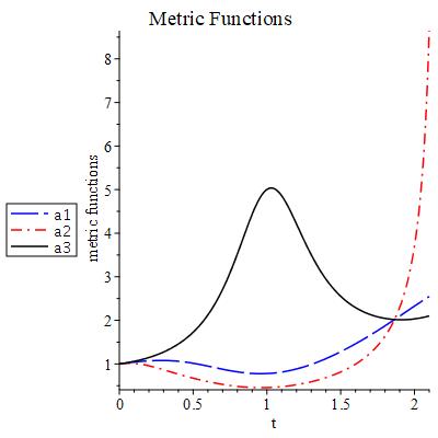
Figure 1: Evolution of the metric functions $a_{1}$, $a_{2}$ and $a_{3}$

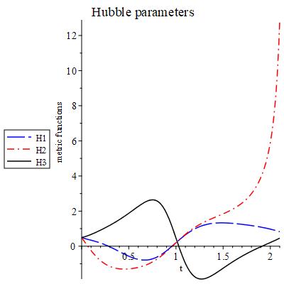
Figure 2: Evolution of the directional Hubble parameters $H_{1}$, $H_{2}$ and $H_{3}$

III conclusion

Within the scope of an anisotropic BI cosmological model we study the role of an interacting system of spinor and electromagnetic fields in the evolution of Universe. Earlier, it was shown that if a BI spacetime is filled with nonlinear spinor field, the nontrivial non-diagonal components of the EMT impose some severe relations both on spacetime geometry and spinor field. In particular, the spinor field becomes massless and liner in BI geometry. In this report it is shown that the introduction of electromagnetic field allows massive and nonlinear spinor field in BI spacetime. The corresponding system is obtained and solved numerically.

Funding: Not applicable

Institutional Review Board Statement: Not applicable

Informed Consent Statement: Not applicable

Acknowledgment:    This paper has been supported by the RUDN University Strategic Academic Leadership Program.

DAS: No datasets were generated or analyzed during the current study

Conflicts of Interest: No conflict of interests

References

• (1) Misner C.W. The isotropy of the universe. The Astrophysical Journal 151 , 431 (1968).
• (2) Hinsaw G. et. al. First Year Wilkinson Microwave Anisotropy Probe (WMAP) Observations: Angular Power Spectrum. Astrophysical Journal Supplimentary 148, 135 (2003).
• (3) Hinshaw G., et al. Five-Year Wilkinson Microwave Anisotropy Probe (WMAP) Observations: Data Processing, Sky Maps, and Basic Results. Astrophysical Journal Suppliment Series. 180, 225 (2009).
• (4) Saha B. and Shikin G.N Interacting Spinor and Scalar Fields in Bianchi Type $I$ Universe Filled with Perfect Fluid: Exact Self-consistent Solutions. General Relativity and Gravitation. 29(9), 1099 (1997);
DOI:10.1023/A%3A1018887024268
• (5) Saha B. and Shikin G.N. Nonlinear Spinor Field in Bianchi type-$I$ Universe filled with Perfect Fluid: Exact Self-consistent Solutions. Journal of Mathematical Physics 38(10), 5305 (1997);
DOI:10.1063/1.531944
• (6) Bijan Saha, Spinor field in Bianchi type-I Universe: regular solutions Phys. Rev. D 64, 123501 (2001);
DOI:10.1103/PhysRevD.64.123501
• (7) Armend$\acute{a}$riz-Pic$\acute{o}$n C., Greene P.B. Spinors, Inflation, and Non-Singular Cyclic Cosmologies. General Relativity and Gravitation. 35(9), 1637 (2003).
• (8) Saha B. and Boyadjiev T. Bianchi type-$I$ cosmology with scalar and spinor fields. Physical Review D. 69, 124010 (2004);
DOI:http://dx.doi.org/10.1103/PhysRevD.69.124010
• (9) Saha B. Nonlinear spinor field in Bianchi type-$I$ cosmology: inflation, isotropization, and late time acceleration. Physical Review D. 74, 124030 (2006);
DOI:http://dx.doi.org/10.1103/PhysRevD.74.124030
• (10) Fabbri L. Zero energy of plane-waves for ELKOs. General Relativity and Gravitation. 43, 1607 (2011).
• (11) Fabbri L. Conformal gravity with the most general ELKO matter. Physical Review D. 85, 047502 (2012).
• (12) Popławski N.J. Nonsingular, big-bounce cosmology from spinor-torsion coupling. Physical Review D. 85, 107502 (2012).
• (13) Bijan Saha, Spinor field nonlinearity and space-time geometry Physics of Particles and Nuclei 49(2), 146 (2018);
DOI: 10.1134/S1063779618020065
• (14) Bijan Saha, Nonlinear Spinor Fields in Bianchi type-I spacetime: Problems and Possibilities Astrophysics and Space Science 357, 28 (2015);
DOI: 10.1007/s10509-015-2291-x
• (15) Bijan Saha, Spinor field in FLRW cosmology Universe 9(5), 243 (2023);
DOI:10.3390/universe9050243
• (16) Rybakov Yu.P., Shikin G.N., Popov Yu.A. and Bijan Saha, Electromagnetic field with induced massive term: Case with scalar field Central European Journal of Physics 9(5), 1165 1172 (2011);
DOI: 10.2478/s11534-011-0033-4
• (17) Esteban M.J. and Georgiev V. Stationary solutions of the Maxwell-Dirac and the Klein-Gordan-Dirac equations, ICTP preprint IC/95/68
• (18) Das A. and Kay D., A class of exact plane-wave solutions of the Maxweel-Dirac equations J. Math. Phys. 30 (10) 2280 (1989)
• (19) Das A, An ongoing big bang model in the special relativistic Maxweel-Dirac equations J. Math. Phys. 37 (5) 2253 (1996)
• (20) Fierz M. Zur Fermischen Theorie des $\beta$-Zerfalls. Zeitschrift fur Physik A Hadrons and Nuclei 104, 553 (1937).