Breakdown of phonon band theory in MgO
Abstract
We present a series of detailed images of the distribution of kinetic energy among frequencies and wavevectors in the bulk of an MgO crystal as it is heated slowly until it melts. These spectra, which are Fourier transforms of mass-weighted velocity-velocity correlation functions calculated from accurate molecular dynamics (MD) simulations, provide a valuable perspective on the growth of thermal disorder in ionic crystals. We use them to explain why the most striking and rapidly-progressing departures from a band structure occur among longitudinal optical (LO) modes, which would be the least active modes at low temperature () if phonons did not interact. The degradation of the LO band begins, at low , as an anomalously-large broadening of modes near the center of the Brillouin zone (BZ), which gradually spreads towards the BZ boundary. The LO band all but vanishes before the crystal melts, and transverse optical (TO) modes’ spectral peaks become so broad that the TO branches no longer appear band-like. Acoustic bands remain relatively well defined until melting of the crystal manifests in the spectra as their sudden disappearance. We argue that, even at high , the long wavelength acoustic (LWA) phonons of an ionic crystal can remain partially immune to disorder generated by its LO phonons; whereas, even at low , its LO phonons can be strongly affected by LWA phonons. This is because LO displacements average out in much less than the period of an LWA phonon; whereas during each period of an LO phonon an LWA phonon appears as a quasistatic perturbation of the crystal, which warps the LO mode’s intrinsic electric field. LO phonons are highly sensitive to acoustic warping of their intrinsic fields because their frequencies depend strongly on them: They cause the large frequency difference between LO and TO bands known as LO-TO splitting. We calculate vibrational spectra from MD trajectories using a method that we show to be classically exact and therefore applicable, with equal validity, to any solid or liquid in any thermal or nonthermal state. By demonstrating its power and generality we show that it has become possible to go far beyond the reach of perturbation theories and mean-field theories in the study of vibrations in materials.
I Introduction
Band theories are theories of elementary excitations in crystals that are derived under the simplifying assumption that the elementary excitations are approximately independent of one another [3, 4, 5, 6]. For example, the band theory of electrons assumes that excited electronic states of a crystal are composed of weakly-interacting quasiparticles (QPs) [7], which are collective excitations of the electrons in which only one of the electrons plays a prominent role: A QP can roughly be described as a single electron whose electric field is screened, and whose energy and inertia are changed, by its many weak interactions with other electrons. When interactions between QPs are strong, they are not mutually independent and each one is not really a QP, but part of a more complex collective excitation in which multiple electrons play prominent roles [7]. The assumptions underpinning band theory are not valid for such excitations, and when they cause band theory to break down as an approximation, the electrons are said to be strongly correlated.
Similarly, the band theory of phonons assumes that the vibrational energy of a crystal can be approximated well by a sum of energies of individual phonons, or phonon quasiparticles, which are lattice waves with well defined frequencies and wavevectors. Phonon band theory breaks down when strong interactions between phonons with very different frequencies and/or wavevectors strongly correlate their motions, resulting in motion that cannot be characterized by a single wavevector and a single frequency, or even by a narrow range of wavevectors and a narrow range of frequencies.
Although strong electronic correlation has been the subject of intense study for decades, there have been few fundamental direct studies of strong phononic correlation [8, 9, 10, 11, 12]. One reason for this is the so-called terahertz gap, which is the region of the electromagnetic spectrum between about and where detectors, and intense continuous wave or pulsed sources, are either unavailable or not widely available [13, 14]. Another reason is that strong phononic correlation is difficult to observe experimentally because measured spectra tend to have low resolutions, making it difficult to detect when, or to what degree, the band theory of weakly interacting phonons has broken down.
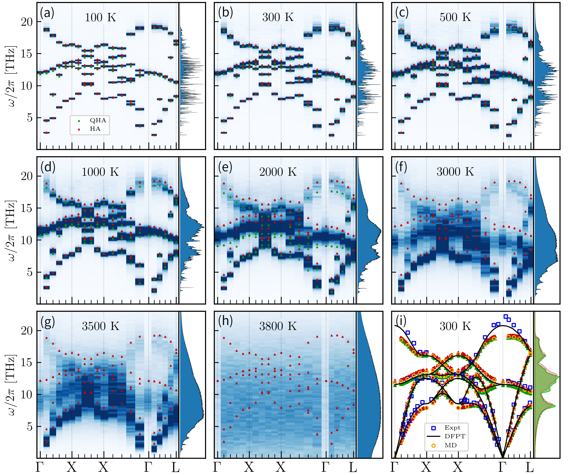
In this work we use atomistic simulations to study how the vibrational spectrum of MgO changes as its temperature () increases from , where band theory is accurate, to , where the crystal has melted and the spectrum has lost every semblance of a band structure. At each we calculate the distribution, , of kinetic energy in -space, or reciprocal spacetime, which are the terms we use to refer to the space of all wavevectors and frequencies. We present these spectra in Fig. 1, and analyze them and discuss them in detail in Sec. V.
Just as perturbation theories and mean-field approximations (e.g., Hartree-Fock) cannot accurately describe strongly-correlated electrons, mean-field approximations for phonons (so-called self-consistent phonon approximations [15, 16, 3, 4]) cannot accurately describe strongly-correlated phonons. Therefore mean-field based methods of calculating vibrational spectra [17, 18, 19, 20, 21] fail when phononic correlation is sufficiently strong, such as at high temperatures (), or in a liquid. However, the method we use to calculate spectra from our MD simulations is classically exact, which means that its accuracy is unaffected by the strength of phononic correlation.
Each distribution is the Fourier transform (FT), with respect to both space and time, of a mass-weighted velocity-velocity correlation function (VVCF) calculated from a molecular dynamics (MD) simulation at a different . The MD simulations were performed with a polarizable-ion force field whose parameters have been fit closely to the density functional theory (DFT) potential energy surface [22, 23].
It is common to Fourier transform velocity autocorrelation functions (VACFs) with respect to time to produce frequency-resolved spectra, such as those along the right-hand vertical edge of each panel in Fig. 1. However, wavevector-resolved spectra are relatively rare: They were calculated for a one dimensional material in Ref. 8, and more recently they have been calculated for three dimensional crystals using ab initio MD [24, 9, 11]. However, the computational expense of ab initio MD severely restricts the number of frequencies and wavevectors at which can be calculated. Therefore, so far, the resolutions of the spectra calculated by ab initio MD have been too low to see bands.
Force fields whose mathematical forms can mimic the electronic response to nuclear motion, and whose parameters are fit to enormous datasets calculated ab initio, provide a very useful balance of speed and accuracy [25, 22, 26, 27, 28, 29, 30, 31, 32]. As Fig. 1 illustrates, they allow accurate spectra to be calculated with resolutions that are high enough to see a crystal’s band structure. For example, Lahnsteiner and Bokdam [33] recently used them to calculate detailed spectra at two temperatures in order to extract phonon QP frequencies for use within band theory. Our purpose is very different.
The primary purpose of this work is to study strong phononic correlation. To this end, we have undertaken a systematic study of the strengthening of phononic correlation, and the consequent breakdown of band theory, as a crystal is heated.
We chose MgO for our study because it is a material whose vibrational properties are important in many contexts, from studies of seismic waves travelling through the Earth’s lower mantle, to its use as a thermal or electrical insulator, as a substrate for growing superconducting or ferroelectric perovskites, and in countless other important applications[2, 34, 23, 10, 35, 36]. As well as being a technologically-important material, MgO is one of the simplest oxides: It is a strongly ionic insulator with the same cubic crystal structure as rocksalt. For these reasons, it plays a similar representative role for oxides to that played by silicon for semiconductors: It is often the simplest setting in which properties or phenomena that are common to many oxides can be investigated. Several experimental and computational studies of phonon-phonon interactions in MgO and similar materials have recently been published [10, 37, 38, 12, 39]; therefore it is a natural and obvious starting point for investigating strong phononic correlation in oxides.
Calculations of detailed accurate spectra like those presented in Fig. 1 and by Lahnsteiner and Bokdam have been possible for a decade or more. One reason for their rarity may be that it is not commonly known that, within classical physics, the FT of the VVCF, , is exactly the distribution of kinetic energy in reciprocal spacetime: To our knowledge, all existing derivations and discussions of the theory rely on two simplifying assumptions: They assume that the crystal is at thermal equilibrium and that is low enough for the vibrational spectrum to be a band structure [40, 41]. After making these assumptions, the equipartition theorem is usually invoked to relate to the vibrational density of states (VDOS)[40, 41].
Lahnsteiner and Bokdam are among those who state that (our notation) is the wavevector-resolved VDOS, and they support this statement by citing Refs. 42, 43, 9, 24. This interpretation of , which can also be found in many other works [40, 41, 44, 45, 46, 47], is correct in the limit and under the simplifying assumptions that lead to band theory. It is also the appropriate interpretation of existing theory, because derivations such as those of Dove [40] and Lee et al. [41] only provide a clear physical interpretation of at thermal equilibrium in the limit.
However, it is shown in App. A and Ref. 48 that Fourier transforming the VVCF is a much more powerful and general method than it is currently believed to be: It is shown that is exactly the distribution of kinetic energy in reciprocal spacetime. Appendix A contains an illustrative proof of this result, for the case of a vibrating string. Therefore each of the spectra presented in Fig. 1 is exactly the distribution, among points in reciprocal spacetime, of the classical kinetic energy of the MD simulation from which it was calculated.
Furthermore, proving that is the kinetic energy distribution does not require any assumptions to be made about the statistical state or the structure of the material. It is a result that applies, with equal theoretical validity, to any crystalline or amorphous material, in any stationary or nonstationary state, regardless of the strength of the correlation between different vibrations and waves. This means that its range of possible applications is vast.
For example, it could be used to calculate the spectra of solids or liquids while they are being resonantly excited by THz radiation; or to study how spectra change during order-disorder phase transitions; or to investigate the relationships between structure, energetics, and diffusion in liquids. Using it may deepen our understanding of strongly correlated electronic systems, which are much harder to study computationally, by providing insight into aspects of strong correlation that are common to both phononic and electronic systems. It can also be used to assess the accuracies of approximate methods, such those based on perturbation theory, self-consistent mean-field methods, and methods that assume thermal equilibrium. As it is the only method that provides the exact classical spectrum, it is the method against which the accuracies of all other methods should be judged. A secondary purpose of this work is to demonstrate the power of this theoretical result and computational method.
By applying it to MgO we uncover a simple, strong, and general non-resonant mechanism by which the highest frequency optical modes of an ionic crystal can be disrupted by the lowest frequency acoustic modes, leading to the disintegration, or melting, of the optical bands. We call this mechanism acoustic warping of optical phonon fields. We also explain why, despite this mechanism causing longitudinal optical (LO) bands to melt, the acoustic bands responsible for their melting remain intact: It is because acoustic bands are adiabatically decoupled from LO phonons in the same way that heavy nuclei are adiabatically decoupled from electrons, despite pushing the electron density around as they move. Among many other analyses of the results presented in Fig. 1, we compare them to a second set of spectra (Fig. 3) which were calculated from MD simulations performed at the density. This allows us to discover which -induced changes to the spectrum can be explained by thermal expansion and which cannot. It also provides insight into the strengths and limitations of the quasiharmonic approximation [49, 40, 2].
In the next section we discuss the effects of on phonon band structures in general terms.
In Sec. III we explain our notation and some aspects of phonon theory that can be different when phonons are strongly correlated than they are at low where perturbation theories are applicable. For example, at high each mode is not Lorentzian, in general, and so the Lorentzian width is not a good measure of the degree to which has broadened it.
In Sec. IV we explain how we performed our simulations.
We begin Sec. V by discussing the most important limitations of our simulations. Then we begin discussing and numerically-analysing the spectra presented in Fig. 1 and Fig. 3. We focus our discussions and analyses on the most important and striking features of these spectra, and we include an explanation of the acoustic warping mechanism.
We summarize our conclusions in Sec. VI.
II Qualitative effects of temperature on band structures
In this section we discuss the qualitative effects of temperature on vibrational spectra. We begin with an illustration of a pertinent mathematical point.
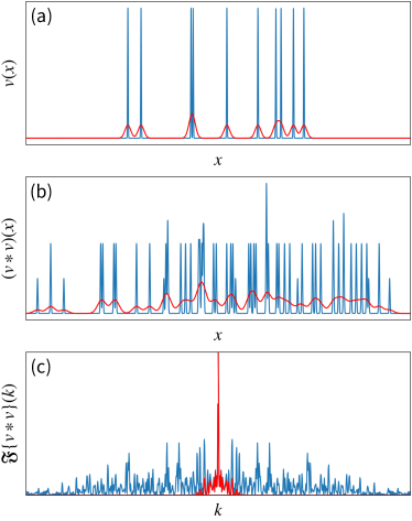
Figure 2(a) is a plot of two curves, each of which is the sum of ten randomly-positioned Gaussians. The only difference between the two curves is that the width of the Gaussians contributing to the red curve is a factor of ten larger than those contributing to the blue curve. The convolution of the red curve with itself and the convolution of the blue curve with itself are plotted in Fig. 2(b), and the Fourier transforms of these convolutions are plotted in Fig. 2(c).
It is well known that the more localized a smooth function is, the more delocalized its Fourier transform is [50]. These plots illustrate that the Fourier transform of the convolution of a smooth function with itself is more delocalized when the function is localized and vice-versa.
is the FT of the VVCF and the VVCF is the correlation of the spacetime distribution of -weighted atomic velocities with itself. The spacetime distribution of the atoms’ kinetic energy is more localized/delocalized when the spacetime distribution of their velocities are more localized/delocalized. Therefore Fig. 2 illustrates the fact that as kinetic energy becomes more localized in real spacetime it becomes more delocalized in reciprocal spacetime and vice versa. With this in mind, we now discuss the qualitative effects of temperature on vibrations in crystals.
II.1 Normal mode vibrations, phonon quasiparticles, and strong phononic correlation
Classically, and in the limit, the term phonon refers to an oscillation of one of a crystal’s normal modes of vibration, which are standing waves of the lattice that all of the crystal’s atoms participate in. Each normal mode is characterized by a single frequency () and a single wavevector () [48, 3, 5]. Therefore the energy of each normal mode vibration (NMV) can be regarded as localized at a point in reciprocal spacetime.
The amplitudes of NMVs vanish in the limit, making them perfectly harmonic and mutually noninteracting. Therefore the energy of each one is delocalized in spacetime. It is delocalized in space because every atom in the crystal participates in it and shares its energy. It is ‘delocalized’ in time in the sense that it is not transient: NMVs last forever in the limit because, without interactions, they cannot dissipate their energies; and they cannot disperse because each one is characterized by a single frequency and a single wavevector.
As well as being the limit in which kinetic energy is delocalized in spacetime and localized at a point in reciprocal spacetime, the limit is the limit in which atoms are strongly correlated and the limit in which phonons are uncorrelated: Each contribution to the atoms’ kinetic energy is a collective motion of all atoms, whereas each phonon possesses its own kinetic energy, which is independent of the energies of other phonons.
At finite , phonons’ amplitudes are finite, and they interact to some degree. When they interact, their motions become correlated and each one is no longer characterized by a single frequency and wavevector: it has become a superposition of NMVs with different frequencies and wavevectors. This interaction-induced mixing of frequencies and wavevectors is analogous to what happens when a pair of harmonic oscillators with frequencies and are coupled: The motion of each one becomes characterized by both frequencies; or equivalently, each one becomes an oscillation at frequency whose amplitude is modulated by an oscillation at frequency . When many oscillators are coupled strongly, the motion of each one becomes a superposition of oscillations at many different frequencies. Similarly, interactions cause each phonon’s energy to be distributed among the frequencies and wavevectors of all lattice waves contributing to its motion.
II.1.1 Phonon quasiparticles
At low finite each phonon is still mostly composed of a single NMV, but it contains small contributions to its motion from the other NMVs with which it interacts [3]. As increases and interactions strengthen the fraction of its kinetic energy contributed by the original NMV decreases and the fractions contributed by others increase. Therefore, as increases from the limit, each NMV’s kinetic energy spreads out from the point at which it was localized and becomes distributed among the frequencies and wavevectors of all of the NMVs with which it interacts.
At low the vibrational spectrum remains sharply peaked near the frequencies and wavevectors of the normal modes, but the peaks have finite widths. This means that each phonon contributing to each peak is a QP, i.e., a superposition of NMVs with very similar wavevectors and frequencies. Phonon QPs can dissipate their energies and disperse: their average lifetime is inversely proportional to the width of their spectral peak [3, 51]. Therefore, at low they are still reasonably long-lived excitations with reasonably well-defined frequencies and wavevectors, and one can think of each one as an NMV that is dressed by its interactions with other NMVs.
Interactions make the average frequency and wavevector of the QPs -dependent, and cause their spatial coherence (size) and temporal coherence (lifetime) to reduce as increases. The reduction in their sizes means that they are no longer collective motions of all atoms in the crystal. Therefore they are no longer standing waves, but travelling wave packets.
The kinetic energy spectrum, , is called a band structure at low because the set of points at which there are spectral peaks forms a set of three dimensional surfaces, or bands, in four-dimensional reciprocal spacetime. As each phonon becomes a mix of NMVs, these spectral peaks broaden and move, which causes the bands to blur, lose definition, and shift in frequency.
In quantum mechanics, the energies of NMVs and QPs are quantized and it is the quanta that are known as phonons. However, because most of our simulations and analyses are classical, we use the term phonon to refer to NMVs, in the limit, and to phonon QPs, at finite . A classical phonon is simply a vibration of the crystal whose wavevector and frequency are reasonably well defined, meaning that the distribution of its energy in reciprocal spacetime is sharply peaked, and most of its energy is localized in a small neighbourhood of its peak.
II.1.2 Strong phononic correlation
As increases further, sooner or later the -induced changes to the spectrum become more complex than a gradual shifting and symmetric broadening of QP peaks. Peaks may broaden so much that they vanish; one peak may become two peaks at very different frequencies and wavevectors; or the spectrum may deviate from a superposition of well-defined QP peaks in other ways, depending on the natures and strengths of the interactions. When the spectrum can no longer be approximated by a sum of reasonably-localized QP peaks, the quasiparticle approximation has broken down and the system can be regarded as strongly correlated.
When interactions between phonons are strong enough that the QP approximation has broken down, band theory also breaks down, because kinetic energy is so delocalized in reciprocal spacetime that it no longer forms bands.
For example, the energy of each oscillation in a liquid is localized in spacetime and delocalized in reciprocal spacetime. Oscillations are localized in space because spatial correlations are very short-ranged, which implies that only a small cluster of atoms participates in each one. They are localized in time because their strong coupling to other oscillatory and translational motions makes them transient: they have short lifetimes because they quickly disperse and/or dissipate their energies. Their short lifetimes can also be viewed as them morphing into other forms of motion, namely, diffusive motion or oscillations of different frequencies. For example, we can view the short lifetime of an oscillation of an atom as a consequence of the potential well in which it oscillates changing shape as neighbouring atoms move.
The eventual failure of band theory as increases is inevitable for every material because temperature generates disorder and because each point on a band represents a phonon with a different characteristic pattern of atomic displacements, or eigenvector, and with periodicities and in space and time, respectively. When such a vibration exists, it causes correlation between the velocity of an atom at time and the velocity of another atom, which is displaced from it by in the direction of , at time . Therefore, when there is a -induced reduction of the correlation length to less than , or of the correlation time to less than , the spectral intensity at point almost vanishes. When a particular mode or band loses all or most of its intensity in this way, we say that it has melted.
Band melting occurs gradually at most temperatures; and, as Fig. 1 illustrates, it occurs at different rates for different bands, because correlation lengths and times are different for motions along different eigenvectors, in general. The rate at which each band melts is determined by the natures and strengths of the interactions between the band’s phonons and other phonons. However, as Fig. 1(g) and Fig. 1(h) illustrate, when an acoustic band melts suddenly and completely, it means that the crystal has become structurally unstable and has undergone a phase transition. In some crystals, such as MgO, this does not occur until it becomes a liquid at the melting temperature of the crystal, . In others, such as ferroelectric BaTiO3 [52, 53, 54, 55], there are also one or more transitions between crystalline phases at ’s lower than .
III Elements of the theory of interacting phonons
In this section we present some elements of phonon theory that we will use in this work. A more complete account of this theory can be found in Ref. [48] and elsewhere in the literature [4, 3, 5].
III.1 Notation and definitions of key quantities
III.1.1 Structure of the crystal
We use to denote the number of atoms in each primitive cell, which is two in this case, and we denote the number of primitive cells in the crystal’s bulk by . We denote the primitive lattice vectors by and we identify primitive cells by their positions, , relative to an origin in the bulk of the crystal. These positions are lattice vectors, i.e., , where .
We use the compound index to identify the atom in primitive cell and we use to identify its lattice coordinate. We denote its displacement, at time , from its equilibrium position as . However, it is not very convenient to use vectors to specify the internal structure of each primitive cell. Instead, we specify it with a single vector , where , is the mass of the atom, and the set is a complete orthonormal basis of .
For simplicity, and despite its weighting, we will often refer to the vector and its time derivative as the displacement and velocity, respectively, of primitive cell . The kinetic energy of cell is .
III.1.2 Correlation functions and their Fourier transforms
The mass-weighted velocity-velocity correlation function (VVCF) is
| (1) |
where the average is performed over bulk cells, , and over times, . It is shown in Ref. [48] that the average kinetic energy per bulk unit cell is given by
| (2) |
where is the total kinetic energy of all bulk cells; is its time average; and is the discrete Fourier transform of with respect to both and . is the distribution, in reciprocal spacetime, of the time-average of the crystal’s kinetic energy per bulk primitive cell. As discussed in Sec. I, Eq. 2 is an exact expression, which is proved for the case of a vibrating string in Appendix A, and for a crystal in Ref. [48]. Theoretically, it is no less valid to apply it to a nonequilibrium liquid than it is to apply it to a low temperature crystal.
The first sum in Eq. 2 is over the set of all wavevectors within the first Brillouin zone, , that are compatible with the boundary conditions of the crystal. Within our treatment of the theory, wavevectors that differ by a reciprocal lattice vector, , are regarded as equivalent to the same wavevector in the first Brillouin zone, . If we wanted to distinguish between them, the right hand side of Eq. 2 would have the form , where is a function whose domain is the set of all wavevectors. However we are choosing to define and to restrict our attention to the finite set of wavevectors . This means that we do not explicitly distinguish between so-called Umklapp phonon interactions and normal interactions. This distinction is commonly made when treating interactions as scattering events, but in this work we emphasize the wave natures of phonons: Both in our classical simulations and, when is high enough, in a real crystal, phonons exchange energy with one another quasi-continuously.
The second sum in Eq. 2 is over all possible frequencies. This set is countable because if the total time for which a crystal is observed or simulated is , complete oscillations whose periods are longer than are not observed or simulated. Therefore oscillations with frequencies smaller than cannot contribute to . Furthermore, any two frequencies that do contribute to are only observably different if they differ by more than [48]. Therefore is only defined for , where is a nonnegative integer.
In a crystal, the limit of is a band structure. Therefore, when studying the breakdown of band theory, it is useful to decompose it into contributions from motions along each of the crystal’s normal mode eigenvectors. In Ref. [48] and many textbooks [3, 5, 4] it is shown that, deep within the bulk of a large crystal, each normal mode is associated with a particular wavevector, , and can be labelled by , where is the band index. At each wavevector the dynamical matrix has real eigenvectors, , where is a band index. We choose them to have unit norms and refer to them as the cell eigenvectors. At each , the set of cell eigenvectors, , is orthonormal () and is a complete basis of . The cell eigenvectors are -weighted polarization vectors [5, 4], but polarization vectors are not mutually orthogonal when there is more than one atomic species.
For any wavevector , we can express the identity in as and insert it into Eq. 1, to define the set of mode-projected correlation functions at wavevector ,
From this definition, and Eqs. 1 and 2, it follows that and , where denotes the discrete Fourier transform of with respect to and . In Sec. V we will pay particular attention to the LO mode and we will denote its cell eigenvector and mode-projected correlation function at by and , respectively.
When studying individual modes, we will make use of the normalized mode spectrum or mode distribution of mode , defined as
| (3) |
This function is the distribution among frequencies of the energy of oscillatory motion in the bulk of the crystal along the eigenvector of normal mode .
When studying the spectrum as a whole, calculating from is equivalent to calculating from for each mode and summing over all modes. Therefore, the spectra plotted in Fig. 1 are plots of
| (4) |
At thermal equilibrium, the equipartition theorem states that the expectation value of the kinetic energy of each mode is . Therefore, if the spectra plotted in Fig. 1 were converged fully, the denominators of both expressions in Eq. 4 would be . However, regardless of whether or not is converged with respect to simulation time or supercell size, it is the exact distribution, among wavevectors and frequencies, of the average kinetic energy per primitive cell of the trajectory from which the VVCF was calculated.
III.2 Energy expanded in mode coordinates
The displacement of the crystal from equilibrium can be expessed as a sum of displacements along its normal mode eigenvectors. We denote the frequency of mode by , and the projection of the crystal’s displacement from equilibrium at time onto its normalized eigenvector by , which we refer to as its mode coordinate. The total energy of the crystal, as a function of the mode coordinates and their time derivatives, can be expressed as
| (5) |
where is the potential energy of the static lattice in the limit (excluding zero point energy); vanishes because the first partial derivatives of the potential energy vanish at equilibrium; the kinetic energy is ; the harmonic term of the potential energy is , and , where , denotes an anharmonic term of order .
III.3 Difference between the kinetic energy distribution and the VDOS
As discussed in Sec. I, is usually interpreted as being proportional to the VDOS at low [42, 40, 41, 43, 44, 45, 46, 47]. However, this interpretation is only valid under the simplifying assumptions that there are as many vibrational states as there are degrees of freedom and that the crystal is at thermal equilibrium. When these assumptions are not valid, the kinetic energy distribution is a very different quantity to the VDOS because there is kinetic energy at if one or more waves exist with wavevector and frequency ; and because the most general and rigorous treatments of phonon theory do not place any restrictions on which waves may exist at finite .
Therefore, let us assume that one of the defining characteristics of each ‘state’ that contributes to the VDOS is that it is independent, or approximately independent in the temperature range of interest, of the amount of kinetic energy that ‘occupies’ it. Then, the only viable definition of the set of all states is this one: at every point , there are exactly as many occupiable vibrational states as there are degrees of freedom in a primitive unit cell.
For example, in our MD simulations, there could be kinetic energy at any point on a four-dimensional lattice in reciprocal spacetime whose lattice spacing along the frequency axis is inversely proportional to the total simulation time and whose lattice spacings along the three wavevector axes are inversely proportional to the linear dimensions of the simulation supercell. Therefore the VDOS of the simulated system is a uniform distribution with exactly states per point of the lattice that our simulation samples.
To illustrate that this is the case, note that each spectrum in Fig. 1 is pixelated. The 2-d lattice consisting of points at the centers of the pixels is a 2-d representation of the 4-d VDOS. Therefore there are six states at the center of every pixel, including at the centers of pixels that are white. Pixels are white when none of the states at their centers are ‘occupied’ by kinetic energy. However, the fact that they are not occupied does not mean that they are not occupiable, and some of them can be seen to turn blue at high (e.g., when the crystal melts), indicating that they have become ‘occupied’ by some of the kinetic energy.
III.4 Independent-phonon approximations
In the bottom right panel of Fig. 1 we compare the band structures measured experimentally [1] with those that we have calculated using three different (quasi)independent-phonon approximations; namely, the harmonic approximation (HA), the quasiharmonic approximation (QHA), and the quasiparticle approximation (QPA).
In the HA, all cubic and higher-order anharmonic terms in the potential energy are discarded, which is tantamount to assuming that there is no interaction between different modes, and the Helmholtz free energy, , can be approximated as [3]
| (6) |
where is the Boltzmann constant, and the ‘’ subscript on indicates that it is the free energy within the harmonic approximation, . Notice that only depends on via the second term in the summation over modes, but that it depends on via the cohesive energy, , and the mode frequencies, .
When the third term vanishes in the limit, it becomes . However, if phonons are treated classically, as in our MD simulations, the zero-point energy term does not exist and we simply have . Therefore the limits of the mode frequencies calculated within the QHA and the QPA are different. They are the harmonic frequencies calculated at the volumes that minimise and , respectively.
III.4.1 Quasiharmonic approximation (QHA)
One of the most important ways in which the vibrational spectra of materials change with is via thermal expansion: Lengthened bonds tend to be weakened bonds, and weakened bonds vibrate with lower frequencies. Therefore thermal expansion tends to lower phonon frequencies, on average. Within perturbation theory, this effect is often modelled using the QHA, which entails calculating the normal mode frequencies at a range of volumes and using them in Eq. III.4 to calculate . The volume that minimizes is then found and treated as the equilibrium volume at temperature , and the normal mode frequencies at this volume are used to calculate thermodynamic properties from . In the most commonly used form of the QHA [2, 12], which is the form that we use, the dependence of on is ignored when taking derivatives of with respect to .
The QHA approximates the shift of phonon frequencies by thermal expansion, which is often the largest effect of anharmonicity on vibrational spectra at low . However it does not explicitly describe any phonon-phonon interactions and therefore cannot describe other important effects of anharmonicity, such as the broadening of peaks in the mode spectra, , as increases.
III.4.2 Quasiparticle approximation (QPA)
At very high , such as in the liquid, each mode spectrum is not strongly peaked at any particular frequency. However, in the limit, it becomes the delta function and at small finite values of it is a sharply-peaked distribution of finite width.
We denote the peak position of mode distribution at temperature and volume by
| (7) |
where is the harmonic frequency in the limit at volume and is a finite- correction, which does not depend on to leading order in anharmonicity [3]. At constant pressure, is determined by ; therefore we can write . The shifted frequencies, , are the QP frequencies. They can be used to calculate thermodynamic properties in manner that is similar, but not identical for all properties [3], to how harmonic phonon frequencies are used.
III.5 Band broadening
As discussed, is a delta function in the limit and, as increases from this limit, its first effects on are to broaden it and to shift it in frequency.
If phonons were independent entities that are created and annihilated in sudden random occurrences, which might be described as collisions or scattering events, then, at thermal equilibrium, the average rate at which phonons of each mode were created would be equal to the rate at which they were annihilated; and annihilation events would be Poisson distributed. It follows that phonon lifetimes would be exponentially distributed and that each mode correlation function would decay exponentially as a function of time [56].
In the limit, is sinusoidal in both and . Therefore, when annihilation events are Poisson distributed at finite , it becomes an exponentially-decaying sinusoid, , and its Fourier transform, , is Lorentzian. Therefore is also Lorentzian, i.e.,
| (8) |
where is a constant, is the QP frequency, is the full-width at half maximum (FWHM) of the Lorentzian and is the rate of exponential decay of the energy of a phonon QP of mode . Therefore, when can be fit closely by a Lorentzian, quantifies the degree to which it has been broadened by temperature.
On the other hand, when phonons are treated as lattice waves that continuously exchange energy, each -broadened spectrum, , is only Lorentzian at very low when it is a very narrow peak. At higher , its shape is determined by the relative strengths of its couplings to other modes.
At any finite , if is sufficiently small we can interpret as the probability that the frequency of the oscillation along the eigenvector of mode at a randomly chosen time is between and . We could also interpret it as the probability that the duration of the complete oscillation that begins at a randomly chosen time is between and . Therefore we can use Shannon’s theorem to quantify the effects of on mode by quantifying the degree of uncertainty in its frequency. As Shannon demonstrated in the context of signal processing [57], the correct way to quantify this uncertainty is by the mode entropy,
| (9) |
For a given variance of , the shape that maximises is a Gaussian.
Although using the mode entropy, , to quantify the degree of broadening is both more general, and better justified theoretically, than fitting to a Lorentzian, the latter is more common in the experimental literature. Therefore we calculated both and .
III.6 Anharmonicity
Phonon-phonon interactions can be considered explicitly in perturbation theory by including cubic and higher-order terms in the truncated Taylor expansion of the potential energy. However, at any chosen order, phonon perturbation theory fails when is high enough. Furthermore, although in the limit each individual term of order contributing to in Eq. 5 is larger than each individual term of a higher order contributing to , there are more nonvanishing terms than terms, in general. For example, as Ashcroft and Mermin [5] point out, the number of quartic terms that do not vanish by symmetry can be much larger than the number of nonvanishing cubic terms. As a result, even at low , the magnitude of can be comparable to, or greater than, the magnitude of . They also point out that a crystal would not be stable if its Hamiltonian was ; must be added for stability.
The fact that is not necessarily greater than when makes truncation of Eq. 5, which is a necessary step in any application of perturbation theory to real materials at finite , formally unjustified. The method based on correlation functions that we use is free of such complications. Therefore it is a useful tool for checking when/whether perturbation theories are applicable and for assessing their accuracies.
A related limitation of perturbation theory is that it is often necessary to calculate and analyse so many phonon interaction terms that the underlying physics can become lost in the clutter. For example, the anomalous broadening of the longitudinal optical (LO) mode near the BZ center evident in Fig. 1 has been studied by perturbation theory and explained, in part, as a consequence of the band structure [38, 12]: the number of nonvanishing contributions to that involve the LO mode near is very high because of the locations in -space of the other modes.
This is an important observation, which is likely to be part of a complete explanation, but on its own it is not a complete and satisfactory explanation. Explaining one feature of a spectrum as being a consequence of its other features is not satisfactory because the spectrum as a whole is not self-determined: It is determined by interactions between waves passing through a lattice of ions. A more complete explanation of a spectral feature would explain it in terms of the motions of waves and ions.
It is also important to note that, when treating phonon at finite as a QP whose dynamics are damped with a decay constant , the contribution of modes and to the value of could be negligible despite the magnitude of the term in proportional to being very large. It is not enough that modes and exchange a lot of energy with mode : they must do so irreversibly. This means that if they absorb some of mode ’s energy, they must dissipate it, by coupling to more modes, before it has time to return to mode . For example, when two harmonic oscillators are coupled, their combined energy oscillates back and forth between them. There are times when one of them has all of the energy and times when the other has it all. Therefore, in a thermal population of phonons, it is not necessarily possible to calculate decay constants accurately as sums of few-phonon contributions.
Reference [8] provides an illustration of this point. It was found that when two coaxial nanotubes are in relative sliding motion, phonons are resonantly excited at every sliding velocity. However, it is only at a small number of velocities that these resonances manifest as a strong friction force that slow the sliding motion down. The energy exchange between the mechanical motion of the tubes and most of the resonantly-excited phonons is equitable. High friction only occurs at velocities for which the resonantly-excited phonons dissipate the energy they absorb from the sliding motion more quickly than they return it to that motion.
Irreversible dissipation of energy always requires the participation of very large numbers of modes. Therefore because, in practice, perturbation theories are limited to considering few-phonon processes, they have a fundamental limitation that the MD-based method used here and in Ref. [8] does not share.
The purpose of this section is not to denigrate phonon perturbation theories. It is to point out that both perturbation theories and the correlation function approach to calculating spectra are limited, but in different ways; therefore they complement one another. We have used harmonic phonon theory extensively to analyse our spectra, and it is likely that we would have learned much more with the help of anharmonic terms.
In Sec. V.2.3 we provide a simple explanation of the anomalous LO broadening, in terms of ions and waves, and without referring to any other feature specific to the vibrational spectrum of MgO and the other similar materials in which anomalous LO broadening has also been observed [58, 59, 60, 61, 62, 63, 64, 65, 66, 67].
We suggest that the acoustic warping mechanism we propose in Sec. V.2.3 modulates the frequencies of LO modes, and therefore the expectation values of their occupation numbers. At thermal equilibrium, a mode whose frequency is fixed exchanges energy with other modes equitably: its net rate of energy exchange with other modes vanishes. However, because the LO mode’s frequency is changing, the expectation value, , of its occupation number is changing, and this might make its net rate of energy exchange with other modes finite. This net exchange of energy may happen quickly (e.g., for the reasons explained by Giura et al. [38]) relative to the period of the acoustic mode modulating , and so it may contribute significantly to the degradation of lower-frequency bands.
IV Simulation details
IV.1 Atomistic force field
Atomistic molecular dynamics (MD) and lattice dynamics (LD) simulations were performed using a polarizable-ion potential of the form described in Refs. [25, 28, 68], and used to study the pressure dependence of the melting temperature of MgO in Ref. [23].
Our method of force field construction [22] is a form of supervised machine learning [69, 32], albeit one that predates the widespread adoption of the term machine-learning in this context. However, the interactions described by most machine learning force fields are near-sighted 69, whereas a realistic description of long-ranged Coulomb interactions is essential when studying zone center LO phonons. Therefore, we did not impose any accuracy-lowering near-sightedness constraint on the mathematical form of our potential.
Our force field’s parameters were fit to an effectively-infinite dataset of forces, energy differences and stress tensors from density functional theory (DFT) calculations using the PBEsol functional [70]. As discussed in Refs. [71, 72] and [22], describing the polarizability of oxide anions, either implicitly or explicitly, is necessary for an atomistic model of an oxide to accurately describe the long range fields that are intrinsic to LO phonons. However, cations’ electrons tend to be much more tightly bound and we did not find a significant improvement in the fit to DFT data when Mg cations were polarizable, so we assigned a polarizability of zero to them.
The mathematical form of the potential and the values of the parameters used are quoted in Appendix B. In brief, it is the sum of a pairwise interaction, comprising a Morse potential and a Coulomb interaction, and the Coulomb interactions between dipoles induced on oxygen anions and the charges and induced dipoles of other ions. The dipole moment of the oxygen anion is expressed as , where is a short-range (SR) contribution caused by asymmetry of the space in which its electron cloud is confined by its six cation neighbours, and is the dipole moment induced by the local electric field () from the charges and dipole moments of all other ions. At each step of the MD simulation, we first use the method of Wilson and Madden to calculate [73] as a function of the distances of ion to neighbouring ions. Then we iterate the coupled equations (one for each anion) to self consistency in the set of all dipole moments , where oxygen’s polarizability, , is among the parameters fit to DFT data. Finally, we calculate the Coulomb energy of interaction between each dipole moment and the charges and dipole moments of all other ions.
IV.2 Molecular dynamics
We simulate under periodic boundary conditions and our supercell is a repetition of the two-atom rhombohedral primitive unit cell. We use velocity rescaling, followed by of equilibration in the ensemble, to prepare for production runs at each temperature, . Our production runs of are also performed in the ensemble and the reported values of are calculated from the average kinetic energy of the production run. We use a time step of and sample positions and velocities every ten steps for later analysis. We chose to perform our MD simulations at constant volume, but with , instead of at a fixed average pressure and a variable volume. Although the magnitudes of the fluctuations of each primitive cell’s volume would be reduced, to some degree, by simulating with the supercell volume fixed, this was deemed preferable to polluting our spectra with unphysical artefacts of an MD barostat.
We performed one set of simulations with the volume at each chosen such that the average pressure () in the crystal at that is close to zero. The averages of in these simulations were , , , , , , , and . The pressure is large in the highest temperature simulation because the crystal has melted and we did not repeat the simulation with the volume adjusted for the liquid phase. At all lower temperatures the simulation cell is crystalline and the maximum estimated percentage error in the simulated volume is , where is its bulk modulus under ambient conditions [2, 74].
Another set of MD simulations at approximately the same values of
was performed with the volume fixed at its value in the low temperature
limit, i.e., at the value obtained by minimizing the enthalpy with respect to
atomic positions and the lattice parameter.
The averages of in this set of simulations were
,
,
,
,
,
,
and
.
IV.2.1 Correlation functions and their Fourier transforms
We used fast Fourier transforms (FFTs) to compute vibrational spectra from correlation functions. We calculated spatial correlations up to the maximum distance possible with our supercell, which is , where is the primitive lattice parameter. We used the entire production run trajectory of length to calculate temporal correlations. The resolutions, and , with which spectra can be calculated as functions of wavevector () and frequency (), respectively, are determined by the sizes of the domains in space () and time (), respectively, on which the correlation functions are calculated. With our supercell we are able to sample five commensurate -points between () and (), where is a commensurate -point if waves with wavevector respect the periodic boundary conditions, i.e., if , where each is an integer, is parallel to the supercell lattice vector, and if the length of that lattice vector is an integer multiple of . The frequency resolution of our raw spectra is , but we smooth them along the frequency axis by convolving them with Gaussians of standard deviation , for the spectra at , and for the spectra at .
IV.3 Lattice dynamics
To calculate the phonon band structure within the harmonic approximation, we find the equilibrium () structure of the supercell and then calculate the dynamical matrix from finite differences of forces after displacing atoms slightly from equilibrium. To avoid artefacts of interpolation, we only plot the frequencies at commensurate -points, but we increase their density in reciprocal space by calculating phonon spectra on supercells for .
As discussed in Sec. III.4.1, the QHA simply amounts to calculating the phonon band structure at the equilibrium volume for the given temperature, , rather than at the equilibrium volume of the limit. The equilibrium volume at temperature is the volume that minimizes the free energy; but we cannot calculate the free energy easily, precisely, or accurately due to important contributions to it from improbable microstates. Improbable microstates are unlikely to be sampled in an MD simulation and if, by chance, they did occur, they would be oversampled. However we can calculate the free energy under the simplistic assumptions that phonons do not interact with one another and that the vibrational energy is distributed among the phonon bands according to the Bose-Einstein distribution. Therefore, when we apply the QHA we assume that band theory is a good approximation and we calculate the phonon bands as a function of volume. We use these frequencies in Eq. III.4, which is exact in the limit where band theory is exact, to find the volume that minimizes .
We calculated for a range of volumes corresponding to a set of lattice parameters with uniform spacing , and we interpolated between these values with cubic splines. To calculate the phonon frequencies at each volume we use a supercell to calculate the dynamical matrix at each in the commensurate set from finite differences of forces. When calculating from Eq. III.4, the sum over is a sum over the set of commensurate -points.
V Results
| 500 K | 1000 K | 2000 K | 3000 K | 3500 K | ||||
|---|---|---|---|---|---|---|---|---|
| - | - | |||||||
We presented the central result of this work in Fig. 1, which contains eight kinetic energy spectra that show how thermal disorder degrades the optical bands of MgO. Before analysing and discussing these spectra, we discuss some limitations of our calculations that should be borne in mind while interpreting them.
V.1 Sources of inaccuracy and imprecision
The first limitation is our use of approximate interatomic forces. The accuracy with which our force field calculates phonon frequencies at is evident in the bottom-right panel of Fig. 1, where we compare with measured phonon frequencies and with those calculated ab initio with DFPT. The underestimation of LO frequencies at small wavevectors is common for force fields of this kind [75, 22, 68], and has been discussed in Ref. 68. It is likely to be caused by the induced dipoles of the force field overscreening the long wavelength electric fields that LO phonons create, and which increase the frequencies of LO phonons relative to transverse optical (TO) phonons.
The accuracy with which our force field describes thermal expansion is evident in Table 1. Its accuracy for other properties and at higher is more difficult to assess because we have neither more accurate calculations nor experimental measurements to compare with. However, force fields of the same mathematical form, and parameterized in the same way, were used in Refs. 22 and 23 and shown to predict the pressure dependences of the crystal’s volume () and melting temperature () accurately, and to produce pair correlation functions for molten MgO in perfect agreement with those produced by ab initio MD simulations.
To parameterize the force field used in this work we fit to DFT data calculated with the PBEsol functional [70], which tends to be more accurate than the local density approximation used in Refs. 22 and 23. Furthermore, we fit the parameters to DFT calculations of crystalline MgO, whereas those used in Refs. 22 and 23 were required to describe MgO in both molten and crystalline forms, which meant compromising on the accuracy with which each phase was described.
Based on the tests performed here and in those previous works we suggest that, at worst, our force field should be regarded as describing an MgO-like material. We further suggest that some of the gross features of the -dependence of the spectra calculated with it, including those that we have selected for discussion below, are caused by simple physical mechanisms that would occur in other ionic crystals and therefore might manifest in their vibrational spectra.
A second limitation of our calculations is that our MD simulations are classical simulations. Therefore their accuracy at low is questionable. However, when is comparable to, or greater than, the Debye temperature (), which is the range of most interest for studying the breakdown of band theory, this approximation should not affect our results significantly. Furthermore, we will show in Sec. V.3 that the heat capacities calculated from the quasiparticle energies extracted from MD simulations are in very good agreement with measurements at all values of between and .
We regard our use of a supercell of finite size in our MD simulations as by far the most important source of inaccuracy and imprecision in the kinetic energy spectra presented. It means that the only lattice waves present our MD simulations were those whose wavevectors are commensurate with the supercell. Our use of a supercell means that the longest finite wavelength among the phonons in our simulation was only ten times the length of a primitive lattice vector. To make clear that we only calculate spectra at a finite number of points in -space, we have pixelated the spectra, with one pixel centered at each commensurate -point. However, the absence of any vibrations at incommensurate -points would change how energy is distributed among the commensurate set of points. For example, in a real crystal there would be far more channels (modes) through which energy and momenta could be exchanged.
V.2 Deviations of finite- spectra from band structures
Let us now begin discussing Fig. 1, which compares the full -resolved kinetic energy spectra, , from our MD simulations at different values of , after each one has been normalized so that it integrates to one.
As mentioned in Sec. III.1.2, the equipartition theorem implies that if the spectra were converged fully with respect to simulation time, this normalization would be equivalent to dividing each one by the same constant and by . Regions of high and low energy density are coloured dark blue and white, respectively, with the same colour scale used at each . For comparison, the band structure and the finite- QHA band structures are plotted over the full spectrum with red and green triangles, respectively.
The spectra show a progressive transition between two limits of : Phonon bands are well defined at low , whereas at very high they are much less well defined or not defined. At the phonon dispersions do not differ substantially from the bands calculated within the HA: All of the vibrational energy is localized near the normal mode points, , and the widths of the peaks at these points are small. At , on the other hand, the phonon bands have vanished and the spectrum is much more uniform and has little observable structure. This is because the crystal has melted and because spatial and temporal correlations are very short in a liquid. Therefore the phonon assumption of atoms moving collectively as waves has broken down completely.
The spectra at other s show various stages of the progression between the low- limit, in which atoms move as lattice waves with well defined frequencies and wavevectors, and the liquid, in which each atom moves independently of all other atoms, except those closest to it.
Note that MgO melts at [23, 36], but it is well known that, by imposing a degree of long range order, the periodic boundary conditions used in MD simulations can prevent melting until is significantly larger than [76]. Therefore, the spectrum in Fig. 1 should be regarded as the spectrum of a superheated MgO crystal.
V.2.1 Selected features of the kinetic energy spectra
There is a lot of complexity in the -dependence of the full spectrum (Fig. 1) and a much more extensive and detailed study would be required to explain it all. Therefore we provide the data used to produce Fig. 1 as Supplementary Material so that others may analyze it further [77]. We focus our attention on two important gross features of the spectrum’s -dependence, and on one striking specific feature.
The first gross feature is that all phonons shift to lower frequencies as increases. Most of this softening can be attributed to the weakening of bonds by thermal expansion. We will discuss this in more detail in Sec. V.3.
The second gross feature is that optical bands, and particularly LO bands, lose definition much more rapidly with increasing than acoustic bands; and zone center modes (, ) lose definition much more rapidly than zone boundary modes. Much of the intensity seen at high frequencies and small wavevectors at low gradually moves towards lower frequencies and larger wavevectors as increases. This is easiest to see along the wavevector paths and , which are straight line segments connecting the zone center () to the high symmetry points and on the zone boundary. We will denote the wavevectors at and by and , respectively.
When analysing spectra, we will ignore the point itself, which does not represent the limit , but the point : The intensity at in Fig. 1 is the kinetic energy of rigid relative motion of the Mg and O sublattices in our simulations, which does not interest us. However, note the disappearance, at high , of most of the intensity at optical frequencies and at wavevectors of , , , and , which are the smallest finite wavevectors along these paths that our simulation supercell can accommodate. The redistribution of intensity away from high frequencies at these wavevectors means that, at very high , little of the crystal’s kinetic energy exists as coherent optical waves whose wavelengths are greater than about five or ten lattice spacings. The TO branches retain significant amounts of energy at these wavelengths, but the LO bands have almost vanished. As discussed in Sec. II, much of this is a manifestation of thermal disorder reducing the correlation lengths and times of collective motions along the cell eigenvectors of the affected modes, causing them to become less wavelike and more localized in spacetime.
While this is happening to optical bands at small wavevectors, the acoustic branches of the spectrum remain relatively robust. Melting manifests in the spectra as the sudden total loss of definition and integrity of the acoustic bands between and .
The broadening of bands does not necessarily mean that the waves contributing to the band are less coherent. A band of finite width can broaden further without the phonons’ coherence lengths and lifetimes reducing further if the broadening is caused by a very slow modulation of the properties of the underlying lattice. As we discuss further below, the frequency and/or wavevector of an optical mode could be modulated by an acoustic phonon whose period and wavelength are much larger than the optical phonons’ coherence length and lifetime, respectively.
The specific striking feature of the spectra that we have chosen to discuss is that the loss of definition of the optical modes appears to begin with an anomalously-large broadening of the LO modes nearest to , and to spread out from these -points as increases. The broadening of these modes is even visible at , which is the lowest at which we calculated the full spectrum, and it occurs for the LO phonons at all wavevectors near , regardless of their directions.
We are not the first to observe the anomalous LO linewidth at low in MgO [38, 12]; and similar features have been observed experimentally in similar materials since the 1960s, and more recently in calculated spectra [58, 59, 60, 61, 62, 63, 64, 65, 66, 67]. However, we have not found other studies that show how it evolves as the crystal is heated to a very high , and that it marks the beginning of the gradual melting of the entire LO band. When the set of spectra in Fig. 1 are examined collectively, the melting of the LO band may be the most noticeable feature of the spectrum’s -dependence between and .
Because the LO band melts gradually and systematically from its apparent origin, at low , as a localized anomaly near the BZ center, and because similar anomalies have been observed in other materials, we believe that its primary cause is a simple and general physical mechanism, which we refer to as acoustic warping of optical phonon fields. The effects of this mechanism on vibrational spectra would be particular pronounced in crystals with large LO-TO splittings, such as strongly ionic materials with the rocksalt crystal structure. We explain it in the sections that follow.
We begin by suggesting an explanation for why strong coupling between low frequency acoustic phonons and optical phonons would melt optical bands much faster than acoustic bands. Then we explain the acoustic warping mechanism, why it would cause LO bands to melt, and why this melting would begin near the BZ center before gradually progressing outwards, until the only LO modes that remain are those at the BZ boundary.
V.2.2 Separation of optical and acoustic timescales in the long wavelength limit
The acoustic branches can be thought of as a skeleton on which the optical branches ‘hang’, because spatially-coherent countermotion of cations and anions about a reference structure would not happen unless the reference structure was itself spatially coherent. For example, consider the projection, of the displacement of cell onto the cell eigenvector of the LO mode at . When regarded as a function of , this projection is very unlikely to have order on length scale if the crystal does not have order on length scale . Crystalline order is gradually lost as increases, and this manifests as a gradual reduction of the correlation lengths and times of this projection, i.e., as an increase in the rate of decay of as a function of at fixed and as a function of at fixed finite .
The energy cost of acoustic distortions protects long range order in the time average of the crystal’s structure. However, if is small, the crystal having long range order when averaged over several periods of a long-wavelength acoustic (LWA) mode is not sufficient to protect long range order in . It is insufficient because the periods (frequencies) of zone center LO modes are much shorter (higher) than those of LWA modes. Therefore long range order of as a function of relies, not on the degree to which the time average of LWA mode displacements preserve crystalline order (i.e., vanish), but on the degree to which they preserve it on timescales much shorter than LWA mode periods. Long range order of the optical branches requires the amplitudes of LWA modes to be small, not their time-averaged displacements.
The converse is not true and, in either the limit of large LO frequency, , or the limit of small LWA frequency, , the coupling between LWA and LO modes is almost unidirectional: LO vibrations are highly sensitive to LWA mode displacements, whereas LWA vibrations are much less sensitive to LO mode displacements. The reason for the high sensitivity of LO phonons to LWA phonons will be discussed in Sec. V.2.3.
LWA phonons are relatively insensitive to LO phonons because an LO mode’s period, , is so short that LO displacements average to zero in much less than the period, , of an LWA phonon. Therefore the forces they exert on an LWA mode cancel one another before the LWA mode has had time to respond to them. On the length and time scales relevant to the lowest-frequency LWA modes of a macroscopic crystal, the crystal is a continuum and the LWA modes do not see optical mode disorder directly, but experience its effects indirectly through the -dependence of the crystal’s elastic constants.
This partial decoupling of a slow-moving degree of freedom from a much faster one is known as adiabatic decoupling [78, 79, 80, 81, 82]. It is exploited by the Born-Oppenheimer approximation: An excellent approximation to the force exerted on a heavy nucleus by electrons is calculable from the electron density, which can loosely be thought of as the time average of the electrons’ positions.
Adiabatic decoupling does not mean that the LWA modes do not exchange energy with the optical modes. It means that their energy exchange is so rapid that they barely notice. The net energy exchange in a time can be very large if , but is likely to be negligible if , because its average over one complete LO period is small and its average over many complete periods is even smaller. Optical mode disorder changes so quickly that every complete LWA oscillation occurs in the presence of an almost equivalent background of optical displacements, whereas LWA disorder changes so slowly that every complete LO oscillation occurs in the presence of a unique and inequivalent background of LWA displacements.
Therefore it is approximately true that LWA phonons only experience the many rapidly-changing LO displacements as a slight dressing, which changes their frequencies very little. Nevertheless, and at the same time, if there exists an effective LWA-LO coupling mechanism, the frequencies and coherence lengths and times of LO phonons are strongly influenced by whatever LWA displacements exist during their lifetimes.
Of course, the adiabatic decoupling picture, in which optical modes see ‘frozen’ acoustic modes and acoustic modes do not see optical modes because the time averages of their displacements vanish, is very much an idealized limiting case. Adiabatic decoupling of acoustic modes from optical modes becomes a perfect decoupling in the limit, but is likely to be far from perfect at the smallest finite wavevectors present in our simulations. Clearly this picture would not apply to the transverse acoustic (TA) and TO modes in the regions of the BZ where they occupy the same small frequency window between about and . However, it does seem to explain why the lowest-frequency acoustic modes are broadened less than the highest-frequency optical modes.
As increases from the limit, it is the LWA modes that are first to become active, because they are lowest in energy. Therefore, there may be a common explanation for why the LO band is the first to melt, or partially melt, for why zone center modes melt before zone boundary modes, and for why acoustic bands are degraded less at the highest ’s than optical bands: Acoustic modes are degraded less because of the partial immunity to optical disorder that adiabatic decoupling affords them. LO modes are not protected by adiabatic decoupling and, as we now explain, there is a very simple and effective mechanism by which they can be disrupted, and their frequencies changed, by acoustic disorder; or even by a single quasistatic acoustic perturbation of the crystal.
V.2.3 Acoustic warping of the LO electric field
By modulating the relative displacements of cations and anions, an LO wave of wavevector creates regions of excess charge at its nodes, from which emanates an electric field, , of the same wavelength, . This field, which we referred to as the LO mode’s intrinsic field above, opposes the LO wave’s motion, thereby increasing its frequency, [83, 5].
One way to understand the origin of is to consider the case in which is orders of magnitude larger than a primitive lattice spacing; and to imagine partitioning the crystal into primitive unit cells of dipole moment , whose volume we will treat as infinitesimal.
If the LO mode at wavevector becomes active, it modulates along an axis parallel to by modulating the displacements of Mg cations from the O anions with which they share a primitive cell. On length scale , we can define a local spatial average of the cell dipole moment per unit volume, , and treat it as a continuous function of position. The dependence of on the choice of primitive cell makes ill-defined [84]; however its derivatives with respect to space and time are the same for every choice. Therefore the density of excess charge or bound (‘b’) charge is independent of the choice of primitive cell and is a well-defined physical quantity.
If only the LO mode at is active, varies in direction with wavelength . Its magnitude is largest at the wave’s nodes, which is where the Mg-O displacement varies most from cell to adjacent cell along . When multiple LO modes are active, has a contribution from each one and we will denote the contribution from the one with wavevector by .
is the field emanating from . If it was absent or negligible () the LO and TO modes would have the same frequency in the long wavelength limit by symmetry [83]. Therefore near , increases the value of by almost . It follows that any weakening or strengthening of could change quite dramatically: a reduction in near would reduce by of the difference between the frequencies of the LO and TO modes, which is .
A quasistatic acoustic perturbation of the crystal changes by weakening or strengthening ; and different quasistatic acoustic perturbations would result in different frequencies. Therefore the distribution of the LO mode’s energy among frequencies, which is localized at a single frequency in the limit, should broaden significantly as activates the acoustic modes.
There are some obvious mechanisms by which TA and longitudinal acoustic (LA) distortions would change . The first is simply disorder: Acoustic perturbations whose wavelengths differed from would break the periodicity of by breaking the periodicity of . This would reduce the LO wave’s coherence and, in many or most cases, reduce by weakening .
A second mechanism is that a TA or LA perturbation with wavevector (or , where ), would change by perturbing the charge reservoirs centered at the antinodes of . A TA perturbation would displace the positive and negative reservoirs relative to one another along an axis perpendicular to , whereas an LA perturbation would expand or compress them.
In planes perpendicular to , the part of the crystal that a phonon with wavevector perturbs is finite in size at any finite . If the LO wave’s lateral extent was smaller than , a transverse relative displacement of ’s oppositely-charged antinodes would change the direction of locally. This would reduce the magnitude of its component along , thereby reducing .
An LA perturbation, on the other hand, would modulate the magnitude of along . If, at a given moment, the positive antinodes of were compressed (expanded) by an LA wave of wavevector , its negative antinodes would be expanded (compressed) at that moment. However the phase velocities of LO and acoustic waves are different, in general, which means that the antinodes of an acoustic wave would be moving relative to those of , making it a time-dependent perturbation of the LO wave.
A third mechanism is that a quasistatic acoustic perturbation of the crystal would create regions in which the crystal is compressed and regions in which it is expanded. Compressing an ionic crystal increases its Madelung energy and the magnitudes of local electric fields. In MgO this results in the electronic band gap widening under pressure [85]: It increases the electrostatic potential at oxygen sites, thereby lowering the energy of the highest-energy valence electrons. It has also been shown that increases under pressure [34], which may be a result of all fields increasing in magnitude when interionic distances are shortened. Therefore an acoustic wave with a wavelength much larger than might increase in compressed regions of the crystal and reduce it in expanded regions.
The acoustic-LO coupling mechanisms discussed above suggest that, as soon as acoustic modes become active, we should see a range of LO frequencies corresponding to LO vibrations occurring in the presence of different backgrounds of acoustic deformations of the crystal. Let us now examine the spectra presented in Fig. 1 for consistency with this prediction. We will focus on the lowest- spectra and on what happens near , which is the region of the BZ occupied by the first modes to become thermally-active as the crystal is heated from the limit. To see clearly how the degradation of the LO band depends on wavevector magnitude, let us focus again on the paths and at the left hand side and at the right hand side, respectively, of each spectrum in Fig. 1.
As increases, the earliest deviations from a perfect band structure occur close to along both paths (and also along other paths, which we do not discuss). For example, at and the LO modes at and have broadened noticeably in frequency. Along the LO broadening is accompanied by a noticeable broadening of the LA modes, whereas along it is accompanied by a noticeable broadening of the TA modes. In the latter case the broadening of the TA mode is smaller at than it is further away from , despite the largest broadening of the LO mode being at . However, is the wavevector at which the difference between LO and TA frequencies is greatest, which means that it is the wavevector at which the adiabatic decoupling of acoustic modes from optical modes discussed in Sec. V.2.2 would be most effective. Therefore, the low- broadening of the LO modes near , its progression to larger wavevectors as increases, and the broadening of acoustic modes that accompanies it, all appear to be consistent with acoustic modes changing and making LO waves less coherent by warping .
The main point of this section (V.2.3) is that there exists a mechanism for strong coupling between the acoustic and LO modes of an ionic crystal, which would degrade its LO bands but degrade its acoustic bands to a much lesser degree. We have provided simple physical reasons why we should see anomalous broadening of the LO mode in our spectra and, as we analyze the spectra of individual modes in more detail in Sec. V.4, we will provide further indirect evidence that the mechanism we proposed is responsible for the observed broadening. We end this section by summarizing our physical reasoning.
It is well known [83, 3, 5] that the frequency of a long wavelength LO phonon is increased by its intrinsic electric field, . It is also known that, as increases from the limit, the earliest contributions to thermal disorder come from the lowest energy modes, which are LWA modes. It is obvious that, by breaking the long range order of primitive cell displacements along LO cell eigenvectors, acoustic perturbations of the crystal would warp . It follows that acoustic phonons would change the frequencies of LO waves and, by disordering the lattice, make them less coherent.
As increases, the first manifestation of this effect in the spectra would be the LO band near the BZ center beginning to broaden and melt. As continues to increase, causing significant activity among higher-energy and larger-wavevector acoustic modes, we should expect to see the melting of the LO band spread from BZ’s center towards its boundary. All of this is consistent with what is observed in Fig. 1.
V.3 Effects of thermal expansion
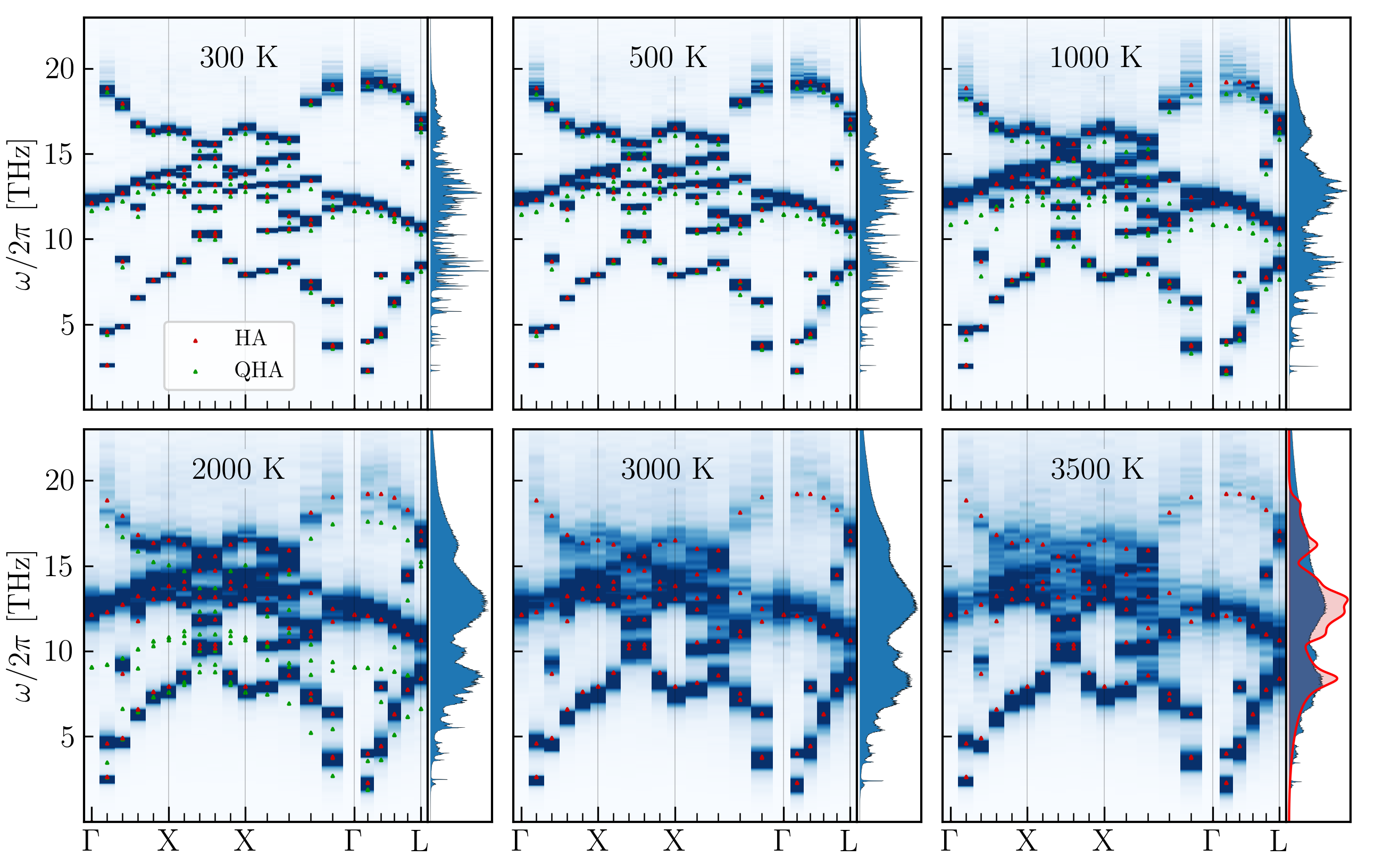
To disentangle the effects of thermal expansion from other mechanisms by which changes the spectra, let us turn our attention to Fig. 3, which presents the spectra calculated from MD simulations in which the volume of the crystal at all values of was constrained at the value . We will refer to the MD simulations whose spectra are presented in Figs. 1 and 3 as the and simulations, respectively.
The comparison between Figs. 1 and 3 demonstrates that the overall softening of most modes that occurs when the crystal is free to thermally expand does not occur when it is prevented from expanding. This, and the comparison with the QHA results below, confirm that thermal expansion bears most of the responsibilty for this softening.
The other features of the spectra that we have chosen to discuss, namely, that melting of the band structure begins with the LO mode near , before spreading to the BZ boundary and to other modes, are present in both Fig. 1 and Fig. 3. Therefore we can rule thermal expansion out as their cause. However it is worth noting that, at very high , the TO branches look much more like bands in the spectra than they do in the spectra. This may be because thermal expansion causes the TO and TA branches of the spectrum to overlap more in frequency, which would strengthen TO-TA interactions.
The QHA provides a reasonably accurate approximation to the phonon band structure up to at least , albeit one that is not noticeably closer to the MD band structure than the HA. However, its overestimation of the softening of TO frequencies is quite dramatic at and . Referring to Table 1, we see that the QHA lattice parameter is larger than the MD lattice parameter at each . However, these differences are much too small to explain the differences in frequency between the QHA bands and the MD bands. When the -dependent frequency of each mode is plotted as a function of the -dependent volume for both sets of calculations, the QHA curves lie below the MD curves and the gap between them widens as increases. Thermal expansion must explain the softening of the QHA bands with increasing , because the difference in is the only difference between calculations performed at different . However the degree to which the QHA oversoftens bands cannot be explained fully by inaccuracies of QHA thermal expansivities. We will return to this issue in Sec. V.4.
Karki et al. [2] found that QHA calculations of several thermodynamic properties started to deviate significantly from experimental measurements at around , with both thermal expansivity and the isobaric heat capacity being overestimated at high and the degrees to which they were overestimated increasing with . Therefore, to investigate whether or not this is a failure of the quasi-independent phonon assumption we have calculated the heat capacity within the QPA [3] For each mode we fitted the mode spectrum, , with a Lorentzian (Eq. 8), and treated the peak frequencies of the fitted Lorentzians as the QP frequencies.
The comparison between our QPA calculation, the QHA calculations of Karki et al., and the measurements of Isaak, Anderson, and Goto are presented in Fig. 4.
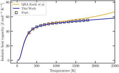
The QPA heat capacities are in excellent agreement with experiment at all values of for which experimental data is available. Therefore the inaccuracy of the QHA calculation at high is unlikely to be a result of treating phonons as quasi-independent excitations. It must be caused by the QHA failing to account for the self energies of these phonons. It is their self energies that turn them from NMVs into phonon QPs [3, 7].
V.4 Thermal broadening of bands
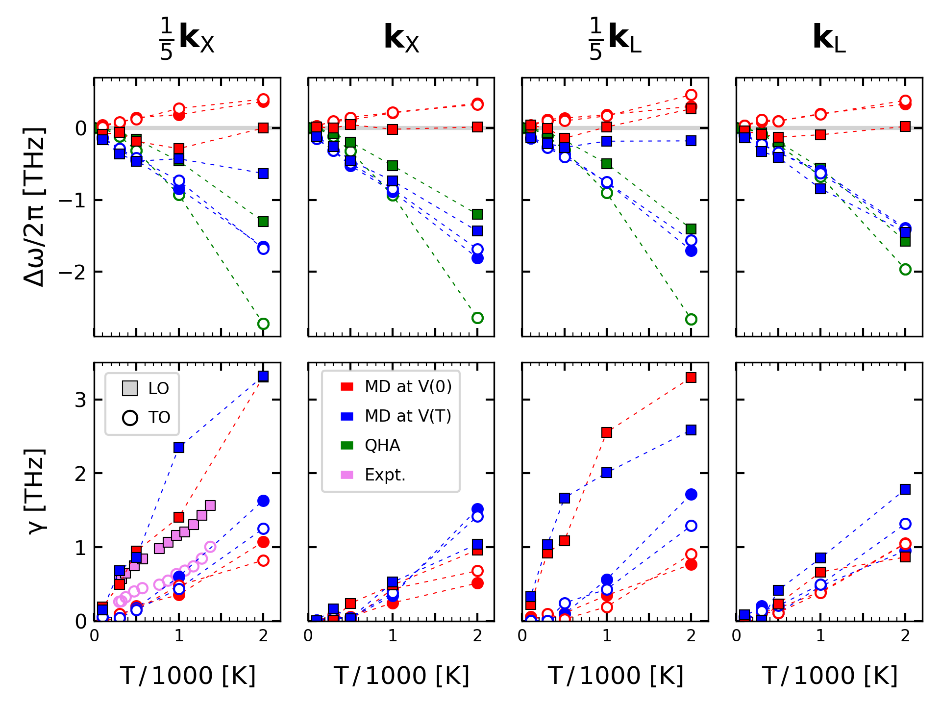
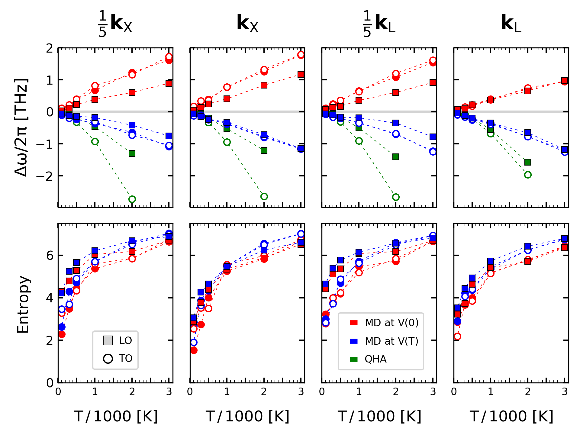
In Sec. V.2 we suggested some mechanisms by which LO bands can be broadened and shifted in frequency by acoustic modes, without acoustic bands degrading to the same degree. In Sec. V.3 we showed that thermal expansion causes most bands to shift to lower frequencies as increases, but is not the cause of the anomalous broadening of the LO band. In this section we take a closer look at thermal broadening of bands.
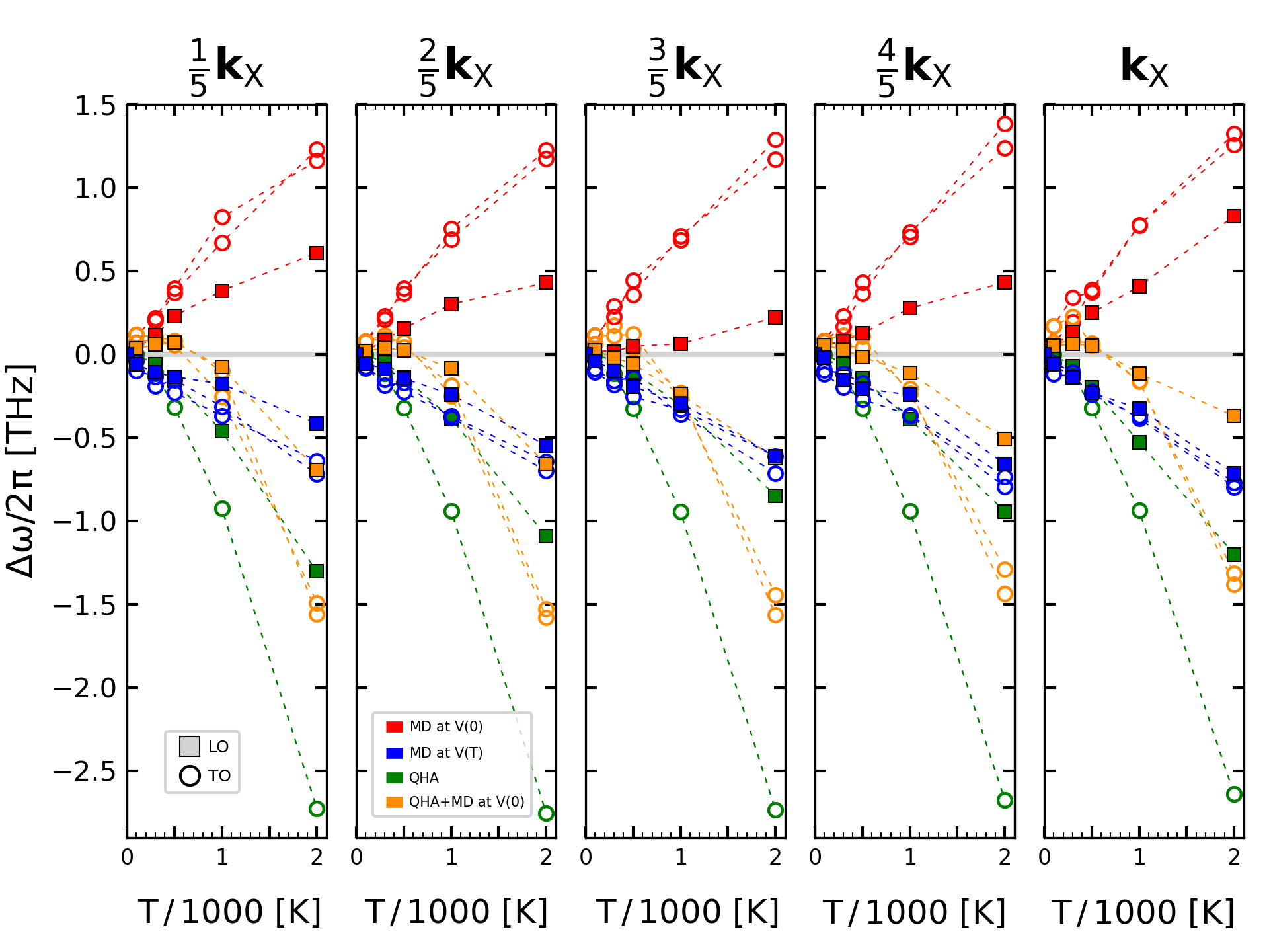
Fig. 5 presents the results of fitting Lorentzian functions (Eq. 8) to individual mode spectra (Eq. 3). The upper panels are plots of the -induced frequency shifts (Eq. 7), , of the three optical modes at each of the four wavevectors , , , and , where is the frequency of mode at zero pressure in the limit. In our MD simulations is the frequency of normal mode at the that minimizes the potential energy, whereas in the QHA it is its frequency at the that minimizes the sum of the potential energy and the zero-point energy of the phonon modes. Results from our and MD simulations are plotted in blue and red, respectively, and our QHA results are plotted in green. In each case the frequency shifts of TO and LO modes are plotted as circles and filled squares, respectively. We use the same symbols and colors to plot the Lorentzian linewidths in the lower panels, but instead of comparing to QHA linewidths, which we did not calculate, we compare to infrared reflectivity data of Calandrini et al. [12]. We find good agreement, despite comparing calculations at to measurements at much smaller wavevectors.
Overall, it is less easy to see firm trends in the data presented in Fig. 5 than it is to see them in Fig. 6, which uses the same symbols and colors to plot the shifts in the mean, , and the entropies, , of the mode distributions, . Therefore we include Fig. 5 for two reasons: to compare our MD linewidths with measured linewidths, and to illustrate why, for the purpose of investigating the effects of increasing , we have chosen to not assume that mode spectra are approximately Lorentzian. The entropy of a Lorentzian distribution is , so Fig. 5(b) might be clearer if its vertical axis had a logarithmic scale, but the entropy is a more general measure of uncertainty than either the width of the best-fit Lorentzian or its logarithm, and using it does not entail making any physical assumptions.
The QHA’s overestimation of the rates of decrease of optical mode frequencies with respect to is very clear in Fig. 6. Figure 7 demonstrates that the frequency shifts from our simulations are not well approximated by adding the shift caused by increasing at a fixed of to the shift caused by changing at a fixed of zero. The former is positive, which is consistent with the fact that phonon frequencies increase under pressure [2, 34]: As quantified in Sec. IV.2, when is fixed, increases as increases. Increasing makes it more difficult for individual primitive cells of the crystal to strain in order to accommodate optical mode displacements. This elastic response would reduce the energy cost of the optical displacements; therefore optical frequencies are increased when this response mechanism is suppressed. The orange symbols in Fig. 7 would coincide with their blue counterparts if changes to and contributed frequency shifts whose origins were approximately independent. The fact that they do not suggests that has other important effects. This highlights, again, the importance of interactions between phonons and the fact that each mode spectrum is not the spectrum of bare NMVs, but of QPs.
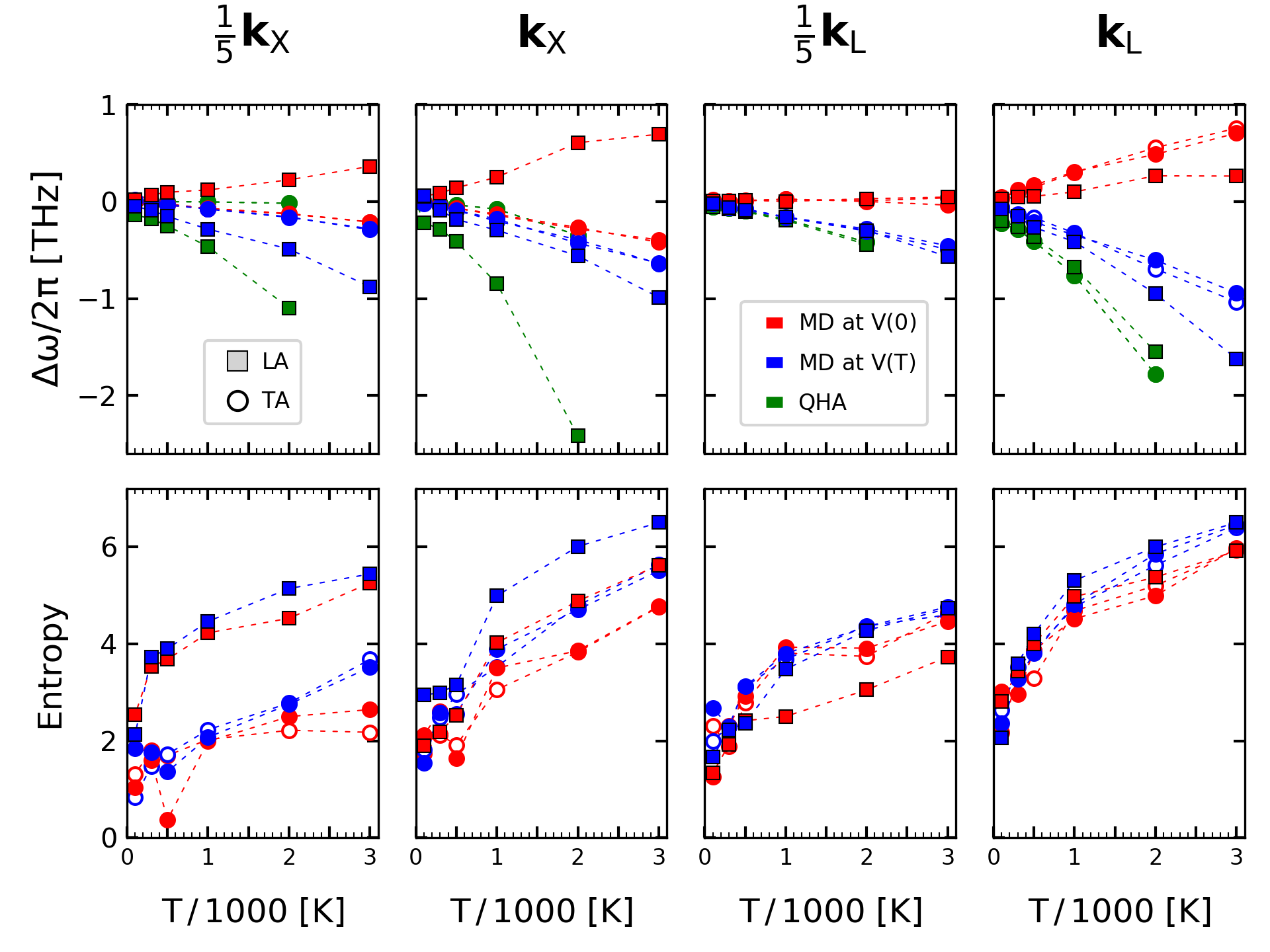
Figure 8 shows that TA modes are softened much less by than optical modes, especially at small wavevectors. At the QHA shifts are negligible and the and shifts are almost equal. At , by contrast, the shifts are negligible and the and QHA shifts are almost equal. At all wavevectors except , the QHA overestimates the softening of the LA mode at and . There is undoubtedly much to learn from a more detailed analysis of the acoustic modes than we have performed. The non-monotonicity of TA modes at low is particularly intriguing.
Notice that, at and , where acoustic frequencies are as large as optical frequencies, the entropies of acoustic and optical modes have similar magnitudes. However near the entropies of acoustic modes, and particularly the TA modes, are much smaller than those of optical modes. Near is where acoustic frequencies are small enough that adiabatic decoupling is likely to provide acoustic modes with the most protection from disorder generated by the optical modes.
Also notice that, at all values of , the LA mode’s entropy is significantly greater than the TA mode’s entropy at ; whereas at it is the TA mode whose entropy is larger at low ; and at the LA and TA modes have similar entropies. Entropy quantifies uncertainty, which increases with a mode distribution’s width. Therefore, Fig. 8 quantifies our observation in Sec. V.2.3 that, at low , there is broadening of the LA band along and of the TA bands along .
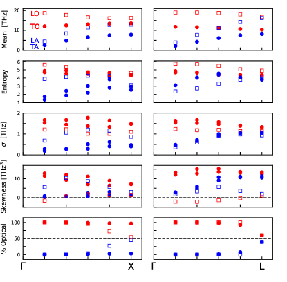
Figure 9 provides more insight into how the mode spectra change between the center and the boundary of the BZ. It consists of five vertically-stacked pairs of plots, with the horizontal axes of each pair’s left-hand and right-hand plots specifying one of the five finite wavevectors in our simulations along and , respectively. The data plotted in the lowermost pair of plots applies to the limit, because it was calculated from normal mode eigenvectors. We will discuss it below. The four uppermost pairs are plots of characteristics of the mode spectra from MD simulations at . The uppermost plots are simply plots of the mean frequencies; i.e., the bands. The next panels down are plots of the modes’ entropies, (Eq. 9). The third panels down are plots of the standard deviations () of the mode spectra, which we include only to allow to be compared to as a measure of thermal disorder. The plots second from the bottom show that most of the mode spectra are skewed towards higher frequencies, which would be consistent with them leaving behind a high-frequency tail when thermal expansions shifts their means downwards.
We will not speculate further about why most mode spectra have positive skewnesses. However in Sec. V.2.3 we suggested a mechanism that might contribute negatively to the skewness of only one of the six modes: An acoustic perturbation that warps is likely to reduce its magnitude, thereby lowering . Therefore a thermal distribution of acoustic perturbations might contribute low-frequency tails to LO mode spectra. This might explain why the LO mode has a skewness that is smaller in magnitude than other modes when it is positive, why it is the only mode whose skewness is negative at some wavevectors, and why the skewness changes from negative to positive between the BZ center and its boundary.
Now let us examine the plots of entropy in Fig. 9. Notice that, starting at or , the acoustic bands’ entropies increase, initially, as increases. This is to be expected because each mode’s entropy vanishes in the limit and it is only the interactions between modes that makes it finite. Acoustic modes’ frequencies move closer to those of optical modes as their wavevectors move away from the BZ center. Therefore, we should expect their interactions with optical modes to strengthen as increases, and this would increase their entropies.
If a mode was damped by many weak interactions, its entropy would increase gradually and monotonically as either the number of interactions or their strengths increased gradually. However, sudden reductions of entropy occur to the LA mode and the TA modes along ; and there is a less dramatic reduction of the TA modes’ entropies along . After increasing monotonically between and , the entropies of the LA band and the higher-entropy TA mode drop abruptly at . In the right-hand plot the entropies of both TA bands suddenly begin to decrease at .
These kinks in the entropy as a function of are interesting because they suggest the existence of strong interactions between modes, which contribute sizeable fractions of their total entropies. If a mode’s entropy only had contributions from weak interactions, a sudden decrease would require many interactions to weaken or vanish simultaneously (at the same wavevector). This is improbable. Each kink is much more likely to be explained by the disappearance or weakening of few very strong interactions, than by many weak ones. Therefore a kink in a band’s entropy is likely to mean that, on the higher-entropy side of the kink, the mode is involved in at least one particularly-strong interaction.
The fact that the entropy of the LA mode at is so high adds to the suspicion that it is caused by coupling to the LO mode, because is so low that only TA modes have similar frequencies. However, the TA modes’ entropies are smaller, suggesting that they do not interact with other modes as strongly as the LA mode does. Furthermore, if the high entropy of the LA band was caused by almost-resonant coupling between LA and TA modes, it should decrease with increasing , because and rapidly diverge. For a similar reason, the fact that the TO modes’ entropies remain relatively constant as approaches makes it unlikely that the LA entropy has a large contribution from LA-TO coupling. The LA-TO interaction should strengthen as their frequencies get closer, which would increase the TO entropy.
However, if the LA entropy was high due to LA-LO coupling, we would not necessarily see the LO mode entropy increase as increased. If the high LO entropy was caused by the LA mode warping , the effects of this disruption on the LO band would not necessarily increase as drew closer to , because the strength of this coupling mechanism does not rely on the coupled modes having similar frequencies. Furthermore, the degree to which shifts upwards decreases with increasing wavevector. Therefore, if the high LO entropy was caused by warping of , it should decrease with increasing , as it can be seen to do in Fig. 9. This diminishing importance of as the BZ boundary is approached would also contribute negatively to the LA band’s entropy, but the increase of the LA band’s frequency means that its interactions with most optical modes strengthen with increasing wavevector as it gets closer to resonance with them. This positive contribution to its entropy might more than offset the entropy reduction caused by its interaction with the LO mode weakening. A further clue that the high entropy of the LA mode is caused by its interaction with the LO mode via warping of is that vanishes at , which is where the LA entropy suddenly drops. The value it drops to is similar to that of the blue TA mode, which increases monotonically between and .
An obvious question to address is why the entropy of one of the TA bands increases more than the other, before also dropping suddenly at . The entropy of this band increases much more rapidly than the entropy of the other TA band, despite their mean frequencies remaining equal. However, it is important to note that the eigenvectors of two degenerate modes can be rotated in the two-dimensional space that they span, without changing their frequencies. For this reason, the two TA bands do not have independent identities and, for some rotations of TA eigenvectors within the subspace that they span, the entropies of the bands would be equal. Therefore we should not refer to entropies of the two TA bands individually; we should say that the combined entropy of the TA modes increases with increasing wavevector along , before suddenly decreasing at . This means that the results plotted in the left-hand panels of Fig. 9 are consistent with acoustic warping of , which mostly involves the LA band near , but with the TA modes becoming more involved as the BZ boundary is approached.
The sudden decrease of the TA entropy at is difficult to explain if its increase between and is caused by coupling to the TO modes. The data plotted in the bottom left panel of Fig. 9 also makes TO-TA coupling less likely to be responsible for the TA entropy being nonmonotonic. This is a plot of the degree to which each mode is an optical mode. An optical mode modulates the cation-anion displacement, whereas an acoustic mode modulates their center of mass. Therefore, instead of expressing eigenvectors in terms of displacements of Mg and O ions, we can express them in terms of Mg-O relative displacements and center of mass displacements. The former vanishes for an acoustic mode, the latter vanishes for an optical mode. Therefore, we use times the magnitude of latter divided by the magnitude of their sum to quantify the degree to which each mode is an optical mode. What we find is that, at , the LA and LO modes become significantly optical and acoustic, respectively. In other words, they mix strongly to become acoustic/optical hybrids.
At the polarization vectors of the LA and LO modes are identical, by symmetry. Mathematically, the difference in their frequencies can be viewed as a consequence of their normalized eigenvectors being different scalar multiples of the same polarization vector. The LO and LA eigenvectors are the polarization vector multiplied by the square roots of the O and Mg masses, respectively.
It is well known that when two modes couple strongly enough, they tend to hybridize: each one’s eigenvector becomes a mix of both eigenvectors, such that the modes described by the hybrid eigenvectors interact much more weakly. This is what causes avoided crossings in band structures. The LO-LA hybridization does not tell us anything directly about TO-TA coupling, but the bottom left plot of Fig. 9 shows that the TO and TA modes do not hybridize noticeably. At each TA (TO) mode is only optical (acoustic), and this increases to only at . Therefore the sudden decrease of the TA modes’ entropy at is unlikely to be a consequence of hybridization and we must look elsewhere for an explanation of it. The involvement of the TA modes in the acoustic-LO coupling is an obvious alternative explanation.
Now let us turn our attention to the path . The bottom-right plot of Fig. 9 shows that the TO and TA modes begin to hybridize at , and that all modes become hybrids of optical and acoustic modes at , with each mode’s optical/acoustic ratio being approximately or . Therefore the non-monotonic behaviour of the TA entropy might be explained by its sudden decoupling from the TO mode when they transform into TO/TA hybrids. This would make sense because they are both transverse modes, which become very close in frequency near . Therefore it seems plausible to interpret the kink in the entropy as a signature of strong TO-TA coupling at , which would explain why the entropy of the TA mode is greater than that of the LA mode near .
There are also some strong hints that acoustic modes are disrupting along . Firstly, the LO mode has the highest entropy, despite being the least active mode at low . Secondly, the LO mode has a negative skewness until vanishes at , which is consistent with the acoustic warping of giving it a low-frequency tail. Thirdly, the variation of the skewness with appears to mirror the variation of the mean frequency: As one increases the other decreases. This is consistent with the negative LO skewness being caused by this mechanism because it is the increasing strength of that causes to increase between and . As the field’s contribution to increases in magnitude, becomes more vulnerable to being lowered by acoustic perturbations.
All of the acoustic-LO coupling might be LA-LO coupling, but it is also possible that the TA mode is involved. However, near the BZ center, strong TA-LO coupling via TA disruption of requires the lateral extent of the LO phonon to be not much greater than its wavelength. This is because, if we approximately describe as a stack of parallel uniformly-charged infinite planes, a transverse displacement of each plane would not alter the constant field emanating from it. At finite the region perturbed by an LO phonon in a plane perpendicular to has a finite area. Therefore transverse displacements would change near the boundary of this region and, if a large enough fraction of the atoms participating in the LO motion were affected by this change, a TA phonon could couple significantly to it by this mechanism.
When the LO wavelength is small, on the other hand, the crystal planes displaced laterally by a TA phonon cannot be treated as uniformly charged; their atomistic structures have a significant influence on the value of . Therefore, near the BZ boundary there could be strong TA-LO coupling for LO phonons whose lateral extents are much larger than their wavelengths.
VI Conclusions
In this work we have studied strong phononic correlation in crystalline MgO with a method of calculating vibrational spectra that does not suffer from the limitations of perturbation theories or mean-field theories, and which can produce accurate wavevector-resolved spectra with enough detail to observe bandstructures. These calculations, and recent similar calculations by Lahnsteiner and Bokhdam [33], have been made possible by force fields whose parameters are fit to vast quantities of data calculated ab initio [87, 22, 26, 27, 32], and whose low computational expense, relative to ab initio MD, makes calculations of high resolution spectra possible.
As shown in Appendix A and Ref. 48, the method we have used to calculate spectra from our MD simulations is much more powerful and generally-applicable than existing derivations of it suggest [40, 41, 42, 43, 9, 24, 44, 45, 46, 47]. It is not a new method, having been used to calculate frequency- and wavevector-resolved spectra at least as far back as 2006 [8], and to calculate spectra as functions of frequency only for many years prior to that. However existing derivations of it do not justify using it to calculate spectra at very high , when phononic correlation is strong, as we have done. Therefore it has usually been interpreted as a method of calculating the VDOS at thermal equilibrium when phonons do not interact (i.e., in the limit) or when their interactions are sufficiently simple that each phonon is an exponentially-decaying harmonic wave, in which case its spectral peak is Lorentzian [88, 43, 24, 33].
However, we have shown that it is an exact method, whose applicability is not restricted to crystals, to low , or even to states of thermal equilibrium. This means that it is a powerful tool for studying vibrations in materials, which complements and is complemented by, perturbation theories. It can also be used to assess the accuracies of perturbative methods, mean-field methods, and other methods that rely on simplifying assumptions, such as the assumption of a state of thermal equilbrium [20]. For these reasons, it seems likely to play an increasingly important role as it becomes possible to calculate forces accurately and efficiently for more materials.
For example, it should help with the development of materials that are either transparent or opaque to THz radiation in a particular frequency window. In other words, it should help to guide us in the rational design of materials that behave as THz bandpass filters for use as active or passive components of THz devices.
Another application is in the study of order-disorder transitions between crystalline phases, which occur when a single phonon band melts but the other bands do not, causing displacements and velocities along the eigenvectors of the melted band’s modes to become disordered. This critical weakening of correlations causes both the time average and the spatial average of the displacements to vanish. As a result, when the crystal is observed at either a low spatial resolution or a low temporal resolution, its symmetry appears to have increased. The ability to see how the vibrational spectrum changes as crosses the transition temperature may lead to step changes in our understandings of these transitions, or even to a step change in our understanding of this class of transitions.
A third application is in the study of materials at very high , such as thermal barrier coatings, where there are high densities of defects, and therefore high densities of vibrations that are localized in spacetime and delocalized in reciprocal spacetime. A fourth application, which is related to the third, is in the identification or design of materials with reduced or enhanced thermal conductivities. For example, the thermal conductivities of materials with low-frequency localized rattler modes [89] are low because the energy of these modes, being localized in spacetime, is delocalized in -space. Therefore they overlap with acoustic modes in reciprocal spacetime, which allows the acoustic modes to couple with them, and with one another through them, to disperse their energy.
However the generality of this method means that one of the most important applications of it may be to study general properties of strong phononic correlation. The simplest and most obvious first step is to study the strengthening of phononic correlation in a simple prototype crystal as it is heated. This has been the purpose of this work.
We have found that, despite the apparent banality of crystalline MgO at thermal equilibrium, there is so much to be learned from the spectra presented herein that we have been forced to focus most of our analyses of them on a few of their gross features. We provide our raw spectra, in the form of tabulations of at each value of , as supplementary material in case others wish to analyse it further or differently [77].
By calculating spectra at both constant volume and constant pressure, we have been able to show conclusively that some features of the spectrum’s dependence, such as the tendency of bands to soften as increases, are consequences of thermal expansion; and that others, such as the rapid degradation of the LO band, are not. We have shed substantial light on the strengths and limitations of the quasiharmonic approximation and we have shown that some of its weaknesses are rectified by the quasiparticle approximation.
Most importantly, we have identified, and discussed in some detail, two physical considerations that are likely to have observable consequences for many or most crystals. The first is that LO phonons are highly sensitive to the amplitudes of acoustic phonons because a large fraction ( for MgO) of is contributed by the LO mode’s intrinsic field, which acoustic phonons warp. This simple mechanism must occur, to some degree, in every partially-ionic crystal, because every LO phonon has an intrinsic field that opposes its motion and increases its frequency. The second consideration is that, despite this strong acoustic-LO coupling, long wavelength acoustic phonons are adiabatically decoupled from LO modes: they strongly modulate the energies and frequencies of LO modes, while maintaining approximately-constant energies and frequencies themselves.
The feature of the spectrum’s -dependence that led us to these ideas and explanations is very similar to features that have been observed experimentally in the spectra of other ionic crystals since the 1960s [58, 59, 60, 61, 62, 63, 64, 65, 66, 67]. It has also been studied in MgO and similar materials using perturbation theory [38, 12, 39], but it has lacked a simple and intuitive physical explanation until now.
Acknowledgments
GC was supported through a studentship in the Centre for Doctoral Training on Theory and Simulation of Materials at Imperial College London funded by the EPSRC (EP/L015579/1).
Appendix A Distribution of the kinetic energy of a vibrating string in reciprocal spacetime
Consider a taut string, of uniform mass per unit length , whose ends are fixed at and , and which lies along the axis when it is at equilibrium. Its displacement from equilibrium at spacetime coordinates is denoted by , and its kinetic energy per unit length is , where and is an infinitesimal length.
Let us assume that the string only moves during the time interval , or that it is only observed for times . In the latter case, we assume that, at each , has been tapered smoothly, but arbitrarily rapidly, to zero at times and . Similarly, is both smooth and vanishes for . Therefore, for all of our purposes within this appendix, is equivalent to and is equivalent to .
The average, over interval , of the string’s kinetic energy per unit length at is
| (10) | ||||
| (11) |
where is the unitary Fourier transform of with respect to time, and we have used Parseval’s theorem [50] to reach Eq. 11 from Eq. 10. Since is real, , which implies that . Therefore, . If we integrate over all and use Parseval’s theorem again we find that the average kinetic energy of the entire string is
where is the unitary FT of with respect to both and , i.e.,
Therefore, the string’s average kinetic energy divided by its length is
| (12) |
The VVCF is defined as
If we express and in terms of , perform the integrals over and before the integrals over frequencies and wavevectors, and use the identities and , this becomes
Therefore the FT of with respect to both and is , and Eq. 12 becomes
| (13) |
Now let us assume that string’s velocity is sampled at evenly-spaced times between and and at evenly-space points between and . Then the VVCF becomes
where the sums are over the sampled times and positions.
Now, because vanishes when , the smallest observable wavevector and the smallest observable difference between two wavevectors are both equal to . Similarly, because vanishes when , the smallest observable frequency and the smallest observable difference between two frequencies are both equal to . This implies that there are only observable frequencies and observable wavevectors, and the integrals in Eq. 13 must be approximated as sums over these observable values. If we define , we can express the discretized version of Eq. 13 as
and the discrete FT of as
Therefore the average kinetic energy of the string per unit of its length is a sum over all sampled frequencies and wavevectors of the discrete FT of the VVCF. The linearity of the FT implies that each term in this sum is the contribution to the average kinetic energy of motions with wavevector and frequency .
Appendix B The force field
We use a classical dipole-polarizable potential of the form described in Refs. [25], [28], and [68]. It includes a sum of purely-pairwise interaction energies of the form
where is the distance between ions and , and and are their charges. The parameters , and define the Morse potential and, along with the charges, are among the parameters that are fit to reproduce forces, stress tensors, and energy differences calculated ab initio with density functional theory. A list of all potential parameters and their values are provide in Table 2.
In addition to the pairwise part of the potential, the oxygen anion is assigned a polarizability, , which is used to assign a dipole moment to each anion as follows:
where the second term on the right hand side is the dipole moment induced on ion by the local electric field from the charges and dipole moments of all other ions, and
| where | ||||
is a short range contribution to the dipole from an anion’s electron cloud changing shape as its neighbouring ions move. Since each dipole moment depends on the values of all others, the set of all dipole moments is calculated, at each set of ionic positions, by iterating them to self-consistency [25]. After self consistency has been achieved charge-dipole and interaction energies are added to for each pair of ions that includes an oxygen ion and dipole-dipole interaction energies are added to it when and are both oxygen ions.
| Mg | O | Mg-Mg | Mg-O | O-O | |
|---|---|---|---|---|---|
| charges | |||||
| q | 1.415382 | -1.415382 | |||
| 0 | 3.0945 10-3 | 2.161 10-3 | |||
| 25.1073 | 10.1621 | 8.9925 | |||
| 26.9788 | 4.9640 | 6.1491 | |||
| dipoles | |||||
| 0 | 9.6565 | ||||
| 0 | 1.8713 | 0 | |||
| 0 | -1.6809 | 0 |
References
- Sangster et al. [1970] M. J. L. Sangster, G. Peckham, and D. H. Saunderson, Lattice dynamics of magnesium oxide, J. Phys. C: Solid State Phys. 3, 1026 (1970).
- Karki et al. [2000] B. B. Karki, R. M. Wentzcovitch, S. de Gironcoli, and S. Baroni, High-pressure lattice dynamics and thermoelasticity of MgO, Phys. Rev. B 61, 8793 (2000).
- D. C. Wallace [1972] D. C. Wallace, Thermodynamics of Crystals (Dover Publications Inc., New York, 1972).
- Jones and March [1973] W. Jones and N. H. March, Theoretical solid state physics: Volume I (Dover Publications Inc., New York, 1973).
- Ashcroft and Mermin [1976] N. W. Ashcroft and N. D. Mermin, Solid State Physics, HRW international editions (Holt, Rinehart and Winston, 1976).
- Cohen and Louie [2016] M. L. Cohen and S. G. Louie, Fundamentals of Condensed Matter Physics (Cambridge University Press, 2016).
- Mattuck [1976] R. D. Mattuck, A Guide to Feynman Diagrams in the Many-body Problem, Advanced Book Program - McGraw-Hill Book Company (McGraw-Hill, 1976).
- Tangney et al. [2006] P. Tangney, M. L. Cohen, and S. G. Louie, Giant wave-drag enhancement of friction in sliding carbon nanotubes, Phys. Rev. Lett. 97, 195901 (2006).
- Zhang et al. [2014] D.-B. Zhang, T. Sun, and R. M. Wentzcovitch, Phonon quasiparticles and anharmonic free energy in complex systems, Phys. Rev. Lett. 112, 058501 (2014).
- Breeze [2016] J. Breeze, Temperature and Frequency Dependence of Complex Permittivity in Metal Oxide Dielectrics: Theory, Modelling and Measurement (Springer International Publishing, 2016).
- Lu et al. [2018] Y. Lu, T. Sun, and D.-B. Zhang, Lattice anharmonicity, phonon dispersion, and thermal conductivity of PbTe studied by the phonon quasiparticle approach, Phys. Rev. B 97, 174304 (2018).
- Calandrini et al. [2021] E. Calandrini, L. Paulatto, D. Antonangeli, F. He, R. P. S. M. Lobo, F. Capitani, J.-B. Brubach, P. Roy, L. Vincent, and P. Giura, Limits of the quasiharmonic approximation in MgO: Volume dependence of optical modes investigated by infrared reflectivity and ab initio calculations, Phys. Rev. B 103, 054302 (2021).
- Sirtori [2002] C. Sirtori, Bridge for the terahertz gap, Nature 417, 132 (2002).
- Perkowitz [2020] S. Perkowitz, Navigating the terahertz gap, Physics World 33, 37 (2020).
- Hooton [1955] D. J. Hooton, A new treatment of anharmonicity in lattice thermodynamics: I, Lond. Edinb. Dublin philos. mag. j. sci. 46, 422 (1955).
- Werthamer [1970] N. R. Werthamer, Self-consistent phonon formulation of anharmonic lattice dynamics, Phys. Rev. B 1, 572 (1970).
- Hellman et al. [2013] O. Hellman, P. Steneteg, I. A. Abrikosov, and S. I. Simak, Temperature dependent effective potential method for accurate free energy calculations of solids, Phys. Rev. B 87, 104111 (2013).
- Tadano and Tsuneyuki [2015] T. Tadano and S. Tsuneyuki, Self-consistent phonon calculations of lattice dynamical properties in cubic with first-principles anharmonic force constants, Phys. Rev. B 92, 054301 (2015).
- Bianco et al. [2017] R. Bianco, I. Errea, L. Paulatto, M. Calandra, and F. Mauri, Second-order structural phase transitions, free energy curvature, and temperature-dependent anharmonic phonons in the self-consistent harmonic approximation: Theory and stochastic implementation, Phys. Rev. B 96, 014111 (2017).
- Monacelli et al. [2021] L. Monacelli, R. Bianco, M. Cherubini, M. Calandra, I. Errea, and F. Mauri, The stochastic self-consistent harmonic approximation: calculating vibrational properties of materials with full quantum and anharmonic effects, J. Phys. Condens. Matter 33, 363001 (2021).
- Zacharias et al. [2023] M. Zacharias, G. Volonakis, F. Giustino, and J. Even, Anharmonic lattice dynamics via the special displacement method, Phys. Rev. B 108, 035155 (2023).
- Tangney and Scandolo [2003] P. Tangney and S. Scandolo, A many-body interatomic potential for ionic systems: Application to MgO, J. Chem. Phys. 119, 9673 (2003), https://doi.org/10.1063/1.1609980 .
- Tangney and Scandolo [2009] P. Tangney and S. Scandolo, Melting slope of MgO from molecular dynamics and density functional theory, J. Chem. Phys. 131, 124510 (2009), https://doi.org/10.1063/1.3238548 .
- Sun et al. [2014] T. Sun, D.-B. Zhang, and R. M. Wentzcovitch, Dynamic stabilization of cubic perovskite at high temperatures and pressures from ab initio molecular dynamics, Phys. Rev. B 89, 094109 (2014).
- Tangney and Scandolo [2002] P. Tangney and S. Scandolo, An ab initio parametrized interatomic force field for silica, J. Chem. Phys. 117, 8898 (2002).
- Behler and Parrinello [2007] J. Behler and M. Parrinello, Generalized neural-network representation of high-dimensional potential-energy surfaces, Phys. Rev. Lett. 98, 146401 (2007).
- Bartók et al. [2010] A. P. Bartók, M. C. Payne, R. Kondor, and G. Csányi, Gaussian approximation potentials: The accuracy of quantum mechanics, without the electrons, Phys. Rev. Lett. 104, 136403 (2010).
- Han et al. [2010] X. J. Han, L. Bergqvist, P. H. Dederichs, H. Müller-Krumbhaar, J. K. Christie, S. Scandolo, and P. Tangney, Polarizable interatomic force field for TiO2 parametrized using density functional theory, Phys. Rev. B 81, 134108 (2010).
- Sarsam et al. [2013a] J. Sarsam, M. W. Finnis, and P. Tangney, Atomistic force field for alumina fit to density functional theory, The Journal of Chemical Physics 139, 10.1063/1.4832695 (2013a), 204704, .
- Szlachta et al. [2014] W. J. Szlachta, A. P. Bartók, and G. Csányi, Accuracy and transferability of gaussian approximation potential models for tungsten, Phys. Rev. B 90, 104108 (2014).
- Deringer and Csányi [2017] V. L. Deringer and G. Csányi, Machine learning based interatomic potential for amorphous carbon, Phys. Rev. B 95, 094203 (2017).
- Unke et al. [2021] O. T. Unke, S. Chmiela, H. E. Sauceda, M. Gastegger, I. Poltavsky, K. T. Schütt, A. Tkatchenko, and K.-R. Müller, Machine learning force fields, Chemical Reviews 121, 10142 (2021).
- Lahnsteiner and Bokdam [2022] J. Lahnsteiner and M. Bokdam, Anharmonic lattice dynamics in large thermodynamic ensembles with machine-learning force fields: , a phonon liquid with Cs rattlers, Phys. Rev. B 105, 024302 (2022).
- Ghose et al. [2006] S. Ghose, M. Krisch, A. R. Oganov, A. Beraud, A. Bosak, R. Gulve, R. Seelaboyina, H. Yang, and S. K. Saxena, Lattice dynamics of MgO at high pressure: Theory and experiment, Phys. Rev. Lett. 96, 035507 (2006).
- Dekura et al. [2013] H. Dekura, T. Tsuchiya, and J. Tsuchiya, Ab initio lattice thermal conductivity of perovskite as found in earth’s lower mantle, Phys. Rev. Lett. 110, 025904 (2013).
- Kimura et al. [2017] T. Kimura, H. Ohfuji, M. Nishi, and T. Irifune, Melting temperatures of MgO under high pressure by micro-texture analysis, Nat. Comm. 8, 15735 (2017).
- Fugallo et al. [2018] G. Fugallo, B. Rousseau, and M. Lazzeri, Infrared reflectance, transmittance, and emittance spectra of MgO from first principles, Phys. Rev. B 98, 184307 (2018).
- Giura et al. [2019] P. Giura, L. Paulatto, F. He, R. P. S. M. Lobo, A. Bosak, E. Calandrini, L. Paolasini, and D. Antonangeli, Multiphonon anharmonicity of MgO, Phys. Rev. B 99, 220304 (2019).
- Togo et al. [2022] A. Togo, H. Hayashi, T. Tadano, S. Tsutsui, and I. Tanaka, LO-mode phonon of KCl and NaCl at K by inelastic X-ray scattering measurements and first principles calculations, J. Phys. Condens. Matter 34, 365401 (2022).
- Dove [1993] M. T. Dove, Introduction to Lattice Dynamics, Cambridge Topics in Mineral Physics and Chemistry (Cambridge University Press, 1993).
- Lee et al. [1993] C. Lee, D. Vanderbilt, K. Laasonen, R. Car, and M. Parrinello, Ab initio studies on the structural and dynamical properties of ice, Phys. Rev. B 47, 4863 (1993).
- Ladd et al. [1986] A. J. C. Ladd, B. Moran, and W. G. Hoover, Lattice thermal conductivity: A comparison of molecular dynamics and anharmonic lattice dynamics, Phys. Rev. B 34, 5058 (1986).
- Sun et al. [2010] T. Sun, X. Shen, and P. B. Allen, Phonon quasiparticles and anharmonic perturbation theory tested by molecular dynamics on a model system, Phys. Rev. B 82, 224304 (2010).
- Meyer and Comtesse [2011] R. Meyer and D. Comtesse, Vibrational density of states of silicon nanoparticles, Phys. Rev. B 83, 014301 (2011).
- Thomas et al. [2013] M. Thomas, M. Brehm, R. Fligg, P. Vöhringer, and B. Kirchner, Computing vibrational spectra from ab initio molecular dynamics, Phys. Chem. Chem. Phys. 15, 6608 (2013).
- Tuckerman [2010] M. Tuckerman, Statistical Mechanics: Theory and Molecular Simulation, Oxford Graduate Texts (OUP Oxford, 2010).
- Cupo et al. [2019] A. Cupo, D. Tristant, K. Rego, and V. Meunier, Theoretical analysis of spectral lineshapes from molecular dynamics, npj Comp. Mat. 5, 82 (2019).
- Tangney [2023] P. Tangney, Wave theory of lattice dynamics (2023), manuscript in preparation.
- Cowley [1963] R. A. Cowley, The lattice dynamics of an anharmonic crystal, Advances in Physics 12, 421 (1963).
- Strichartz [2003] R. S. Strichartz, A Guide To Distribution Theory And Fourier Transforms (Scientific, World, 2003).
- Aulbur et al. [2000] W. G. Aulbur, L. Jönsson, and J. W. Wilkins, Quasiparticle calculations in solids, in Solid State Physics, Solid State Physics, Vol. 54, edited by H. Ehrenreich and F. Spaepen (Academic Press, 2000) pp. 1–218.
- Cochran [1960] W. Cochran, Crystal stability and the theory of ferroelectricity, Advances in Physics 9, 387 (1960).
- Stern [2004] E. A. Stern, Character of order-disorder and displacive components in barium titanate, Phys. Rev. Lett. 93, 037601 (2004).
- Hlinka et al. [2008] J. Hlinka, T. Ostapchuk, D. Nuzhnyy, J. Petzelt, P. Kuzel, C. Kadlec, P. Vanek, I. Ponomareva, and L. Bellaiche, Coexistence of the phonon and relaxation soft modes in the terahertz dielectric response of tetragonal , Phys. Rev. Lett. 101, 167402 (2008).
- Gu et al. [2021] F. Gu, E. Murray, and P. Tangney, Carrier-mediated control over the soft mode and ferroelectricity in , Phys. Rev. Mater. 5, 034414 (2021).
- Riley et al. [2002] K. F. Riley, M. P. Hobson, and S. J. Bence, Probability, in Mathematical Methods for Physics and Engineering: A Comprehensive Guide (Cambridge University Press, 2002) p. 961–1063, 2nd ed.
- Shannon [1948] C. E. Shannon, A mathematical theory of communication, The Bell System Technical Journal 27, 379 (1948).
- Woods et al. [1960] A. D. B. Woods, W. Cochran, and B. N. Brockhouse, Lattice dynamics of alkali halide crystals, Phys. Rev. 119, 980 (1960).
- Woods et al. [1963] A. D. B. Woods, B. N. Brockhouse, R. A. Cowley, and W. Cochran, Lattice dynamics of alkali halide crystals. II. experimental studies of KBr and NaI, Phys. Rev. 131, 1025 (1963).
- Raunio et al. [1969] G. Raunio, L. Almqvist, and R. Stedman, Phonon dispersion relations in NaCl, Phys. Rev. 178, 1496 (1969).
- Raunio [1969] G. Raunio, Phonon widths in NaCl, KCl, and RbCl from neutron measurements, physica status solidi (b) 35, 299 (1969), .
- Lowndes [1970] R. P. Lowndes, Influence of lattice anharmonicity on the longitudinal optic modes of cubic ionic solids, Phys. Rev. B 1, 2754 (1970).
- Chang and Mitra [1972] I. F. Chang and S. S. Mitra, Temperature dependence of long-wavelength optic phonons of NaF single crystals, Phys. Rev. B 5, 4094 (1972).
- Nilsson [1981] G. G. Nilsson, Phonon widths in RbBr at , , and K from neutron measurements, physica status solidi (b) 106, 271 (1981).
- Cowley et al. [1983] E. R. Cowley, S. Satija, and R. Youngblood, Line shapes of longitudinal-optic phonons in sodium chloride at and K, Phys. Rev. B 28, 993 (1983).
- Shen et al. [2020] Y. Shen, C. N. Saunders, C. M. Bernal, D. L. Abernathy, M. E. Manley, and B. Fultz, Anharmonic origin of the giant thermal expansion of NaBr, Phys. Rev. Lett. 125, 085504 (2020).
- Shen et al. [2021] Y. Shen, C. N. Saunders, C. M. Bernal, D. L. Abernathy, T. J. Williams, M. E. Manley, and B. Fultz, Prediction and observation of intermodulation sidebands from anharmonic phonons in NaBr, Phys. Rev. B 103, 134302 (2021).
- Sarsam et al. [2013b] J. Sarsam, M. W. Finnis, and P. Tangney, Atomistic force field for alumina fit to density functional theory, J. Chem. Phys. 139, 204704 (2013b), https://doi.org/10.1063/1.4832695 .
- Mueller et al. [2020] T. Mueller, A. Hernandez, and C. Wang, Machine learning for interatomic potential models, J. Chem. Phys. 152, 050902 (2020).
- Perdew et al. [2008] J. P. Perdew, A. Ruzsinszky, G. I. Csonka, O. A. Vydrov, G. E. Scuseria, L. A. Constantin, X. Zhou, and K. Burke, Restoring the density-gradient expansion for exchange in solids and surfaces, Phys. Rev. Lett. 100, 136406 (2008).
- Madden and Wilson [1996] P. A. Madden and M. Wilson, Covalent effects in ‘ionic’ systems, Chem. Soc. Rev. 25, 339 (1996).
- Madden and Wilson [2000] P. A. Madden and M. Wilson, `covalent' effects in `ionic' liquids, J. Phys. Condens. Matter 12, A95 (2000).
- Wilson and Madden [1993] M. Wilson and P. A. Madden, Polarization effects in ionic systems from first principles, J. Phys. Condens. Matter 5, 2687 (1993).
- Fei [1999] Y. Fei, Effects of temperature and composition on the bulk modulus of (Mg,Fe)O, Am. Mineral. 84, 272 (1999).
- Liang et al. [2006] Y. Liang, C. R. Miranda, and S. Scandolo, Infrared and raman spectra of silica polymorphs from an ab initio parametrized polarizable force field, J. Chem. Phys. 125, 194524 (2006), https://doi.org/10.1063/1.2390709 .
- Belonoshko and Dubrovinsky [1996] A. B. Belonoshko and L. S. Dubrovinsky, Molecular dynamics of NaCl (B1 and B2) and MgO (B1) melting: Two-phase simulation, Am. Mineral. 81, 303 (1996), https://pubs.geoscienceworld.org/msa/ammin/article-pdf/81/3-4/303/4222305/am81_303.pdf .
- [77] See Supplemental Material at [URL will be inserted by publisher] for tabulations of the fourier-transformed mass-weighted velocity-velocity correlation functions, , at a range of temperatures before smoothing has been applied to them.
- Landau et al. [1976] L. Landau, E. Lifshitz, J. Sykes, and J. Bell, Mechanics: Volume 1, Course of theoretical physics (Elsevier Science, 1976).
- Arnold [1989] V. I. Arnold, Mathematical Methods of Classical Mechanics, 2nd ed., Graduate Texts in Mathematics (Springer New York, 1989).
- Spohn and Teufel [2001] H. Spohn and S. Teufel, Adiabatic decoupling and time-dependent Born–Oppenheimer theory, Commun. Math. Phys. 224, 113 (2001).
- Tangney [2006] P. Tangney, On the theory underlying the Car-Parrinello method and the role of the fictitious mass parameter, J. Chem. Phys. 124, 044111 (2006), https://doi.org/10.1063/1.2162893 .
- Gilz et al. [2016] L. Gilz, E. Thesing, and J. R. Anglin, Hamiltonian analogs of combustion engines: A systematic exception to adiabatic decoupling, Phys. Rev. E 94, 042127 (2016).
- Born and Huang [1988] M. Born and K. Huang, Dynamical Theory of Crystal Lattices, International series of monographs on physics (Clarendon Press, Oxford, UK, 1988).
- Resta and Vanderbilt [2007] R. Resta and D. Vanderbilt, Theory of polarization: A modern approach, in Physics of Ferroelectrics, Topics in Applied Physics, Vol. 105 (Springer Berlin, Heidelberg, 2007) pp. 31–68.
- Zhang and Zeng [2013] J. Zhang and Z. Zeng, Electronic and optical properties of perfect MgO and MgO with F center under high pressure, Int. J. Mod. Phys. C 24, 1350052 (2013).
- Isaak et al. [1989] D. G. Isaak, O. L. Anderson, and T. Goto, Measured elastic moduli of single-crystal MgO up to K, Phys. Chem. Miner. 16, 704 (1989).
- Ercolessi and Adams [1994] F. Ercolessi and J. B. Adams, Interatomic potentials from first-principles calculations: The force-matching method, Europhys. Lett. 26, 583 (1994).
- de Koker [2009] N. de Koker, Thermal conductivity of MgO periclase from equilibrium first principles molecular dynamics, Phys. Rev. Lett. 103, 125902 (2009).
- Christensen et al. [2008] M. Christensen, A. B. Abrahamsen, N. B. Christensen, F. Juranyi, N. H. Andersen, K. Lefmann, J. Andreasson, C. R. H. Bahl, and B. B. Iversen, Avoided crossing of rattler modes in thermoelectric materials, Nat. Mater. 7, 811 (2008).