Confidence intervals for performance estimates in 3D medical image segmentation

Abstract

Medical segmentation models are evaluated empirically. As such an evaluation is based on a limited set of example images, it is unavoidably noisy. Beyond a mean performance measure, reporting confidence intervals is thus crucial. However, this is rarely done in medical image segmentation. The width of the confidence interval depends on the test set size and on the spread of the performance measure (its standard-deviation across of the test set). For classification, many test images are needed to avoid wide confidence intervals. Segmentation, however, has not been studied, and it differs by the amount of information brought by a given test image. In this paper, we study the typical confidence intervals in medical image segmentation. We carry experiments on 3D image segmentation using the standard nnU-net framework, two datasets from the Medical Decathlon challenge and two performance measures: the Dice accuracy and the Hausdorff distance. We show that the parametric confidence intervals are reasonable approximations of the bootstrap estimates for varying test set sizes and spread of the performance metric. Importantly, we show that the test size needed to achieve a given precision is often much lower than for classification tasks. Typically, a 1% wide confidence interval requires about 100-200 test samples when the spread is low (standard-deviation around 3%). More difficult segmentation tasks may lead to higher spreads and require over 1000 samples.

I Introduction

Solid evaluation is crucial for automatic tools used to process medical images, as medical professionals must trust the automated system’s output. Most modern segmentation tools rely on deep learning [1], and their performance depends on details of the training run. Trained models are evaluated by using unseen data to estimate their expected performance. Evaluation is harder than it seems. First, it requires an adequate choice of metric [2, 3, 4]. Second, it is inevitably noisy, if only because it uses a finite number of samples. It is thus crucial to quantify the uncertainty on an estimated performance, for instance using confidence intervals (CIs). Indeed, model developers can easily fall into the trap of apparent model improvements due to evaluation noise, that do not generalize to new data, as in some medical-imaging competitions [5, 6].

And yet, evaluation uncertainty or CIs are seldom reported in the medical image segmentation literature (including in our own previous papers, e.g. [7, 8, 9]). To illustrate how prevalent the problem is, we conducted a survey of all papers on 3D medical image segmentation published in 2022 in the following three journals: IEEE Transactions on Medical Imaging, Medical Image Analysis and Journal of Medical Imaging. As reported in Table I, only 11 of the corresponding 133 paper reported CIs. Such quick survey, in no way exhaustive, does suggest that, across three representative journals of the community, the vast majority ($>90\%$) of recent papers do not report confidence intervals for their trained models.

Two main factors affect the precision of model evaluation: the size of the test set, and how much the performance metric varies across test-set samples. Given a high spread of the metric across the test set, the precision will be low and the confidence interval will be wider. Alternatively, increasing the sample size of the test set leads to tighter confidence intervals. In 3D medical image segmentation, the size of the set used to evaluate the performance is often of small to moderate size, typically in the order of dozens of subjects, at best hundreds, as obtaining the ground truth requires voxel-wise annotation by trained raters. One fear is thus that most segmentation performances assessments will be associated to large error bars. For image classification, studies have shown that large sample sizes are needed for a precise estimation of the prediction accuracy (typically 10,000 samples to achieve a $1\%$-wide confidence interval) [10, 11]. Surprisingly, this question has not yet been addressed for medical image segmentation.

This paper addresses the following questions. What precision can be expected in 3D medical image segmentation for typical test set sizes? How trustworthy are the average performance estimates (for instance Dice coefficients or Hausdorff distance) reported in medical image segmentation papers? The main objectives are: i) to raise awareness on the importance of reporting confidence interval on independent test sets; ii) to provide the community with typical values of CI that can be expected for various sample sizes and performance variability.

To this end, we present in this paper a series of experiments that deploy nnU-net [12] –a standard framework for medical image segmentation– on two classical segmentation tasks from the Segmentation Decathlon Challenge [13] in order to estimate confidence intervals that are obtained for test sets of variable size. For each task, we study the following performance measures: the Dice accuracy and the Hausdorff distance. We then report CIs using both bootstrap (which is the most general approach) and a parametric estimation, and varying the test set size. We find that the parametric estimation is in general reasonable, even for small test sets and for metrics which distribution is far from being Gaussian. Building on this, we perform simulations for other sizes and spreads. We demonstrate that the test size needed to achieve a given precision is lower for segmentation than for classification. This is due to the continuous nature of the evaluation metrics [14]. Indeed, segmentation algorithms are evaluated with continuous metrics that aggregate multiple observations at the level of a single image. As each image brings more information to characterize the errors of the algorithm, tight confidence intervals can often be obtained with a moderate number of images.

The remaining sections of this paper are organized as follows. In section II, we describe the statistical tools that we use in this paper to conduct our analysis. In section III, we present the datasets examined and the experimental setup. Section IV reports results on the whole test sets. In Section  V, we then experimentally study how the precision varies when varying the test set size. In Section VI, we provide a table of confidence intervals when varying the test set sizes and the performance spread (as measured by $\sigma$). Finally, we discuss our findings and conclude in sections VII and VIII

Journal	Nb papers	Nb exp.	Nb (%) papers
			reporting CI (or SEM)
TMI	51	107	3 (6%)
MedIA	70	171	7 (10%)
JMI	12	22	1 (8%)
Total	133	300	11 (8%)

TABLE I: Papers reporting precision of segmentation-performance estimates. Summary of the survey conducted on papers tackling 3D medical image segmentation via machine/deep learning published in 2022 in the journals IEEE Transactions on Medical Imaging (IEEE TMI), Medical Image Analysis (MedIA) and Journal of Medical Imaging (JMI). We report the number of papers and experiments and the number and proportion of papers that reported the precision of their estimates (we counted both papers reporting confidence intervals (CI) and those reporting standard error of the mean (SEM), since it is very often possible to derive a reasonable estimate of CI from SEM).

II Computing Confidence Intervals

In this paper, we are interested in computing confidence intervals for the mean of a given performance metric (e.g. Dice, Hausdorff). We will consider $95\%$ confidence intervals, which are the most common, but everything could be done similarly for other confidence levels.

A general way to compute confidence intervals is through the bootstrap [15, 16]. It has the advantage that it does not make any assumption on the distribution of the metric nor on the sampling distribution of the mean. Let us briefly remind the corresponding procedure. Given a test set of size $n$, $M$ bootstrap samples of size $n$ are drawn with replacement from the test set. Each bootstrap sample is denoted as $S^{*}_{m}$ where $m\in\{1,\ldots,M\}$. In our experiments, we use $M=15000$. We denote $\mu_{m}^{*}$ the mean of $S^{*}_{m}$. The $95\%$ confidence interval $[a^{*},b^{*}]$ is the set of values between the $2.5\%$ and $97.5\%$ percentiles of the sorted bootstrap means $\{\mu_{1}^{*},\mu_{2}^{*},\ldots,\mu_{m}^{*},\ldots,\mu_{M}^{*}\}$. The standard error of the mean $\mu^{*}$ obtained via bootstrapping ($\text{SEM}^{*}$) is the standard deviation of the means of all bootstrap samples: $\text{SEM}^{*}=\sqrt{\frac{1}{M}\sum_{m=1}^{M}{\left(\mu_{m}^{*}-\mu^{*}\right)^{2}}}$ where $\mu^{*}$ is the mean of the bootstrap sample means $\mu_{m}^{*}$.

While the bootstrap is easy to perform, it must be performed by the researcher evaluating the model, since it requires to have the performance value for each subject of the test set. Knowing typical confidence intervals to expect given a test size can help evaluating the precision of a result reported without bootstrap. To build such charts, we perform simulations to gauge the following classical approximation:

$$\begin{split}&\text{SEM}=\frac{\sigma}{\sqrt{n}}\\ &[a,b]=[\mu-1.96\times\text{SEM},\mu+1.96\times\text{SEM}]\end{split}$$ (1)

where $\mu$ and $\sigma$ respectively denote the mean and standard deviation of the metric over the test set, $n$ the test set size, SEM the standard error of the mean and $a$ (resp. $b$) are the lower (resp. upper) bounds of the 95% confidence interval. This approximation relies on the assumption that the sampling distribution of the mean follows a normal distribution. It holds asymptotically with only weak assumptions on the metric distribution (finite expected value and variance) and thus should be valid for sufficiently large samples. However, in practice, it is unknown under which test size this approximation is reasonable. This will be assessed through the experiments in the paper. If the metric distribution is close to normal, the approximation is more likely to be correct even for relatively small samples (the sampling distribution of the mean would thus follow a Student’s distribution which becomes quickly close to a normal distribution when $n$ increases). In the following, we will refer to estimations derived from Equations 1 as parametric estimations to distinguish them from bootstrap estimations.

Finally, we derive the following quantities from the confidence intervals. First, we are not interested in the absolute values of the boundaries of the confidence interval. Thus, we report confidence intervals independently of the mean, as follows:

$$\text{CI}=[a-\mu,b-\mu]$$ (2)

and we also define the width of CI as $w=b-a$. When the parametric estimation is used, $w=2\times 1.96\times\text{SEM}$. Moreover, different performance measures have different ranges of values (for instance Dice is between $0\%$ and $100\%$ while the Hausdorff distance can be arbitrarily large). For the reader to have a better intuition of the precision of the estimate, we thus normalize the width by the mean value of the metric. To this end, we define the normalized width:

Normalized width $$\nu=\frac{w}{\mu}$$ (3)

where $\mu$ is the average performance metric mean across the test set. In the case of bootstrap estimation, the above quantities are denoted as $\text{CI}^{*}$, $w^{*}$ and $\nu^{*}$.

III Datasets and Segmentation Method

III-A Datasets

We used the Hippocampus and Brain Tumor datasets from the Medical Decathlon challenge [13]. The Hippocampus dataset is mono-modal and composed of 260 3D T1-weighted (T1-w) MPRAGE brain images. The task is to segment the anterior and posterior parts of the hippocampus (denoted respectively as L1 and L2 according to the challenge annotations). The Brain Tumor dataset is a multi-modal dataset comprising T1w preconstrast, T1w postcontrast, fluid-attenuated inversion recovery (FLAIR), and T2-weighted images. It is composed of 484 samples and dedicated to glioma segmentation. The regions to segment are the edema (L1), the non-enhancing tumor (L2), and the enhancing tumor (L3), according to the Decathlon annotations. The data contains a subset of the data used in the 2016 and 2017 Brain Tumor Segmentation (BraTS) challenges [17]. The brain tumor task is considered difficult (best Dice is around $70\%$) while the Hippocampus is easier in comparison (best Dice around $90\%$).

From the 260 and 484 samples of the Hippocampus and Brain Tumor dataset respectively, 100 patients were randomly selected for training, 50 for validation and the remaining samples constituted the test set. The size of the training and validation subsets were the same for both datasets to ensure that the number of training samples has no impact on the model performances.

III-B Segmentation Methods

We used the Decathlon Challenge winner’s nnU-net, as a framework to perform our experiments. nnU-net [12] is a fully automated segmentation framework that makes use of typical 2D and 3D U-Net architectures by dynamically and automatically adapting the hyper-parameters to a particular dataset. Given an arbitrary dataset, the nnU-net pipeline first extracts data fingerprints (e.g. voxel spacing, intensity distribution, modalities, class ratios etc.). Pre-processing of the datasets is conducted automatically via cropping to non-zero volumes to reduce the computational burden, resampling relative to voxel spacing to allow spatial semantics, and z-score normalization, if need be. We allowed nnU-Net to automatically determine the best configuration of parameters. In nnU-net, one can either predetermine which architecture to train on the given dataset or allow nnU-net to choose the best configuration. In the present paper, we conducted our experiments using the 3D full-resolution U-Net and the 2D U-Net. It is possible that even better performances could have been obtained using the cascade approach or letting nnU-net choose the best approach. However, the aim of the present paper is not achieve the highest possible performance but to obtain a set of results which are representative of the state-of-the-art. All networks are trained via a combined Dice and cross-entropy loss and the Adam optimizer. Further information concerning model parameters and the training scheme can be found in [12].

III-C Performance Metrics and Setup

We have conducted our study for two common performance metrics: the Dice similarity coefficient computed for each class separately and the $95\%$ Hausdorff distance. For sake of conciseness, we only reported results for the first region of each task (L1). In the Hippocampus dataset, it is the anterior part. In the Brain Tumor dataset, it corresponds to the edema. Note nevertheless that the training was done simultaneously on all regions. The full code in Python and Jupyter notebooks to reproduce our experiments are available on GitHub

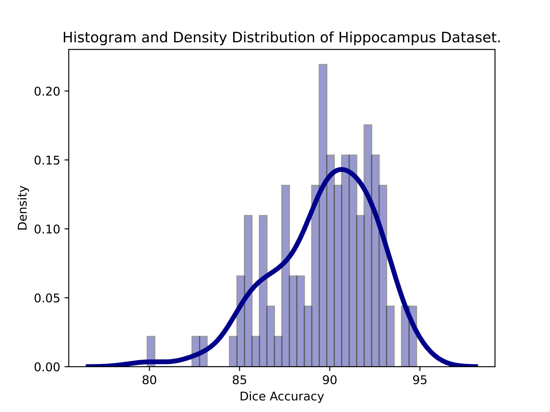
(a)

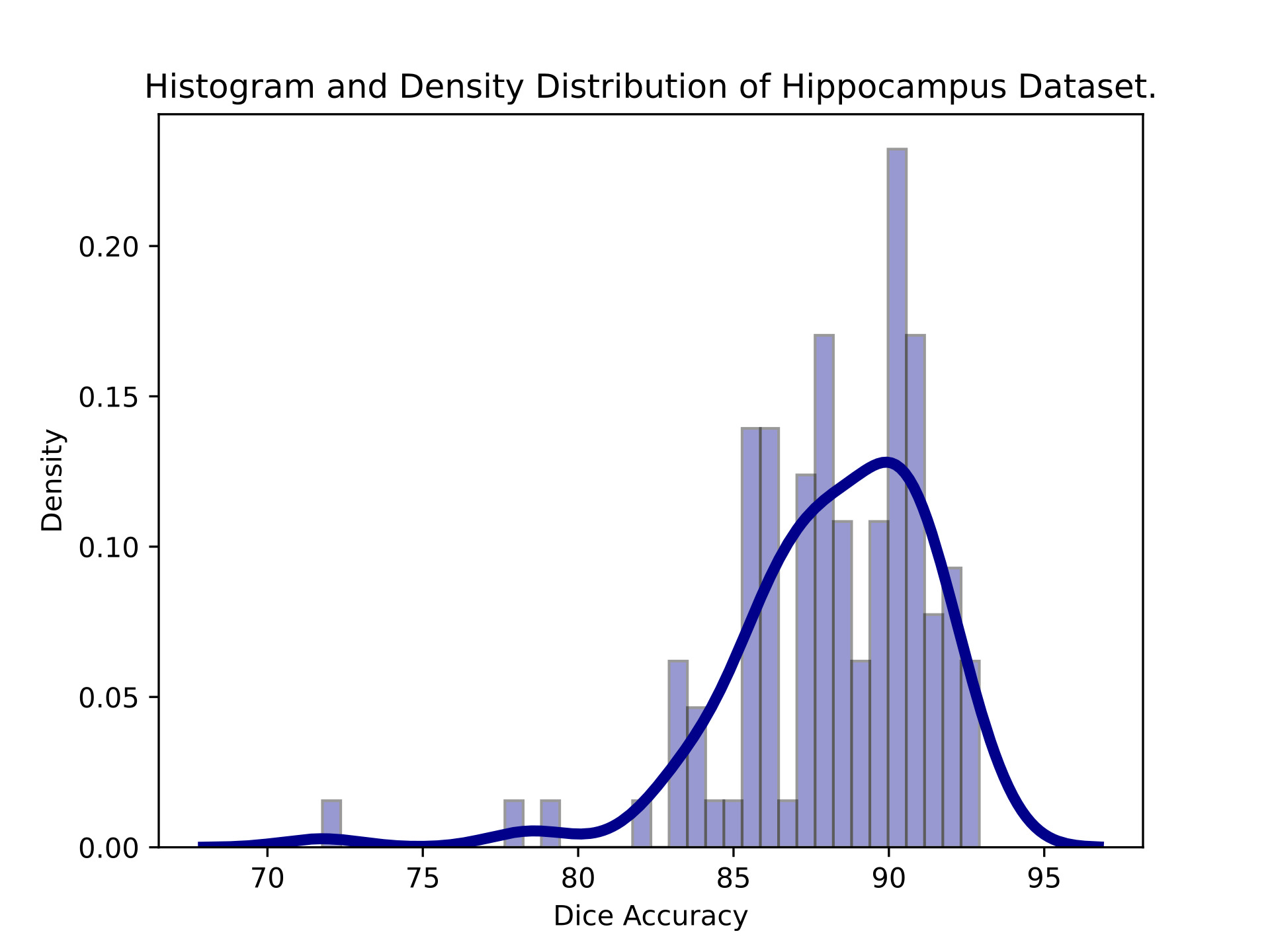
(b)

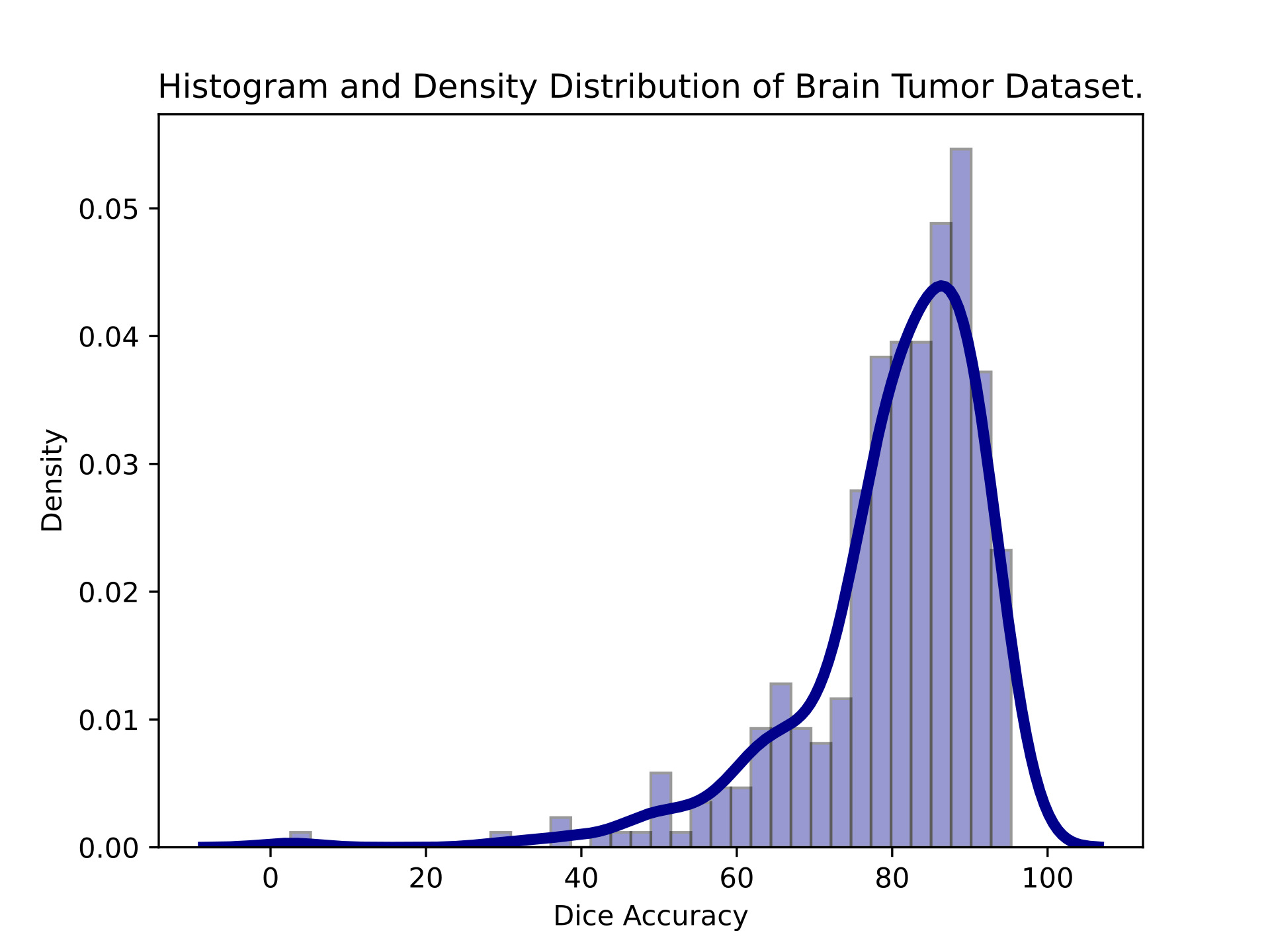
(c)

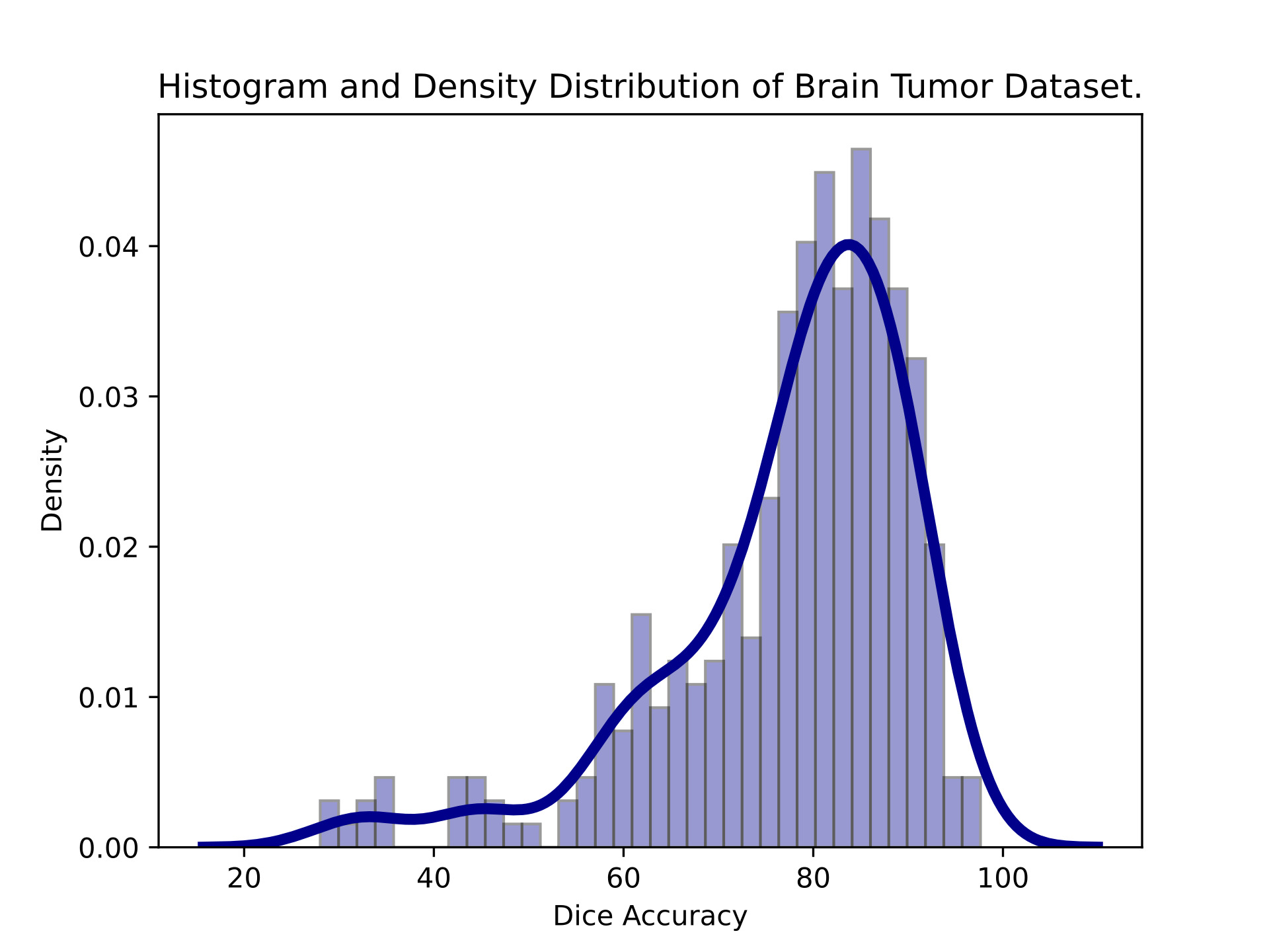
(d)

Figure 1: Histogram of Dice accuracy over the entire test set, shown together with a kernel density estimation (KDE) which smoothes the observations with a Gaussian kernel. (a) Hippocampus dataset, 3D U-Net. (b) Hippocampus dataset, 2D U-Net. (c) Brain Tumor dataset, 3D U-Net. (d) Brain Tumor dataset, 2D U-Net.

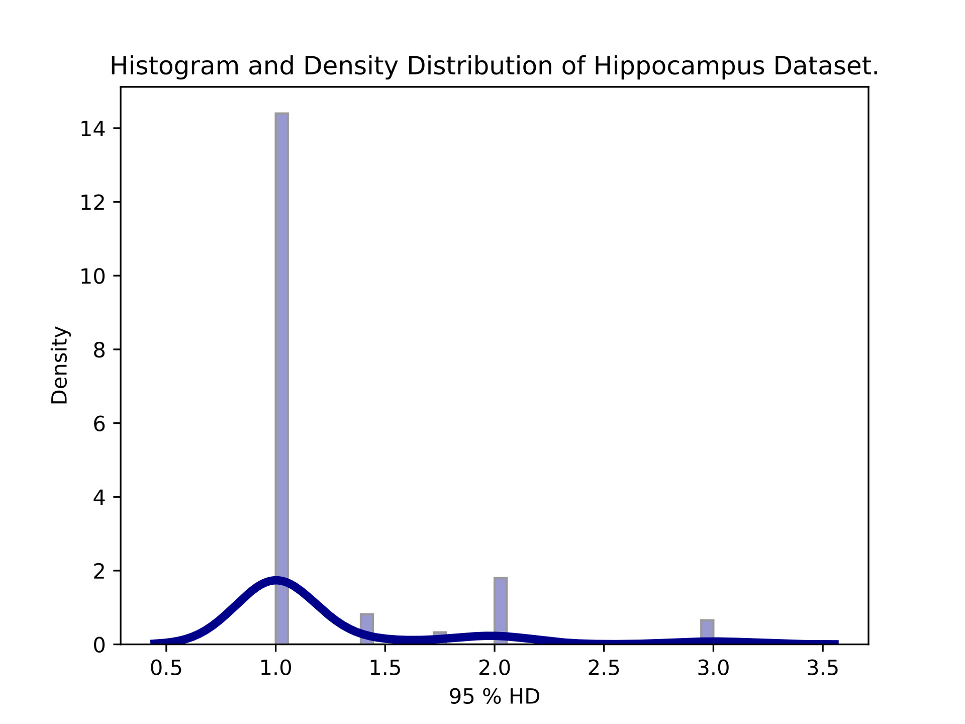
(a)

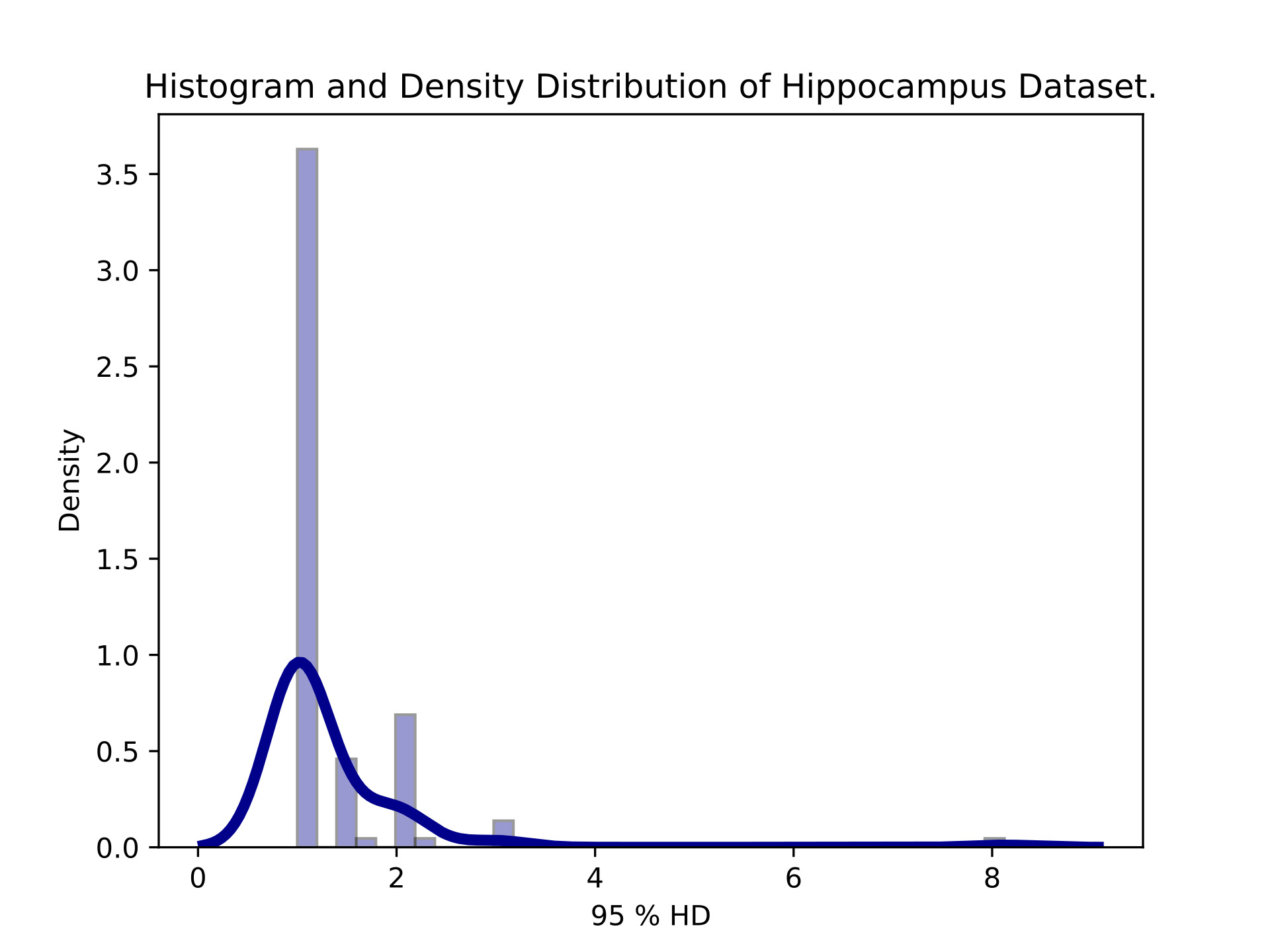
(b)

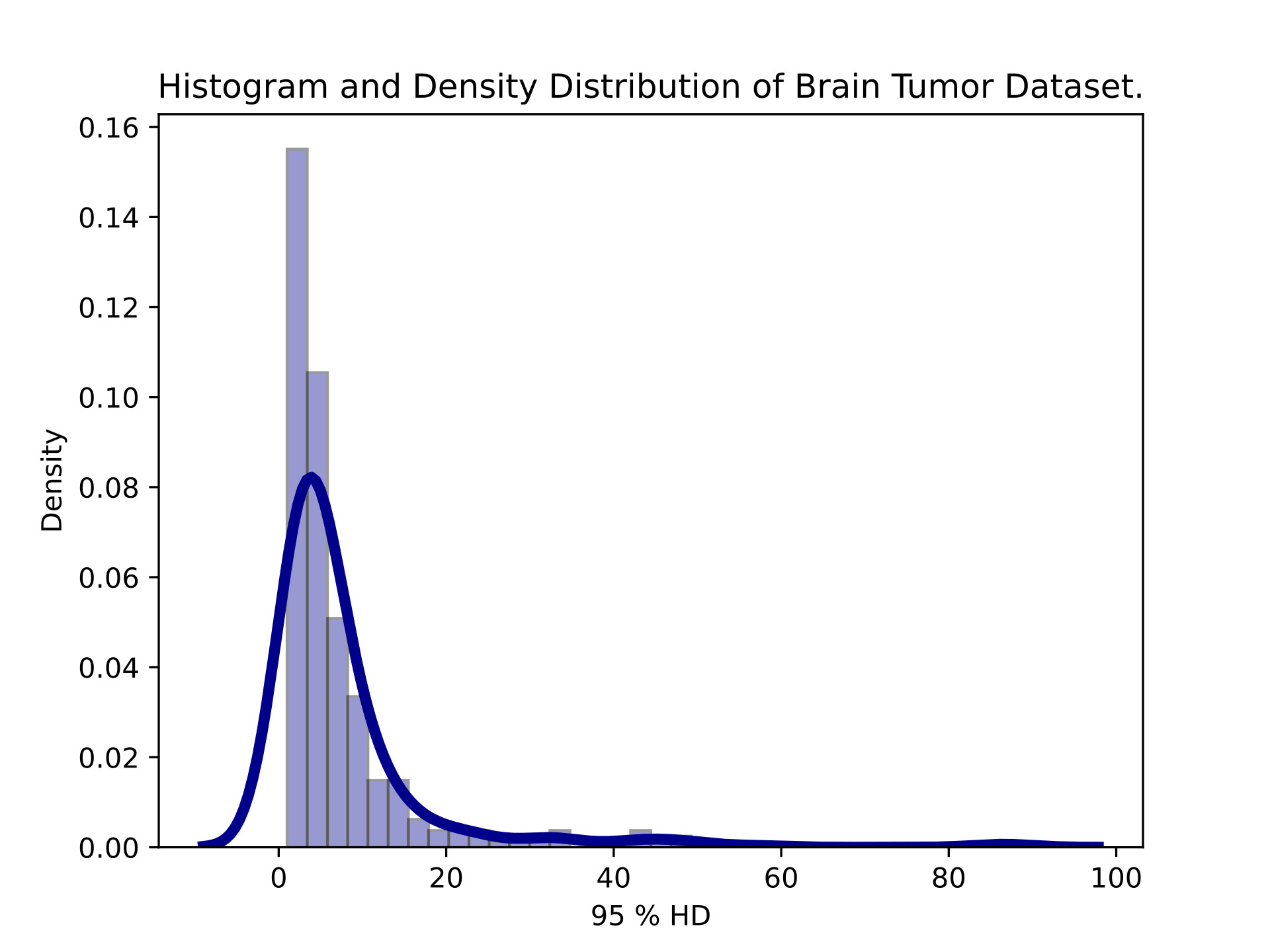
(c)

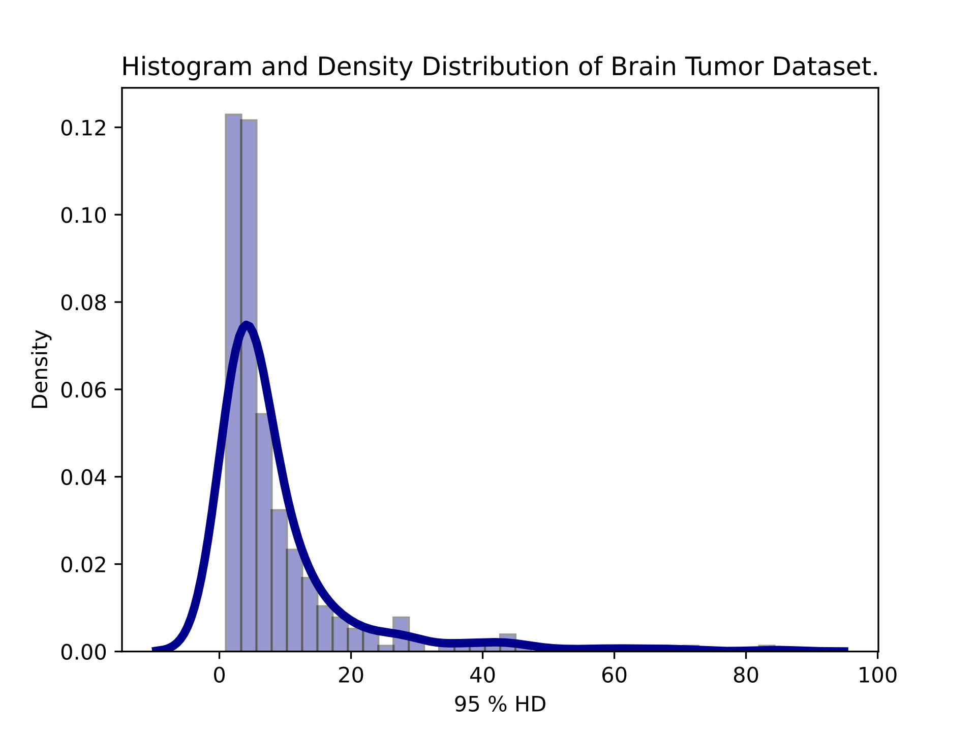
(d)

Figure 2: Histogram of 95% Hausdorff distance over the entire test set, shown together with a kernel density estimation (KDE) which smoothes the observations with a Gaussian kernel. (a) Hippocampus dataset, 3D U-Net. (b) Hippocampus dataset, 2D U-Net. (c) Brain Tumor dataset, 3D U-Net. (d) Brain Tumor dataset, 2D U-Net.

			Parametric					Bootstrap
			$\mu$	$\sigma$	$SEM$	$CI$	$\nu$	$\mu^{*}$	$SEM^{*}$	$CI^{*}$	$\nu^{*}$
Hippocampus	3D U-Net	Dice	89.714	2.797	0.267	[-0.52, 0.52]	0.012	89.715	0.263	[-0.53, 0.51]	0.012
		95 % HD	1.205	0.472	0.045	[-0.08, 0.08]	0.149	1.205	0.045	[-0.08, 0.09]	0.149
($n=110$)	2D U-Net	Dice	88.197	3.267	0.311	[-0.61, 0.61]	0.014	88.199	0.313	[-0.64, 0.59]	0.014
		95% HD	1.311	0.806	0.077	[-0.15, 0.15]	0.229	1.31	0.077	[-0.13, 0.17]	0.229
Brain Tumor	3D U-Net	Dice	80.265	11.947	0.654	[-1.28, 1.28]	0.032	80.268	0.659	[-1.31, 1.24]	0.032
		95 % HD	7.726	10.634	0.582	[-1.14, 1.14]	0.294	7.73	0.581	[-1.08, 1.18]	0.294
($n=334$)	2D U-Net	Dice	$77.489$	$13.115$	$0.718$	[-1.41, 1.41]	0.036	$77.488$	$0.717$	[-1.43, 1.38]	0.036
		95 % HD	8.855	11.262	0.616	[-1.21, 1.21]	0.272	8.862	0.62	[-1.22, 1.22]	0.272

TABLE II: Results on the full test set ($n=110$ for Hippocampus and $n=334$ for Brain Tumor) for region $L_{1}$. $\mu$ and $\sigma$ are the empirical mean and standard deviation of the Dice accuracy (Dice) and 95 % volumetric Hausdorff distance (HD) across all patients in the test set. $SEM$ is the standard error of the mean, $CI$ is the $95\%$ confidence interval independent of the mean calculated using the parametric estimation, $\nu$ is the normalized CI. $\mu^{*}$, $SEM^{*}$, $CI^{*}$ and $\nu^{*}$ are the bootstrap estimates.

IV Experimental Study on the Whole Test Sets

In this section, we study the precision of the performance evaluation using the full test sets (test set sizes are 110 for the Hippocampus and 334 for the Brain Tumor, respectively).

The distribution of Dice accuracy and Hausdorff distance values over the test set are shown in Figure 1. One can observe that the Dice accuracy’s distribution is not very far from Gaussian despite outliers and skewness in the histogram plots. It is not the case for the Hausdorff distance (Figure 2). First, this measure is lower-bounded by one and a lot of values lie to one, which makes the distribution highly skewed. Also, due to the discrete nature of the images, some values will never occur hence histograms are sparse.

We then compute, for both metrics and for both 2D and 3D networks, the test sample mean $\mu$, the test sample standard deviation $\sigma$, SEM, CI and $\nu$. The computations are done as described in Section II, using both parametric and bootstrap estimations. Results are reported in Table II. One can see that, under such test set sizes, the computations using parametric estimation are close to those obtained with the bootstrap, even for the Hausdorff distance. This indicates that it is a reasonable approximation under this size regime. In the next section, we will study if this still holds for smaller test set sizes.

V Experimental Study on Sub-samples of the Test Sets

In this section, we study experimentally the relationship between the test set size and the precision of the estimation of the segmentation performance. To that end, we draw subsamples of variable size

$$k\in K=\{10,20,30,50,100,\ldots,n\}$$

where $n$ is the whole test set size. For the Hippocampus dataset $n=110$ and $K=\{10,20,30,50,100,110\}$ and for the Brain Tumor dataset, $n=334$ and $K=\{10,20,30,50,100,200,300,334\}$.

For small subsamples, the estimates can vary substantially from one drawing to another. In order not to depend on a particular drawing, which may be lucky or unlucky, we repeat the procedure 100 times for each value of $k$. We denote the subsamples as $(S_{k,j})$ where $k$ is the subsample size and $j\in\{1,\ldots,100\}$ is the index of a particular drawing. We then compute the precision measures (SEM, CI, $\nu$ and bootstrap counterparts) for the subsamples of different sizes. The exact formulas for the estimation of the different measures are detailed in appendix -A.

$\sigma\downarrow$	$k\rightarrow$	10	20	30	50	100	200	300	500	1000	1500	2000	2500	3000
0.47	$SEM$	0.15	0.11	0.09	0.07	0.05	0.03	0.03	0.02	0.01	0.01	0.01	0.01	0.01
	$CI$	[-0.29, 0.29]	[-0.21, 0.21]	[-0.17, 0.17]	[-0.13, 0.13]	[-0.09, 0.09]	[-0.07, 0.07]	[-0.05, 0.05]	[-0.04, 0.04]	[-0.03, 0.03]	[-0.02, 0.02]	[-0.02, 0.02]	[-0.02, 0.02]	[-0.02, 0.02]
0.81	$SEM$	0.26	0.18	0.15	0.11	0.08	0.06	0.05	0.04	0.03	0.02	0.02	0.02	0.01
	$CI$	[-0.5, 0.5]	[-0.35, 0.35]	[-0.29, 0.29]	[-0.22, 0.22]	[-0.16, 0.16]	[-0.11, 0.11]	[-0.09, 0.09]	[-0.07, 0.07]	[-0.05, 0.05]	[-0.04, 0.04]	[-0.04, 0.04]	[-0.03, 0.03]	[-0.03, 0.03]
1	$SEM$	0.32	0.22	0.18	0.14	0.1	0.07	0.06	0.04	0.03	0.03	0.02	0.02	0.02
	$CI$	[-0.62, 0.62]	[-0.44, 0.44]	[-0.36, 0.36]	[-0.28, 0.28]	[-0.2, 0.2]	[-0.14, 0.14]	[-0.11, 0.11]	[-0.09, 0.09]	[-0.06, 0.06]	[-0.05, 0.05]	[-0.04, 0.04]	[-0.04, 0.04]	[-0.04, 0.04]
2.79	$SEM$	0.88	0.62	0.51	0.39	0.28	0.2	0.16	0.12	0.09	0.07	0.06	0.06	0.05
	$CI$	[-1.73, 1.73]	[-1.22, 1.22]	[-1.0, 1.0]	[-0.77, 0.77]	[-0.55, 0.55]	[-0.39, 0.39]	[-0.32, 0.32]	[-0.24, 0.24]	[-0.17, 0.17]	[-0.14, 0.14]	[-0.12, 0.12]	[-0.11, 0.11]	[-0.1, 0.1]
3.26	$SEM$	1.03	0.73	0.6	0.46	0.33	0.23	0.19	0.15	0.1	0.08	0.07	0.07	0.06
	$CI$	[-2.02, 2.02]	[-1.43, 1.43]	[-1.17, 1.17]	[-0.9, 0.9]	[-0.64, 0.64]	[-0.45, 0.45]	[-0.37, 0.37]	[-0.29, 0.29]	[-0.2, 0.2]	[-0.16, 0.16]	[-0.14, 0.14]	[-0.13, 0.13]	[-0.12, 0.12]
5	$SEM$	1.58	1.12	0.91	0.71	0.5	0.35	0.29	0.22	0.16	0.13	0.11	0.1	0.09
	$CI$	[-3.1, 3.1]	[-2.19, 2.19]	[-1.79, 1.79]	[-1.39, 1.39]	[-0.98, 0.98]	[-0.69, 0.69]	[-0.57, 0.57]	[-0.44, 0.44]	[-0.31, 0.31]	[-0.25, 0.25]	[-0.22, 0.22]	[-0.2, 0.2]	[-0.18, 0.18]
10.63	$SEM$	3.36	2.38	1.94	1.5	1.06	0.75	0.61	0.48	0.34	0.27	0.24	0.21	0.19
	$CI$	[-6.59, 6.59]	[-4.66, 4.66]	[-3.8, 3.8]	[-2.95, 2.95]	[-2.08, 2.08]	[-1.47, 1.47]	[-1.2, 1.2]	[-0.93, 0.93]	[-0.66, 0.66]	[-0.54, 0.54]	[-0.47, 0.47]	[-0.42, 0.42]	[-0.38, 0.38]
11.26	$SEM$	3.56	2.52	2.06	1.59	1.13	0.8	0.65	0.5	0.36	0.29	0.25	0.23	0.21
	$CI$	[-6.98, 6.98]	[-4.93, 4.93]	[-4.03, 4.03]	[-3.12, 3.12]	[-2.21, 2.21]	[-1.56, 1.56]	[-1.27, 1.27]	[-0.99, 0.99]	[-0.7, 0.7]	[-0.57, 0.57]	[-0.49, 0.49]	[-0.44, 0.44]	[-0.4, 0.4]
12	$SEM$	3.79	2.68	2.19	1.7	1.2	0.85	0.69	0.54	0.38	0.31	0.27	0.24	0.22
	$CI$	[-7.44, 7.44]	[-5.26, 5.26]	[-4.29, 4.29]	[-3.33, 3.33]	[-2.35, 2.35]	[-1.66, 1.66]	[-1.36, 1.36]	[-1.05, 1.05]	[-0.74, 0.74]	[-0.61, 0.61]	[-0.53, 0.53]	[-0.47, 0.47]	[-0.43, 0.43]
13.12	$SEM$	4.15	2.94	2.4	1.86	1.31	0.93	0.76	0.59	0.41	0.34	0.29	0.26	0.24
	$CI$	[-8.13, 8.13]	[-5.75, 5.75]	[-4.69, 4.69]	[-3.64, 3.64]	[-2.57, 2.57]	[-1.82, 1.82]	[-1.48, 1.48]	[-1.15, 1.15]	[-0.81, 0.81]	[-0.66, 0.66]	[-0.58, 0.58]	[-0.51, 0.51]	[-0.47, 0.47]
20	$SEM$	6.32	4.47	3.65	2.83	2.0	1.41	1.15	0.89	0.63	0.52	0.45	0.4	0.37
	$CI$	[-12.4, 12.4]	[-8.77, 8.77]	[-7.16, 7.16]	[-5.54, 5.54]	[-3.92, 3.92]	[-2.77, 2.77]	[-2.26, 2.26]	[-1.75, 1.75]	[-1.24, 1.24]	[-1.01, 1.01]	[-0.88, 0.88]	[-0.78, 0.78]	[-0.72, 0.72]
30	$SEM$	9.49	6.71	5.48	4.24	3.0	2.12	1.73	1.34	0.95	0.77	0.67	0.6	0.55
	$CI$	[-18.59, 18.59]	[-13.15, 13.15]	[-10.74, 10.74]	[-8.32, 8.32]	[-5.88, 5.88]	[-4.16, 4.16]	[-3.39, 3.39]	[-2.63, 2.63]	[-1.86, 1.86]	[-1.52, 1.52]	[-1.31, 1.31]	[-1.18, 1.18]	[-1.07, 1.07]
50	$SEM$	15.81	11.18	9.13	7.07	5.0	3.54	2.89	2.24	1.58	1.29	1.12	1.0	0.91
	$CI$	[-30.99, 30.99]	[-21.91, 21.91]	[-17.89, 17.89]	[-13.86, 13.86]	[-9.8, 9.8]	[-6.93, 6.93]	[-5.66, 5.66]	[-4.38, 4.38]	[-3.1, 3.1]	[-2.53, 2.53]	[-2.19, 2.19]	[-1.96, 1.96]	[-1.79, 1.79]

TABLE III: Table of SEM and confidence intervals $CI$ for different sizes $k$ of the test set and for different values of $\sigma$ including the experimental values obtained in Table II.

V-A Dice Accuracy Performance Measure

Results for the Dice accuracy for different sample sizes $k$ are reported in Figure 3 (details in Tables IV,  V,  VI and  VII). As expected, as the sample size decreases, the estimates become less precise (the standard error increases, the confidence interval widens). Moreover, the confidence intervals obtained via parametric estimation are very close, though slightly below, to the ones obtained via bootstrapping. Overall, since the CI obtained via the parametric estimates are slightly narrower than that of the bootstap values, one can assume that the parametric estimates could serve as a lower bound to the test set size needed to insure a particular precision. Finally, one can observe that bootstrap confidence intervals are slightly skewed. However, this skewness rapidly fades away as the test set sample size $k$ decreases.

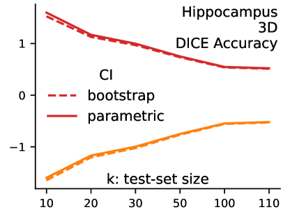
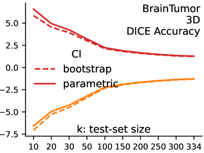
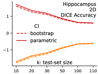
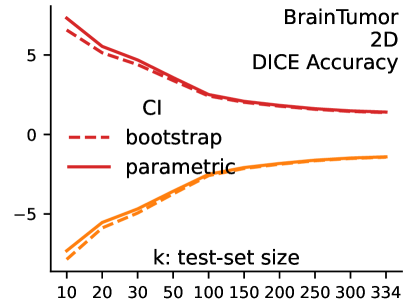
Figure 3: Parametric and boostrap CIs: Dice accuracy (detailed results in Tables IV, V, VI, VII)

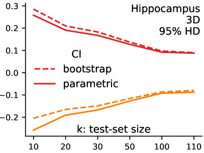
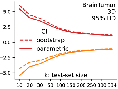
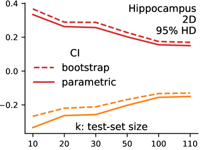
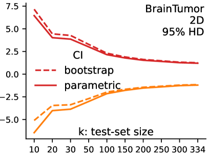
Figure 4: Parametric and boostrap CIs: Hausdorff Distance (detailed results in Tables VIII, IX, X, XI)

V-B Hausdorff Distance Performance Measure

Results for the Hausdorff distance metric are reported in Figure 3 (details in Tables VIII, IX, XI and X). Even though we saw that the Hausdorff distance is far from being Gaussian distributed, it is interesting to note that obtained parametric estimates are actually close to bootstrap ones. It thus seems reasonable to assume that parametric estimates can, as in the case of the Dice accuracy, be used to derive a lower bound on the minimal test set size needed to achieve a given precision.

Inspecting the normalized width $\nu$ (reported in appendix -B) shows that it is much larger for the Hausdorff distance than for the Dice accuracy for the same model and the same dataset. This indicates that more test samples are required to achieve a particular precision. Possible explanations include the discontinuity of the Hausdorff distance and the fact that it corresponds to a maximum rather than an average.

VI A table of Gaussian confidence intervals

The previous section shows that parametric estimates match well bootstrap confidence intervals. Confidence intervals can be useful even before running an experiment, to give a lower bound for the dataset size needed to achieve a given precision. To facilitate the use of confidence intervals, Table III list them for different values of test set size $k$ and $\sigma$ (which reflects how variable is the performance across test samples), computed via Equations 1. Some values of $\sigma$ match those experimentally measured in our experiences in Table II (0.47, 0.81, 2.79, 3.26, 10.63, 11.26, 13.12). We recall that the value of $\mu$, in itself, has no impact on the width of the confidence interval nor on the SEM –even though it is usually observed that lower performing models, thus associated with a lower value of $\mu$, also have a more variable performance and thus a larger value of $\sigma$.

VII Discussion

We have studied the precision with which segmentation performance can be estimated in typical medical imaging studies. We provided typical values for confidence intervals of the performance of trained models. Such values can be useful to authors and reviewers, e.g. to roughly estimate confidence intervals that can be expected for a given study. Finally, we have shown that, under typical performance spreads, the sample size needed to achieve a given confidence interval is smaller than for classification tasks. To that purpose, we have conducted an extensive set of experiments using both parametric and bootstrap estimates. Results show that parametric estimates give reasonable results even when the performance metric substantially deviates from a Gaussian distribution.

Confidence intervals cannot be computed post-hoc

The width of the confidence interval depends on two factors: the size of the test set ($n$) and the variability of the performance ($\sigma$). In classification, a binomial distribution gives parametric confidence intervals –though slightly conservative [10, 11]. Confidence intervals can be computed post-hoc as a function of the accuracy, e.g. when reading a manuscript. This is not the case in image segmentation: for a given metric, $\sigma$ is highly task dependent and not directly linked to the performance (in practice, lower performing models are often associated to higher standard deviations). Hence, $\sigma$ must be computed during model evaluation, and studies should report confidence intervals and potentially $\sigma$.

A table for confidence intervals

As parametric estimates give reasonable results, one can compute typical confidence intervals for given $n$ and $\sigma$ and we provide this information in Table III. These values can be useful to researchers preparing a segmentation study, to help them choose the size of the test set. Investigators must then make an hypothesis on the expected value of $\sigma$ (as when doing a power analysis), for example using previously published studies on similar segmentation tasks (given that these report $\sigma$). The values can also be useful to reviewers who can use these to gauge plausible confidence intervals, should these not be reported in the paper. Again, if $\sigma$ is not reported in the paper, one will need to make an hypothesis on its expected value.

Test-set size for statistical control

Classification tasks need large test-set sizes for tight confidence intervals (though higher-performing models lead to less uncertainty). Typically, for classification a 1%-wide confidence interval requires about $10\,000$ samples for models with over 90% accuracy [11].

Our results show that the typical test size needed for a given confidence interval is smaller for segmentation than for classification. This is good news as it is arguably more difficult to obtain a large test set in the case of segmentation as it requires voxel-wise annotation by a trained rater. However, smaller does not mean small. When dispersion is low ($\sigma\leq 3$ for Dice accuracy), hundreds of samples may suffice for tight confidence intervals (e.g. 1%-wide). When the dispersion is larger (for example $\sigma\approx 15$), as often for more difficult tasks, a $1\%$-wide confidence interval may require more than 1 000 test samples. More relaxed confidence intervals (e.g. $4\%$-wide) may still require about 200 test samples.

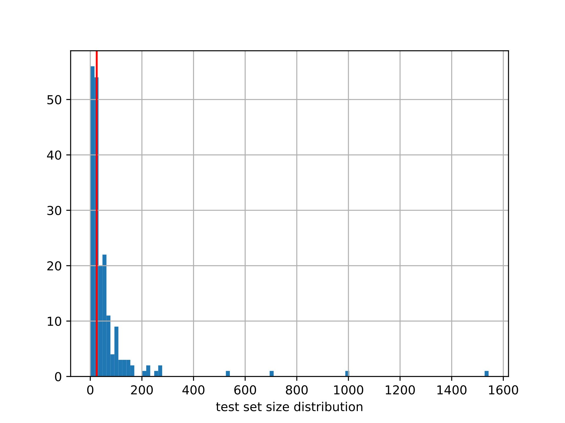
Figure 5: Histogram of the test-set size of different experiments from segmentation papers published in JMI, TMI, and MedIA in 2022. The red line represents the median test size ($n=25$).

A call for larger test sets

Are the practices of medical-imaging studies in line with such test set sizes? As mentioned in the introduction, we surveyed papers published in 2022 in three medical imaging journals: IEEE Transactions on Medical Imaging (IEEE TMI), Medical Image Analysis (MedIA), and SPIE’s Journal of Medical Imaging (JMI) dealing with segmentation of 3D images. This survey, though not exhaustive, sheds light on current practices in recent medical-imaging papers. Figure 5 shows that the test set size is in general small and highly variable across studies (median, 25; minimum: 1; maximum: 1543). Thus, with the exception of a few studies, there is a need to increase the size of test sets to obtain reasonably precise estimates of the performance.

Reporting confidence intervals is important

Trustworthy evidence on segmentation tools is important for their clinical adoption. Confidence intervals and bootstrapping are classic statistical practice; and yet medical image segmentation papers seldom report confidence intervals: we found them in only 10% of papers of our survey (Table I). Beyond immediate clinical adoption, controlled statistical evidence is a component of reproducibility, needed for scientific progress [18, 19]. Statistical reproducibility is suited to reason on generalization to unseen data: results need to be statistically compatible rather than identical. Reporting confidence intervals is central to asserting statistical reproducibility of studies. Awareness about this issue has risen, as can been seen for example in reproducibility checklists (e.g. MICCAI 2021). However, the fact that confidence intervals are so rarely reported in recent papers indicates yet more awareness is needed.

Reporting confidence intervals enables progress at the level of the community. To disseminate a trained model (for use by clinical researchers, neuroscientists …), the users should understand expected variances in the performance of the model. Confidence intervals also enable comparing performance to inter-rater (or intra-rater) variability. When computing inter-rater variability on the test set used to evaluate the trained model, one can obtain confidence intervals for the trained model and for the inter-rater and check if they overlap.

Recommendations

We recommend that authors systematically report confidence intervals for trained models. Even though we showed that parametric approximations can yield reasonable estimates, we recommend to use the bootstrap method as it makes much fewer assumptions and is easy to perform since it only requires to resample performance metrics obtained on the test set (without recomputing them). Finally, confidence intervals should be complemented by displaying the distribution of the performance metrics (e.g. as a violin plot or a box plot) on the test set and reporting its standard deviation.

More work to benchmark learning procedures

We investigated the sampling noise in the test set, the only source of variance when evaluating a trained model. However evaluating a learning procedure –as when comparing two methods– comes with other sources of variance such as hyperparameters or random seeds [20, 11]. Methods to build confidence intervals for learning procedures typically involve running multiple trainings with different data splits (to account for sampling noise in training and testing sets) but also different hyperparameters or random seeds [20, 11]. They require much more computing power and lead to wider confidence intervals.

Limitations

While we studied the two most widely used performance metrics, there are many other metrics, some being more appropriate for certain settings [3]. Also, due to space constraints, we only studied two datasets. We have chosen them to include both a relatively easy and a more difficult segmentation task. However, conducting similar experiments on other datasets would be ground for more general conclusions.

VIII Conclusion

Confidence intervals are needed to characterize the uncertainty on the performance of image-segmentation tools. We have shown that simple parametric estimates can serve as a reasonable reference to guide researchers on the test set size needed for a target precision. Importantly, results show that the test set size needed to achieve a given precision is lower for segmentation than for classification tasks. Confidence intervals can be computed easily; we hope that they will be used more in image-segmentation studies.

-A Details on the estimated measures on subsamples of the test sets

Parametric estimates

For the parametric estimation, we denote as

$$\mu_{k,j}=\frac{1}{k}\sum_{l=1}^{k}P_{j,k,l},\quad\sigma_{k,j}=\sqrt{\frac{1}{k}\sum_{l=1}^{k}{\left(P_{j,k,l}-\mu_{k,j}\right)^{2}}}$$

the empirical mean and standard deviation for the subsample $S_{k,j}$ where $P_{j,k,l}$ is the performance metric (in our case either Dice accuracy or Hausdorff distance) of a given subject in the sub-sample $S_{k,j}$. Similarly, we use the notations

$$\text{SEM}_{k,j}=\frac{\sigma_{k,j}}{\sqrt{k}},\quad\nu_{k,j}=\frac{2*1.96*\text{SEM}_{k,j}}{\mu_{k,j}}.$$

We then compute the average of $\mu_{k,j}$, $\sigma_{k,j}$, $\text{SEM}_{k,j}$, $\nu_{k,j}$ across the different subsamples $S_{k,j}$ for $k$ fixed and $j\in\{1,\ldots,100\}$. This provides the following estimates $\mu_{k}$, $\sigma_{k}$, $\text{SEM}_{k}$ and $\nu_{k}$. Similarly, we define $\text{CI}_{k}=[-1.96\times\text{SEM}_{k},1.96\times\text{SEM}_{k}]$.

Bootstrap estimates

Bootstrap estimations are performed as follows. For a given subsample $S_{k,j}$ of size $k$ and index $j$, $M=15\,000$ bootstrap samples of size $k$ are drawn with replacement. We denote a given bootstrap sample as $S^{*}_{k,j,m}$ and its mean as $\mu^{*}_{k,j,m}$ where $m\in\{1,\ldots,M\}$ is the index of the $m^{th}$ bootstrap sample of subsample $S_{k,j}$. The bootstrap mean $\mu^{*}_{k,j}$ of $S_{k,j}$ is the mean of the bootstrap sample means $\mu^{*}_{k,j,m}$:

$$\mu^{*}_{k,j}=\frac{1}{M}\sum_{m=1}\mu^{*}_{k,j,m}$$

The standard error of the mean $\mu^{*}_{k,j}$ (denoted as $\text{SEM}^{*}_{k,j}$) obtained via bootstrapping is the standard deviation of the means of all bootstrap samples of subsample $S_{k,j}$:

$$\text{SEM}^{*}_{k,j}=\sqrt{\frac{1}{M}\sum_{m=1}^{M}{\left(\mu^{*}_{k,j,m}-\mu^{*}_{k,j}\right)^{2}}}.$$

The $95\%$ confidence interval of the sample $S_{k,j}$ is denoted as $[a^{*}_{k,j},b^{*}_{k,j}]$ and is the set of values between the $2.5\%$ and $97.5\%$ percentile of the sorted bootstrap means of subsample $S_{k,j}$. We then compute the average of $\mu^{*}_{k,j}$, and $\text{SEM}^{*}_{k,j}$ across the different subsamples $S_{k,j}$ for $k$ fixed and $j\in\{1,...,100\}$ and denote the results as $\mu^{*}_{k}$ and $\text{SEM}^{*}_{k}$. For the confidence intervals, we compute the average values $a^{*}_{k}=\frac{1}{100}\sum_{j=1}^{100}{a^{*}_{k,j}}$ and $b^{*}_{k}=\frac{1}{100}\sum_{j=1}^{100}{b^{*}_{k,j}}$ to obtain the average confidence interval independent of the mean $\text{CI}^{*}_{k}=[a^{*}_{k}-\mu^{*}_{k},b^{*}_{k}-\mu^{*}_{k}]$. We finally compute the normalized width of the confidence interval as: $\nu^{*}_{k}=\frac{b^{*}_{k}-a^{*}_{k}}{\mu^{*}_{k}}$.

-B Detailed results on subsamples of the test sets

Detailed results on subsamples of the test set, which were summarized in Figures 3 and 4, are presented in Tables IV, V, VI, VII, VIII, IX, X and XI.

	Parametric					Bootstrap
Subsample size $k$	$\mu_{k}$	$\sigma_{k}$	$SEM_{k}$	$CI_{k}$	$\nu_{k}$	$\mu^{*}_{k}$	$SEM^{*}_{k}$	$CI^{*}_{k}$	$\nu^{*}_{k}$
10	$89.751$	$2.578$	$0.815$	[-1.6, 1.6]	0.036	$89.752$	$0.815$	$[-1.647,1.525]$	0.035
20	$89.723$	$2.666$	$0.596$	[-1.17, 1.17]	0.026	$89.724$	$0.597$	$[-1.204,1.128]$	0.026
30	$89.681$	$2.785$	$0.508$	[-0.995, 0.995]	0.022	$89.682$	$0.508$	$[-1.023,0.968]$	0.022
50	$89.768$	$2.707$	$0.383$	[-0.75, 0.75]	0.017	$89.768$	$0.383$	$[-0.766,0.734]$	0.017
100	$89.721$	$2.788$	$0.279$	[-0.545, 0.545]	0.012	$89.721$	$0.279$	$[-0.557,0.536]$	0.012
110	$89.714$	$2.784$	$0.265$	[-0.52, 0.52]	0.012	$89.714$	$0.266$	$[-0.529,0.512]$	0.012

TABLE IV: Hippocampus dataset, 3D U-net, Dice accuracy. Results on sub-samples of size $k\leq 110$. We show the mean over all the sub-samples $S_{k,j}$ of a given size $k$ ($k$ is fixed and $j\in\{1,\ldots,100\}$).

	Parametric					Bootstrap
Subsample size $k$	$\mu_{k}$	$\sigma_{k}$	$SEM_{k}$	$CI_{k}$	$\nu_{k}$	$\mu^{*}_{k}$	$SEM^{*}_{k}$	$CI^{*}_{k}$	$\nu^{*}_{k}$
10	$88.334$	$2.759$	$0.872$	[-1.71, 1.71]	0.039	$88.335$	$0.872$	$[-1.78,1.608]$	0.038
20	$88.189$	$3.082$	$0.689$	[-1.35, 1.35]	0.031	$88.19$	$0.689$	$[-1.425,1.263]$	0.030
30	$88.126$	$3.281$	$0.599$	[-1.175, 1.175]	0.027	$88.126$	$0.599$	$[-1.24,1.102]$	0.027
50	$88.254$	$3.12$	$0.441$	[-0.865, 0.865]	0.020	$88.255$	$0.441$	$[-0.905,0.822]$	0.020
100	$88.212$	$3.261$	$0.326$	[-0.64, 0.64]	0.015	$88.212$	$0.326$	$[-0.664,0.612]$	0.014
110	$88.197$	$3.252$	$0.31$	[-0.61, 0.61]	0.014	$88.197$	$0.31$	$[-0.631,0.584]$	0.014

TABLE V: Hippocampus dataset, 2D U-net, Dice Accuracy. Results on subsamples of size $k\leq 110$. We show the mean over all the sub-samples $S_{k,j}$ of a given size $k$ ($k$ is fixed and $j\in\{1,\ldots,100\}$).

	Parametric					Bootstrap
Subsample size $k$	$\mu_{k}$	$\sigma_{k}$	$SEM_{k}$	$CI_{k}$	$\nu_{k}$	$\mu^{*}_{k}$	$SEM^{*}_{k}$	$CI^{*}_{k}$	$\nu^{*}_{k}$
10	$80.457$	$10.612$	$3.356$	[-6.58, 6.58]	0.164	$80.461$	$3.356$	$[-7.051,5.853]$	0.160
20	$80.188$	$11.281$	$2.522$	[-4.945, 4.945]	0.123	$80.189$	$2.523$	$[-5.28,4.541]$	0.122
30	$79.925$	$11.839$	$2.162$	[-4.235, 4.235]	0.106	$79.924$	$2.162$	$[-4.512,3.925]$	0.106
50	$80.375$	$11.593$	$1.64$	[-3.215, 3.215]	0.080	$80.374$	$1.639$	$[-3.384,3.015]$	0.080
100	$80.388$	$11.389$	$1.139$	[-2.23, 2.23]	0.055	$80.388$	$1.139$	$[-2.321,2.137]$	0.055
150	$80.329$	$11.788$	$0.962$	[-1.885, 1.885]	0.047	$80.328$	$0.963$	$[-1.954,1.817]$	0.047
200	$80.253$	$11.936$	$0.844$	[-1.655, 1.655]	0.041	$80.252$	$0.844$	$[-1.709,1.601]$	0.041
250	$80.295$	$11.919$	$0.754$	[-1.475, 1.475]	0.037	$80.296$	$0.754$	$[-1.521,1.431]$	0.037
300	$80.28$	$11.924$	$0.688$	[-1.35, 1.35]	0.034	$80.281$	$0.688$	$[-1.386,1.311]$	0.034
334	$80.265$	$11.929$	$0.653$	[-1.28, 1.28]	0.032	$80.264$	$0.653$	$[-1.313,1.245]$	0.032

TABLE VI: Brain Tumor dataset, 3D U-net, Dice Accuracy. Results on subsamples of size $k\leq 334$. We show the mean over all the sub-samples $S_{k,j}$ of a given size $k$ ($k$ is fixed and $j\in\{1,\ldots,100\}$).

	Parametric					Bootstrap
Subsample size $k$	$\mu_{k}$	$\sigma_{k}$	$SEM_{k}$	$CI_{k}$	$\nu_{k}$	$\mu^{*}_{k}$	$SEM^{*}_{k}$	$CI^{*}_{k}$	$\nu^{*}_{k}$
10	$77.811$	$11.799$	$3.731$	[-7.315, 7.315]	0.188	$77.815$	$3.731$	$[-7.856,6.566]$	0.185
20	$77.334$	$12.631$	$2.824$	[-5.535, 5.535]	0.143	$77.334$	$2.825$	$[-5.879,5.137]$	0.142
30	$77.101$	$13.084$	$2.389$	[-4.68, 4.68]	0.121	$77.101$	$2.389$	$[-4.94,4.389]$	0.121
50	$77.607$	$12.897$	$1.824$	[-3.575, 3.575]	0.092	$77.606$	$1.823$	$[-3.736,3.39]$	0.092
100	$77.564$	$12.797$	$1.28$	[-2.51, 2.51]	0.065	$77.564$	$1.279$	$[-2.588,2.42]$	0.065
150	$77.583$	$13.01$	$1.062$	[-2.08, 2.08]	0.054	$77.582$	$1.063$	$[-2.139,2.023]$	0.054
200	$77.468$	$13.182$	$0.932$	[-1.825, 1.825]	0.047	$77.467$	$0.932$	$[-1.871,1.778]$	0.047
250	$77.549$	$13.056$	$0.826$	[-1.62, 1.62]	0.042	$77.549$	$0.826$	$[-1.654,1.582]$	0.042
300	$77.501$	$13.104$	$0.757$	[-1.485, 1.485]	0.038	$77.502$	$0.756$	$[-1.511,1.448]$	0.038
334	$77.489$	$13.115$	$0.718$	[-1.405, 1.405]	0.036	$77.488$	$0.717$	$[-1.43,1.376]$	0.036

TABLE VII: Brain Tumor dataset, 2D U-net, Dice Accuracy. Results on subsamples of size $k\leq 334$. We show the mean over all the sub-samples $S_{k,j}$ of a given size $k$ ($k$ is fixed and $j\in\{1,\ldots,100\}$).

	Parametric					Bootstrap
Subsample size $k$	$\mu_{k}$	$\sigma_{k}$	$SEM_{k}$	$CI_{k}$	$\nu_{k}$	$\mu^{*}_{k}$	$SEM^{*}_{k}$	$CI^{*}_{k}$	$\nu^{*}_{k}$
10	$1.214$	$0.416$	$0.132$	[-0.26, 0.26]	0.428	$1.214$	$0.131$	$[-0.205,0.286]$	0.404
20	$1.206$	$0.435$	$0.097$	[-0.19, 0.19]	0.315	$1.206$	$0.097$	$[-0.165,0.21]$	0.310
30	$1.221$	$0.468$	$0.086$	[-0.17, 0.17]	0.278	$1.22$	$0.086$	$[-0.149,0.183]$	0.271
50	$1.203$	$0.46$	$0.065$	[-0.125, 0.125]	0.208	$1.203$	$0.065$	$[-0.116,0.137]$	0.211
100	$1.205$	$0.47$	$0.047$	[-0.09, 0.09]	0.149	$1.205$	$0.047$	$[-0.086,0.097]$	0.152
110	$1.205$	$0.47$	$0.045$	[-0.09, 0.09]	0.149	$1.205$	$0.045$	$[-0.08,0.09]$	0.149

TABLE VIII: Hippocampus dataset, 3D U-net, Hausdorff Distance. Results on sub-samples of size $k\leq 110$. We show the mean over all the sub-samples $S_{k,j}$ of a given size $k$ ($k$ is fixed and $j\in\{1,\ldots,100\}$).

	Parametric					Bootstrap
Subsample size $k$	$\mu_{k}$	$\sigma_{k}$	$SEM_{k}$	$CI_{k}$	$\nu_{k}$	$\mu^{*}_{k}$	$SEM^{*}_{k}$	$CI^{*}_{k}$	$\nu^{*}_{k}$
10	$1.296$	$0.538$	$0.17$	[-0.335, 0.335]	0.517	$1.296$	$0.17$	$[-0.267,0.367]$	0.490
20	$1.302$	$0.599$	$0.134$	[-0.265, 0.265]	0.407	$1.302$	$0.134$	$[-0.219,0.289]$	0.391
30	$1.331$	$0.718$	$0.131$	[-0.255, 0.255]	0.383	$1.331$	$0.131$	$[-0.211,0.288]$	0.375
50	$1.31$	$0.729$	$0.103$	[-0.2, 0.2]	0.305	$1.31$	$0.103$	$[-0.168,0.228]$	0.303
100	$1.31$	$0.793$	$0.079$	[-0.155, 0.155]	0.237	$1.31$	$0.079$	$[-0.133,0.175]$	0.234
110	$1.311$	$0.803$	$0.077$	[-0.15, 0.15]	0.229	$1.311$	$0.077$	$[-0.13,0.17]$	0.229

TABLE IX: Hippocampus dataset, 2D U-net, Hausdorff Distance. Results on subsamples of size $k\leq 110$. We show the mean over all the sub-samples $S_{k,j}$ of a given size $k$ ($k$ is fixed and $j\in\{1,\ldots,100\}$).

	Parametric					Bootstrap
Subsample size $k$	$\mu_{k}$	$\sigma_{k}$	$SEM_{k}$	$CI_{k}$	$\nu_{k}$	$\mu^{*}_{k}$	$SEM^{*}_{k}$	$CI^{*}_{k}$	$\nu^{*}_{k}$
10	$8.171$	$8.806$	$2.785$	[-5.46, 5.46]	1.336	$8.168$	$2.784$	$[-4.278,6.046]$	1.264
20	$7.635$	$9.098$	$2.034$	[-3.985, 3.985]	1.044	$7.634$	$2.034$	$[-3.268,4.459]$	1.012
30	$7.95$	$9.782$	$1.786$	[-3.5, 3.5]	0.881	$7.95$	$1.787$	$[-2.98,3.909]$	0.866
50	$7.563$	$9.791$	$1.385$	[-2.715, 2.715]	0.718	$7.563$	$1.383$	$[-2.36,3.002]$	0.709
100	$7.702$	$10.468$	$1.047$	[-2.05, 2.05]	0.532	$7.702$	$1.046$	$[-1.848,2.228]$	0.529
150	$7.691$	$10.339$	$0.844$	[-1.655, 1.655]	0.430	$7.693$	$0.844$	$[-1.522,1.775]$	0.428
200	$7.698$	$10.413$	$0.736$	[-1.445, 1.445]	0.375	$7.697$	$0.736$	$[-1.341,1.535]$	0.374
250	$7.758$	$10.663$	$0.674$	[-1.32, 1.32]	0.340	$7.757$	$0.674$	$[-1.238,1.397]$	0.340
300	$7.695$	$10.513$	$0.607$	[-1.19, 1.19]	0.309	$7.694$	$0.607$	$[-1.12,1.257]$	0.309
334	$7.726$	$10.618$	$0.581$	[-1.14, 1.14]	0.295	$7.726$	$0.581$	$[-1.076,1.196]$	0.294

TABLE X: Brain Tumor dataset, 3D U-net, Hausdorff Distance. Results on subsamples of size $k\leq 334$. We show the mean over all the sub-samples $S_{k,j}$ of a given size $k$ ($k$ is fixed and $j\in\{1,\ldots,100\}$).

	Parametric					Bootstrap
Subsample size $k$	$\mu_{k}$	$\sigma_{k}$	$SEM_{k}$	$CI_{k}$	$\nu_{k}$	$\mu^{*}_{k}$	$SEM^{*}_{k}$	$CI^{*}_{k}$	$\nu^{*}_{k}$
10	$9.544$	$10.409$	$3.292$	[-6.45, 6.45]	1.352	$9.544\pm 3.441$	$3.294$	$[-5.099,7.152]$	1.284
20	$8.454$	$9.178$	$2.052$	[-4.02, 4.02]	0.951	$8.453\pm 2.302$	$2.05$	$[-3.454,4.441]$	0.934
30	$9.204$	$10.794$	$1.971$	[-3.86, 3.86]	0.839	$9.205\pm 1.786$	$1.973$	$[-3.374,4.269]$	0.830
50	$8.836$	$10.86$	$1.536$	[-3.01, 3.01]	0.681	$8.837\pm 1.359$	$1.537$	$[-2.696,3.282]$	0.676
100	$8.758$	$10.966$	$1.097$	[-2.15, 2.15]	0.491	$8.756\pm 0.938$	$1.096$	$[-1.974,2.307]$	0.489
150	$8.886$	$11.158$	$0.911$	[-1.785, 1.785]	0.402	$8.885\pm 0.673$	$0.912$	$[-1.671,1.894]$	0.401
200	$8.806$	$11.068$	$0.783$	[-1.535, 1.535]	0.349	$8.806\pm 0.471$	$0.783$	$[-1.445,1.617]$	0.348
250	$8.873$	$11.32$	$0.716$	[-1.405, 1.405]	0.317	$8.873\pm 0.357$	$0.715$	$[-1.33,1.469]$	0.315
300	$8.83$	$11.173$	$0.645$	[-1.265, 1.265]	0.287	$8.831\pm 0.214$	$0.645$	$[-1.204,1.32]$	0.286
334	$8.855$	$11.245$	$0.615$	[-1.205, 1.205]	0.272	$8.856$	$0.615$	$[-1.154,1.257]$	0.272

TABLE XI: Brain Tumor dataset, 2D U-net, Hausdorff Distance. Results on sub-samples of size $k\leq 334$. We show the mean over all the sub-samples $S_{k,j}$ of a given size $k$ ($k$ is fixed and $j\in\{1,\ldots,100\}$).

References

- [1] M. H. Hesamian, W. Jia, X. He, and P. Kennedy, “Deep learning techniques for medical image segmentation: achievements and challenges,” Journal of digital imaging, vol. 32, pp. 582–596, 2019.
- [2] A. Reinke, E. Christodoulou, B. Glocker, P. Scholz, F. Isensee, and et al, “Metrics reloaded - a new recommendation framework for biomedical image analysis validation,” in Medical Imaging with Deep Learning, 2022. [Online]. Available: https://openreview.net/forum?id=24kBqy8rcB_
- [3] L. Maier-Hein, A. Reinke, P. Godau, M. D. Tizabi, E. Christodoulou, B. Glocker, and et al, “Metrics reloaded: Pitfalls and recommendations for image analysis validation,” arXiv preprint, vol. arXiv:2206.01653, 2022. [Online]. Available: https://arxiv.org/abs/2206.01653
- [4] A. Reinke, M. D. Tizabi, M. Baumgartner, M. Eisenmann, D. Heckmann-Nötzel, A. E. Kavu, T. Rädsch, C. H. Sudre, L. Acion, M. Antonelli et al., “Understanding metric-related pitfalls in image analysis validation,” arXiv preprint arXiv:2302.01790, 2023. [Online]. Available: https://arxiv.org/abs/2302.01790
- [5] L. Maier-Hein, M. Eisenmann, A. Reinke, S. Onogur, M. Stankovic, P. Scholz, T. Arbel, H. Bogunovic, A. P. Bradley, A. Carass et al., “Why rankings of biomedical image analysis competitions should be interpreted with care,” Nature communications, vol. 9, no. 1, p. 5217, 2018.
- [6] G. Varoquaux and V. Cheplygina, “Machine learning for medical imaging: methodological failures and recommendations for the future,” NPJ digital medicine, vol. 5, no. 1, p. 48, 2022.
- [7] M. Chupin, E. Gérardin, R. Cuingnet, C. Boutet, L. Lemieux, S. Lehéricy, H. Benali, L. Garnero, and O. Colliot, “Fully automatic hippocampus segmentation and classification in Alzheimer’s disease and mild cognitive impairment applied on data from ADNI,” Hippocampus, vol. 19, no. 6, pp. 579–587, 2009.
- [8] T. Samaille, L. Fillon, R. Cuingnet, E. Jouvent, H. Chabriat, D. Dormont, O. Colliot, and M. Chupin, “Contrast-based fully automatic segmentation of white matter hyperintensities: method and validation,” PLoS one, vol. 7, no. 11, p. e48953, 2012.
- [9] R. El Jurdi, C. Petitjean, P. Honeine, V. Cheplygina, and F. Abdallah, “A surprisingly effective perimeter-based loss for medical image segmentation,” in Medical Imaging with Deep Learning, 2021, pp. 158–167.
- [10] G. Varoquaux, “Cross-validation failure: Small sample sizes lead to large error bars,” NeuroImage, vol. 180, pp. 68–77, 2018.
- [11] G. Varoquaux and O. Colliot, “Evaluating machine learning models and their diagnostic value,” HAL preprint, vol. hal-03682454, 2022. [Online]. Available: https://hal.archives-ouvertes.fr/hal-03682454
- [12] F. Isensee, P. F. Jaeger, S. A. A. Kohl, J. Petersen, and K. H. Maier-Hein, “nnU-Net: a self-configuring method for deep learning-based biomedical image segmentation,” Nature Methods, vol. 18, no. 2, pp. 203–211, Feb 2021.
- [13] M. Antonelli, A. Reinke, S. Bakas, K. Farahani, A. Kopp-Schneider, B. A. Landman, G. Litjens, B. Menze, O. Ronneberger et al., “The medical segmentation decathlon,” Nature Communications, vol. 13, no. 1, p. 4128, 2022.
- [14] D. G. Altman and P. Royston, “The cost of dichotomising continuous variables,” BMJ, vol. 332, no. 7549, p. 1080, May 2006.
- [15] B. Efron and R. J. Tibshirani, An introduction to the bootstrap. CRC press, 1993.
- [16] R. W. Platt, J. A. Hanley, and H. Yang, “Bootstrap confidence intervals for the sensitivity of a quantitative diagnostic test,” Statistics in medicine, vol. 19, no. 3, pp. 313–322, 2000.
- [17] B. H. Menze, A. Jakab, S. Bauer, J. Kalpathy-Cramer, K. Farahani, and et al, “The multimodal Brain Tumor Image Segmentation benchmark (BRATS),” IEEE Transactions on Medical Imaging, vol. 34, no. 10, pp. 1993–2024, 2015.
- [18] M. McDermott, S. Wang, N. Marinsek, R. Ranganath, M. Ghassemi, and L. Foschini, “Reproducibility in machine learning for health,” arXiv preprint arXiv:1907.01463, 2019.
- [19] O. Colliot, E. Thibeau-Sutre, and N. Burgos, “Reproducibility in machine learning for medical imaging,” arXiv preprint arXiv:2209.05097, 2022.
- [20] X. Bouthillier, P. Delaunay, M. Bronzi, A. Trofimov, B. Nichyporuk, J. Szeto, N. Mohammadi Sepahvand, E. Raff, K. Madan, V. Voleti et al., “Accounting for variance in machine learning benchmarks,” Proceedings of Machine Learning and Systems, vol. 3, pp. 747–769, 2021.