Intrinsic Appearance Decomposition Using Point Cloud Representation

Abstract

Intrinsic decomposition is to infer the albedo and shading from the image. Since it is a heavily ill-posed problem, previous methods rely on prior assumptions from 2D images, however, the exploration of the data representation itself is limited. The point cloud is known as a rich format of scene representation, which naturally aligns the geometric information and the color information of an image. Our proposed method, Point Intrinsic Net, in short, PoInt-Net, jointly predicts the albedo, light source direction, and shading, using point cloud representation. Experiments reveal the benefits of PoInt-Net, in terms of accuracy, it outperforms 2D representation approaches on multiple metrics across datasets; in terms of efficiency, it trains on small-scale point clouds and performs stably on any-scale point clouds; in terms of robustness, it only trains on single object level dataset, and demonstrates reasonable generalization ability for unseen objects and scenes.

1 Introduction

Intrinsic decomposition is a fundamental problem in computer vision and it is an ill-posed problem. Previous arts mainly investigate the priors from images, such as human perception [12, 23], context-based priors [31, 9, 8], and geometric priors [6, 1, 2, 13, 22]. Those method perform good on trained datasets but fall short when the underlying assumptions or learned pattern do not hold. [10] proposes a method to learn intrinsic decomposition based on spatial models of albedo and of shading. However, there is still a gap between learning from paradigms and human perception, and the discussion on the data representation is limited.

Recently, it is shown that the 3D point cloud representation is beneficial for low-level vision where [33] exploits point clouds to perform color constancy, [34] uses point clouds to generate novel (synthetic) views. In fact, a point cloud is a suitable representation for the intrinsic decomposition task as it contains explicit 3D prior information.

In this paper, the 3D point cloud representation is explored for intrinsic decomposition. A point based network (PoInt-Net) is proposed to exploits the 3D structure and appearance of an object or scene to obtain surface geometry and to extract the intrinsic appearance. To generate the final shading, the surface light direction and surface normals are estimated based on the input point cloud, and then used by the shader. Finally, the estimated shading is multiplied by the estimated albedo to reconstruct the input appearance.

PoInt-Net has been evaluated on various datasets, producing state-of-the-art results in shading estimation for both single-object and complex scene datasets, while maintaining compatible albedo estimation results. Figure 1 demonstrates that even when depth information is not available in the dataset, PoInt-Net can effectively collaborate with point clouds generated from estimated or calculated depths. This results in exceptional flexibility and robustness for generalizing the intrinsic decomposition into a wider range of shapes and scenes.

Overall, the contribution of the paper is summarized as follows:

• Reformulating the intrinsic decomposition task into a 3D point cloud representation that explicitly leverages geometric priors and sparse representations, resulting in a novel approach to intrinsic decomposition.

• Proposing a point-based intrinsic decomposition network, PoInt-Net, includes explainable subnets for surface light direction estimation, shading rendering, and albedo reconstruction.

• Operating efficiently on sparse point clouds with significantly fewer parameters (1/10 to 1/100) than existing methods, and outperforming them on various datasets. Robust generalization is also observed.

• Providing additional tasks, such as relighting under a new light source position and self-supervised learning of the light source direction.

2 Related Work

Intrinsic decomposition is an ill-posed problem. Therefore, in general, existing methods include priors such as geometric priors (e.g. depth information and surface normal), lighting priors (e.g. light direction), and material priors (e.g. reflectance characteristics). This section outlines previous work based on how prior knowledge is used.

Implicitly learning priors.

A number of methods [3, 19, 25, 32, 36, 37] employ deep neural networks to directly derive the prior knowledge. Other approaches incorporate prior knowledge in their objective functions through implicit constraints [17, 9, 7]. [23] designs a two stream framework to provide unsupervised intrinsic decomposition. [21] proposes an unsupervised method using content preserving translation among domains. [29] replaces spatial domain counterparts by spectral operations via a Fast Fourier intrinsic decomposition network. However, these methods have limitations due to incomplete and inaccurate results caused by the lack of comprehensive geometric and lighting information. This may lead to the under-utilization of prior knowledge resulting in inaccurate results such as erroneous shading estimation on ambient color areas.

Explicitly adding priors.

Adding prior information as part of the input or supervision is also explored for intrinsic decomposition. [6] introduces intrinsic decomposition using $RGB-D$ images as input. [1] [13] explore the use of a reconstructed input, by explicitly constraining the surface normal, light direction and shading. [2] models shading as a combination of (in)direct illumination and normal information. Recently, [22] proposes a framework to obtain shading by estimating the integrated lighting process. [35] obtains shape and intrinsics based on a geometry prior based on a Neural Radiance Field representation [24]. [8] uses a photometric invariant edge guided network to address intrinsic decomposition with pre-calculating cross color ratios [11] as an extra input. Unfortunately, these explicit methods have their limitations. For example, the use of $RGB-D$ images as input relates the decomposition accuracy to the limited accuracy of depth estimation. Explicitly constraining the surface normal, light direction, and shading may also lead to unrealistic results. Moreover, increasing the input information usually results in higher computation costs.

Point cloud representation in low-level vision.

In addition to $RGB$ plus depth information, a point cloud provides a richer representation and is beneficial for low-level vision tasks. For example, [33] proposes a color constancy method that uses point clouds to allow a neural network to compute chromatic information from meaningful surfaces unequivocally. [34] proposes point cloud-based neural radiance fields using multi-view stereo mechanisms to generate point clouds and explicitly bypass the radius component of neural radiance fields for improved NeRF rendering results. [27] introduces neural point to represent scenes implicitly with a light field living on a sparse point cloud, which is able to represent large scenes effectively. However, 3D point cloud representations have been largely ignored so far for intrinsic decomposition. Therefore, in this paper, we propose a novel intrinsic appearance decomposition method that uses point cloud representation, leveraging both geometric prior knowledge and sparse representation to achieve efficient intrinsic decomposition.

3 Point Cloud Intrinsic Representation

In this section, an novel intrinsic representation is proposed based on a point cloud. Sec. 3.1 explains the intrinsic decomposition based on the rendering model; Sec. 3.2 re-formulates the intrinsic decomposition problem based on the point cloud representation

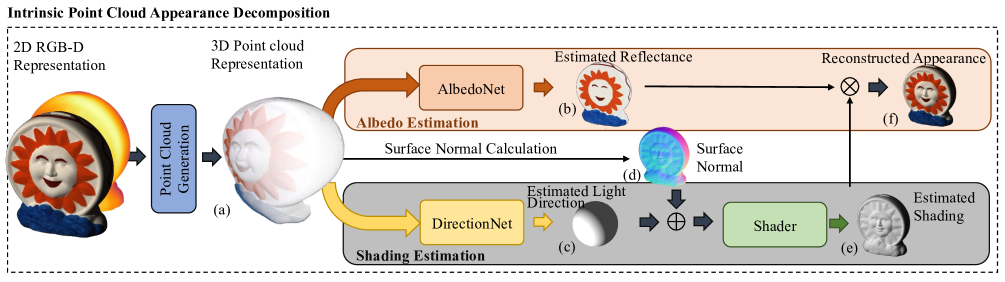
Figure 2: Our proposed framework for intrinsic point cloud decomposition starts by transforming the $RGB-D$ representation to a point cloud representation. (a). The point cloud representation is used as input to train two separate components: the shading and the albedo estimation. The shading estimation is supported by the DirectionNet (Light Direction Estimation Net), which takes (a) as input and and outputs surface light direction estimates (c). Surface normals (d) are calculated using local neighborhoods within (a). The Shader (Learnable Shader) then uses the concatenated vectors of (c) and (d) to generate the final shading estimation (e). The albedo estimation is obtained by the AlbedoNet (Point-Albedo Net) which extracts invariant reflectance (b) from (a) based on the Lambertian assumption. Finally, by multiplying (b) and (e), the reconstructed image (f) is generated. Please refer to the supplementary for the detailed architecture.

3.1 Intrinsic Decomposition

At the surface of a given point $x$, the total reflected radiance $L$ is defined by [14]:

$$L(x,\omega_{o})=\int_{\omega_{i}\in\Omega+}f_{r}(x,\omega_{i},\omega_{o})L_{i}(x,\omega_{i})(N\cdot\omega_{i})d\omega_{i},$$ (1)

where $\omega_{i}$ is the lighting angle from the upper hemisphere $\Omega_{+}$, $\omega_{o}$ is the viewing angle, $N$ is the surface normal, $L_{i}(x,\omega_{i})$ is the position of the lighting angle and its direction, and $f_{r}$ is the surface reflectance, modeled by a Bidirectional Reflectance Distribution Function (BRDF) [26].

Given a viewing angle, if the surface is Lambertian, the diffuse appearance $I_{diffuse}$ formulation is simplified by:

$$\textbf{I}_{diffuse}=\int_{\omega_{i}\in\Omega+}f_{r}(\omega_{i})L_{i}(\omega_{i})(N\cdot\omega_{i})d\omega_{i}.$$ (2)

Conventionally, $\frac{\rho_{d}}{\pi}$ denotes the reflectivity of the surface (albedo), where $f_{r}(\omega_{i})=\frac{\rho_{d}}{2\pi}$. Therefore, if the illumination is uniform, the intrinsic model is defined by:

$$\textbf{I}_{diffuse}=\frac{\rho_{d}}{\pi}\cdot(\textbf{N}\cdot\textbf{L}_{in}),$$ (3)

where, $\textbf{L}_{in}$ represents the visible incident light. The aim of intrinsic decomposition is to disentangle the albedo $\textbf{A}=\frac{\rho_{d}}{\pi}$ and shading $\textbf{S}=(N\cdot L_{in})$ from the appearance $\textbf{I}_{diffuse}$, where $(\cdot)$ is the dot product.

3.2 Intrinsic Appearance on Point Cloud

According to Equation 2, the appearance of the object under a given lighting condition is acquired as a $RGB$ image $\textbf{I}=[\textbf{I}_{r},\textbf{I}_{g},\textbf{I}_{b}]\in\mathbb{R}^{U\times{V}\times 3}$. Additionally, its corresponding depth map is represented by $\mathrm{D}\in\mathbb{R}^{U\times{V}\times 1}$. The depth information can either be directly obtained by a depth camera, e.g., LiDAR, or can be estimated by a (monocular) depth estimation method based on 2D images, e.g.,[30].

Now, the $RGB$ image and corresponding depth map are transformed into a (colored) point cloud representation, $\textbf{P}=\{\textbf{p}_{i}|i\in 1,\ldots,n\}$. Specifically, each point $\textbf{p}_{i}$ is represented as a vector of $[x,y,d,r,g,b]$ values:

$$\textbf{p}_{i}=\left(\frac{(u-c_{x})d}{f_{x}},\frac{(v-c_{y})d}{f_{y}},d,r,g,b\right),$$ (4)

where, $f_{x}$ and $f_{y}$ are the focal lengths, and $(c_{x},c_{y})$ is the principal point.

Given a dataset of $M$ point clouds, $\mathcal{P}=\{\textbf{P}_{1},\textbf{P}_{2},...,\textbf{P}_{M}\}$, its intrinsic components can be defined by: 1) Albedo $\mathcal{A}=\{\textbf{A}_{1},\textbf{A}_{2},...,\textbf{A}_{M}\}$, 2) Shading $\mathcal{S}=\{\textbf{S}_{1},\textbf{S}_{2},...,\textbf{S}_{M}\}$, 3) Surface Normal $\mathcal{N}=\{\textbf{N}_{1},\textbf{N}_{2},...,\textbf{N}_{M}\}$, and 4) Light source position $\mathcal{L}=\{\textbf{L}_{1},\textbf{L}_{2},...,\textbf{L}_{M}\}$.

Albedo contains the invariant (albedo) information. Therefore, a direct point based mapping ($f_{\alpha}:\mathcal{P}\to\mathcal{A}$) is employed to decompose the reflectance appearance from input point cloud.

Shading depends on the object geometry, viewing and lighting conditions. Thus, instead of directly learning the shading, a point-light direction net ($f_{\theta}:\mathcal{P}\to\mathcal{L}$) is used to estimate the light direction from the point cloud representation. Then, a point-learnable shader ($f_{\sigma}:\mathcal{L},\mathcal{N}\to\mathcal{S}$) is trained to generate the rendering effects based on the surface normals (from input point cloud) and light direction estimation (from point-light direction net).

A point cloud representation is beneficial for the intrinsic decomposition task because: 1) point clouds explicitly align depth and $RGB$ information. They are already integrated into one cohesive representation. 2) point clouds provide access to surface normal information. Surface normals can be calculated by local neighborhoods. 3) point clouds provide a robust representation resistant to depth measurement errors. Inaccuracies of a few points will not influence the overall representation.

4 Point Based Intrinsic Decomposition

In this section, a novel point based intrinsic decomposition technique is proposed. Sec. 4.1 provides the technical details of the network architecture; and Sec. 4.2 introduces the learning strategy to train the network.

4.1 Point Intrinsic Net

The proposed point intrinsic network (PoInt-Net) consists of three modules: 1) the Point Albedo-Net, which is designed to learn the material properties of object surfaces, 2) the Light Direction Estimation Net, dedicated to infer the lighting conditions. The aim is to support the estimation of the (point cloud) albedo, and 3) the Learnable shader, which combines the inferred light direction and surface normals to generate the shading map. The closest approach to ours is [13]. However, this method estimates the normal information directly from the input images and can only generalized on single object level.

Figure 2 shows the proposed network architecture and the details of the forward connections. Each of the three sub-nets shares a similar design, with only a few differences such as the activation functions. Specifically, all three sub-nets are adopted from [28], and employ Multi-Layer Perceptrons (MLPs) for point-feature extraction and decoding, with the aim of solving the point-to-point relationship.

Point Albedo-Net takes as input a 6-D point cloud containing color information and spatial coordinates, and produces estimates of surface reflectances. To produce scaled output colors, the Rectified Linear Unit (ReLU) is utilized as the activation function.

Light Direction Estimation Net takes the same input as the Point Albedo-Net, and predicts the point-wise surface light directions. ReLU is used as the activation function in most of the layers. The final two layers use the hyperbolic tangent function (Tanh) to ensure that all light directions are estimated.

Surface Normal Calculation computes the surface normal based on the input point cloud including: 1) neighboring point identification and covariance matrix calculation, 2) eigenvector computation of the covariance matrix, and 3) normal vector selection based on the smallest eigenvalue. To speed up the training process, normal information is pre-computed and used during training.

Learnable Shader takes as input the concatenated vectors of the surface normal information (calculated from the input point cloud) and surface light direction estimation, and outputs the point-wise shading map.

4.2 Joint-learning Strategy

A two-step training strategy is employed to arrive at an end-to-end intrinsic decomposition learning pipeline. First, in terms of shading estimation, the Light Direction Estimation Net and Learnable Shader are trained using ground-truth light position L and shading S. Then, for albedo estimation, the parameters in these two sub-nets are preserved and frozen, while the Point Albedo-Net is constrained by the ground-truth albedo A and the final reconstructed image $\hat{\textbf{I}}$ (multiplied by the estimated albedo map $\hat{\textbf{A}}$ and the estimated shading map $\hat{\textbf{S}}$). During training, the mean square error is used. The loss function, for stage one, is:

$$\mathcal{L}_{shading}=\frac{1}{M}\sum^{M}({|\textbf{L}-\hat{\textbf{L}}|^{2}+|\textbf{S}-\hat{\textbf{S}}|^{2}}).$$ (5)

For stage two, a series of loss functions are used to constrain the invariant color information. To address reflectance changes, a color cross ratio loss inspired by [11] is used, formulated as follows:

$$\mathcal{L}_{ccr}=|M_{RG}-M_{\hat{R}\hat{G}}|+|M_{RB}-M_{\hat{R}\hat{B}}|+|M_{GB}-M_{\hat{G}\hat{B}}|,$$ (6)

where $\{M_{RG},M_{RB},M_{GB}\}$, $\{M_{\hat{R}\hat{G}},M_{\hat{R}\hat{B}},M_{\hat{G}\hat{B}}\}$ are the cross color ratios from the ground-truth albedo and the estimated albedo respectively. Please refer to supplemental for the details of cross color ratios calculation. Similarly to [9], the gradient difference is considered and is formulated by:

$$\mathcal{L}_{grad}=|\nabla\textbf{A}-\nabla\hat{\textbf{A}}|^{2}_{2}$$ (7)

Hence, the reconstruction loss is applied to constrain the estimated albedo:

$$\mathcal{L}_{rec}=\frac{1}{M}\sum^{M}({|\textbf{A}-\hat{\textbf{A}}|^{2}+|\textbf{I}-\hat{\textbf{I}}|^{2}}),$$ (8)

The final loss function is:

$$\mathcal{L}_{albedo}=\mathcal{L}_{rec}+\mathcal{L}_{grad}+\mathcal{L}_{ccr},$$ (9)

where $\{\hat{\cdot}\}$ represents the estimated values, and $M$ is the number of input point clouds in a mini-batch. Adam [16] is employed as the optimizer.

5 Experiments

A number of experiments are conducted to assess the performance of the proposed method in terms of intrinsic decomposition (from single objects to complex scenes), light position estimation and editing (from synthetic to real-world data), and generalization capabilities (from different shapes to different domains). In each subsection, the experiments are categorized based on the objects and scenes which are included in the datasets.

Training Details.

For single object datasets, the point cloud is sampled by voxel downsampling where the voxel size is set to 0.03. For scene datasets, the point cloud is resized to $64\times 64$ points by average downsampling. The batch size is set based on the GPU memory accordingly. Adam [16] is employed as the optimizer. The learning rate is $3\times 10^{-4}$. All networks are trained till convergences.

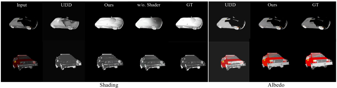
Figure 3: Comparison with state-of-the-art method USI3D [21] and ablation study on the ShapeNet-intrinsic dataset.

5.1 Dataset

Object-level and Scene-level intrinsic image decomposition experiments are conducted on three publicly available datasets:

• ShapeNet-Intrinsic [13]: Based on the ShapeNet [5], albedo and shading are generated by the Blender-cycle. The dataset contains ground-truth depth, normal, and light position information. We follow the same dataset split proposed by Liu et al. [21], using 8979 images for training and 2245 images for evaluation.

• MIT-Intrinsic [12]: Real-world dataset, albedo and shading under different illumination are provided. Depth information, calculated by [1], is used. The train and test split are kept the same as proposed by [1].

• MPI-Sintel [4]: is a synthetic dataset and provides albedo, shading, and depth information. The same training and test splits are used compared to existing methods to evaluate our method.

In addition, we employ multiple images downloaded from internet to demonstrate our generalization ability for the real-word scenarios.

5.2 Intrinsic Decomposition: Single Objects

We first train PoInt-Net on the ShapeNet dataset, with ground-truth labels for intrinsic images and light positions. Then, the pre-trained parameters are fine-tuned on the MIT-intrinsic dataset, with only ground truth labels for intrinsic images. This corresponds to a self-supervised learning problem for light position estimation.

The quantitative and qualitative results are presented. For the numerical results, three common metrics are employed for evaluation: mean square error (MSE), local mean squared error (LMSE), and structural dissimilarity (DSSIM).

ShapeNet-Intrinsic

	MSE$\times 10^{2}$			LMSE$\times 10^{2}$	DSSIM$\times 10^{2}$
	A	S	Avg.	Total	Total
CGIntrinsics[20]	3.38	2.96	3.17	6.23	-
Fan et al. [9]	3.02	3.15	3.09	7.17	-
Ma et al. [23]	2.84	2.62	2.73	5.44	-
USI3D [21]	1.85	1.08	1.47	4.65	-
Ours (w/o. shader)	0.48	0.57	0.53	1.15	4.93
Ours	0.46	0.38	0.42	1.00	4.15

Table 1: Numerical comparison and ablation study on ShapeNet intrinsic dataset. The top-3 results on each column are highlighted by red yellow and gray, respectively.

Table 1 shows a quantitative comparison of PoInt-Net with state-of-the-art techniques on the ShapeNet intrinsic dataset. We compare our approach to the latest open source methods [20, 23, 9, 21]. The results demonstrate that our approach outperforms existing methods by a large margin for all three metrics. Specifically, PoInt-Net achieves a MSE of 0.0046 in albedo and 0.0038 in shading, LMSE 1.00 in total, and DSSIM 0.0415 in total. These results show the effectiveness of our approach in accurately predicting the intrinsic properties. The high performance of our method can be attributed to its ability to capture and leverage the complex relationships among the intrinsic properties, resulting in a more robust and reliable estimation.

The qualitative results of the method are presented in Figure 3, where USI3D [21] (fine-tuned version) is used as a reference. PoInt-Net outputs a shading map based on the surface light direction and surface normal, which allows to accurately separate the shading from the composite image. Consequently, the output images display realistic and consistent shading that closely reflects the underlying surface geometry. Decomposing shading from the composited image is evident in the darker areas of the objects, where a more distinct separation between the shading and the object surface can be observed. These results show the effectiveness and robustness of the method in producing high-quality and visually appealing outputs that accurately capture the intrinsic properties of the objects.

	MSE$\times 10^{2}$		LMSE$\times 10^{2}$		DSSIM$\times 10^{2}$
	A	S	A	S	A	S
SIRFS [1]	1.47	0.83	4.16	1.68	12.38	9.85
Zhou et al. [36]	2.52	2.29	-	-	-	-
Shi et al. [32]	2.78	1.26	5.03	2.40	14.65	12.00
DI [25]	2.77	1.54	5.86	2.95	15.26	13.28
CGIntrinsics [20]	1.67	1.27	3.19	2.21	12.87	13.76
Ma et al. [23]	3.13	2.07	1.16	0.95	-	-
Janner et al. [13]	3.36	1.95	2.10	1.03	-	-
USI3D [21]	1.57	1.35	1.46	2.31	-	-
FFI-Net [29]	1.11	0.93	2.91	3.19	10.14	11.39
PIE-Net [8]	0.28	0.35	1.36	1.83	3.40	4.93
Ours	0.89	0.34	0.97	0.37	4.39	3.02

Table 2: Results for MIT Intrinsic. All methods use the training-test split file released by [1]. The color system are same as Table 1.

MIT-intrinsic

In addition to the synthetic dataset, this section provides an evaluation on the MIT-intrinsic dataset to assess the proposed method’s ability to generalize to real-world scenarios. The results obtained on the MIT-intrinsic dataset are consistent with those obtained on the synthetic dataset, demonstrating the effectiveness and robustness of the method across different datasets.

Table 2 reports the quantitative results. PoInt-Net produces state-of-the-art shading results on the MIT-intrinsic dataset for all metrics. Moreover, our approach obtains the best LMSE and the second-best performance for the albedo output in terms of MSE and DSSIM metrics. Note that [8] employs an extra input to provide additional information for albedo estimation.

The visualization results are depicted in Figure 4. Our method outperforms others in the ability to accurately distinguish the spots on the back of the frog. This is because PoInt-Net’s use of surface light direction estimation and surface normal calculation to produce high-quality shading results. Moreover, despite the absence of ground-truth light source position, PoInt-Net’s surface light direction estimation is learned in a self-supervised manner.

Discussion: Ground-truth depth information is not included in the MIT-intrinsic dataset. To this end, depth information is used computed by Barron et al. [1]. However, these depth estimations are noisy containing outliers and invalid points. Nevertheless, PoInt-Net consistently learns intrinsic features even when the input contains noise, demonstrating its robustness to imperfect depth information.

5.3 Intrinsic Decomposition: Complex Scenes

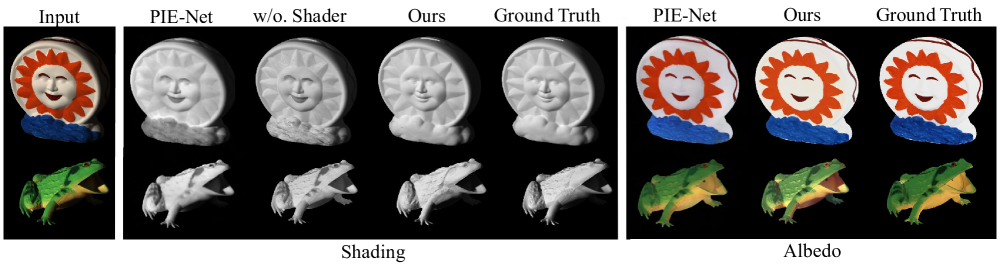
Figure 4: Qualitative results on the MIT-intrinsic benchmark [12]. Comparison to the state-of-the-art method PIE-Net [8]. Ablation study on shader is conducted.

Sintel	si-MSE$\times 10^{2}$			si-LMSE$\times 10^{2}$			DSSIM$\times 10^{2}$
	A	S	avg	A	S	avg	A	S	avg
Retinex [12]	6.06	7.27	6.67	3.66	4.19	3.93	22.70	24.00	23.35
Lee et al. [18]	4.63	5.07	4.85	2.24	1.92	2.08	19.90	17.70	18.80
SIRFS  [1]	4.20	4.36	4.28	2.98	2.64	2.81	21.00	20.60	20.80
Chen et al. [6]	3.07	2.77	2.92	1.85	1.90	1.88	19.60	16.50	18.05
DI [25]	1.00	0.92	0.96	0.83	0.85	0.84	20.14	15.05	17.60
DARN [19]	1.24	1.28	1.26	0.69	0.70	0.70	12.63	12.13	12.38
Kim et al. [15]	0.70	0.90	0.70	0.60	0.70	0.70	9.20	10.10	9.70
Fan et al. [9]	0.69	0.59	0.64	0.44	0.42	0.43	11.94	8.22	10.08
LapPyrNet [7]	0.66	0.60	0.63	0.44	0.42	0.43	6.56	6.37	6.47
USI3D [21]	1.59	1.48	1.54	0.87	0.81	0.84	17.97	14.74	16.35
Ours	0.57	0.71	0.64	0.29	0.38	0.34	8.74	8.83	8.79

Table 3: Numerical results for MPI-Sintel (image split), the color is same as Table 1.

.

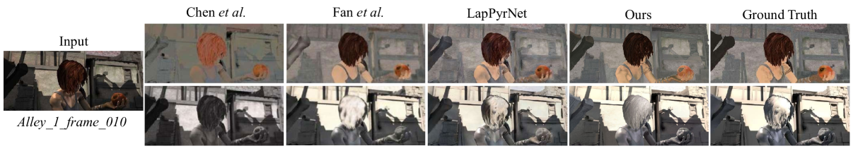
Figure 5: Visual results (image split) on the MPI Sintel dataset [4]. Comparison to state-of-art-methods Fan et al. [9] and LapPrNet[7]. The method of Chen et al. [6] is provided as reference, since it uses $RGB-D$ images as input.

The MPI-Sintel dataset differs from object-wise datasets, since it has color for each pixel. For a fair evaluation, we follow the approach in [9] by using scale invariant MSE (si-MSE) and local scale invariant MSE (si-LMSE).

It can be derived from the quantitative results, presented in Table 3, that PoInt-Net can be applied to complex scenes. We compare our approach to several state-of-the-art methods, whose results are reported either in the original paper or through re-implementation. Our approach outperforms state-of-the-art methods in terms of si-LMSE for albedo and shading, as well as si-MSE for albedo. Additionally, PoInt-Net provides competitive performance for si-MSE shading and ranks second-best on DSSIM, demonstrating its ability to deal with complex scenes with varying lighting conditions. Qualitative results are shown in Figure 5, where PoInt-Net produces high-quality results, especially in the sharpness. This is beneficial for the point-based intrinsic net, where the intrinsic features are processed point-by-point. Compared to [6], also using depth information for intrinsic decomposition, PoInt-Net shows to have a consistently better reflectance and shading estimation. This is mainly due to the use of a point cloud representation. Please refer to the supplemental material for additional results.

5.4 Free Light Position Relighting

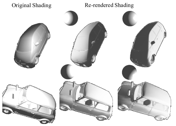
Figure 6: Relighting results on the Shape-Net intrinsic dataset. The grey sphere corresponds to the light direction.

The proposed shader method of the point-intrinsic network is able to generate shading for different light positions. The predicted surface light direction is replaced by a new surface light direction under a given light position, then concatenated with the surface normal and used by the learnable shader to render the new shading.

Since there is no ground truth for relighting, quantitative results can not be computed. Hence, we use the grey sphere to indicate the given light position according to [13].

ShapeNet-Intrinsic

The qualitative results of the proposed learnable shader are presented in Figure 6. It is shown that the learnable shader is capable of generating new shading based on the given light position. The approach’s ability to learn and adapt to different lighting conditions is demonstrated by the consistent and accurate shading of the objects across different light positions. The shading is not only realistic but also visually appealing, exhibiting a high level of detail and accuracy. These results show the effectiveness of the proposed approach in generating high-quality and customizable shading that can adapt to varying lighting conditions.

Discussion: In contrast to the light transfer approach described in [13], which involves rendering a single object multiple times with different light source positions to train the shader, PoInt-Net uses each object with the same viewing angle only once during training. Despite of using less data, our results demonstrate that our learnable shader is efficient and robust. It is able to accurately distinguish the relationship between surface light direction and shading.

5.5 Generalization to Unseen Objects/Scenes

To evaluate the generalization capability of our method, we conduct real-world decompositions. It consists of three steps: 1) 2D images are downloaded from the internet; 2) a monocular depth estimation method is employed to calculate the depth map; 3) the pre-trained model is used to generate the intrinsics for these unseen objects/scenes.

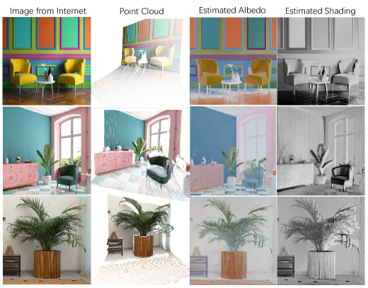
Figure 7: Real-world intrinsic estimated by PoInt-Net. Although the model is only trained on single object level datasets, our approach provides proper intrinsic computation for unseen objects/scenes. Images are taken from the Internet. Zoom to see details.

Figure 7 shows the robust generalization of PoInt-Net on real-world images, where images are randomly downloaded from internet. The point clouds are generated based on the estimated depth maps from [30], accordingly. Although, PoInt-Net is trained on the single object level dataset (details in Sec. 5.2). It can still accurately estimate the surface reflectance and shading, for single objects and complex scenes, e.g., the shadow region between the sofa and the wall. Please refer to supplemental for more details and results.

5.6 Ablation Study

Learnable shader.

As illustrated in Sec 3.2, shading depends on the surface geometry. Table 1 shows that the shader plays an important role increasing the shading quality numerically. Figure 3 and Figure 4 show that the shader supports PoInt-Net to differentiate between invariant and ambient colors. Such as the face and cloud parts of ”Sun” from MIT-Intrinsic, which used to be a terribly challenge for most of learning methods. (More comparison please refer to Supplemental.)

Model size of networks.

As presented in Figure 8, our method shows superior performance for intrinsics estimation, while having a small model size. The model size is reported based on its official per-trained model accordingly. In general, our method keeps a smaller model than others, which use an extra mapping module [21], adversarial network [37], multi-scale CNN [7], and transformer [8] in their network architecture.

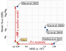
Figure 8: Model size (MB) vs. MSE ($\times 10^{2}$) on shading for the MIT-intrinsic dataset. Our method is highly efficient, outperforming the state-of-the-art model with just 1/100 of the model size and achieving 5 times the accuracy of a model with a similar size.

6 Conclusion

We proposed point intrinsic representation and point intrinsic network (PoInt-Net) to achieve 3D represented intrinsic decomposition. Different from existing methods, PoInt-Net employs a point cloud representation to address the intrinsic decomposition problem, leverages the unique properties of point clouds to effectively decompose surface light direction, surface reflectance, and shading maps. Our method is both simple and efficient, requiring only 1/100 of the model size of state-of-the-art methods while outperforming them in surface shading estimation on the MIT-intrinsic dataset. Experiments for different shapes/scenes and across domains demonstrate the robustness and efficiency of our approach. We believe that our method not only offers a new solution for intrinsic decomposition, but also opens up a promising research direction to use point cloud representations in low-level vision tasks such as color constancy and material recognition.

Limitations.

Our method is based on Lambertain assumption, also, the surface light direction prediction is only trained on single light source scenarios. We argue that, in the future, non-Lambertain and multiple-light source scenarios need to be addressed.

Appendix A Details of Point Cloud Generation

Acquiring Depth Map.

As introduced in Section 3.2, a corresponding depth map $D$ is needed to generate a point cloud from a 2D image. For some datasets, e.g., ShapeNet-Intrinsic and MPI-Sintel. They provide the ground truth depth information, since they are synthetic dataset. For the real world dataset like MIT-Intrinsic, Barron et al. [1] calculates the depth information. Except that, the depth information can be easily estimated by a monocular depth estimation method, such as [30].

Camera Intrinsic Matrix.

In Equation 4, the camera intrinsic matrix is employed to translate the point cloud from RGB-D image, i.e., images $\textbf{I}=[\textbf{I}_{r},\textbf{I}_{g},\textbf{I}_{b}]\in\mathbb{R}^{U\times{V}\times 3}$ and depth map $\mathrm{D}\in\mathbb{R}^{U\times{V}\times 1}$. For the MPI-Sintel dataset, we use the intrinsic matrix provide from the dataset. For other datasets, we use a default setting for the intrinsic matrix, where as the focal lengths and principal point are set as $(\frac{1}{2}{U},\frac{1}{2}{V})$, respectively.

Appendix B Point Intrinsic Net: Architecture

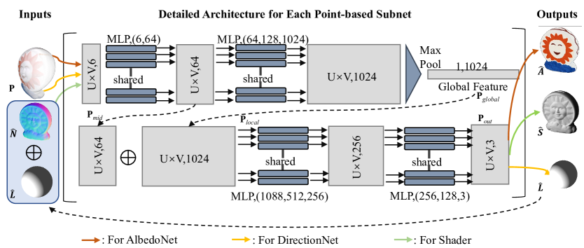
Figure 9: The detailed architecture of the sub-net of point intrinsic network (PoInt-Net), which is a slightly modified version of PointNet [28]. For the internal connection of each subnet please refer to Figure 2 in the main paper. The three colors represent the in/out put, for three different subnets, respectively.

Figure 9 demonstrates the detailed architecture of the subnet of PoInt-Net. The input feature $\textbf{P}_{input}\in\mathbb{R}^{U\times{V}\times 6}$ is first extracted by MLPs, and Max Pooling is employed to extract the significant global feature $\textbf{P}_{global}\in\mathbb{R}^{1\times 1024}$. To maintain the ability in solving local information, the global feature is then repeated to the same number as the input points, and then concatenate with the inter-midden feature $\textbf{P}_{mid}\in\mathbb{R}^{U\times{V}\times{64}}$ to get the local feature $\textbf{P}_{local}\in\mathbb{R}^{U\times{V}\times 1088}$. Finally, the output $\textbf{P}_{output}\in\mathbb{R}^{U\times{V}\times 3}$ is obtained by MLPs which act as channel wise decoder. Since the three subnets share the similar network architecture, we use different color of the arrow to indicate the different input for the different nets, the color refer to the same color used in the Figure 2 of the main paper.

Appendix C Cross Color Ratios Loss Calculation

In paper, we propose the cross color ratios (CCR) loss to address the reflectance changes. Where the CCR $\{M_{RG},M_{RB},M_{GB}\}$ is calculated as:

$$M_{RG}=\frac{R_{p1}G_{p2}}{R_{p2}G_{p1}},M_{RB}=\frac{R_{p1}B_{p2}}{R_{p2}B_{p1}},M_{GB}=\frac{G_{p1}B_{p2}}{G_{p2}B_{p1}},$$ (10)

where the $\{R_{p1},G_{p1},B_{p1}\}$ and $\{R_{p2},G_{p2},B_{p2}\}$ represent the $R,G,B$ value at the two adjacent points $p_{1}$ and $p_{2}$, respectively.

Appendix D Implementation Details

Building Point Cloud.

We generate the point cloud based on a pair of RGB image and its corresponding depth information. Normal information is pre-computed from the point cloud, which can be performed online or in advance for faster training and inference.

Calculating Depth.

In the absence of depth information, we utilize the open-source monocular depth estimation method, MiDaS [30], to estimate depth from the image. While any monocular depth estimation method can technically be used, we choose MiDaS due to its stability and ease of implementation.

Environment Setting.

PoInt-Net is developed using the PyTorch framework, enabling it to run on both CPU and GPU platforms. During evaluation, our method runs on a single NVIDIA 1080Ti GPU, with inference times dependent on the image size. For a 512$\times$512 image, the average inference time is $\sim$ 10 frames per second. It’s important to note that this inference time is achieved without any pruning techniques applied.

Appendix E More Results: Intrinsic Decomposition

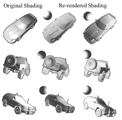
Figure 10: Visual results for free-light position relighting. The gray sphere only indicates the light source direction.

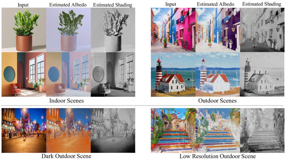
Figure 11: Visualization results across different shapes, scenes, and domains in the real world. Our method consistently estimates the reasonable results. Note: our method is only trained on single-object level datasets.

Real World.

The monocular depth estimation technique used in PoInt-Net enables it to decompose intrinsic properties in real-world scenarios. In Figure 11, we present additional visualization results from various scenes, including indoor and outdoor environments. PoInt-Net produces reliable results for both reflectance and shading estimation. Remarkably, even in challenging scenarios, such as dark or low-resolution outdoor scenes, PoInt-Net is capable of decomposing invariant colors and estimating accurate shading.

As discussed in the paper, PoInt-Net is trained on single-object level datasets, i.e., ShapeNet-Intrinsic and MIT-Intrinsic. However, our method still achieves impressive intrinsic decomposition results across various shapes, scenes, and domains. These findings suggest that PoInt-Net is capable of solving intrinsic decomposition tasks at a very low-level, highlighting its robustness and versatility.

ShapeNet-Intrinsic.

We present additional results on the ShapeNet dataset in Figure 12. These results showcase PoInt-Net’s ability to estimate surface light direction, with direct shading results displayed in the second column of the figure.

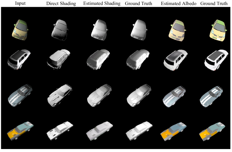
Figure 12: Qualitative results on ShapeNet-Intrinsic dataset. The Direct shading is computed by surface normal and surface light direction.

MIT-Intrinsic.

Figure 13 presents additional results on the MIT-Intrinsic dataset, including ablation study results for the shader. The findings demonstrate that the shader significantly enhances PoInt-Net’s ability to distinguish between invariant color and illumination.

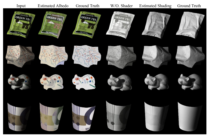
Figure 13: Qualitative results on MIT-Intrinsic dataset. The ablation study on the shader (W/O. Shader) is applied.

MPI-Sintel.

Figure 14 presents extensional results that provide evidence for PoInt-Net’s ability to handle complex scenes during intrinsic decomposition training. The findings suggest that the architecture of PoInt-Net is capable of undertaking such tasks effectively.

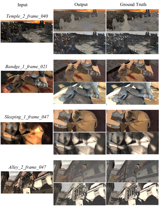
Figure 14: Visual results on MPI-Sintel dataset.

Appendix F More Results: Relighting

Figure 10 showcases additional qualitative results for free light-position relighting. In the figure, a gray sphere is utilized to indicate the given light position. Notably, PoInt-Net is trained without the use of any extra lighting images, yet it still successfully learns the pattern for relighting. These findings provide further evidence of the efficiency and robustness of our model design.

Appendix G Discussion: Depth Quality

Depth information plays a critical role in our method, particularly in shading estimation. As demonstrated in Figure 7 and Figure 11, real-world image shading often contains artifacts that result from the calculated depth maps generated by [30], which are prone to discontinuities and flickering.

More figures are presented in next pages.

References

- [1] Jonathan T Barron and Jitendra Malik. Shape, illumination, and reflectance from shading. IEEE TPAMI, 37(8):1670–1687, 2015.
- [2] Anil S Baslamisli, Partha Das, Hoang-An Le, Sezer Karaoglu, and Theo Gevers. Shadingnet: Image intrinsics by fine-grained shading decomposition. IJCV, 129(8):2445–2473, 2021.
- [3] Anil S Baslamisli, Hoang-An Le, and Theo Gevers. Cnn based learning using reflection and retinex models for intrinsic image decomposition. In CVPR, 2018.
- [4] Daniel J Butler, Jonas Wulff, Garrett B Stanley, and Michael J Black. A naturalistic open source movie for optical flow evaluation. In ECCV, 2012.
- [5] Angel X. Chang, Thomas Funkhouser, Leonidas Guibas, Pat Hanrahan, Qixing Huang, Zimo Li, Silvio Savarese, Manolis Savva, Shuran Song, Hao Su, Jianxiong Xiao, Li Yi, and Fisher Yu. ShapeNet: An Information-Rich 3D Model Repository. Technical Report arXiv:1512.03012 [cs.GR], Stanford University — Princeton University — Toyota Technological Institute at Chicago, 2015.
- [6] Qifeng Chen and Vladlen Koltun. A simple model for intrinsic image decomposition with depth cues. In ICCV, 2013.
- [7] Lechao Cheng, Chengyi Zhang, and Zicheng Liao. Intrinsic image transformation via scale space decomposition. In CVPR, 2018.
- [8] Partha Das, Sezer Karaoglu, and Theo Gevers. Pie-net: Photometric invariant edge guided network for intrinsic image decomposition. In CVPR, 2022.
- [9] Qingnan Fan, Jiaolong Yang, Gang Hua, Baoquan Chen, and David Wipf. Revisiting deep intrinsic image decompositions. In CVPR, 2018.
- [10] David Forsyth and Jason J Rock. Intrinsic image decomposition using paradigms. IEEE TPAMI, 44(11):7624–7637, 2021.
- [11] Theo Gevers and Arnold WM Smeulders. Color-based object recognition. Pattern recognition, 32(3):453–464, 1999.
- [12] Roger Grosse, Micah K Johnson, Edward H Adelson, and William T Freeman. Ground truth dataset and baseline evaluations for intrinsic image algorithms. In ICCV, 2009.
- [13] Michael Janner, Jiajun Wu, Tejas D Kulkarni, Ilker Yildirim, and Josh Tenenbaum. Self-supervised intrinsic image decomposition. In NIPS, 2017.
- [14] James T Kajiya. The rendering equation. In SIGGRAPH, pages 143–150, 1986.
- [15] Seungryong Kim, Kihong Park, Kwanghoon Sohn, and Stephen Lin. Unified depth prediction and intrinsic image decomposition from a single image via joint convolutional neural fields. In ECCV, 2016.
- [16] Diederik P Kingma and Jimmy Ba. Adam: A method for stochastic optimization. arXiv preprint arXiv:1412.6980, 2014.
- [17] Pierre-Yves Laffont and Jean-Charles Bazin. Intrinsic decomposition of image sequences from local temporal variations. In ICCV, pages 433–441, 2015.
- [18] Kyong Joon Lee, Qi Zhao, Xin Tong, Minmin Gong, Shahram Izadi, Sang Uk Lee, Ping Tan, and Stephen Lin. Estimation of intrinsic image sequences from image+ depth video. In ECCV, 2012.
- [19] Louis Lettry, Kenneth Vanhoey, and Luc Van Gool. Darn: a deep adversarial residual network for intrinsic image decomposition. In WACV, 2018.
- [20] Zhengqi Li and Noah Snavely. Learning intrinsic image decomposition from watching the world. CVPR, 2018.
- [21] Yunfei Liu, Yu Li, Shaodi You, and Feng Lu. Unsupervised learning for intrinsic image decomposition from a single image. In CVPR, 2020.
- [22] Jundan Luo, Zhaoyang Huang, Yijin Li, Xiaowei Zhou, Guofeng Zhang, and Hujun Bao. Niid-net: adapting surface normal knowledge for intrinsic image decomposition in indoor scenes. IEEE TVCG, 26(12):3434–3445, 2020.
- [23] Wei-Chiu Ma, Hang Chu, Bolei Zhou, Raquel Urtasun, and Antonio Torralba. Single image intrinsic decomposition without a single intrinsic image. In ECCV, 2018.
- [24] Ben Mildenhall, Pratul P Srinivasan, Matthew Tancik, Jonathan T Barron, Ravi Ramamoorthi, and Ren Ng. Nerf: Representing scenes as neural radiance fields for view synthesis. In ECCV, pages 405–421. Springer, 2020.
- [25] Takuya Narihira, Michael Maire, and Stella X Yu. Direct intrinsics: Learning albedo-shading decomposition by convolutional regression. In ICCV, 2015.
- [26] Fred E Nicodemus. Directional reflectance and emissivity of an opaque surface. Applied optics, 4(7):767–775, 1965.
- [27] Julian Ost, Issam Laradji, Alejandro Newell, Yuval Bahat, and Felix Heide. Neural point light fields. In CVPR, pages 18419–18429, 2022.
- [28] Charles R Qi, Hao Su, Kaichun Mo, and Leonidas J Guibas. Pointnet: Deep learning on point sets for 3d classification and segmentation. In CVPR, pages 652–660, 2017.
- [29] Yanlin Qian, Miaojing Shi, Joni-Kristian Kamarainen, and Jiri Matas. Fast fourier intrinsic network. In WACV, 2021.
- [30] René Ranftl, Katrin Lasinger, David Hafner, Konrad Schindler, and Vladlen Koltun. Towards robust monocular depth estimation: Mixing datasets for zero-shot cross-dataset transfer. IEEE TPAMI, 44(3), 2022.
- [31] Li Shen, Chuohao Yeo, and Binh-Son Hua. Intrinsic image decomposition using a sparse representation of reflectance. IEEE TPAMI, 35(12):2904–2915, 2013.
- [32] Jian Shi, Yue Dong, Hao Su, and X Yu Stella. Learning non-lambertian object intrinsics across shapenet categories. In CVPR, 2017.
- [33] Xiaoyan Xing, Yanlin Qian, Sibo Feng, Yuhan Dong, and Jiří Matas. Point cloud color constancy. In CVPR, 2022.
- [34] Qiangeng Xu, Zexiang Xu, Julien Philip, Sai Bi, Zhixin Shu, Kalyan Sunkavalli, and Ulrich Neumann. Point-nerf: Point-based neural radiance fields. In CVPR, 2022.
- [35] Xiuming Zhang, Pratul P Srinivasan, Boyang Deng, Paul Debevec, William T Freeman, and Jonathan T Barron. Nerfactor: Neural factorization of shape and reflectance under an unknown illumination. ACM TOG, 40(6):1–18, 2021.
- [36] Tinghui Zhou, Philipp Krahenbuhl, and Alexei A Efros. Learning data-driven reflectance priors for intrinsic image decomposition. In CVPR, 2015.
- [37] Daniel Zoran, Phillip Isola, Dilip Krishnan, and William T Freeman. Learning ordinal relationships for mid-level vision. In CVPR, 2015.