A Parametric Study of the SASI Comparing General Relativistic and Non-Relativistic Treatments

Abstract

We present numerical results from a parameter study of the standing accretion shock instability (SASI), investigating the impact of general relativity (GR) on the dynamics. Using GR hydrodynamics and gravity, and non-relativistic (NR) hydrodynamics and gravity, in an idealized model setting, we vary the initial radius of the shock and, by varying its mass and radius in concert, the proto-neutron star (PNS) compactness. We investigate two regimes expected in a post-bounce core-collapse supernova (CCSN): one meant to resemble a relatively low-compactness configuration and one meant to resemble a relatively high-compactness configuration. We find that GR leads to a longer SASI oscillation period, with ratios between the GR and NR cases as large as 1.29 for the high-compactness suite. We also find that GR leads to a slower SASI growth rate, with ratios between the GR and NR cases as low as 0.47 for the high-compactness suite. We discuss implications of our results for CCSN simulations.

1 Introduction

Since the discovery of the standing accretion shock instability (SASI; Blondin et al., 2003), which many two- and three-dimensional simulations performed to date demonstrate becomes manifest during a core-collapse supernova (CCSN) in the post-shock accretion flow onto the proto-neutron star (PNS), groups have made efforts to understand its physical origin and its effects on the supernova itself. The SASI is characterized in two dimensions (2D) by a large-scale “sloshing” of the shocked fluid, and in three dimensions (3D) by additional spiral modes (Blondin & Mezzacappa, 2007). It is now generally accepted that turbulent neutrino-driven convection plays a major role in re-energizing the stalled shock (e.g., see Burrows et al., 2012; Hanke et al., 2013; Murphy et al., 2013; Couch & Ott, 2015; Melson et al., 2015b; Lentz et al., 2015; Abdikamalov et al., 2015; Radice et al., 2015; Melson et al., 2015b, a; Roberts et al., 2016; Müller et al., 2017; Summa et al., 2018; Radice et al., 2018; O’Connor & Couch, 2018a; Vartanyan et al., 2019; Müller et al., 2019; Burrows et al., 2019; Yoshida et al., 2019; Powell & Müller, 2020; Stockinger et al., 2020; Müller & Varma, 2020; Vartanyan et al., 2022; Nakamura et al., 2022; Matsumoto et al., 2022). The same simulations that led to the above conclusion also generally exhibit the SASI, with outcomes ranging from convection-dominated flows to SASI-dominated flows, and flows where neither dominates. Strong SASI activity and, in some cases, SASI-aided explosions have been reported in, for example, the three-dimensional simulations of Summa et al. (2018), O’Connor & Couch (2018a), and Matsumoto et al. (2022). A more precise determination of the relative role played by these two instabilities in the explosion mechanism, on a case-by-case basis (i.e., for different progenitor characteristics; e.g., see Scheck et al., 2008; Hanke et al., 2012, 2013; Couch & O’Connor, 2014; Fernández et al., 2014; Melson et al., 2015a; Abdikamalov et al., 2015; Fernández, 2015), will require advances in current three-dimensional models to include full general relativity, rotation, magnetic fields, and the requisite neutrino interaction physics with realistic spectral neutrino kinetics, all at high spatial resolution. It is also important to note that, while convection-dominated and SASI-dominated scenarios may lie at the extremes of what is possible, it is not necessary for one or the other instability to be dominant to play an important role – specifically, for the more complex cases where neither dominates, it would be impossible to determine precisely the relative contribution from these two instabilities.

Several studies have concluded that the SASI is an advective-acoustic instability, in which vortical waves generated at the shock advect to the surface of the PNS, which in turn generate acoustic waves that propagate back to the shock and further perturb it (Foglizzo et al., 2006, 2007; Yamasaki & Yamada, 2007; Laming, 2007, 2008; Foglizzo, 2009; Guilet & Foglizzo, 2012). This perturbation generates more vortical waves, which advect to the PNS surface, thus creating a feedback loop that drives the instability. An alternative explanation for the SASI is the purely acoustic mechanism, in which acoustic perturbations just below the shock travel around the post-shock region and constructively interfere with each other, generating stronger acoustic perturbations and thereby feeding the instability (Blondin & Mezzacappa, 2006). A recent study (Walk et al., 2023) suggests that the acoustic mechanism may play a particularly important role in the SASI when rotation is included, implying that the origins of the SASI excitation may depend on conditions between the shock and the PNS.

Other numerical studies focus on particular aspects of this instability, such as the hydrodynamics of the SASI (Ohnishi et al., 2006; Sato et al., 2009; Iwakami et al., 2014), spiral modes (Blondin & Shaw, 2007; Iwakami et al., 2008; Fernández, 2010), the spin-up of the possible remnant pulsar (Blondin & Mezzacappa, 2007), the effect of nuclear dissociation (Fernández & Thompson, 2009), saturation of the instability (Guilet et al., 2010), the generation and amplification of magnetic fields (Endeve et al., 2010, 2012), the relative importance of the SASI and convection in CCSNe (Cardall & Budiardja, 2015), the generation of, and impact on, gravitational waves by the SASI (Kotake et al., 2007, 2009; Kuroda et al., 2016; Andresen, 2017; Kuroda et al., 2017; Andresen et al., 2017; O’Connor & Couch, 2018a; Hayama et al., 2018; Andresen et al., 2019; Mezzacappa et al., 2020, 2023; Drago et al., 2023), and the effects of rotation (Yamasaki & Yamada, 2005; Yamasaki & Foglizzo, 2008; Walk et al., 2023; Buellet et al., 2023). Some of these studies included sophisticated microphysics, such as realistic equations of state (EoSs), and neutrino transport; however, with the exception of Kuroda et al. (2017), none of these studies solved the general relativistic hydrodynamics (GRHD) equations, instead solving their non-relativistic (NRHD) counterparts, some with an approximate relativistic gravitational potential. It has been demonstrated that GR effects are crucial to include in CCSN simulations (Bruenn et al., 2001; Müller et al., 2012; Lentz et al., 2012; O’Connor & Couch, 2018b), yet the SASI itself has not been fully investigated in the GR regime. A recent paper (Kundu & Coughlin, 2022) does analyze steady state accretion through a stationary shock onto compact objects in a Schwarzchild geometry and compares with Newtonian solutions, and posits that GR may have a non-negligible impact on the SASI. They find that, for conditions expected in exploding CCSNe, the freefall speed is of order $v\sim 0.2\,c$ (with $c$ the speed of light), and the differences between the GR and NR solutions are of order 10%. For conditions expected in failed CCSNe (i.e., supernovae where the shock is not revived, in which case the freefall speed can be $v\sim 0.66\,c$), the differences can be larger.

The timescales that likely influence the SASI depend on signal-speeds associated with advective and acoustic modes in the region between the shock and the PNS surface (Blondin & Mezzacappa, 2006; Foglizzo et al., 2007; Müller, 2020). Motivated in part by Dunham et al. (2020) and Kundu & Coughlin (2022), we expect SASI simulations to behave differently depending on whether or not the treatment of the hydrodynamics and gravity are general relativistic. Specifically, we expect both advective and acoustic modes to be influenced by the different post-shock structure in the GR case relative to the NR case.

This leads to our main science question: How does a general relativistic treatment of hydrodynamics and gravity affect the oscillation period and growth rate of the SASI? To begin to address this, we present the first comparison of the SASI in both a non-relativistic and a general relativistic framework, using an idealized model under two sets of conditions: one set is mildly relativistic and is designed to mirror low-compactness conditions after bounce in a CCSN, and the other set is strongly relativistic and is designed to mirror high-compactness conditions. We focus our attention on the linear regime and characterize the SASI by its growth rate and oscillation period, as was done in Blondin & Mezzacappa (2006). To capture both the linear regime of the SASI and its transition to the nonlinear regime, we perform our assessment via two suites of axisymmetric numerical simulations, differentiated by their compactness, using GRHD and GR gravity, with the PNS represented by a point mass and gravity encoded in a Schwarzchild spacetime metric. To better assess the impact of GR, we also perform simulations using the same parameter sets but with NRHD and Newtonian gravity, again with the PNS represented by a point mass, but in this case gravity is encoded in the Newtonian potential.

We use a system of units in which $c=G=1$ and also make use of the Einstein summation convention, with Greek indices running from 0 to 3 and Latin indices running from 1 to 3.

2 Physical Model

2.1 Relativistic Gravity: Conformally-Flat Condition

We use the 3+1 decomposition of spacetime (see, e.g., Banyuls et al., 1997; Gourgoulhon, 2012; Rezzolla & Zanotti, 2013, for details), which, in the coordinate system $x=\left(t,x^{i}\right)$, introduces four degrees of freedom: the lapse function, $\alpha\left(x\right)$, and the three components of the shift vector, $\beta^{i}\left(x\right)$. We further specialize to the conformally-flat condition (CFC, Wilson et al., 1996), effectively neglecting the impact of gravitational waves on the dynamics. This is a valid approximation when the CCSN progenitor is non-rotating (Dimmelmeier et al., 2005), as is the case for our simulations. The CFC forces the components of the spatial three-metric, $\gamma_{ij}\left(x\right)$, to take the form

$$\gamma_{ij}=\psi^{4}\,\overline{\gamma}_{ij},$$ (1)

where $\psi\left(x\right)$ is the conformal factor and the $\overline{\gamma}_{ij}$ are the components of a time-independent, flat-space metric. We choose an isotropic spherical-polar coordinate system, as it is appropriate to our problem and is consistent with the CFC; the flat-space metric is

$$\overline{\gamma}_{ij}\left(r,\theta\right):=\mathrm{diag}\left(1,r^{2},r^{2}\,\sin^{2}\theta\right),$$ (2)

and the lapse function, conformal factor, and shift vector take the form given in Baumgarte & Shapiro (2010),

$$\alpha\left(t,r,\theta,\varphi\right) =\alpha\left(r\right) :=\frac{1-r_{s}/r}{1+r_{s}/r},$$ (3)

$$\psi\left(t,r,\theta,\varphi\right) =\psi\left(r\right) :=1+r_{s}/r,$$ (4)

$$\beta^{i}\left(t,r,\theta,\varphi\right) =\beta^{i}\left(r\right) :=0,$$ (5)

where $r>r_{s}$ is the isotropic radial coordinate measured from the origin and $r_{s}:=M/2$ is the Schwarzchild radius in isotropic coordinates for an object of mass $M$. The line element under a 3+1 decomposition in isotropic coordinates takes the form

$$ds^{2}=-\alpha^{2}\,dt^{2}+\gamma_{ij}\,dx^{i}\,dx^{j}.$$ (6)

We note here that the proper radius, $\mathcal{R}\left(r\right)$, corresponding to the coordinate radius, $r>r_{s}$, is defined by

$$\mathcal{R}\left(r\right):=\int\limits_{r_{s}}^{r}\sqrt{\gamma_{11}}\,dr^{\prime}=r-r_{s}^{2}/r+2\,r_{s}\,\log\left(r/r_{s}\right)\geq r,$$ (7)

where we used Eqs. (1-2) with $\psi$ given by (4). Under the CFC, the square root of the determinant of the spatial three-metric is

$$\sqrt{\gamma}=\psi^{6}\,\sqrt{\overline{\gamma}}=\psi^{6}\,r^{2}\,\sin\theta.$$ (8)

2.2 Relativistic Hydrodynamics

We solve the relativistic hydrodynamics equations of a perfect fluid (i.e., no viscosity or heat transfer) in the Valencia formulation (Banyuls et al., 1997; Rezzolla & Zanotti, 2013), in which they take the form of a system of hyperbolic conservation laws with sources. Under our assumption of a stationary spacetime, the equations can be written as

$$\partial_{t}\,\boldsymbol{U}+\frac{1}{\sqrt{\gamma}}\,\partial_{i}\left(\alpha\,\sqrt{\gamma}\,\boldsymbol{F}^{i}\right)=\alpha\,\boldsymbol{S},$$ (9)

where $\boldsymbol{U}:=\boldsymbol{U}\left(t,r,\theta,\varphi\right)$ is the vector of evolved fluid fields,

$$\boldsymbol{U}=\begin{pmatrix}D\\ S_{j}\\ \tau\end{pmatrix}=\begin{pmatrix}\rho\,W\\ \rho\,h\,W^{2}\,v_{j}\\ \rho\,h\,W^{2}-p-\rho\,W\end{pmatrix},$$ (10)

$\boldsymbol{F}^{i}:=\boldsymbol{F}^{i}\left(\boldsymbol{U}\right)$ is the vector of fluxes of those fields in the $i$-th spatial dimension,

$$\boldsymbol{F}^{i}=\begin{pmatrix}D\,v^{i}\\ P^{i}_{~{}j}\\ S^{i}-D\,v^{i}\end{pmatrix},$$ (11)

and $\boldsymbol{S}:=\boldsymbol{S}\left(\boldsymbol{U}\right)$ is the vector of sources,

$$\boldsymbol{S}=\begin{pmatrix}0\\ \frac{1}{2}\,P^{ik}\,\partial_{j}\,\gamma_{ik}-\alpha^{-1}\left(\tau+D\right)\,\partial_{j}\,\alpha\\ -\alpha^{-1}S^{j}\,\partial_{j}\,\alpha\end{pmatrix},$$ (12)

where $D$ is the conserved rest-mass density, $S_{j}$ is the component of the Eulerian momentum density in the $j$-th spatial dimension, and $\tau:=E-D$, with $E$ the Eulerian energy density. The component of the fluid three-velocity in the $j$-th spatial dimension is denoted by $v^{j}$, and $W:=\left(1-v^{i}v_{i}\right)^{-1/2}$ is the Lorentz factor of the fluid, both as measured by an Eulerian observer. The relativistic specific enthalpy as measured by an observer comoving with the fluid; i.e., a comoving observer, is $h:=1+\left(e+p\right)/\rho$, where $\rho$ is the baryon mass density, $e$ is the internal energy density, and $p$ is the thermal pressure, all measured by a comoving observer. Finally, $P^{ij}:=\rho\,h\,W^{2}\,v^{i}\,v^{j}+p\,\gamma^{ij}$, with $\gamma^{ij}$ the inverse of $\gamma_{ij}$; i.e., $\gamma^{ik}\gamma_{kj}=\delta^{i}_{~{}j}$. See Rezzolla & Zanotti (2013) for more details.

We close the hydrodynamics equations with an ideal EoS,

$$p\left(e\right)=\left(\Gamma-1\right)e,$$ (13)

where $\Gamma\in\left(1,2\right]$ is the ratio of specific heats. For this study, we set $\Gamma=4/3$. We further assume the EoS is that of a polytrope; i.e.,

$$p\left(\rho\right)=K\,\rho^{\Gamma},$$ (14)

where $K>0$ is the polytropic constant, whose logarithm can be considered a proxy for the entropy, $S$; i.e., $S\propto\log\left(p/\rho^{\Gamma}\right)$. The constant $K$ takes different values on either side of a shock, in accordance with physically admissible solutions. (14) is consistent with (13) through the first law of thermodynamics for an isentropic fluid.

2.3 Non-Relativistic Hydrodynamics

Under the 3+1 formalism of GR, the effect of gravity is encoded in the metric via the lapse function, the conformal factor, and the shift vector, whereas with NR, the metric is that of flat space and the effect of gravity is encoded in the Newtonian gravitational potential, $\Phi$. Of course, the NRHD equations can be recovered from the GRHD equations by taking appropriate limits; i.e., $v^{i}v_{i}\ll 1$, $p,e\ll\rho$, and $\Phi\ll 1$, and setting $\alpha\approx\alpha_{\textsc{nr}}:=1+\Phi$.

In the case of NR, we solve

$$\partial_{t}\,\boldsymbol{U}+\frac{1}{\sqrt{\overline{\gamma}}}\,\partial_{i}\left(\sqrt{\overline{\gamma}}\,\boldsymbol{F}^{i}\right)=\boldsymbol{S},$$ (15)

where

$$\boldsymbol{U}=\begin{pmatrix}D\\ S_{j}\\ E\end{pmatrix}=\begin{pmatrix}\rho\\ \rho\,v_{j}\\ e+\frac{1}{2}\,\rho\,v^{i}\,v_{i}\end{pmatrix},$$ (16)

$$\boldsymbol{F}^{i}=\begin{pmatrix}\rho\,v^{i}\\ P^{i}_{~{}j}\\ \left(E+p\right)v^{i}\end{pmatrix},$$ (17)

and

$$\boldsymbol{S}=\begin{pmatrix}0\\ \frac{1}{2}\,P^{ik}\,\partial_{j}\,\overline{\gamma}_{ik}-\rho\,\partial_{j}\,\Phi\\ -S^{j}\,\partial_{j}\,\Phi\end{pmatrix},$$ (18)

where $P^{ij}:=\rho\,v^{i}\,v^{j}+p\,\overline{\gamma}^{ij}$ and we assume $\Phi$ is due only to the point source PNS,

$$\Phi\left(r\right):=\frac{-M_{\textsc{pns}}}{r}.$$ (19)

3 Steady-State Accretion Shocks

We take initial conditions for our simulations from steady-state solutions to (9) (GR) and (15) (NR). To determine the steady-state solutions, we assume the fluid distribution is spherically symmetric and time-independent. Following Blondin et al. (2003), we consider a stationary accretion shock located at $r=R_{\textsc{s}}$ with a PNS mass $M_{\textsc{pns}}$, PNS radius $R_{\textsc{pns}}$, and a constant mass accretion rate $\dot{M}>0$. We assume a polytropic constant ahead of the shock, $K=2\times 10^{14}\,\left[\left(\mathrm{erg}\,\mathrm{cm}^{-3}\right)/\left(\mathrm{g}\,\mathrm{cm}^{-3}\right)^{4/3}\right]$, chosen so that the pre-shock flow is highly supersonic (all of our models have a pre-shock Mach number greater than 15). Given that our steady-state solutions have constant entropy between the PNS surface and the shock, they are convectively stable. This enables us to isolate the SASI and study its development.

3.1 Relativistic Steady-State Solutions

Focusing on the equation for $D$, we find (temporarily defining $v\equiv v^{r}$),

$$\alpha\,\psi^{6}\,W\times 4\pi\,r^{2}\rho\,v=-\dot{M}.$$ (20)

Manipulation of the equations for $D$ and $\tau$ in (9) yields the relativistic Bernoulli equation,

$$\alpha\,h\,W=\mathcal{B},$$ (21)

where $\mathcal{B}>0$ is the relativistic Bernoulli constant. At spatial infinity, the fluid is assumed to be at rest and the spacetime curvature negligible, so $\alpha_{\infty}=W_{\infty}=1$. Further, at spatial infinity, we assume the fluid to be cold; i.e., $\left(e+p\right)/\rho\ll 1$, so that $h_{\infty}=1$ and $\mathcal{B}_{\infty}=1$. Since $\mathcal{B}$ is a constant, $\mathcal{B}=1$ everywhere.

Given $K$, Eqs. (14), (20), and (21) (with $\mathcal{B}=1$) form a system of three equations in the three unknowns, $\rho$, $v$, and $p$. From initial guesses $v_{0}=-\sqrt{2\,M_{\textsc{pns}}/r}$, $\rho_{0}=-\dot{M}/\left(4\pi\,r^{2}\,v_{0}\right)$, and $p_{0}=K\,\rho_{0}^{\Gamma}$, the first two of which are obtained from the Newtonian approximation at a distance $r>R_{\textsc{s}}$ for highly supersonic flow, we define dimensionless variables $u_{1}:=\rho/\rho_{0}$, $u_{2}:=v/v_{0}$, and $u_{3}:=p/p_{0}$. These are substituted into the system of equations, which are then solved with a Newton–Raphson algorithm to determine the state of the fluid everywhere ahead of the shock. To join the pre- and post-shock states of the fluid at $r=R_{\textsc{s}}$, we apply the relativistic Rankine–Hugoniot jump conditions (i.e., the Taub jump conditions, Taub, 1948) to obtain $\rho$, $v$, and $p$ just below the shock. Once the state of the fluid just below the shock is found, the polytropic constant for the post-shock fluid is computed with (14) and the same system of equations is solved for the state of the fluid everywhere below the shock.

3.2 Non-Relativistic Steady-State Solutions

The steady-state solution method for the non-relativistic case (taken from Blondin et al. (2003)) follows a similar procedure as the relativistic case, except we begin from the NR equations for mass density and energy density,

$$\partial_{t}\,\rho+\frac{1}{\sqrt{\overline{\gamma}}}\,\partial_{i}\left(\sqrt{\overline{\gamma}}\,\rho\,v^{i}\right) =0,$$ (22)

$$\partial_{t}\,E+\frac{1}{\sqrt{\overline{\gamma}}}\,\partial_{i}\left[\sqrt{\overline{\gamma}}\left(E+p\right)v^{i}\right] =-\rho\,v^{i}\,\partial_{i}\,\Phi,$$ (23)

where $E:=e+\frac{1}{2}\,\rho\,\overline{\gamma}_{ij}\,v^{i}\,v^{j}$. From these, and making the same assumptions as in the relativistic case, we arrive at a system of two equations for the three unknowns, $\rho$, $v\equiv v^{r}$, and $p$,

$$4\pi\,r^{2}\,\rho\,v =-\dot{M},$$ (24)

$$\frac{1}{2}\,v^{2}+h_{\textsc{nr}}+\Phi =\mathcal{B}_{\textsc{nr}},$$ (25)

with $h_{\textsc{nr}}=h-1=\left(e+p\right)/\rho$ the non-relativistic specific enthalpy and $\mathcal{B}_{\textsc{nr}}$ the non-relativistic Bernoulli constant. Following Blondin et al. (2003), we set $\mathcal{B}_{\textsc{nr}}=0$. As in the GR case, we close this system with (14).

In the non-relativistic limit, $\alpha\approx 1+\Phi$ and $W\approx 1+\frac{1}{2}\,v^{i}\,v_{i}$; substituting these into (21) yields, to leading order, $1+\mathcal{B}_{\textsc{nr}}$, in agreement with (25).

3.3 Comparison of NR and GR Steady-State Solutions

For the low-compactness case (e.g., see Bruenn et al., 2013; Melson et al., 2015b; Burrows et al., 2020), Figure 1 shows steady-state accretion shock solutions as functions of coordinate distance $r$, with $M_{\textsc{pns}}=1.4\,M_{\odot}$ (where $M_{\odot}$ is the mass of our Sun), $\dot{M}=0.3\,M_{\odot}\,\mathrm{s}^{-1}$, and $R_{\textsc{s}}/\mathrm{km}\in\left\{120,150,175\right\}$.

In general, the magnitudes of the density, velocity, and pressure just below the shock decrease as the shock radius increases (see, e.g., Eqs. (1-3) in Blondin et al., 2003). From the top-right panel of Figure 1, it can be seen that the velocities in the GR and NR cases agree well near the shock and deviate from each other for smaller radii, with the velocity being smaller in the GR case than in the NR case. The top-left and bottom-left panels show that the densities and pressures in the GR case are larger than their NR counterparts at smaller radii. The slope of the NR density profile matches expectations of $\rho\left(r\right)\propto r^{-3}$ (Blondin et al., 2003), but the GR density profile deviates noticeably from this as the inner-boundary is approached. From the bottom-right panel, it can be seen that the lapse function and its Newtonian approximation begin to deviate from each other near $r=40\,\mathrm{km}$, with the degree of deviation increasing for smaller radii.

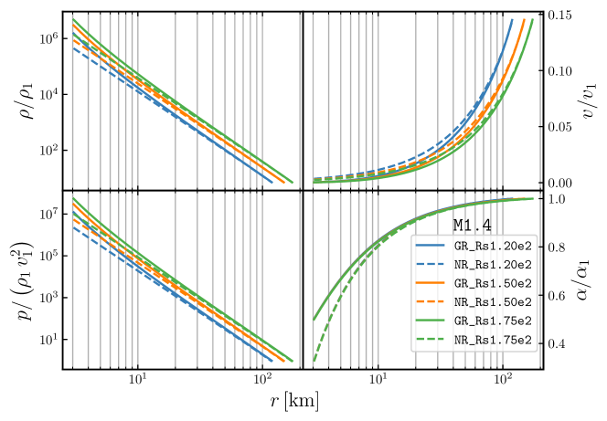
Figure 1: Post-shock, steady-state solutions for GR (solid) and NR (dashed) equations as functions of coordinate distance $r\in\left[3\,\mathrm{km},R_{\textsc{s}}\right]$ for three models having the same accretion rate of 0.3$\,M_{\odot}/\mathrm{s}$, the same PNS mass of 1.4$\,M_{\odot}$, and shock radii 120 km (blue), 150 km (orange), and 175 km (green). For this PNS mass, the Schwarzchild radius is $\sim$1 km. Quantities defined just ahead of the shock are denoted with a subscript “1”. The top-left panel shows the comoving baryon mass density normalized to its value just ahead of the shock, the top-right panel shows the radial component of the fluid three-velocity normalized to its value just ahead of the shock, the bottom-left panel shows the comoving pressure normalized to the Newtonian ram pressure just ahead of the shock, $\rho_{1}\,v_{1}^{2}$, and the bottom right panel shows the lapse function (solid) and the Newtonian approximation to the lapse function (dashed), $1+\Phi$, with $\Phi$ the Newtonian gravitational potential, normalized to their values at the shock.

For the high-compactness case (e.g., see Liebendörfer et al., 2001; Walk et al., 2020), Figure 2 shows steady-state accretion shock solutions as functions of coordinate distance $r$, with $M_{\textsc{pns}}=2.8\,M_{\odot}$, $\dot{M}=0.3\,M_{\odot}\,\mathrm{s}^{-1}$, and $R_{\textsc{s}}/\mathrm{km}\in\left\{60,70\right\}$. The profiles show the same trends as those in Figure 1, although in this case the trends are more pronounced. One notable difference is that the location of the largest deviation in the velocity between the NR and GR cases occurs further in, near $r=12~{}\mathrm{km}$. Another notable feature of both Figures 1 and 2 is that the fluid velocity in the GR case is consistently slower than that in the NR case, in agreement with Kundu & Coughlin (2022).

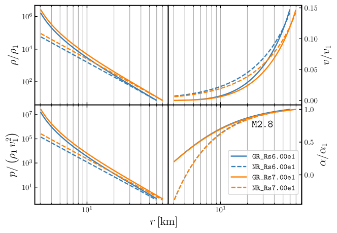
Figure 2: Post-shock, steady-state solutions for GR (solid) and NR (dashed) equations as functions of coordinate distance $r\in\left[3\,\mathrm{km},R_{\textsc{s}}\right]$ for three models having the same accretion rate of 0.3$\,M_{\odot}/\mathrm{s}$, the same PNS mass of $2.8\,M_{\odot}$, and shock radii 60 km (blue) and 70 km (orange). For this PNS mass, the Schwarzchild radius is $\sim$2.1 km. Quantities defined just ahead of the shock are denoted with a subscript “1”. The top-left panel shows the comoving baryon mass density normalized to its value just ahead of the shock, the top-right panel shows the radial component of the fluid three-velocity normalized to its value just ahead of the shock, the bottom-left panel shows the comoving pressure normalized to the Newtonian ram pressure just ahead of the shock, $\rho_{1}\,v_{1}^{2}$, and the bottom right panel shows the lapse function (solid) and the Newtonian approximation to the lapse function (dashed), $1+\Phi$, with $\Phi$ the Newtonian gravitational potential, normalized to their values at the shock.

We compare our numerical results with an estimate provided by Müller (2020), which provides an analytic estimate of the oscillation period of the SASI, $T_{\mathrm{aa}}$, based on the assumption that the SASI is an advective-acoustic cycle, in which a fluid parcel advects from the shock to the PNS surface in time $\tau_{\mathrm{ad}}$, which generates acoustic waves that propagate from the PNS surface to the shock in time $\tau_{\mathrm{ac}}$. We modify that formula to include the effects of GR by including the metric factor, which involves the conformal factor and which converts the radial coordinate increment to the proper radial distance increment, and by replacing the non-relativistic signal-speeds with their relativistic counterparts,

$$T_{\mathrm{aa}}\approx\tau_{\mathrm{ad}}+\tau_{\mathrm{ac}}=\int\limits_{R_{\textsc{s}}}^{R_{\textsc{pns}}}\frac{\sqrt{\gamma_{11}}\,dr}{\lambda^{r}_{0}}+\int\limits_{R_{\textsc{pns}}}^{R_{\textsc{s}}}\frac{\sqrt{\gamma_{11}}\,dr}{\lambda^{r}_{+}},$$ (26)

where $\lambda^{r}_{0}$ and $\lambda^{r}_{+}$ are the radial signal-speeds of matter and acoustic waves, respectively. Using our metric, the signal-speeds are (Rezzolla & Zanotti, 2013)

$$\lambda^{r}_{0} =\alpha\,v^{r} \stackrel{{\scriptstyle\textsc{nr}}}{{=}}v^{r},$$ (27)

$$\lambda^{r}_{+} =\frac{\alpha}{1-v^{i}v_{i}\,c_{s}^{2}}\left\{v^{r}\left(1-c_{s}^{2}\right)+c_{s}\sqrt{\left(1-v^{i}v_{i}\right)\left[\gamma^{11}\left(1-v^{i}v_{i}\,c_{s}^{2}\right)-v^{r}\,v^{r}\left(1-c_{s}^{2}\right)\right]}\right\} \stackrel{{\scriptstyle\textsc{nr}}}{{=}}v^{r}+c_{s},$$ (28)

where $c_{s}$ is the sound-speed and where the second equality in each expression is the non-relativistic limit. For 1D problems, this expression depends only on the steady-state values of $c_{s}$ and $v^{r}$. We also compare our results with an estimate based on the assumption that the SASI is a purely acoustic phenomenon. We define a time, $T_{\mathrm{ac}}$, as the time taken by an acoustic perturbation to circumnavigate the PNS at a characteristic radius $R_{\mathrm{ac}}$, assuming $v^{\theta}\ll c_{s}\,\sqrt{\gamma^{22}}$,

$$T_{\mathrm{ac}}:=2\pi\,R_{\mathrm{ac}}/\left(h_{\theta}\,\lambda_{+}^{\theta}\right),$$ (29)

where

$$\lambda^{\theta}_{+}=\frac{\alpha}{1-v^{i}v_{i}\,c_{s}^{2}}\left\{v^{\theta}\left(1-c_{s}^{2}\right)+c_{s}\sqrt{\left(1-v^{i}v_{i}\right)\left[\gamma^{22}\left(1-v^{i}v_{i}\,c_{s}^{2}\right)-v^{\theta}\,v^{\theta}\left(1-c_{s}^{2}\right)\right]}\right\}\stackrel{{\scriptstyle\textsc{nr}}}{{=}}v^{\theta}+c_{s}/r$$ (30)

is the acoustic wave-speed in the $\theta$-dimension (Rezzolla & Zanotti, 2013), $h_{\theta}$ is the scale factor in the $\theta$-dimension.

We plot, in Figure 3, $\lambda^{r,\textsc{gr}}_{+}/\lambda^{r,\textsc{nr}}_{+}$, $\lambda^{\theta,\textsc{gr}}_{+}/\lambda^{\theta,\textsc{nr}}_{+}$, and $\lambda^{r,\textsc{gr}}_{0}/\lambda^{r,\textsc{nr}}_{0}$ as functions of $\eta$, defined as

$$\eta\left(r\right):=\left(r-R_{\textsc{pns}}\right)/\left(R_{\textsc{s}}-R_{\textsc{pns}}\right),$$ (31)

for all of our models. In all cases, the signal-speeds are slower in the GR case. This difference is accentuated in the high-compactness suite and for smaller radii.

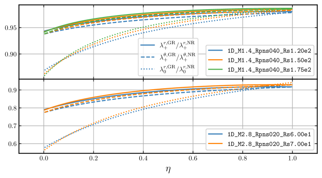
Figure 3: Ratio of radial GR acoustic signal-speed to radial NR acoustic signal-speed (solid), ratio of angular GR acoustic signal-speed to angular NR acoustic signal-speed (dashed), and ratio of radial GR advective signal-speed to radial NR advective signal-speed (dotted), plotted as functions of $\eta$ for all models. Low-compactness models are shown in the top panel and high-compactness models are shown in the bottom panel. All signal-speeds have been multiplied with the appropriate scale factors.

The growth rate of the SASI depends on the steady-state conditions below the shock; however, obtaining an analytic estimate for this is difficult, and although there have been efforts to explain the physics governing the growth rate assuming non-relativistic models (e.g., Blondin & Mezzacappa, 2006; Foglizzo et al., 2007; Laming, 2007, 2008; Foglizzo, 2009; Guilet & Foglizzo, 2012), an analytic estimate remains an open question and no estimate exists for a GR model. Here, we aim to compare the NR and GR growth rates with numerical simulations.

We emphasize that our goal is to characterize the SASI in terms of its period and growth rate, and to compare their GR and NR values. Determining its physical origin, whether it be advective-acoustic or purely acoustic, is beyond the scope of this study. The rough estimates provided by (26) and (29) are merely intended as points of reference for our numerically determined values.

4 Simulation Code and Setup

We perform our simulations with thornado, an open-source code under development, aiming to simulate CCSNe. thornado uses high-order discontinuous Galerkin (DG) methods to discretize space and strong-stability-preserving Runge–Kutta methods to evolve in time. For details on the implementation in the non-relativistic case, see Endeve et al. (2019) and Pochik et al. (2021). In the relativistic case, see Dunham et al. (2020) and Dunham et al. (2023) (in prep.). All of our simulations use the HLL Riemann solver (Harten et al., 1983), a quadratic polynomial representation (per dimension) of the solution in each element, and third-order SSP-RK methods for time integration (Gottlieb et al., 2001) with a timestep $\Delta t:=C_{\textsc{cfl}}\frac{1}{d\left(2\,k+1\right)}\min\limits_{i\in\left\{1,\cdots,d\right\}}\Delta x^{i}/\left|\lambda^{i}\right|$, where $C_{\textsc{cfl}}=0.5$ is the CFL number, $k$ the degree of the approximating polynomial (in our case, $k=2$), $\Delta x^{i}$ the mesh width in the $i$-th dimension, $\lambda^{i}$ the fastest signal-speed in the $i$-th dimension, and $d$ the number of spatial dimensions (Cockburn & Shu, 2001).

Two important aspects of successful implementations of the DG method are mitigating spurious oscillations and enforcing physical realizability of the polynomial approximation of the solution. To mitigate oscillations, thornado uses the minmod limiter and applies it to the characteristic fields (see, e.g., Shu, 1987; Pochik et al., 2021). For the interested reader, we set the $\beta_{\textsc{tvd}}$ parameter for the limiter, defined in Pochik et al. (2021), to $1.75$ for all runs. thornado also uses the troubled-cell indicator described in Fu & Shu (2017) to decide on which elements to apply the minmod limiter; for the threshold of that indicator we use the value $5\times 10^{-3}$. To enforce physical realizability of the solution in the NR case, thornado uses the positivity limiter described in Zhang & Shu (2010), and in the GR case, uses the limiter described in Qin et al. (2016); for the thresholds of both limiters we use the value $10^{-13}$.

The hydrodynamics in thornado has recently been coupled to AMReX, an open-source software library for block-structured adaptive mesh refinement and parallel computation with MPI (Zhang et al., 2019); however, our simulations are all performed on a uni-level mesh.

Our computational domain, $\mathcal{D}$, is defined for all models as $\mathcal{D}:=\left[R_{\textsc{pns}},1.5\,R_{\textsc{s}}\left(t=0\right)\right]\times\left[0,\pi\right]$. The radial extent allows us to determine whether or not the SASI has become nonlinear, which we define to be when any radial coordinate of the shock exceeds $10\%$ of the initial shock radius. All simulations are evolved sufficiently long to achieve ten full cycles of the SASI. In some cases, the shock exceeds our threshold of nonlinearity before completing ten full cycles; in those cases, we only use data from the linear regime.

The PNS is treated as a fixed, spherically symmetric mass in order to maintain a steady-state, and we ignore the self-gravity of the fluid. Because the largest accretion rate we consider is $0.5\,M_{\odot}\,\mathrm{s}^{-1}$ and because this lasts for a maximum of $550\,\mathrm{ms}$ in our 2D models, the most mass that would accrete onto the PNS is $0.275\,M_{\odot}$ and therefore would provide a sub-dominant contribution to $M_{\textsc{pns}}$ in our simulations.

We consider models with three free parameters: the mass of the PNS, $M_{\textsc{pns}}$, the radius of the PNS, $R_{\textsc{pns}}$, and the initial radius of the shock, $R_{\textsc{s}}$. We also varied the mass accretion rate, $\dot{M}$, but found that the oscillation periods and growth rates to be insensitive to this parameter, and we do not discuss these models further; all following discussion is for models with an accretion rate $\dot{M}=0.3\,M_{\odot}\,\mathrm{s}^{-1}$. Our choice of parameters is motivated by the physical scale of CCSNe; the ranges of our parameter space are informed by models from Liebendörfer et al. (2001); Bruenn et al. (2013); Melson et al. (2015b); Burrows et al. (2020); Walk et al. (2020), and can be found in Table 1. We also classify our simulations by their compactness, $\xi$, which we define as (O’Connor & Ott, 2011),

$$\xi:=\frac{M/M_{\odot}}{R_{\textsc{pns}}/\left(20\,\mathrm{km}\right)}.$$ (32)

One suite, which we refer to as “low-compactness”, has $\xi=0.7$; the other suite, which we refer to as “high-compactness”, has $\xi=2.8$. We vary $M_{\textsc{pns}}$ and $R_{\textsc{pns}}$ in such a way as to ensure these two values of compactness.

Table 1: Model Parameters

Model	$M_{\textsc{pns}}\left[M_{\odot}\right]$	$R_{\textsc{pns}}\left[\mathrm{km}\right]$	$R_{\textsc{s}}\left[\mathrm{km}\right]$	$\xi$
M1.4_Rpns040_Rs1.20e2	1.4	40	120	0.7
M1.4_Rpns040_Rs1.50e2	1.4	40	150	0.7
M1.4_Rpns040_Rs1.80e2	1.4	40	180	0.7
M2.8_Rpns020_Rs6.00e1	2.8	20	60	2.8
M2.8_Rpns020_Rs7.00e1	2.8	20	70	2.8

Note. — Model parameters chosen for the 5 models. All models were run with both GR and NR. The first three rows correspond to the low-compactness models and the last two rows correspond to the high-compactness models.

In our model naming convention, we first list whether the model used GR or NR along with the dimensionality (1D or 2D), followed by the mass of the PNS in Solar masses, the radius of the PNS in kilometers, and lastly the shock radius in kilometers; e.g., the 2D GR model with $M_{\textsc{pns}}=1.4\,M_{\odot}$, $R_{\textsc{pns}}=40\,\mathrm{km}$, and $R_{\textsc{s}}=150\,\mathrm{km}$ is named GR2D_M1.4_Rpns040_Rs1.50e2. If we compare an NR model with a GR model having the same parameters we may drop that specification from the model name. If no confusion will arise, we may also drop the dimensionality.

The inner radial boundary corresponds to the surface of the PNS. To determine appropriate inner-boundary conditions in the GR case, we assume $D$ and $\tau$ follow power laws in radius; from the initial conditions, we extrapolate $D$ and $\tau$ in radius using a least-squares method with data from the innermost five elements on the grid to determine the appropriate exponents. The radial momentum density interior to $R_{\textsc{pns}}$ is kept fixed to its initial value. We leave the outer radial boundary values fixed to their initial values for all fields. In the polar direction, we use reflecting boundary conditions at both poles. For the inner-boundary conditions in the non-relativistic case, we assume $\rho\left(r\right)\propto r^{-3}$ and $E\left(r\right)\propto r^{-4}$, the latter of which follows from our assumption of $\rho\propto r^{-3}$, (13), (14), the assumption of $\Gamma=4/3$, and the assumption of a small velocity at the PNS surface.

For the low-compactness conditions we enforce a radial resolution of 0.5 km per element for all runs, which we found necessary for the shock in an unperturbed model to not deviate by more than 1% over 100 advection times. This is shown in the top panel of Figure 4, which plots the relative deviation of the shock radius from its initial position as a function of $t/\tau_{\mathrm{ad}}$ for runs with different radial resolutions for model GR1D_M1.4_Rpns040_Rs1.20e2. These results suggest that the steady-state is not maintained if the radial resolution is too coarse; e.g., greater than about 1 km.

For the high-compactness conditions we enforce a radial resolution of 0.25 km per element for all runs in order to maintain the same radial resolution of the pressure scale height, $p\left|dp/dr\right|^{-1}$, as in the low-compactness models, while also ensuring that the shock does not deviate from its initial location by more than 1%. This can be seen in the bottom panel of Figure 4, which plots the same quantity as the top panel, but for model GR1D_M2.8_Rpns020_Rs6.00e1.

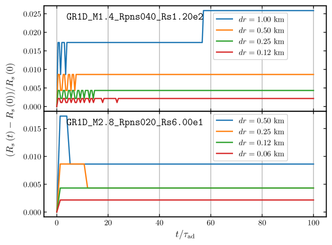
Figure 4: Relative deviation of the shock radius from its initial location versus $t/\tau_{\mathrm{ad}}$ for different radial resolutions $dr$ for the low-compactness model GR1D_M1.4_Rpns040_Rs1.20e2 (top panel) and the high-compactness model GR1D_M2.8_Rpns020_Rs6.00e1 (bottom panel).

To verify that our chosen angular resolution of 64 elements ($\sim$2.8^∘) is sufficient to resolve the angular variations of the fluid, we run two additional simulations of model NR2D_M2.8_Rpns040_Rs1.20e2, one with 128 angular elements and one with 256 angular elements. From those runs, we extract the best-fit values for the growth rates and oscillation periods (see § 5) and find them to not significantly differ from those of the 64-angular-element run.

Our simulations are initialized with the steady-state solutions discussed in § 3, and we take extra care to minimize initial transients. The initial conditions we obtain come from solving Eqs. (14), (20), and (21) in the GR case, and Eqs. (14), (24), and (25) in the NR case, which are not exact solutions of our discretized equations, so transients will be present when simulations are initialized with these solutions. To mitigate the effects of the transients, the fields are set up in 1D with the method described above and then evolved for 100 advection times, which was experimentally determined to be of sufficient duration to quell any transients. We verify that the system has achieved a steady-state by plotting, in Figure 5, the maximum, at each snapshot, of the absolute value of the normalized time derivative of the mass density versus $t/\tau_{\mathrm{ad}}$ for low-compactness model GR1D_M1.4_Rpns040_Rs1.20e2 (top panel) and high-compactness model GR1D_M2.8_Rpns020_Rs6.00e1 (bottom panel); other models exhibit similar behavior. It can be seen that the low-compactness model settles down after approximately 35 advection times, followed by two slight increases near 45 and 50 advection times, then settles down until we end the simulation after 100 advection times. We attribute the two slight increases to limiters activating when the shock crosses an element boundary.

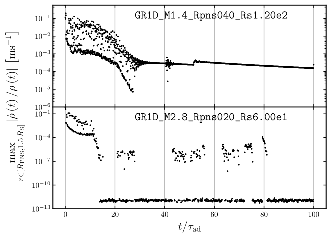
Figure 5: Maximum, at each snapshot, of the absolute value of the normalized time derivative of the mass density versus $t/\tau_{\mathrm{ad}}$ for low-compactness model GR1D_M1.4_Rpns040_Rs1.20e2 (top panel) and high-compactness model GR1D_M2.8_Rpns020_Rs6.00e1 (bottom panel).

The relaxed 1D data is mapped to 2D, a perturbation to the pressure is applied (see below), and the system is evolved. The initial relaxation in 1D removes numerical noise and allows for a smaller perturbation amplitude, leading to a longer-lasting linear regime, which makes for a cleaner signal.

We seed the instability by imposing a pressure perturbation onto the steady-state flow below the shock,

$$p\left(r,\theta\right)=p\left(r\right)+\delta p\left(r,\theta\right),$$ (33)

with $p\left(r\right)$ the steady-state pressure at radius $r$, and where $\delta p\left(r,\theta\right)/p\left(r\right)$ is defined in a scale-independent manner as

$$\frac{\delta p\left(r,\theta\right)}{p\left(r\right)}:=10^{-6}\,\ \exp\left(\frac{-\left(\eta-\eta_{\mathrm{c}}\right)^{2}}{2\,\sigma^{2}}\right)\,\cos\theta,$$ (34)

with $\eta$ defined in (31), and where $\eta_{\mathrm{c}}=0.75$ and $\sigma=0.05$. The perturbation is not allowed to extend into the pre-shock flow. We opted to perturb the post-shock flow as opposed to the pre-shock flow after having tried various pre-shock and post-shock perturbations and finding that pre-shock perturbations generate noise when they cross the shock front, thus creating a noisy signal and making it more difficult to extract quantities of interest. Similarly, we choose a Gaussian profile because the smoothness of the profile generates less noise than, e.g., a top-hat profile. The $\cos\theta$ factor is meant to excite an $\ell=1$ Legendre mode of the SASI. While this perturbation method does not exactly mimic the hydrodynamics inside a CCSN, it is sufficient to study the SASI in the linear regime.

5 Results and Discussion

Here we discuss our analysis methods and compare the SASI growth rates and oscillation periods for our 5 models in GR and NR.

5.1 Analysis Methods

To extract SASI growth rates from our simulations, we follow Blondin & Mezzacappa (2006) and expand a quantity affected by the perturbed flow, $A\left(t,r,\theta\right)$, in Legendre polynomials,

$$A\left(t,r,\theta\right)=\sum\limits_{\ell=0}^{\infty}G_{\ell}\left(t,r\right)\,P_{\ell}\left(\cos\theta\right),$$ (35)

where we normalize the $P_{\ell}$ such that

$$\int\limits_{-1}^{1}P_{\ell}\left(x\right)\,P_{\ell^{\prime}}\left(x\right)\,dx=\delta_{\ell\ell^{\prime}},$$ (36)

with $\delta_{\ell\ell^{\prime}}$ the Kronecker delta function. Then,

$$G_{\ell}\left(t,r\right):=\int\limits_{-1}^{1}A\left(t,r,\theta\right)\,P_{\ell}\left(\cos\theta\right)\,d\left(\cos\theta\right)=\int\limits_{0}^{\pi}A\left(t,r,\theta\right)\,P_{\ell}\left(\cos\theta\right)\,\sin\theta\,d\theta.$$ (37)

After experimenting with several quantities, we decided to use the quantity proposed by Scheck et al. (2008),

$$A\left(t,r,\theta\right):=\frac{1}{\sin\theta}\,\frac{\partial}{\partial\theta}\left(v^{\theta}\left(t,r,\theta\right)\,\sin\theta\right),$$ (38)

where $v^{\theta}$ is the fluid velocity in the polar direction as measured by an Eulerian observer, having units of $\mathrm{rad}\,\mathrm{s}^{-1}$. With $G_{\ell}$, we compute the power in the $\ell$-th Legendre mode, $H_{\ell}\left(t\right)$, by integrating over a shell below the shock, bounded from below by $r_{a}=0.8\,R_{\textsc{s}}$ and from above by $r_{b}=0.9\,R_{\textsc{s}}$,

$$H_{\ell}\left(t\right):=\int\limits_{0}^{2\pi}\int\limits_{0}^{\pi}\int\limits_{r_{a}}^{r_{b}}\left[G_{\ell}\left(t,r\right)\right]^{2}\left[\psi\left(r\right)\right]^{6}r^{2}\,\sin\theta\,dr\,d\theta\,d\varphi=4\pi\int\limits_{r_{a}}^{r_{b}}\left[G_{\ell}\left(t,r\right)\right]^{2}\left[\psi\left(r\right)\right]^{6}r^{2}\,dr.$$ (39)

For the Newtonian runs, $\psi=1$. We experimented with different values of $r_{a}$ and $r_{b}$ and found that a thin shell just below the shock gave the cleanest signal.

To extract the SASI growth rate and oscillation period from $H_{1}$, we begin by fitting the simulation data to the function (Blondin & Mezzacappa, 2006)

$$F_{1}\left(t\right)=F\,e^{2\,\omega\,t}\,\sin^{2}\left(\frac{2\pi}{T}\,t+\delta\right),$$ (40)

where $\omega$ is the growth rate of the SASI, $T$ is the oscillation period of the SASI, $F$ is an amplitude, and $\delta$ is a phase offset.

We fit the data to the model using the Levenberg–Marquardt nonlinear least squares method (e.g., see Moré, 1978), provided by scipy’s curve_fit function, which also provides an estimate on the uncertainty of the fit via the diagonal entries of the covariance matrix; we use this to define the uncertainty in the growth rate. The temporal extent over which we perform the fit is defined to begin after one SASI oscillation and to end after seven SASI oscillations, where, for simplicity, we use (26) to define the period of one SASI oscillation.

The period we report is obtained by performing a Fourier analysis: We integrate the lateral flux in the radial direction,

$$F^{r}_{\theta}=\sqrt{\gamma}\,\rho\,v^{r}\,v_{\theta}\times\alpha\,h\,W^{2}\stackrel{{\scriptstyle\textsc{nr}}}{{=}}\sqrt{\gamma}\,\rho\,v^{r}\,v_{\theta},$$ (41)

from $r_{a}$ to $r_{b}$ (defined as in the computation of the $H_{\ell}$), integrate the result over $\mathbb{S}^{2}:=\left\{\left(\theta,\varphi\right)\in\mathbb{R}^{2}\big{|}\theta\in\left[0,\pi\right],\varphi\in\left[0,2\pi\right)\right\}$, and then take the Fourier transform of that result using the fft tool from scipy. From the result, $\widetilde{F}^{r}_{\theta}(\widetilde{T})$, we define the period of the SASI as the value of $\widetilde{T}$ corresponding to the peak of the Fourier amplitudes, and we define the uncertainty in the period as the full width at half maximum (FWHM) of the Fourier amplitudes. The FFT is computed over the same time interval as the aforementioned fit. (We do not use the period returned from curve_fit because, for some models, pollution from higher-order modes spoils the ability of our fitting function to capture the $\ell=1$ mode.)

5.2 Overall Trends

Here we discuss trends that appear across both the low-compactness models and the high-compactness models. We summarize our results in Table 2, which lists the model, the best-fit oscillation period and uncertainty, the best-fit growth rate and uncertainty, the product of the best-fit growth rate and best-fit oscillation period, the period assuming an advective-acoustic mechanism (estimated using (26)), and the period assuming a purely acoustic mechanism (estimated using (29)). Due to data uncertainties, and the similar values provided by the two estimates, we are unable to discern whether the SASI is governed by an advective-acoustic mechanism or by a purely acoustic mechanism using these simple estimates.

Table 2: Results

Model	$T\pm\Delta T\,\left[\mathrm{ms}\right]$	$\omega\pm\Delta\omega\,\left[\mathrm{ms}^{-1}\right]$	$\omega\,T$	$T_{\mathrm{aa}}\,\left[\mathrm{ms}\right]$	$T_{\mathrm{ac}}\,\left[\mathrm{ms}\right]$
NR_M1.4_Rpns040_Rs1.20e2	23.7044 $\pm$ 11.9819	0.0733 $\pm$ 0.0011	1.7368	20.8348	26.2646
GR_M1.4_Rpns040_Rs1.20e2	27.0412 $\pm$ 14.3661	0.0578 $\pm$ 0.0011	1.5623	23.6236	26.9372
NR_M1.4_Rpns040_Rs1.50e2	37.1673 $\pm$ 22.3333	0.0409 $\pm$ 0.0005	1.5209	34.3279	36.6791
GR_M1.4_Rpns040_Rs1.50e2	40.2225 $\pm$ 22.3889	0.0360 $\pm$ 0.0004	1.4491	38.6747	37.4293
NR_M1.4_Rpns040_Rs1.75e2	51.1234 $\pm$ 23.4707	0.0300 $\pm$ 0.0003	1.5341	47.7212	46.0841
GR_M1.4_Rpns040_Rs1.75e2	57.6475 $\pm$ 25.9759	0.0265 $\pm$ 0.0003	1.5274	53.5372	46.8924
NR_M2.8_Rpns020_Rs6.00e1	6.1049 $\pm$ 4.1534	0.2910 $\pm$ 0.0085	1.7767	5.2343	6.5656
GR_M2.8_Rpns020_Rs6.00e1	7.5868 $\pm$ 2.4527	0.1365 $\pm$ 0.0042	1.0360	8.6607	7.2635
NR_M2.8_Rpns020_Rs7.00e1	7.9656 $\pm$ 3.6955	0.1897 $\pm$ 0.0054	1.5113	7.4177	8.2693
GR_M2.8_Rpns020_Rs7.00e1	10.2503 $\pm$ 3.2875	0.0954 $\pm$ 0.0026	0.9781	12.1099	9.0178

Note. — Oscillation periods, growth rates, and their uncertainties for all ten models having the same accretion rate of $0.3\,M_{\odot}\,\mathrm{s}^{-1}$. The first six are the low-compactness models; the last four are the high-compactness models. The uncertainties for the growth rates are defined as the square roots of the diagonal entries of the covariance matrix corresponding to the growth rate. The uncertainies for the oscillation period are defined as the full-width half-maximum values of the Fourier amplitudes (see Figure 6). The fourth column shows the product of the best-fit growth rate multiplied by the best-fit oscillation period. The fifth column shows the estimate for the period assuming an advective-acoustic origin of the SASI ((26)), and the sixth column shows the estimate for the period assuming a purely acoustic origin of the SASI ((29)), where we use $R_{\mathrm{ac}}=0.85\,R_{\textsc{s}}$, the midpoint of the shell in which we compute the power (see § 5).

As a first general trend, we see that, for a given PNS radius, the oscillation period increases as the shock radius increases, as seen clearly in the second column of Table 2. This is expected, for as the shock radius increases, the waves supported by the fluid must traverse a larger region, therefore each cycle will take longer. As a second general trend, we observe that, for a given PNS radius, the growth rate decreases as the shock radius increases.

We note that the power injection rate (i.e., the growth rate) per SASI cycle is approximately constant for all low-compactness models and all high-compactness, NR models, and also approximately constant, but with a different mean, for the high-compactness, GR models. Phrased another way, $\omega\,T$ is approximately constant for all models within one of these two groups. This can be seen from the fourth column of Table 2: The values for the low-compactness models and the high-compactness, NR models have a mean of 1.58 with a small scatter, $1.58^{+0.20}_{-0.13}$, while the high-compactness, GR models have a mean of 1.01 with a small scatter, $1.01^{+0.03}_{-0.03}$.

5.3 Impact of GR

Next we discuss the impact of GR on the oscillation period and the growth rate.

5.3.1 Oscillation Period

First we discuss how the oscillation period varies with PNS compactness and shock radius. In Figure 6, we plot the amplitudes of the Fourier transform of (41), $\widetilde{F}^{r}_{\theta}$, versus $\widetilde{T}$ for all models, where $\widetilde{T}$ is defined as the inverse of the frequency determined by the FFT. No windowing was applied when computing the FFT of the signal.

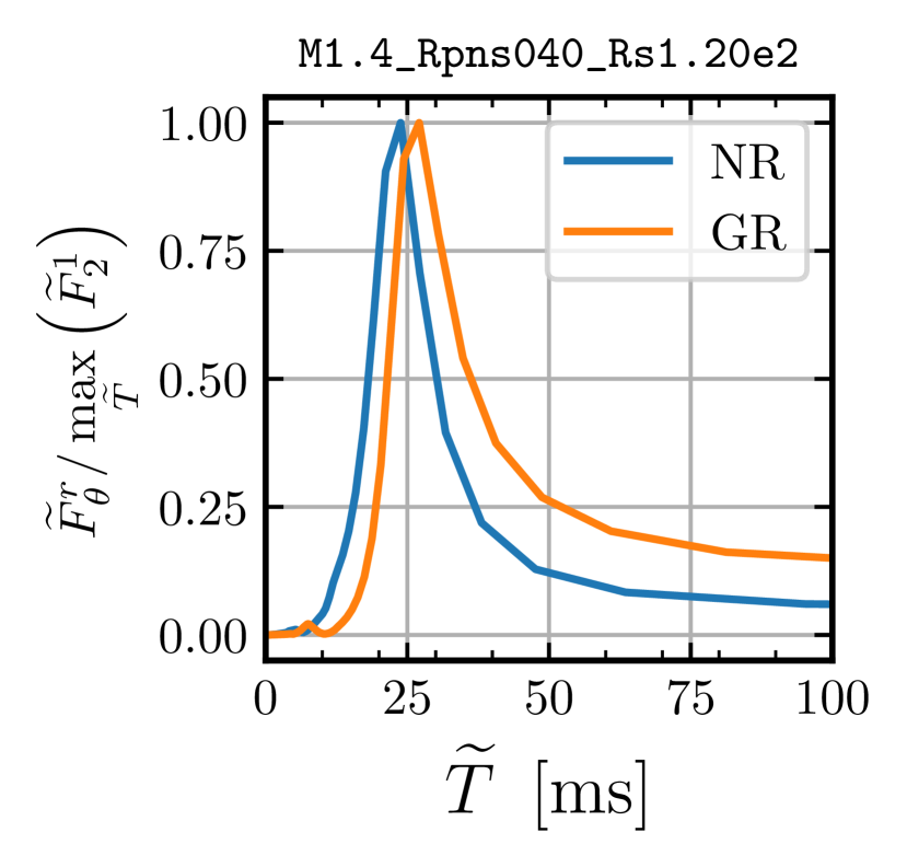
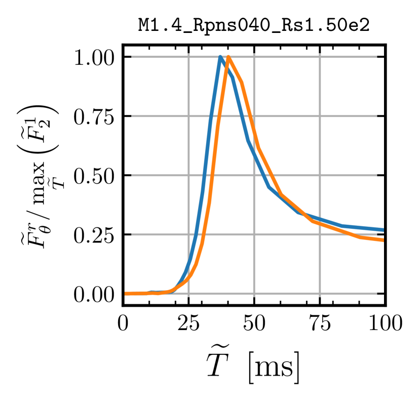
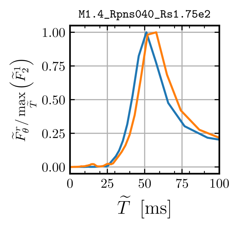
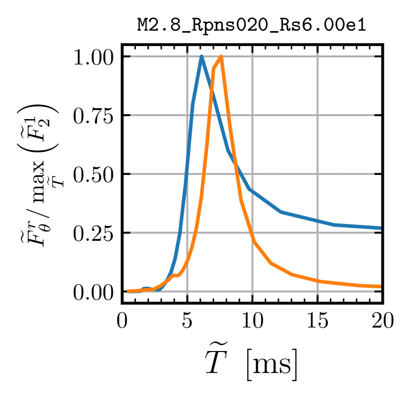
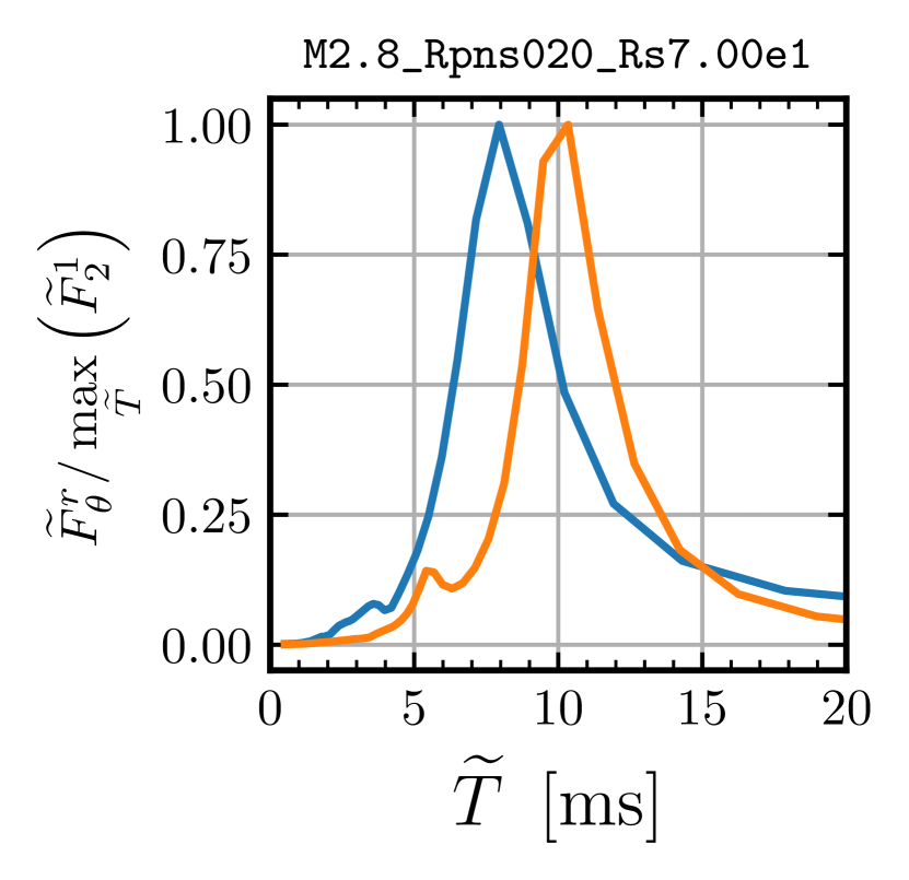
Figure 6: Amplitudes of Fourier transforms of (41), normalized by their largest values, as functions of $\widetilde{T}$ in $\mathrm{ms}$, where $\widetilde{T}$ is the inverse of the frequency returned by the FFT. From left to right, columns correspond to models with increasing shock radii and rows corresponds to low-compactness (top) and high-compactness (bottom) models. NR results are shown in blue and GR results are shown in orange.

We see that the difference in the optimal period, $T$ (defined as the $\widetilde{T}$ associated with the largest Fourier amplitude), between NR and GR increases with increasing compactness, with the GR period consistently longer than the NR period. This can be explained by differences in the structure of the post-shock solutions; in particular, the signal-speeds, which are shown in Figure 3. Both the radial acoustic and advective signal-speeds, as well as the angular acoustic signal-speed, are consistently smaller in GR. Because of this, the period is longer for a given model when GR is used, regardless of whether the SASI is governed by an advective-acoustic or a purely acoustic cycle.

In Figure 7, we plot the estimates for the period provided by Eqs. (26) and (29), along with the period and its uncertainty provided by the Fourier analysis, versus initial shock radius for all the models.

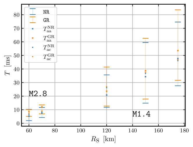
Figure 7: SASI oscillation period and uncertainty in $\mathrm{ms}$ as a function of PNS mass and shock radius in $\mathrm{km}$, as determined by the FFT (see text for details). NR results are shown in blue and GR results are shown in orange. Crosses correspond to estimates of the period assuming the SASI is governed by an advective-acoustic mechanism ((26)) using the GR data and the GR part of (26) (orange) and using the NR data and the NR part of (26) (blue). Filled circles correspond to estimates of the period assuming the SASI is governed by a purely acoustic mechanism ((29)).

The NR and GR models, along with their associated estimates, follow the same general trends. For the low-compactness models, we find that the ratio between $T_{\textsc{gr}}$ and $T_{\textsc{nr}}$ is as large as 1.14, the relative difference between $T_{\textsc{gr}}$ and the advective-acoustic estimate, (26), is smaller than 13%, and the relative difference between $T_{\textsc{gr}}$ and the purely acoustic estimate, (29), is smaller than 21%. For the high-compactness models, we find that the ratio between $T_{\textsc{gr}}$ and $T_{\textsc{nr}}$ is as large as 1.29, the relative difference between $T_{\textsc{gr}}$ and the advective-acoustic estimate, (26), is smaller than 17%, and the relative difference between $T_{\textsc{gr}}$ and the purely acoustic estimate, (29), is smaller than 13%.

5.3.2 Growth Rate

Next we discuss how the growth rate varies with PNS compactness and shock radius. In Figure 8, we plot the power in the first Legendre mode, $H_{1}$, during the linear regime, as a function of time in milliseconds for all our models.

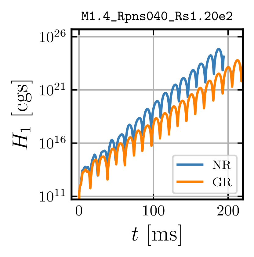
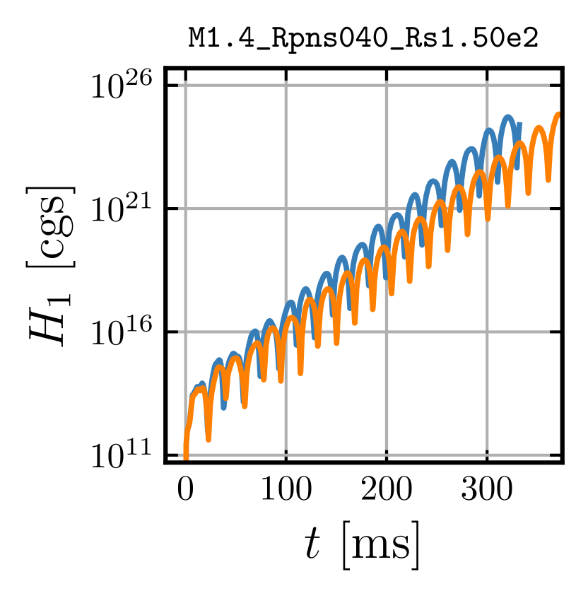
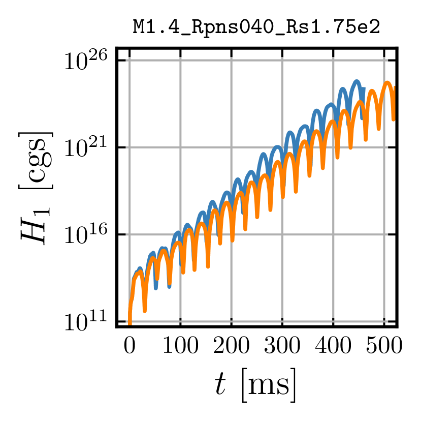
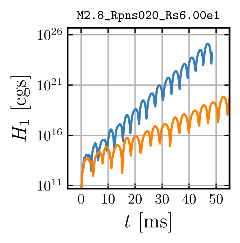
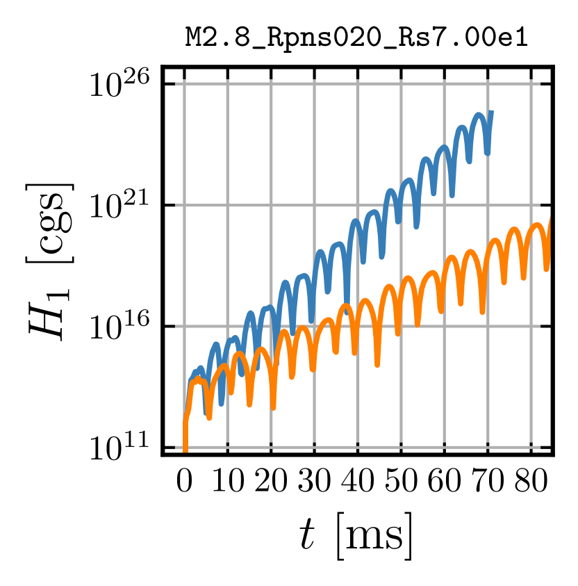
Figure 8: $H_{1}$ in cgs units versus $t$ in $\mathrm{ms}$. The layout of the panels is the same as in Figure 6: From left to right, columns correspond to models with increasing shock radii and rows correspond to low-compactness (top) and high-compactness (bottom) models. NR results are shown in blue and GR results are shown in orange. Note that the horizontal axis limits are different in each panel.

For all models displayed here, the shock deviates from spherical symmetry by less than 10%, and we consider this sufficient for characterizing the evolution as being in the linear regime.

We see a clear trend in the growth rate: the GR models display a slower SASI growth rate when compared to their NR counterparts. In Figure 8, it can be seen that, even for the low-compactness models, GR has a non-negligible effect on the growth rate. This effect is a function of shock radius, with a smaller shock radius leading to a larger difference in the NR and GR growth rates. This effect is drastically enhanced when going from the low-compactness models to the high-compactness models. In the high-compactness models, the power in the $\ell=1$ mode is some five orders of magnitude lower in the GR case by the end of the simulation (see Figure 8). The effects of GR can also be seen in Figure 9, which plots the growth rate for all models as a function of $R_{\textsc{s}}$.

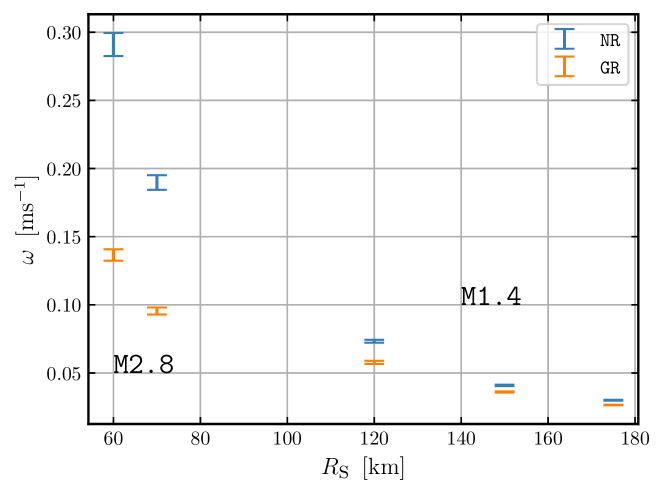
Figure 9: SASI growth rate and uncertainty in $\mathrm{ms}^{-1}$ as a function of shock radius in $\mathrm{km}$, as determined by the fit to (40) (see text for details). NR results are shown in blue and GR results are shown in orange.

Again, in all cases, the growth rate is slower for the GR models and the difference between GR and NR growth rates increases with decreasing shock radius and increasing PNS mass – i.e., under more relativistic conditions – the ratio becoming as small as 0.47.

In Figure 10, we again plot $H_{1}$, but this time as a function of $t/T$. (When interpreting this figure, note that $T$ is different for each model.)

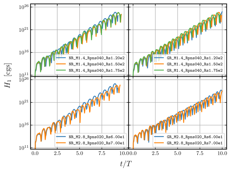
Figure 10: $H_{1}$ in cgs units versus $t/T$. The top-left panel shows the low-compactness, NR models, the top-right panel shows the low-compactness, GR models, the bottom-left panel shows the high-compactness, NR models, and the bottom-right panel shows the high-compactness, GR models.

This figure demonstrates that the growth rate per oscillation period is approximately constant for a given physical model (NR or GR) and compactness. Further, all the low-compactness models (both NR and GR) and the NR high-compactness models reach about the same total power of $\sim$10²⁵ after ten oscillations, while the high-compactness GR models reach a maximum of $\sim$10²³, demonstrating that GR modifies both the oscillation period and the growth rate, but modifies them in such a way as to keep $\omega\,T$ roughly constant for each of these groupings of models.

6 Summary, Conclusion, and Future Work

We examined the effect of GR on 5 idealized, axisymmetric models of the standing accretion shock instability (SASI) by performing a parameter study in which we systematically varied the initial shock radius, along with the mass and radius of the proto-neutron star (PNS); i.e., the compactness of the PNS. We compared these runs by measuring the growth rate and oscillation period of the SASI for all models, which were run once with NRHD and Newtonian gravity and once with GRHD and GR gravity. We set up our simulations to excite a clean $\ell=1$ Legendre mode, computed the power of the SASI in that mode within a thin shell just below the shock, and, following Blondin & Mezzacappa (2006), fit the resulting signal to (40). From the fits, we computed the growth rates and their uncertainties, and using the FFT, we computed the oscillation periods and their uncertainties.

For the low-compactness ($\xi=0.7$) models, we found that the period of the SASI in the GR case is larger than that of the SASI in the NR case, with a ratio between the two as large as $\sim$1.14. For the high-compactness ($\xi=2.8$) models, we found that the period of the SASI in the GR case is larger than that of the SASI in the NR case, with a ratio between the two as large as $\sim$1.29, a significantly larger amount. We explained these differences as resulting from differences in the post-shock flow structure for the GR and NR setups. Our numerically-determined oscillation periods are consistent with simple estimates assuming both advective-acoustic and purely acoustic mechanisms, however, due to uncertainties in numerically-determined oscillation periods, we cannot discern between the two with our data. For all models, we found that the growth rate is slower when GR is used, and significantly slower for the high-compactness models, with the ratio between the GR and NR cases as low as 0.47. We found that both the growth rate and the oscillation period are practically independent of the accretion rate for the range of parameter space we considered.

The connection between our results and the results from realistic core-collapse supernova (CCSN) simulations can be made by considering the trends across all of the models considered here.

First, our results suggest that CCSN simulations based on Newtonian hydrodynamics and Newtonian gravity may fail to predict correctly the growth rate of the SASI and its period of oscillation as conditions below the shock become increasingly relativistic. Under such conditions, the growth rate in the Newtonian case may be overestimated by a factor of two, or more, relative to the GR case. Additionally, the period may be underestimated by about 20%.

Second, as the conditions we considered became increasingly relativistic, the SASI growth rate continued to increase and its period continued to decrease. Thus, our studies provide theoretical support for the conclusions reached in the study of the SASI development in higher-mass progenitors (see, e.g., Hanke et al., 2013; Matsumoto et al., 2022), where the time scales for the development of convection may be long and where the SASI, able to develop on shorter time scales, is able to provide support to the stalled shock, potentially sustaining neutrino heating, and, in turn, the development of neutrino-driven convection, with all of their anticipated benefits for generating an explosion.

Given the substantial impact of GR we find in our simulations, we stress the importance of GR treatments in any future studies aiming to understand the SASI in a CCSN context.

Our results also suggest that CCSN simulations based on Newtonian hydrodynamics and Newtonian gravity may fail to predict correctly the emission of gravitational waves by the SASI (specifically, its frequency and amplitude), a primary target of gravitational wave astronomy given its anticipated existence in that part of frequency space where current-generation gravitational wave detectors such as LIGO and VIRGO are most sensitive. In addition, efforts to discern between contributions from different SASI modes – e.g., sloshing and spiral – may be affected, as well.

In light of the results presented here, further analysis is well motivated. Our assumption of axisymmetry will need to be lifted, since the SASI is known to have non-axisymmetric modes (Blondin & Mezzacappa, 2007; Blondin & Shaw, 2007; Fernández, 2010, 2015). A full three-dimensional comparison of the SASI in NR and GR, such as the one performed here for axisymmetry, should be conducted. Further analyses may also include adding a third type of model that uses NRHD and a GR monopole potential, similar to what is done in several CCSN simulation codes (e.g., Rampp & Janka, 2002; Kotake et al., 2018; Skinner et al., 2019; Bruenn et al., 2020), in order to discern whether the use of an effective potential to capture the stronger gravitational fields present in GR is able to better capture the SASI growth rate and subsequent evolution. Of course, even if it does, nothing can replace a true GR implementation, as we have done here, and as must be done in future CCSN models.

7 Data Availability

The data underlying this paper will be shared on reasonable request to the corresponding author.

References

- Abdikamalov et al. (2015) Abdikamalov, E., Ott, C. D., Radice, D., et al. 2015, ApJ, 808, 70, doi: 10.1088/0004-637X/808/1/70
- Andresen (2017) Andresen, H. 2017, PhD thesis, Munich University of Technology, Germany
- Andresen et al. (2017) Andresen, H., Müller, B., Müller, E., & Janka, H. T. 2017, MNRAS, 468, 2032, doi: 10.1093/mnras/stx618
- Andresen et al. (2019) Andresen, H., Müller, E., Janka, H. T., et al. 2019, MNRAS, 486, 2238, doi: 10.1093/mnras/stz990
- Banyuls et al. (1997) Banyuls, F., Font, J. A., Ibáñez, J. M., Martí, J. M., & Miralles, J. A. 1997, ApJ, 476, 221, doi: 10.1086/303604
- Baumgarte & Shapiro (2010) Baumgarte, T. W., & Shapiro, S. L. 2010, Numerical Relativity: Solving Einstein’s Equations on the Computer (Cambridge University Press)
- Blondin & Mezzacappa (2006) Blondin, J. M., & Mezzacappa, A. 2006, ApJ, 642, 401, doi: 10.1086/500817
- Blondin & Mezzacappa (2007) —. 2007, Nature, 445, 58, doi: 10.1038/nature05428
- Blondin et al. (2003) Blondin, J. M., Mezzacappa, A., & DeMarino, C. 2003, ApJ, 584, 971, doi: 10.1086/345812
- Blondin & Shaw (2007) Blondin, J. M., & Shaw, S. 2007, ApJ, 656, 366, doi: 10.1086/510614
- Bruenn et al. (2001) Bruenn, S. W., De Nisco, K. R., & Mezzacappa, A. 2001, ApJ, 560, 326, doi: 10.1086/322319
- Bruenn et al. (2013) Bruenn, S. W., Mezzacappa, A., Hix, W. R., et al. 2013, ApJ, 767, L6, doi: 10.1088/2041-8205/767/1/L6
- Bruenn et al. (2020) Bruenn, S. W., Blondin, J. M., Hix, W. R., et al. 2020, ApJS, 248, 11, doi: 10.3847/1538-4365/ab7aff
- Buellet et al. (2023) Buellet, A. C., Foglizzo, T., Guilet, J., & Abdikamalov, E. 2023, A&A, 674, A205, doi: 10.1051/0004-6361/202245799
- Burrows et al. (2012) Burrows, A., Dolence, J. C., & Murphy, J. W. 2012, ApJ, 759, 5, doi: 10.1088/0004-637X/759/1/5
- Burrows et al. (2019) Burrows, A., Radice, D., & Vartanyan, D. 2019, MNRAS, 485, 3153, doi: 10.1093/mnras/stz543
- Burrows et al. (2020) Burrows, A., Radice, D., Vartanyan, D., et al. 2020, MNRAS, 491, 2715, doi: 10.1093/mnras/stz3223
- Cardall & Budiardja (2015) Cardall, C. Y., & Budiardja, R. D. 2015, ApJ, 813, L6, doi: 10.1088/2041-8205/813/1/L6
- Cockburn & Shu (2001) Cockburn, B., & Shu, C. 2001, Journal of Scientific Computing, 16, 173
- Couch & O’Connor (2014) Couch, S. M., & O’Connor, E. P. 2014, ApJ, 785, 123, doi: 10.1088/0004-637X/785/2/123
- Couch & Ott (2015) Couch, S. M., & Ott, C. D. 2015, ApJ, 799, 5, doi: 10.1088/0004-637X/799/1/5
- Dimmelmeier et al. (2005) Dimmelmeier, H., Novak, J., Font, J. A., Ibáñez, J. M., & Müller, E. 2005, Phys. Rev. D, 71, 064023, doi: 10.1103/PhysRevD.71.064023
- Drago et al. (2023) Drago, M., Andresen, H., Di Palma, I., Tamborra, I., & Torres-Forné, A. 2023, arXiv e-prints, arXiv:2305.07688, doi: 10.48550/arXiv.2305.07688
- Dunham et al. (2020) Dunham, S. J., Endeve, E., Mezzacappa, A., Buffaloe, J., & Holley-Bockelmann, K. 2020, in Journal of Physics Conference Series, Vol. 1623, Journal of Physics Conference Series, 012012, doi: 10.1088/1742-6596/1623/1/012012
- Endeve et al. (2012) Endeve, E., Cardall, C. Y., Budiardja, R. D., et al. 2012, ApJ, 751, 26, doi: 10.1088/0004-637X/751/1/26
- Endeve et al. (2010) Endeve, E., Cardall, C. Y., Budiardja, R. D., & Mezzacappa, A. 2010, ApJ, 713, 1219, doi: 10.1088/0004-637X/713/2/1219
- Endeve et al. (2019) Endeve, E., Buffaloe, J., Dunham, S. J., et al. 2019, in Journal of Physics Conference Series, Vol. 1225, Journal of Physics Conference Series, 012014, doi: 10.1088/1742-6596/1225/1/012014
- Fernández (2010) Fernández, R. 2010, ApJ, 725, 1563, doi: 10.1088/0004-637X/725/2/1563
- Fernández (2015) —. 2015, MNRAS, 452, 2071, doi: 10.1093/mnras/stv1463
- Fernández et al. (2014) Fernández, R., Müller, B., Foglizzo, T., & Janka, H.-T. 2014, MNRAS, 440, 2763, doi: 10.1093/mnras/stu408
- Fernández & Thompson (2009) Fernández, R., & Thompson, C. 2009, ApJ, 697, 1827, doi: 10.1088/0004-637X/697/2/1827
- Foglizzo (2009) Foglizzo, T. 2009, ApJ, 694, 820, doi: 10.1088/0004-637X/694/2/820
- Foglizzo et al. (2007) Foglizzo, T., Galletti, P., Scheck, L., & Janka, H. T. 2007, ApJ, 654, 1006, doi: 10.1086/509612
- Foglizzo et al. (2006) Foglizzo, T., Scheck, L., & Janka, H. T. 2006, ApJ, 652, 1436, doi: 10.1086/508443
- Fu & Shu (2017) Fu, G., & Shu, C.-W. 2017, Journal of Computational Physics, 347, 305, doi: 10.1016/j.jcp.2017.06.046
- Gottlieb et al. (2001) Gottlieb, S., Shu, C.-W., & Tadmor, E. 2001, SIAM Review, 43, 89, doi: 10.1137/S003614450036757X
- Gourgoulhon (2012) Gourgoulhon, E. 2012, 3+1 Formalism in General Relativity (Springer Berlin, Heidelberg)
- Guilet & Foglizzo (2012) Guilet, J., & Foglizzo, T. 2012, MNRAS, 421, 546, doi: 10.1111/j.1365-2966.2012.20333.x
- Guilet et al. (2010) Guilet, J., Sato, J., & Foglizzo, T. 2010, ApJ, 713, 1350, doi: 10.1088/0004-637X/713/2/1350
- Hanke et al. (2012) Hanke, F., Marek, A., Müller, B., & Janka, H.-T. 2012, ApJ, 755, 138, doi: 10.1088/0004-637X/755/2/138
- Hanke et al. (2013) Hanke, F., Müller, B., Wongwathanarat, A., Marek, A., & Janka, H.-T. 2013, ApJ, 770, 66, doi: 10.1088/0004-637X/770/1/66
- Harris et al. (2020) Harris, C. R., Millman, K. J., van der Walt, S. J., et al. 2020, Nature, 585, 357, doi: 10.1038/s41586-020-2649-2
- Harten et al. (1983) Harten, A., Lax, P. D., & Leer, B. V. 1983, SIAM Review, 25, 35. http://www.jstor.org/stable/2030019
- Hayama et al. (2018) Hayama, K., Kuroda, T., Kotake, K., & Takiwaki, T. 2018, MNRAS, 477, L96, doi: 10.1093/mnrasl/sly055
- Hunter (2007) Hunter, J. D. 2007, Computing in Science and Engineering, 9, 90, doi: 10.1109/MCSE.2007.55
- Iwakami et al. (2008) Iwakami, W., Kotake, K., Ohnishi, N., Yamada, S., & Sawada, K. 2008, ApJ, 678, 1207, doi: 10.1086/533582
- Iwakami et al. (2014) Iwakami, W., Nagakura, H., & Yamada, S. 2014, ApJ, 786, 118, doi: 10.1088/0004-637X/786/2/118
- Kotake et al. (2009) Kotake, K., Iwakami, W., Ohnishi, N., & Yamada, S. 2009, ApJ, 697, L133, doi: 10.1088/0004-637X/697/2/L133
- Kotake et al. (2007) Kotake, K., Ohnishi, N., & Yamada, S. 2007, ApJ, 655, 406, doi: 10.1086/509320
- Kotake et al. (2018) Kotake, K., Takiwaki, T., Fischer, T., Nakamura, K., & Martínez-Pinedo, G. 2018, ApJ, 853, 170, doi: 10.3847/1538-4357/aaa716
- Kundu & Coughlin (2022) Kundu, S. K., & Coughlin, E. R. 2022, MNRAS, 516, 4814, doi: 10.1093/mnras/stac2494
- Kuroda et al. (2016) Kuroda, T., Kotake, K., & Takiwaki, T. 2016, ApJ, 829, L14, doi: 10.3847/2041-8205/829/1/L14
- Kuroda et al. (2017) Kuroda, T., Kotake, K., & Takiwaki, T. 2017, in 14th International Symposium on Nuclei in the Cosmos (NIC2016), ed. S. Kubono, T. Kajino, S. Nishimura, T. Isobe, S. Nagataki, T. Shima, & Y. Takeda, 010611, doi: 10.7566/JPSCP.14.010611
- Laming (2007) Laming, J. M. 2007, ApJ, 659, 1449, doi: 10.1086/512534
- Laming (2008) —. 2008, ApJ, 687, 1461, doi: 10.1086/592088
- Lentz et al. (2012) Lentz, E. J., Mezzacappa, A., Messer, O. E. B., Hix, W. R., & Bruenn, S. W. 2012, ApJ, 760, 94, doi: 10.1088/0004-637X/760/1/94
- Lentz et al. (2015) Lentz, E. J., Bruenn, S. W., Hix, W. R., et al. 2015, ApJ, 807, L31, doi: 10.1088/2041-8205/807/2/L31
- Liebendörfer et al. (2001) Liebendörfer, M., Mezzacappa, A., Thielemann, F.-K., et al. 2001, Phys. Rev. D, 63, 103004, doi: 10.1103/PhysRevD.63.103004
- Matsumoto et al. (2022) Matsumoto, J., Asahina, Y., Takiwaki, T., Kotake, K., & Takahashi, H. R. 2022, MNRAS, 516, 1752, doi: 10.1093/mnras/stac2335
- Melson et al. (2015a) Melson, T., Janka, H.-T., Bollig, R., et al. 2015a, ApJ, 808, L42, doi: 10.1088/2041-8205/808/2/L42
- Melson et al. (2015b) Melson, T., Janka, H.-T., & Marek, A. 2015b, ApJ, 801, L24, doi: 10.1088/2041-8205/801/2/L24
- Mezzacappa et al. (2020) Mezzacappa, A., Marronetti, P., Landfield, R. E., et al. 2020, Phys. Rev. D, 102, 023027, doi: 10.1103/PhysRevD.102.023027
- Mezzacappa et al. (2023) —. 2023, Phys. Rev. D, 107, 043008, doi: 10.1103/PhysRevD.107.043008
- Moré (1978) Moré, J. J. 1978, in Numerical Analysis, ed. G. A. Watson (Berlin, Heidelberg: Springer Berlin Heidelberg), 105–116
- Müller (2020) Müller, B. 2020, Living Reviews in Computational Astrophysics, 6, 3, doi: 10.1007/s41115-020-0008-5
- Müller et al. (2012) Müller, B., Janka, H.-T., & Marek, A. 2012, ApJ, 756, 84, doi: 10.1088/0004-637X/756/1/84
- Müller et al. (2017) Müller, B., Melson, T., Heger, A., & Janka, H.-T. 2017, MNRAS, 472, 491, doi: 10.1093/mnras/stx1962
- Müller & Varma (2020) Müller, B., & Varma, V. 2020, MNRAS, 498, L109, doi: 10.1093/mnrasl/slaa137
- Müller et al. (2019) Müller, B., Tauris, T. M., Heger, A., et al. 2019, MNRAS, 484, 3307, doi: 10.1093/mnras/stz216
- Murphy et al. (2013) Murphy, J. W., Dolence, J. C., & Burrows, A. 2013, ApJ, 771, 52, doi: 10.1088/0004-637X/771/1/52
- Nakamura et al. (2022) Nakamura, K., Takiwaki, T., & Kotake, K. 2022, MNRAS, 514, 3941, doi: 10.1093/mnras/stac1586
- O’Connor & Ott (2011) O’Connor, E., & Ott, C. D. 2011, ApJ, 730, 70, doi: 10.1088/0004-637X/730/2/70
- O’Connor & Couch (2018a) O’Connor, E. P., & Couch, S. M. 2018a, ApJ, 865, 81, doi: 10.3847/1538-4357/aadcf7
- O’Connor & Couch (2018b) —. 2018b, ApJ, 854, 63, doi: 10.3847/1538-4357/aaa893
- Ohnishi et al. (2006) Ohnishi, N., Kotake, K., & Yamada, S. 2006, ApJ, 641, 1018, doi: 10.1086/500554
- Pochik et al. (2021) Pochik, D., Barker, B. L., Endeve, E., et al. 2021, ApJS, 253, 21, doi: 10.3847/1538-4365/abd700
- Powell & Müller (2020) Powell, J., & Müller, B. 2020, MNRAS, 494, 4665, doi: 10.1093/mnras/staa1048
- Qin et al. (2016) Qin, T., Shu, C.-W., & Yang, Y. 2016, Journal of Computational Physics, 315, 323, doi: 10.1016/j.jcp.2016.02.079
- Radice et al. (2018) Radice, D., Abdikamalov, E., Ott, C. D., et al. 2018, Journal of Physics G Nuclear Physics, 45, 053003, doi: 10.1088/1361-6471/aab872
- Radice et al. (2015) Radice, D., Couch, S. M., & Ott, C. D. 2015, Computational Astrophysics and Cosmology, 2, 7, doi: 10.1186/s40668-015-0011-0
- Rampp & Janka (2002) Rampp, M., & Janka, H. T. 2002, A&A, 396, 361, doi: 10.1051/0004-6361:20021398
- Rezzolla & Zanotti (2013) Rezzolla, L., & Zanotti, O. 2013, Relativistic Hydrodynamics (Oxford University Press)
- Roberts et al. (2016) Roberts, L. F., Ott, C. D., Haas, R., et al. 2016, ApJ, 831, 98, doi: 10.3847/0004-637X/831/1/98
- Sato et al. (2009) Sato, J., Foglizzo, T., & Fromang, S. 2009, ApJ, 694, 833, doi: 10.1088/0004-637X/694/2/833
- Scheck et al. (2008) Scheck, L., Janka, H. T., Foglizzo, T., & Kifonidis, K. 2008, A&A, 477, 931, doi: 10.1051/0004-6361:20077701
- Shu (1987) Shu, C.-W. 1987, Mathematics of Computation, 49, 105, doi: 10.1090/S0025-5718-1987-0890256-5
- Skinner et al. (2019) Skinner, M. A., Dolence, J. C., Burrows, A., Radice, D., & Vartanyan, D. 2019, ApJS, 241, 7, doi: 10.3847/1538-4365/ab007f
- Stockinger et al. (2020) Stockinger, G., Janka, H. T., Kresse, D., et al. 2020, MNRAS, 496, 2039, doi: 10.1093/mnras/staa1691
- Summa et al. (2018) Summa, A., Janka, H.-T., Melson, T., & Marek, A. 2018, ApJ, 852, 28, doi: 10.3847/1538-4357/aa9ce8
- Taub (1948) Taub, A. H. 1948, Physical Review, 74, 328, doi: 10.1103/PhysRev.74.328
- Turk et al. (2011) Turk, M. J., Smith, B. D., Oishi, J. S., et al. 2011, The Astrophysical Journal Supplement Series, 192, 9, doi: 10.1088/0067-0049/192/1/9
- Vartanyan et al. (2019) Vartanyan, D., Burrows, A., Radice, D., Skinner, M. A., & Dolence, J. 2019, MNRAS, 482, 351, doi: 10.1093/mnras/sty2585
- Vartanyan et al. (2022) Vartanyan, D., Coleman, M. S. B., & Burrows, A. 2022, MNRAS, 510, 4689, doi: 10.1093/mnras/stab3702
- Virtanen et al. (2020) Virtanen, P., Gommers, R., Oliphant, T. E., et al. 2020, Nature Methods, 17, 261, doi: 10.1038/s41592-019-0686-2
- Walk et al. (2023) Walk, L., Foglizzo, T., & Tamborra, I. 2023, Phys. Rev. D, 107, 063014, doi: 10.1103/PhysRevD.107.063014
- Walk et al. (2020) Walk, L., Tamborra, I., Janka, H.-T., Summa, A., & Kresse, D. 2020, Phys. Rev. D, 101, 123013, doi: 10.1103/PhysRevD.101.123013
- Wilson et al. (1996) Wilson, J. R., Mathews, G. J., & Marronetti, P. 1996, Phys. Rev. D, 54, 1317, doi: 10.1103/PhysRevD.54.1317
- Yamasaki & Foglizzo (2008) Yamasaki, T., & Foglizzo, T. 2008, ApJ, 679, 607, doi: 10.1086/587732
- Yamasaki & Yamada (2005) Yamasaki, T., & Yamada, S. 2005, ApJ, 623, 1000, doi: 10.1086/428496
- Yamasaki & Yamada (2007) —. 2007, ApJ, 656, 1019, doi: 10.1086/510505
- Yoshida et al. (2019) Yoshida, T., Takiwaki, T., Kotake, K., et al. 2019, ApJ, 881, 16, doi: 10.3847/1538-4357/ab2b9d
- Zhang et al. (2019) Zhang, W., Almgren, A., Beckner, V., et al. 2019, The Journal of Open Source Software, 4, 1370, doi: 10.21105/joss.01370
- Zhang & Shu (2010) Zhang, X., & Shu, C.-W. 2010, Journal of Computational Physics, 229, 8918, doi: 10.1016/j.jcp.2010.08.016