Correlating neutrino magnetic moment and scalar triplet dark matter to enlighten XENONnT bounds in a Type-II model

We investigate neutrino magnetic moment, triplet scalar dark matter in a Type-II radiative seesaw scenario. With three vector-like fermion doublets and two scalar triplets, we provide a loop level setup for the electromagnetic vertex of neutrinos. All the scalar multiplet components constitute the total dark matter abundance of the Universe and also their scattering cross section with detector lie below the experimental upper limit. Using the consistent parameter space in dark matter domain, we obtain light neutrino mass in sub-eV scale and also magnetic moment in the desired range. We further derive the constraints on neutrino transition magnetic moments, consistent with XENONnT limit.

I Introduction

Standard Model (SM) of particle physics has been an enduring theory, so victorious in explaining the nature at fundamental level. Despite its remarkable success in meeting the experimental observations, it fails to explain several anomalous phenomena such as matter dominance over anti-matter, oscillation of neutrinos and its correlation with non-zero neutrino masses, nature and identity of dark matter, etc. Numerous extensions to the SM have been proposed to resolve these flaws, sparking a constant struggle between theorists and instrumentalists to understand the true nature of our Universe. Neutrino oscillations have been confirmed by a variety of experiments, demonstrating two unique mass squared differences coming from the solar and atmospheric sectors. Theoretical community is continually trying to understand the unique properties of neutrinos, particularly their extremely small masses. As a consequence of non-zero masses of neutrinos, many new avenues beyond the standard model (BSM) are expected to exist, one among them is, neutrinos having electromagnetic properties such as electric and magnetic moments. As the interaction cross section of neutrinos with matter are extremely small, it is hard to detect them and even harder to directly measure their electromagnetic properties with the current experiments. The most practical course of action in the present situation is to set limits on the these new properties based on the available experimental data and on that note, here we focus on neutrino magnetic moment ($\nu$MM) and more specifically transition magnetic moment.

As we detect the neutrinos indirectly, one of the best ways is to study their properties by investigating neutrino-electron elastic scattering in the detector. It is more effective to probe neutrino magnetic moment in the lower values of electron recoil energy and the experiments with low threshold and good energy resolution are suitable in this context. Solar experiments such as BOREXINO Agostini et al. (2017), Super-Kamiokande Liu et al. (2004) and reactor experiments like GEMMA Beda et al. (2012), TEXONO Wong et al. (2007), MUNU Daraktchieva et al. (2003) are providing some competing bounds on neutrino magnetic moments. However, more stringent constraint comes from the astrophysical sources, such as globular clusters and white dwarfs Ayala et al. (2014); Viaux et al. (2013); Alok et al. (2023); Miller Bertolami et al. (2014); Córsico et al. (2014); Li and Xu (2023) and the next best limit comes from the recent XENONnT experiment Aprile et al. (2022). In recent work Khan (2023), bounds are extracted on diagonal magnetic moment using XENONnT data. Here, we are interested in deriving an upper bound on transition magnetic moment in a minimalistic model.

Moving on, the physics of dark matter (DM) has been the hot cake in physics community, striving hard to reveal its characteristics. So far, we only have the the estimation for its abundance from the cosmic microwave background and Planck satellite Aghanim et al. (2018) suggests its density using the parameter $\Omega h^{2}\sim 0.12$. Bullet cluster system Clowe et al. (2006) predicts the dark matter to be weakly interacting and eventually a WIMP (weakly interacting massive particle) with the cross section $\sigma v\sim 10^{-9}$ ${\rm GeV}^{-2}$ seems to be one of the possible strategies to match current abundance of Universe in the particle physics perspective Murayama (2007). Since the interaction strength of dark matter with the visible sector is extremely small, its detection has been like Everest climb challenge, over the decades. Only an upper limit is levied on the DM-detector cross section and several collaborations are working hard to make the bound more sensitive and stringent. So far, no direct signal of dark matter is reported despite the assiduous attempts of the experimentalists and it is always interesting to look for indirect signs. As the neutrino sector is experimentally well established and produced several compelling results in verifying neutrino oscillation parameters with high accuracy, it will be a decent choice to correlate DM with light neutrino properties and create suitable avenues of an indirect probe.

The primary motive of this work is to provide a simple and minimal model to obtain neutrino magnetic moment in the light of dark matter. In other words, we realize the neutrino electromagnetic vertex at one-loop level, with dark matter particles running in the loop and then study neutrino and dark matter properties in a collective manner. We enrich SM with scalar triplet dark matter and vector-like lepton doublets to design a Type-II radiative scenario. In detail we discuss neutrino magnetic moments in the spotlight of XENONnT. The paper is organized as follows. In section-II, we describe the model with particle content and relevant interaction terms. In section-III, we derive mass spectrum and section-IV deals with neutrino properties and section-V narrates dark matter observables. In section-VI, we provide a detailed analysis and consistent common parameter space. Finally, the bounds on $\nu$MM using XENONnT data is discussed in section-VII.

II Details of Type-II radiative seesaw framework

The primary aim of the present model is to realize neutrino electromagnetic vertex at one-loop with dark matter. In our recent paper, we made a similar study in Type-III radiative seesaw scenario Singirala et al. (2023). In this work, we look at Type-II case by extending SM framework with three vector-like fermion doublets ($\psi_{k}$), where $k=1,2,3$ and two inert scalar triplets, one complex ($\Delta$) and the other being real ($T$). The particle content along with their charges are displayed in Table. 1.

Table 1: Fields and their charges in the present model.

	Field	$SU(3)_{C}\times SU(2)_{L}\times U(1)_{Y}$	$Z_{2}$
Fermions	$Q_{L}\equiv(u,d)^{T}_{L}$	$(\textbf{3},\textbf{2},~{}1/6)$	$+$
	$u_{R}$	$(\textbf{3},\textbf{1},~{}2/3)$	$+$
	$d_{R}$	$(\textbf{3},\textbf{1},~{}-1/3)$	$+$
	$\ell_{L}\equiv(\nu,~{}e)^{T}_{L}$	$(\textbf{1},\textbf{2},~{}-1/2)$	$+$
	$e_{R}$	$(\textbf{1},\textbf{1},~{}-1)$	$+$
	$\psi_{k(L,R)}$	$(\textbf{1},\textbf{2},~{}-1/2)$	$-$
Scalars	$H$	$(\textbf{1},\textbf{2},~{}1/2)$	$+$
	$\Delta$	$(\textbf{1},\textbf{3},1)$	$-$
	$T$	$(\textbf{1},\textbf{3},0)$	$-$

The relevant Lagrangian terms of the model are given by Lu and Gu (2017); Chen et al. (2021); Sahoo et al. (2021)

$$\mathcal{L}_{\psi} =\left(y_{\alpha k}\overline{\ell^{c}_{\alpha L}}i\sigma_{2}\Delta\psi_{kL}+y^{\prime}_{\alpha k}\overline{\ell_{\alpha L}}T\psi_{kR}+{\rm h.c}\right)+M_{\psi}\overline{\psi_{k}}\psi_{k}+{\psi_{k}}\gamma^{\mu}D_{\mu}\psi_{k}\;,$$ (1)

where, the new $SU(2)_{L}$ doublet in component form is $\psi_{k}=\begin{pmatrix}\psi^{0}_{k}\\ \psi^{-}_{k}\\ \end{pmatrix}$ and its covariant derivative is given by

$$D_{\mu}\psi_{k}=\left(\partial_{\mu}+\frac{i}{2}g~{}\sigma_{a}W^{a}_{\mu}-\frac{i}{2}g^{\prime}B_{\mu}\right)\psi_{k}\;,$$ (2)

where, $\sigma_{a}$ with $a=1,2,3$ stand for the Pauli matrices. The scalar Lagrangian takes the form

$$\mathcal{L}_{\rm scalar} =(D_{\mu}\Delta)^{\dagger}(D^{\mu}\Delta)+(D_{\mu}T)^{\dagger}(D^{\mu}T)-V\;,$$ (3)

where, the inert triplets are denoted by $\Delta=\begin{pmatrix}\Delta^{+}/\sqrt{2}&\Delta^{++}\\ \Delta^{0}&-\Delta^{+}/\sqrt{2}\\ \end{pmatrix}$, with $\Delta^{0}=\displaystyle{\frac{\Delta^{0}_{R}+i\Delta^{0}_{I}}{\sqrt{2}}}$ and $T=\begin{pmatrix}T^{0}/\sqrt{2}&T^{+}\\ T^{-}&-T^{0}/\sqrt{2}\\ \end{pmatrix}$. In the above, the covariant derivatives are given by

$$D_{\mu}\Delta=\partial_{\mu}\Delta+ig\left[\sum_{a=1}^{3}\frac{\sigma^{a}}{2}W^{a}_{\mu},\Delta\right]+ig^{\prime}B_{\mu}\Delta\;,$$

$$D_{\mu}T=\partial_{\mu}T+ig\left[\sum_{a=1}^{3}\frac{\sigma^{a}}{2}W^{a}_{\mu},T\right].$$ (4)

The scalar potential takes the form

$$V =\mu^{2}_{H}H^{\dagger}H+\lambda_{H}(H^{\dagger}H)^{2}+\mu^{2}_{\Delta}{\rm Tr}(\Delta^{\dagger}\Delta)+\frac{\mu^{2}_{T}}{2}{\rm Tr}(T^{\dagger}T)+\lambda_{\Delta}{\rm Tr}(\Delta^{\dagger}\Delta\Delta^{\dagger}\Delta)+\lambda^{\prime}_{\Delta}{\rm Tr}(\Delta^{\dagger}\Delta)^{2}$$

$$+\frac{\lambda_{T}}{4}{\rm Tr}(T^{\dagger}T)^{2}+\lambda_{H\Delta}(H^{\dagger}\Delta\Delta^{\dagger}H)+\lambda^{\prime}_{H\Delta}(H^{\dagger}H){\rm Tr}(\Delta^{\dagger}\Delta)+\frac{\lambda_{HT}}{2}(H^{\dagger}H){\rm Tr}(T^{\dagger}T)$$

$$+\frac{\lambda_{\Delta T}}{2}{\rm Tr}(\Delta^{\dagger}\Delta){\rm Tr}(T^{\dagger}T)+\frac{\lambda_{H\Delta T}}{2}(H^{T}\tilde{\Delta}TH+{\rm h.c}).$$ (5)

III Mass mixing in scalar sector

The mass matrices of the charged and neural components are given by

$${\mathcal{M}}^{2}_{C}=\begin{pmatrix}\Lambda_{T^{+}}&-\lambda_{H\Delta T}\frac{v^{2}}{4\sqrt{2}}\\ -\lambda_{H\Delta T}\frac{v^{2}}{4\sqrt{2}}&\Lambda_{\Delta^{+}}\\ \end{pmatrix},\quad{\mathcal{M}}^{2}_{R}=\begin{pmatrix}\Lambda_{T^{0}}&\lambda_{H\Delta T}\frac{v^{2}}{4}\\ \lambda_{H\Delta T}\frac{v^{2}}{4}&\Lambda_{\Delta^{0}_{R}}\\ \end{pmatrix}.$$ (6)

Here,

$$\Lambda_{T^{+}}=\mu_{T}^{2}+\lambda_{HT}\frac{v^{2}}{2}\;,$$

$$\Lambda_{\Delta^{+}}=\mu_{\Delta}^{2}+(\lambda_{H\Delta}+2\lambda^{\prime}_{H\Delta})\frac{v^{2}}{4}\;,$$

$$\Lambda_{T^{0}}=\mu_{T}^{2}+\lambda_{HT}\frac{v^{2}}{2}\;,$$

$$\Lambda_{\Delta^{0}_{R}}=\mu_{\Delta}^{2}+(\lambda_{H\Delta}+\lambda^{\prime}_{H\Delta})\frac{v^{2}}{2}.$$ (7)

One can diagonalize the above mass matrices using $U_{\theta}=\begin{pmatrix}\cos{\theta}&\sin{\theta}\\ -\sin{\theta}&\cos{\theta}\\ \end{pmatrix}$ as

$$U_{\theta_{C}}^{T}{\mathcal{M}}^{2}_{C}U_{\theta_{C}}={\rm{diag}}(M^{2}_{{C1}},M^{2}_{{C2}})\quad{\rm with}\quad\theta_{C}=\tan^{-1}\left[\frac{-\lambda_{H\Delta T}v^{2}}{2\sqrt{2}(\Lambda_{\Delta^{+}}-\Lambda_{T^{+}})}\right],$$

$$U_{\theta_{R}}^{T}{\mathcal{M}}^{2}_{R}U_{\theta_{R}}={\rm{diag}}(M^{2}_{{R1}},M^{2}_{{R2}})\quad{\rm with}\quad\theta_{R}=\tan^{-1}\left[\frac{\lambda_{H\Delta T}v^{2}}{2(\Lambda_{\Delta^{0}_{R}}-\Lambda_{T^{0}})}\right].$$ (8)

The flavor and mass eigenstates can be related as

$$\begin{pmatrix}T^{+}\\ \Delta^{+}\\ \end{pmatrix}=U_{\theta_{C}}\begin{pmatrix}\phi^{+}_{1}\\ \phi^{+}_{2}\\ \end{pmatrix},\quad\begin{pmatrix}T^{0}\\ \Delta^{0}_{R}\\ \end{pmatrix}=U_{\theta_{R}}\begin{pmatrix}\phi^{0}_{1R}\\ \phi^{0}_{2R}\\ \end{pmatrix},$$ (9)

The masses of doubly charged and CP-odd scalar follow as

$$M^{2}_{CC}=\mu_{\Delta}^{2}+\lambda^{\prime}_{H\Delta}\frac{v^{2}}{2},$$

$$M^{2}_{I}=\mu_{\Delta}^{2}+(\lambda_{H\Delta}+\lambda^{\prime}_{H\Delta})\frac{v^{2}}{2}.$$ (10)

In fermion sector, one-loop electroweak radiative corrections provide a mass splitting of $166$ MeV Cirelli et al. (2006); Ma and Suematsu (2009) between neutral and charged components of $\psi$. We work in the high scale regime of $\psi$ and so we take $M_{\psi^{+}}\simeq M_{\psi^{0}}=M_{\psi}$.

IV Neutrino phenomenology

IV.1 Neutrino Magnetic moment

Though neutrino is electrically neutral, it can have electromagnetic interaction at loop level, as shown in Fig. 1. The effective Lagrangian takes the form Xing and Zhou (2011)

$$\mathcal{L}_{\rm EM}=\overline{\nu}\Gamma_{\mu}\nu A^{\mu}.$$ (11)

In the above, the electromagnetic vertex function can accommodate charge, electric dipole, magnetic dipole and anapole moments and varies with the type of neutrinos i.e., Dirac or Majorana. In our work, we stick to Majorana neutrino magnetic dipole moment. In general, the electromagnetic contribution to neutrino magnetic moment can be written as

$$\mathcal{L}\supset\mu_{\alpha\beta}\overline{\nu_{\alpha}}\sigma^{\mu\nu}\nu_{\beta}F_{\mu\nu} = \mu_{\alpha\beta}\left(\overline{\nu_{\alpha L}}\sigma^{\mu\nu}\nu^{c}_{\beta L}+\overline{\nu^{c}_{\alpha L}}\sigma^{\mu\nu}\nu_{\beta L}\right)F_{\mu\nu}\;.$$ (12)

Here, $\sigma^{\mu\nu}$ is the anti-symmetric matrix and $F_{\mu\nu}$ is the electromagnetic field strength tensor. By considering the anti-symmetric nature of fermion fields and the characteristics of the charge-conjugation matrix, one can write

$$\overline{\nu_{\alpha}}\sigma^{\mu\nu}\nu_{\beta} = -\overline{\nu_{\beta}}\sigma^{\mu\nu}\nu_{\alpha}.$$ (13)

Hence, Majorana neutrinos can have only transition (off-diagonal) magnetic moments.

Figure 1: Effective electromagnetic vertex, where $q=p-p^{\prime}$.

In the present model, the transition magnetic moment arises from one-loop diagram shown in Fig. 2 and the expression takes the form Babu et al. (2020)

$$\mu_{\nu_{e\mu}}=\sum_{k=1}^{3}\frac{y^{\prime}_{\alpha k}~{}y_{\beta k}}{16\pi^{2}}M_{\psi^{+}_{k}}\cos 2\theta_{C}\sin 2\theta_{C}\left[\frac{1}{M^{2}_{C2}}\left(\log\left[\frac{M^{2}_{C2}}{M^{2}_{\psi^{+}_{k}}}\right]-1\right)-\frac{1}{M^{2}_{C1}}\left(\log\left[\frac{M^{2}_{C1}}{M^{2}_{\psi^{+}_{k}}}\right]-1\right)\right].$$ (14)

Figure 2: One-loop Feynman diagram for transition magnetic moment.

We shall discuss bounds predicted by XENONnT on transition magnetic moment in the upcoming section.

IV.2 Neutrino mass

From various oscillation experiments, we know that neutrinos indeed oscillate in flavor and posses sub-eV scale mass. In the present model, neutrino mass can arise at one-loop level, as shown in Fig. 3 with vector-like leptons and scalar triplets running in the loop. The contribution takes the form Lu and Gu (2017); Chen et al. (2021); Sahoo et al. (2021)

$${\cal M}_{\nu_{\alpha\beta}}=\sum_{k=1}^{3}\frac{y^{\prime}_{\alpha k}~{}y_{\beta k}}{32\pi^{2}}\sin\theta_{C}\cos\theta_{C}M_{\psi^{+}_{k}}\left[\frac{M_{C2}^{2}}{M_{\psi^{+}_{k}}^{2}-M_{C2}^{2}}\ln\left(\frac{M^{2}_{\psi^{+}_{k}}}{M^{2}_{C2}}\right)-\frac{M_{C1}^{2}}{M_{\psi^{+}_{k}}^{2}-M_{C1}^{2}}\ln\left(\frac{M^{2}_{\psi^{+}_{k}}}{M^{2}_{C1}}\right)\right]$$

$$~{}~{}+\sum_{k=1}^{3}\frac{y^{\prime}_{\alpha k}~{}y_{\beta k}}{32\pi^{2}}\sin\theta_{R}\cos\theta_{R}M_{\psi^{0}_{k}}\left[\frac{M_{R2}^{2}}{M_{\psi^{0}_{k}}^{2}-M_{R2}^{2}}\ln\left(\frac{M^{2}_{\psi^{0}_{k}}}{M^{2}_{R2}}\right)-\frac{M_{R1}^{2}}{M_{\psi^{0}_{k}}^{2}-M_{R1}^{2}}\ln\left(\frac{M^{2}_{\psi^{0}_{k}}}{M^{2}_{R1}}\right)\right].$$ (15)

Figure 3: One-loop diagram give rise to light neutrino mass.

V Dark matter phenomenology

V.1 Relic density

The neutral and charged components of scalar triplets contribute to total relic density of dark matter in the Universe. The channels include several annihilation and co-annihilation processes, mediated through SM bosons. The $\phi^{0}_{iR}\phi^{0}_{jR}$ can annihilate to $f\overline{f},hh,ZZ,W^{+}W^{-},ZZ$ through SM Higgs. $\phi^{0}_{iR}\Delta^{0}_{I}$ can co-annihilate through SM $Z$ boson to $f\overline{f},hZ,W^{+}W^{-}$ in final state. $\phi^{0}_{iR}\phi^{+}_{j}$ and $\Delta^{0}_{I}\phi^{+}_{j}$ co-annihilate via $W^{+}$ boson to $f^{\prime}\overline{f^{\prime\prime}},hW^{+},ZW^{+},AW^{+}$ as final state particles. Here, $f$ denotes all SM fermions and $f^{\prime}=u,c,t,\nu_{e},\nu_{\mu},\nu_{\tau}$ and $f^{\prime\prime}=d,s,b,e,\mu,\tau$. The relic density of dark matter can be computed by

$$\Omega h^{2}=\frac{1.07\times 10^{9}~{}{\rm{GeV}}^{-1}}{{g_{\ast}}^{1/2}\;M_{\rm{Pl}}}\frac{1}{J(x_{f})}\;,$$ (16)

where, the Planck mass $M_{\rm{Pl}}=1.22\times 10^{19}~{}\rm{GeV}$ and total effective relativistic degrees of freedom $g_{\ast}=106.75$. The function $J$ is given by

$$J(x_{f})=dx\int_{x_{f}}^{\infty}\frac{\langle\sigma v\rangle(x)}{x^{2}}.$$ (17)

Here, the thermally averaged cross section $\langle\sigma v\rangle$ is computed by

$$\langle\sigma v\rangle(x)=\frac{x}{8K_{2}^{2}(x)M_{\rm DM}^{5}}\int_{4M_{\rm DM}^{2}}^{\infty}\hat{\sigma}\times(s-4M_{\rm DM}^{2})\ \sqrt{s}\ K_{1}\left(\frac{x\sqrt{s}}{M_{\rm DM}}\right)ds,$$ (18)

where $K_{1}$, $K_{2}$ represent the modified Bessel functions, $x=M_{\rm DM}/T$, with temperature $T$ and dark matter mass $M_{\rm DM}$, $\hat{\sigma}$ is the dark matter cross section and $x_{f}$ is the freeze-out parameter.

V.2 Direct detection

The scalar dark matter can provide spin-independent (SI) scattering cross section with nucleons via Higgs boson. The effective interaction Lagrangian takes the form

$$\mathcal{L}_{\rm eff}\supset a_{q}\phi^{0}_{R}\phi^{0}_{R}q\overline{q}\;,$$ (19)

$${\rm where}\quad a_{q}=\frac{1}{M_{h}^{2}M_{R1}}M_{q}\left((\lambda_{H\Delta}+\lambda^{\prime}_{H\Delta})\sin^{2}\theta_{R}+\frac{1}{2}\lambda_{HT}\cos^{2}\theta_{R}-\frac{1}{4}\lambda_{H\Delta T}\cos\theta_{R}\sin\theta_{R}\right).$$

The resulting DM-nucleon cross section is given by

$$\sigma_{\rm SI}=\frac{1}{4\pi}\mu_{r}^{2}\left(\frac{(\lambda_{H\Delta}+\lambda^{\prime}_{H\Delta})\sin^{2}\theta_{R}+\frac{1}{2}\lambda_{HT}\cos^{2}\theta_{R}-\frac{1}{4}\lambda_{H\Delta T}\cos\theta_{R}\sin\theta_{R}}{M_{h}^{2}M_{R1}}\right)^{2}f_{n}^{2}M_{n}^{2},$$ (20)

where, $f_{n}\sim 0.3$ Ellis et al. (2000) is the Higgs-nucleon matrix element, $\mu_{r}=\left(\frac{M_{n}M_{R1}}{M_{n}+M_{R1}}\right)$ is the reduced mass with $M_{n}$ being the nucleon mass.

We have used the packages LanHEP Semenov (1996) and micrOMEGAs Pukhov et al. (1999); Belanger et al. (2007, 2009) to extract dark matter relic density and also SI DM-nucleon cross section. A detailed discussion of dark matter observables with suitable plots will be discussed in the next section.

VI Numerical Analysis

Here we illustrate the analysis of both neutrino and dark matter aspects in a correlative manner. There are two CP-even and two singly charged scalars that mix, in order to make the analysis simpler, we consider the mass of the one CP-even scalar ($M_{R1}$) and two mass splittings ($\delta$ and $\delta_{\rm CR}$) to derive the masses of the other CP-even and singly charged scalars. The relations are as follows

$$M_{R2}-M_{R1}=M_{C1}-M_{C2}=\delta\;,$$

$$M_{C2}=M_{R1}+\delta_{\rm CR},M_{C1}=M_{R2}+\delta_{\rm CR}\;.$$ (21)

One can notice the difference in mass ordering, $M_{R1}<M_{R2}$, while $M_{C1}>M_{C2}$, which comes due to the relative opposite sign in the mass matrices of Eqn. 6. We run the scan over model parameters in range given below

$$10~{}{\rm GeV}\leq M_{R1}\leq 2000~{}{\rm GeV},\quad 0\leq\sin\theta_{R},\sin\theta_{C}\leq 1,$$

$$0.1~{}{\rm GeV}\leq\delta<200~{}{\rm GeV},\quad 0.1~{}{\rm GeV}\leq\delta_{\rm CR}\leq 20~{}{\rm GeV}.$$ (22)

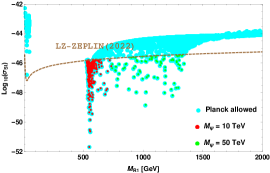
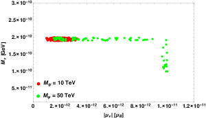
Figure 4: Left panel depicts the SI DM-nucleon cross section for the data (cyan) that satisfies Planck limit on relic density. Horizontal dashed line corresponds to LUX-ZEPLIN bound Aalbers et al. (2022). Various colored data points of red and green satisfy neutrino magnetic moment and mass for specific set of values for $M_{\psi}$, shown in the right panel.

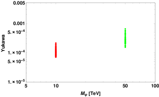
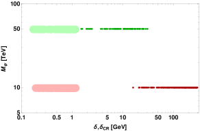
Figure 5: Allowed region of Yukawa for two set of values for $M_{\psi}$ in the left panel. Right panel provides the favourable region for mass splittings.

We first filter out the parameter space using the $3\sigma$ constraint on relic density. We then compute the DM-nucleon cross section and project it as a function of $M_{R1}$ in the left panel of Fig. 4. Here, all the cyan colored data points satisfy Planck satellite data Aghanim et al. (2018) in $3\sigma$ region and the parameter space (red and green) below LZ-ZEPLIN bound Aalbers et al. (2022) (orange dashed line) can satisfy neutrino magnetic moment and mass in the desired range when suitable values are assigned to Yukawa and vector-like lepton mass. The obtained neutrino observables are projected in the right panel for various set of values for $M_{\psi}$. The favorable range for Yukawa is displayed in the left panel of Fig. 5. Right panel depicts the allowed range for mass splittings.

Table 2: Set of benchmarks from the consistent parameter space.

	$M_{R1}$ [GeV]	$\delta$ [GeV]	$\delta_{\rm CR}$ [GeV]	$M_{\psi}$ [TeV]	Yukawa	$\sin\theta_{R}$	$\sin\theta_{C}$
benchmark-1	$975$	$13.68$	$0.62$	$50$	$10^{-3.58}$	$0.293$	$0.979$
benchmark-2	$798$	$26.12$	$0.88$	$50$	$10^{-3.75}$	$0.253$	$0.984$

Table 3: Neutrino and dark matter observables for the given benchmarks.

	$|\mu_{\nu}|\times 10^{12}$ [$\mu_{B}$]	$\mathcal{M}_{\nu}\times 10^{10}$ [GeV]	${\rm Log}^{[\sigma_{\rm SI}]}_{10}$ ${\rm cm}^{-2}$	$\Omega{\rm h}^{2}$
benchmark-1	$6.803$	$1.99$	$-46.58$	$0.12$
benchmark-2	$9.74$	$1.32$	$-46.05$	$0.122$

For two specific benchmark values (table. 2 and table. 3) that satisfies both neutrino and dark matter sectors, we project relic density as a function of lightest dark matter mass in Fig. 6.

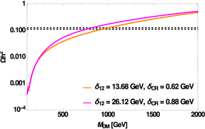
Figure 6: Relic density as a function of dark matter mass with horizontal dashed lines corresponding to Planck bound Aghanim et al. (2018).

VI.1 $\nu$MM implications on XENONnT

Recently XENONnT Aprile et al. (2022) has released a new data with upgraded detector and a total exposure of $1.16$ ton-years and reduced systematic uncertainties. With new upgrade, more than 50$\%$ of background reduction has been achieved and unlike its predecessor XENON1T, no excess events were reported in $1-7$ keV energy range of electron recoil. In this paper, we use XENONnT data to derive model independent limits on transition and effective magnetic moments by examining the changes in the $\nu-e^{-}$ elastic scattering cross section at low energies. We use non-maximal $\theta_{23}$ mixing to distinguish between the muon and tau neutrino interactions. We consider XENONnT background without solar contribution and then add the expected events due to new physics such as neutrino magnetic moment. In the presence of magnetic moment, the total differential cross section of $\nu-e^{-}$ scattering can be written as Giunti et al. (2016)

$$\left(\frac{d\sigma}{dT_{r}}\right)_{\rm TOT}=\left(\frac{d\sigma}{dT_{r}}\right)_{\rm SM}+\left(\frac{d\sigma}{dT_{r}}\right)_{\rm EM},$$ (23)

where, $T_{r}$ is the electron recoil energy. The first contribution in eq. 23 is due to standard weak interactions, given by

$$\left(\frac{d\sigma}{dT_{r}}\right)_{\rm SM}=\frac{G_{F}^{2}m_{e}}{2\pi}\left[(g_{V}+g_{A})^{2}+\left(1-\frac{T_{r}}{E_{\nu}}\right)^{2}(g_{V}-g_{A})^{2}+\left(\frac{m_{e}T_{r}}{E_{\nu}^{2}}\right)(g^{2}_{A}-g^{2}_{V})\right].$$ (24)

Here, $G_{F}$ stands for the Fermi constant, $E_{\nu}$ is the neutrino energy. $g_{V}$ and $g_{A}$ are the vector and axial vector couplings, which can be expressed in terms of weak mixing angle $\theta_{W}$ as

$$g_{V}=2\sin^{2}\theta_{W}+\frac{1}{2},~{}~{}~{}g_{A}=1/2~{}~{}{\rm for}~{}~{}\nu_{e}\;,$$

$$g_{V}=2\sin^{2}\theta_{W}-\frac{1}{2},~{}~{}~{}g_{A}=-1/2~{}~{}{\rm for}~{}~{}\nu_{\mu},\nu_{\tau}\;.$$ (25)

The second contribution in (23) comes from the effective electromagnetic vertex of the neutrinos, i.e., magnetic moment contribution, which can be expressed as

$$\left(\frac{d\sigma}{dT_{r}}\right)_{\rm EM}=\frac{\pi\alpha^{2}}{m^{2}_{e}}\left(\frac{1}{T_{r}}-\frac{1}{E_{\nu}}\right)\left(\frac{\mu_{\nu_{\alpha\beta}}}{\mu_{B}}\right)^{2}.$$ (26)

In the above, $\alpha$ is the fine-structure constant and $\mu_{\nu_{\alpha\beta}}$ is the neutrino magnetic moment and $\mu_{B}$ stands for Bohr Magneton. The differential event rate to estimate the XENONnT signal is given by

$$\frac{dN}{dT_{\rm vis}} = n_{\rm e}\times\int^{E^{\rm max}_{\nu}}_{E^{\rm min}_{\nu}}dE_{\nu}\int_{T^{\rm min}_{r}}^{T^{\rm max}_{r}}dT_{r}\left(\frac{d\sigma^{\nu_{e}e}}{dT_{r}}\overline{P_{ee}}+\cos^{2}\theta_{23}\frac{d\sigma^{\nu_{\mu}e}}{dT_{r}}\overline{P_{e\mu}}+\sin^{2}\theta_{23}\frac{d\sigma^{\nu_{\tau}e}}{dT_{r}}\overline{P_{e\tau}}\right)$$ (27)

$$\times\frac{d\phi_{s}}{dE_{\nu}}\times\epsilon(T_{\rm vis})\times G(T_{r},T_{\rm vis})\;,$$

where, $T_{\rm vis}$ represents the visible electron recoil energy at the detector, $\epsilon(T_{\rm vis})$ is the detector efficiency Aprile et al. (2022) and $d\phi_{s}/dE_{\nu}$ is the solar neutrino flux Bahcall and Pena-Garay (2004). $G(T_{r},T_{\rm vis})$ represents the normalized Gaussian smearing function, which takes into account the limited energy resolution of the detector with resolution power $\sigma(T_{\rm vis})/T_{\rm vis}=0.0015+(0.3171/\sqrt{T_{\rm vis}~{}{\rm[keV]}})$. In the above, $\overline{P_{ee}}$ and $\overline{P_{e\mu/\tau}}$ are the length averaged neutrino disappearance and appearance oscillation probabilities in the presence of matter effect respectively, can be expressed as Khan (2023)

$$\overline{P_{ee}}=\sin^{4}\theta_{13}+\frac{1}{2}\cos^{4}\theta_{13}\left(1+\cos 2\theta^{m}_{12}\cos 2\theta_{12}\right),$$

$$\overline{P_{e\mu}}+\overline{P_{e\tau}}=1-\overline{P_{ee}}\;,$$ (28)

where, $\theta^{m}_{12}$ is the effective mixing angle in the presence of matter effect Lopes and Turck-Chièze (2013) and we take the mixing angles from NuFit-5.2 Esteban et al. (2020). In eqn. (27), the differential cross sections can be expressed as the sum of SM and magnetic moment contributions as follows

$$\frac{d\sigma^{\nu_{e}e}}{dT_{r}}=\left(\frac{d\sigma}{dT_{r}}\right)_{SM}+\left(\frac{d\sigma}{dT_{r}}\right)_{\mu_{\nu_{e\mu}}}+\left(\frac{d\sigma}{dT_{r}}\right)_{\mu_{\nu_{e\tau}}},$$

$$\frac{d\sigma^{\nu_{\mu}e}}{dT_{r}}=\left(\frac{d\sigma}{dT_{r}}\right)_{SM}+\left(\frac{d\sigma}{dT_{r}}\right)_{\mu_{\nu_{e\mu}}}+\left(\frac{d\sigma}{dT_{r}}\right)_{\mu_{\nu_{\mu\tau}}},$$

$$\frac{d\sigma^{\nu_{\tau}e}}{dT_{r}}=\left(\frac{d\sigma}{dT_{r}}\right)_{SM}+\left(\frac{d\sigma}{dT_{r}}\right)_{\mu_{\nu_{e\tau}}}+\left(\frac{d\sigma}{dT_{r}}\right)_{\mu_{\nu_{\mu\tau}}}.$$ (29)

The integration limits on $E_{\nu}$ goes from $\left(T_{r}+\sqrt{2m_{e}T_{r}+T^{2}_{r}}\right)/2$ to 420 keV (corresponding to the upper limit of pp-chain in Sun). The other limit $T_{r}$ describes the threshold of the detector, which runs from 1 keV to 140 keV (recoil energy of interest). We now estimate the neutrino transition magnetic moment using XENONnT data through the least-squared statistical method and define the following $\chi^{2}$ function,

$$\chi^{2} = \sum_{k=1}^{70}\left(\left[\left(\frac{dN}{dT_{\rm vis}}(1+\alpha)+B\right)^{\rm theory}_{k}-\left(\frac{dN}{dT_{\rm vis}}\right)^{\rm observed}_{k}\right]\Large{/}\sigma_{k}\right)^{2}+\left(\frac{\alpha}{\sigma_{\alpha}}\right)^{2}.$$ (30)

Here, the subscript $k$ represents the $k^{\rm th}$ bin of our theoretical prediction and observed events, $\sigma_{k}$ corresponds to the statistical uncertainty in each bin. We have considered the systematic error ($\sigma_{\alpha}$) to be around $10\%$ (reflected through the pull parameter $\alpha$), corresponding to the solar neutrino flux for our analysis. We also included the penalties for the uncertainties in mixing angles $\theta_{12}$, $\theta_{13}$ and $\theta_{23}$.

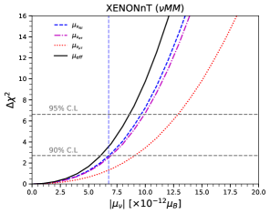
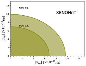
Figure 7: Left panel projects bounds on transition and effective magnetic moment, right panel shows the allowed region of transition magnetic moments in 90$\%$ and 95$\%$ C.L. for one degree of freedom at XENONnT experiment.

Left panel of Fig 7 shows the bounds on the neutrino transition magnetic moment and effective magnetic moment at 90$\%$ and 95$\%$ C.L. for the experiment XENONnT. The blue, violet and red curves represent the transition magnetic moment sensitivity of the components $\mu_{\nu_{e\mu}}$, $\mu_{\nu_{e\tau}}$ and $\mu_{\nu_{\mu\tau}}$ respectively, the black curve corresponds to the effective magnetic moment sensitivity of XENONnT experiment. The two grey horizontal lines stand for the sensitivity at 90$\%$ and 95$\%$ C.L. and the blue vertical line indicates the sensitivity of the experiment to transition magnetic moment $\mu_{\nu_{e\mu}}$ at 90$\%$ C.L. All the bounds on transition magnetic moments and effective magnetic moment are listed in Table 4. As the Sun is the source of electron type of neutrinos, we notice that the bounds on transition magnetic moments $\mu_{\nu_{e\mu}}$ and $\mu_{\nu_{e\tau}}$ are more constrained than $\mu_{\nu_{\mu\tau}}$. The right panel of Fig 7 shows the allowed region of transition magnetic moments in $\mu_{\nu_{e\mu}}-\mu_{\nu_{e\tau}}$ plane at 90$\%$ and 95$\%$ C.L for the experiment XENONnT. Hence, we end the discussion by saying that our model successfully generates transition magnetic moments in the allowed region.

$|\mu_{\nu}|$ $[\times 10^{-12}\mu_{B}]$
XENONnT	90$\%$ C.L	95$\%$ C.L
$\mu_{\rm eff}$	$<$ 6.08	$<$ 8.6
$\mu_{\nu_{e\mu}}$	$<$ 6.77	$<$ 9.63
$\mu_{\nu_{e\tau}}$	$<$ 6.98	$<$ 9.94
$\mu_{\nu_{\mu\tau}}$	$<$ 9.04	$<$ 12.9

Table 4: Bound on neutrino magnetic moment at 90$\%$ and 95$\%$ C.L at XENONnT experiment.

VII Concluding remarks

The primary motive of this model is to provide a simplified framework to invoke neutrino magnetic magnetic moment along with dark matter. The trick is to realize neutrino electromagnetic vertex with dark matter running in the loop. Using vector-like fermion and scalar multiplets, we attain magnetic moment and mass for light neutrinos via Type-II radiative scenario. The scalar triplet components annihilate and co-annihilate through the Standard Model scalar and vector bosons to provide correct order of dark matter relic density in the Universe (consistent with Planck satellite) and also get recoiled from detector, giving spin-independent cross section which is sensitive to stringent upper limit (LZ-ZEPLIN). Both the neutrino and dark matter aspects are thoroughly discussed in a common model parameter space, illustrated with suitable plots and benchmark values. Using XENONnT data, we have put bounds on transition magnetic moments in a model independent way. Finally, we sign off by saying that the model stands simple but phenomenologically rich in providing a common platform to address neutrino properties (magnetic moment and mass) and also dark matter physics (relic density and direct detection).

References

• Agostini et al. (2017) M. Agostini et al. (Borexino), Phys. Rev. D 96, 091103 (2017), eprint 1707.09355.
• Liu et al. (2004) D. W. Liu et al. (Super-Kamiokande), Phys. Rev. Lett. 93, 021802 (2004), eprint hep-ex/0402015.
• Beda et al. (2012) A. G. Beda, V. B. Brudanin, V. G. Egorov, D. V. Medvedev, V. S. Pogosov, M. V. Shirchenko, and A. S. Starostin, Adv. High Energy Phys. 2012, 350150 (2012).
• Wong et al. (2007) H. T. Wong et al. (TEXONO), Phys. Rev. D 75, 012001 (2007), eprint hep-ex/0605006.
• Daraktchieva et al. (2003) Z. Daraktchieva et al. (MUNU), Phys. Lett. B 564, 190 (2003), eprint hep-ex/0304011.
• Ayala et al. (2014) A. Ayala, I. Domínguez, M. Giannotti, A. Mirizzi, and O. Straniero, Phys. Rev. Lett. 113, 191302 (2014), eprint 1406.6053.
• Viaux et al. (2013) N. Viaux, M. Catelan, P. B. Stetson, G. Raffelt, J. Redondo, A. A. R. Valcarce, and A. Weiss, Phys. Rev. Lett. 111, 231301 (2013), eprint 1311.1669.
• Alok et al. (2023) A. K. Alok, N. R. Singh Chundawat, and A. Mandal, Phys. Lett. B 839, 137791 (2023), eprint 2207.13034.
• Miller Bertolami et al. (2014) M. M. Miller Bertolami, B. E. Melendez, L. G. Althaus, and J. Isern, JCAP 10, 069 (2014), eprint 1406.7712.
• Córsico et al. (2014) A. H. Córsico, L. G. Althaus, M. M. Miller Bertolami, S. O. Kepler, and E. García-Berro, JCAP 08, 054 (2014), eprint 1406.6034.
• Li and Xu (2023) S.-P. Li and X.-J. Xu, JHEP 02, 085 (2023), eprint 2211.04669.
• Aprile et al. (2022) E. Aprile et al. (XENON), Phys. Rev. Lett. 129, 161805 (2022), eprint 2207.11330.
• Khan (2023) A. N. Khan, Phys. Lett. B 837, 137650 (2023), eprint 2208.02144.
• Aghanim et al. (2018) N. Aghanim et al. (Planck) (2018), eprint 1807.06209.
• Clowe et al. (2006) D. Clowe, M. Bradac, A. H. Gonzalez, M. Markevitch, S. W. Randall, C. Jones, and D. Zaritsky, Astrophys. J. Lett. 648, L109 (2006), eprint astro-ph/0608407.
• Murayama (2007) H. Murayama, in Les Houches Summer School - Session 86: Particle Physics and Cosmology: The Fabric of Spacetime (2007), eprint 0704.2276.
• Singirala et al. (2023) S. Singirala, D. K. Singha, and R. Mohanta (2023), eprint 2306.14801.
• Lu and Gu (2017) W.-B. Lu and P.-H. Gu, Nucl. Phys. B 924, 279 (2017), eprint 1611.02106.
• Chen et al. (2021) S.-L. Chen, A. Dutta Banik, and Z.-K. Liu, Nucl. Phys. B 966, 115394 (2021), eprint 2011.13551.
• Sahoo et al. (2021) S. Sahoo, S. Singirala, and R. Mohanta (2021), eprint 2112.04382.
• Cirelli et al. (2006) M. Cirelli, N. Fornengo, and A. Strumia, Nucl. Phys. B 753, 178 (2006), eprint hep-ph/0512090.
• Ma and Suematsu (2009) E. Ma and D. Suematsu, Mod. Phys. Lett. A 24, 583 (2009), eprint 0809.0942.
• Xing and Zhou (2011) Z.-z. Xing and S. Zhou, Neutrinos in particle physics, astronomy and cosmology (2011), ISBN 978-3-642-17559-6, 978-7-308-08024-8.
• Babu et al. (2020) K. S. Babu, S. Jana, and M. Lindner, JHEP 10, 040 (2020), eprint 2007.04291.
• Ellis et al. (2000) J. R. Ellis, A. Ferstl, and K. A. Olive, Phys. Lett. B 481, 304 (2000), eprint hep-ph/0001005.
• Semenov (1996) A. V. Semenov (1996), eprint hep-ph/9608488.
• Pukhov et al. (1999) A. Pukhov, E. Boos, M. Dubinin, V. Edneral, V. Ilyin, D. Kovalenko, A. Kryukov, V. Savrin, S. Shichanin, and A. Semenov (1999), eprint hep-ph/9908288.
• Belanger et al. (2007) G. Belanger, F. Boudjema, A. Pukhov, and A. Semenov, Comput. Phys. Commun. 176, 367 (2007), eprint hep-ph/0607059.
• Belanger et al. (2009) G. Belanger, F. Boudjema, A. Pukhov, and A. Semenov, Comput. Phys. Commun. 180, 747 (2009), eprint 0803.2360.
• Aalbers et al. (2022) J. Aalbers et al. (LZ) (2022), eprint 2207.03764.
• Giunti et al. (2016) C. Giunti, K. A. Kouzakov, Y.-F. Li, A. V. Lokhov, A. I. Studenikin, and S. Zhou, Annalen Phys. 528, 198 (2016), eprint 1506.05387.
• Bahcall and Pena-Garay (2004) J. N. Bahcall and C. Pena-Garay, New J. Phys. 6, 63 (2004), eprint hep-ph/0404061.
• Lopes and Turck-Chièze (2013) I. Lopes and S. Turck-Chièze, Astrophys. J. 765, 14 (2013), eprint 1302.2791.
• Esteban et al. (2020) I. Esteban, M. C. Gonzalez-Garcia, M. Maltoni, T. Schwetz, and A. Zhou, JHEP 09, 178 (2020), eprint 2007.14792.