Variational Autoencoding of Dental Point Clouds

Abstract

Digital dentistry has made significant advancements, yet numerous challenges remain. This paper introduces the FDI 16 dataset, an extensive collection of tooth meshes and point clouds. Additionally, we present a novel approach: Variational FoldingNet (VF-Net), a fully probabilistic variational autoencoder designed for point clouds. Notably, prior latent variable models for point clouds lack a one-to-one correspondence between input and output points. Instead, they rely on optimizing Chamfer distances, a metric that lacks a normalized distributional counterpart, rendering it unsuitable for probabilistic modeling. We replace the explicit minimization of Chamfer distances with a suitable encoder, increasing computational efficiency while simplifying the probabilistic extension. This allows for straightforward application in various tasks, including mesh generation, shape completion, and representation learning. Empirically, we provide evidence of lower reconstruction error in dental reconstruction and interpolation, showcasing state-of-the-art performance in dental sample generation while identifying valuable latent representations.

1 Introduction

Recent advancements and widespread adoption of intraoral scanners in dentistry have made micrometer-resolution 3D models readily available. Consequently, the demand for efficiently organizing these noisy scans has grown in parallel. To this end, we propose a variational autoencoder (Kingma & Welling, 2014; Rezende et al., 2014) for point clouds to identify continuous representations, aligning with the continuous change and degradation of teeth over time.

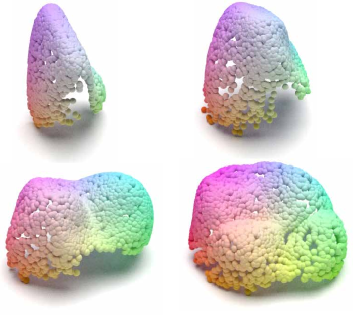
Figure 1: VF-Net samples, generated by our probabilistic variational autoencoder for point clouds.

Our solution is a probabilistic latent variable model that maintains a one-to-one point correspondence between points in the observed and generated point clouds. This one-to-one connection throughout the network allows for the optimization of the original variational autoencoder objective. We project the point cloud down to an intrinsic 2D surface representation to allow for efficient sampling and mitigate the storage of information regarding the overall shape in this space. These 2D projections impart a strong inductive bias, proving highly beneficial when the input point cloud and the 2D surface share topology. Simultaneously, creating a bottleneck prevents the model from learning the identity mapping. Specifically, our Variational Foldingnet (VF-Net) learns a projection of the 3D point cloud input down to 2D space, which then is deformed back into the input point cloud. Finally, these projections facilitate mesh generation without further training, as well as straightforward shape completion and shape extrapolation, all without compromising the quality of the learned representations (see Fig. 1 for samples).

Previous point cloud models generally lack one-to-one correspondence throughout the network due to their invariant architecture design. Instead, they evaluate reconstruction error using Chamfer distances ($\mathrm{CD}$) (Barrow et al., 1977) defined as

$$\begin{split}D(\mathbf{A}\rightarrow\mathbf{B})&=\frac{1}{|\mathbf{A}|}\sum_{\mathbf{a}\in\textbf{A}}\min_{\mathbf{b}\in\mathbf{B}}\|\mathbf{a}-\mathbf{b}\|_{2},\\ \textsc{Chamf-Dist}(\mathbf{C},\mathbf{D})&=D(\mathbf{C}\rightarrow\mathbf{D})+D(\mathbf{D}\rightarrow\mathbf{C}).\\ \end{split}$$ (1)

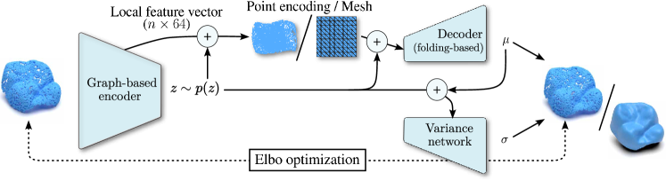
Figure 2: VF-Net is a variational autoencoder with a normalizing flow prior over the shape latent. Individual points are projected to 2D space, establishing a one-to-one connection and facilitating mesh generation and shape completion.

This metric solves the invariance problem. However, it also poses a new one: The Chamfer distance does not readily lead to a likelihood, preventing its use in probabilistic modeling. For instance, when used in the Gaussian distribution, the function $\mathbf{X}\mapsto\nicefrac{{1}}{{\mathcal{C}}}\exp(-\textsc{Chamf-Dist}^{2}(\mathbf{X},\mu))$ cannot be normalized to have unit integral due to the explicit minimization in Eq. 1. Consequently, previous latent variable models are closer to regularized autoencoders than the variational autoencoder. Since our model ensures one-to-one correspondence between points in the point clouds, we can easily build a proper probabilistic model.

Moreover, to encourage further research, we release a new dataset, the FDI 16 Tooth Dataset, which provides a large collection of dental scans, available as both meshes and point clouds. This dataset provides real-world representations with simple topologies. We consider this an excellent compromise between high-quality computer-aided design (CAD) models and sparse LiDAR scans (Chang et al., 2015, 2017; Caesar et al., 2020; Armeni et al., 2016). In digital dentistry, significant challenges are found in diagnostics, tooth (crown) generation, shape completion of obstructed areas of the teeth, and sorting point clouds.

In summary, we present the first fully probabilistic variational autoencoder for point clouds, VF-Net, characterized by a highly expressive decoder with state-of-the-art generative capabilities. All while learning compressed representations and being adaptable for shape completion tasks. Furthermore, we release a dataset of 7,732 tooth meshes to facilitate further research on real-world 3D data.

2 Related work

We focus on point cloud representations of 3D objects, but there are many alternative methods of representation including voxel grids (Zheng et al., 2021; Wu et al., 2018), multi-angle inference (Wen et al., 2019; Han et al., 2019), and meshes (Alldieck et al., 2019; Wang et al., 2018; Groueix et al., 2018). A major paradigm in neural networks for point clouds is to remain permutation and cardinality invariant. In terms of encoder-decoder models, this frequently leads to designs without a one-to-one correspondence between inputs and outputs (Yang et al., 2018; Groueix et al., 2018). This becomes an obstacle in adapting the variational autoencoder to point clouds. Accordingly, other methods have become prominent, including GANs (Li et al., 2018, 2019), diffusion models (Zhou et al., 2021; Zeng et al., 2022), and traditional autoencoders (Achlioptas et al., 2018; Groueix et al., 2018; Pang et al., 2021).

Existing Point Cloud Variational Autoencoders. One attempt to design a variational autoencoder for point clouds is SetVAE (Kim et al., 2021), which uses transformers to process sets of point clouds. Their primary novelty is introducing a latent space with an enforced prior inside the transformer block. These transformer blocks are then stacked to form a hierarchical variational autoencoder (Sønderby et al., 2016), posing issues in evaluating its representations. However, the SetVAE is not fully probabilistic as the reconstruction loss is approximated via Chamfer distances, resulting in a model closer to a regularized autoencoder than a variational autoencoder. LION (Zeng et al., 2022) is a latent variable model that maintains a one-to-one mapping throughout the network, allowing for probabilistic evaluation. However, they only implicitly utilize this by optimizing an L1-loss. Similar to our work, they also encode their points, but instead of bottlenecking this, they map them to a higher dimensional space. This, unfortunately, leads to information about the shape being stored here, preventing direct sampling/modification in this space. Finally, similarly to SetVAE, evaluating the quality of representations in LION, a hierarchical latent variable model, poses challenges. FrePolad (Zhou et al., 2023) is another latent diffusion model similar to LION. Their primary novelty is the introduction of the frequency rectification module that better captures high-frequency signals in point clouds. They train their model via a modified VAE loss to account for frequency rectified distances.

Other Generative Models. One fully probabilistic work is PointFlow (Yang et al., 2019). PointFlow uses a continuous normalizing flow (CNF) both as prior and decoder, similar to previous works seen on images (Kingma et al., 2017; Sadeghi et al., 2019). Intuitively, one CNF can be considered modeling the distribution of shapes, while the other models the point distribution given the shape. Similarly, VF-Net’s encoder maps a global latent space, and the point encoding projections offer a latent mapping for each input point. However, PointFlow’s two CNFs are trained separately, while in VF-Net, these are trained simultaneously. PointFlow is unfortunately very slow (Kim et al., 2021). On our full proprietary dataset, PointFlow would have required 200 GPU days of training. Thus, we excluded it from our baselines. Diffusion models such as diffusion probabilistic model (DPM) (Luo & Hu, 2021) and point-voxel diffusion (PVD) (Zhou et al., 2021) present two diffusion models for the point clouds, especially PVD generates excellent new samples. However, diffusion models do not find compressed structured representations of the data as our VF-Net does; see table. LABEL:tab:method_properties for a model property overview.

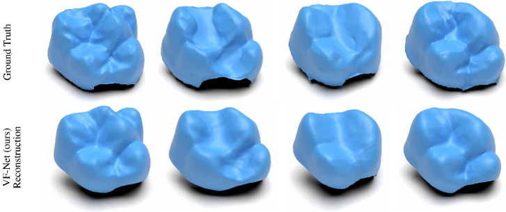
Figure 3: Top: Samples from the FDI 16 dataset with varying facet regularity and resolution. Bottom: VF-Net reconstructions.

Digital Dentistry. In computational dentistry, extrapolating the tooth’s obstructed sides is a well-known task. Qiu et al. (2013) presents an impressive attempt to use classic computational geometry methods. They attempt to reconstruct the missing parts of the distal and mesial sides of the tooth. This leads to a very smooth extrapolation, which performs well. Several works within dentistry take this a step further, e.g., attempting to extrapolate not just the sides but also the roots of the teeth (Wei et al., 2015; Zhou et al., 2018; Wu et al., 2016). Unfortunately, CBCT scans are expensive and rare; thus, we do not have a large enough dataset for neural network training.

3 Variational Point Cloud Inference

Background: FoldingNet. To handle varying sizes and arbitrary order in point clouds, a common strategy is to employ neural networks exhibiting invariance to changes in cardinality and permutation, as proposed by Qi et al. (2017) in PointNet. FoldingNet employs a very similar encoder, $e$, that operates independently on each point of the point cloud to identify the latent code, $\mathbf{z}$. Subsequently, the folding-based decoder, $f:\mathcal{Z}\times\mathbb{R}^{2}\rightarrow\mathbb{R}^{3}$, "folds" a chosen constant base shape, $\mathcal{G}$, according to the latent code, in our case two-dimensional planar patch $[-1,1]^{2}$ (Yang et al., 2018). Both the encoder, $e$, and the decoder, $f$, are jointly trained to minimize the reconstruction error approximated via Chamfer distances (1),

$$\mathcal{E} =\textsc{Chamf-Dist}\left(\mathbf{x}-f(e(\mathbf{x}),\mathcal{G})\right).$$ (2)

This ensures invariance to cardinality and permutation changes, although it complicates variational inference extensions. A variational autoencoder yields a distribution for each input (Kingma & Welling, 2014; Rezende et al., 2014). However, FoldingNet and most current permutation-invariant neural networks do not have a correspondent output point for each input point in the point cloud.

3.1 The Variational FoldingNet

Following the variational autoencoder architecture, Variational FoldingNet introduces a prior to the latent space. Our aim is to instill greater structure to identify more robust representations. This also facilitates improved handling of missing and noisy data, which is important for real-world datasets. Motivated by unsupervised probabilistic representation learning’s benefits across many tasks, including generative modeling (Kingma & Welling, 2014; Rezende et al., 2014; Dinh et al., 2017; Ho et al., 2020), out-of-distribution detection (Nalisnick et al., 2019; Havtorn et al., 2021), handling missing data (Mattei & Frellsen, 2019) etc, we introduce Variational FoldingNet (VF-Net). For a complete architecture overview, consult Fig. 2.

One key feature is the introduction of a novel projection down to the planer space, $[-1,1]^{2}$, $\mathrm{proj}_{\mathcal{G}}(\mathbf{x}):\mathbb{R}^{3}\rightarrow\mathcal{G}$, where $\mathbf{g}\in\mathcal{G}$. Note that no prior is placed upon the projections, which we will refer to as our point encodings. We establish a one-to-one correspondence throughout the entire network by decoding these point encodings instead of a constant planar patch. However, it also follows that the projected points, $\hat{\mathcal{G}}$, are no longer constant or independent of input $\mathbf{x}$. The folding of $\hat{\mathcal{G}}$ from the planar space, $f(\hat{\mathcal{G}})$, remains determined by the parameter vector $\mathbf{z}$ predicted by the PointNet encoder, $e$. This projection is learned together with the rest of the model,

$$S =f(\mathbf{z},\hat{\mathcal{G}}(\mathbf{x},\mathbf{z}))$$ (3)

$$\hat{\mathcal{G}}(\mathbf{x},\mathbf{z}) =\operatorname*{arg\,min}_{\hat{\mathbf{g}}\in\hat{\mathcal{G}}}\|\mathbf{x}-f(\mathbf{z},\hat{\mathbf{g}})\|^{2}.$$ (4)

$S$ is the surface spanned by $f(\mathbf{z},\mathcal{\hat{G}})$. This is a permutation invariant and cardinality invariant autoencoder with a one-to-one point correspondence from end to end. This enables optimization through traditional variational autoencoder methods.

To facilitate variational extension, we define the likelihood of the observed data as $p(\mathbf{x})=\int p(\mathbf{x}|\mathbf{z})p(\mathbf{z})\mathrm{d}\mathbf{z}$, which gives a training objective. Unfortunately, the integral is generally intractable, and approximations are necessary. Following conventional variational inference (Kingma & Welling, 2014; Rezende et al., 2014), a lower bound (Elbo) on $p(\mathbf{x})$

Table 2: Across five seeds, VF-Net produces close to as large a variety of teeth as PVD and LION while generating samples much closer to real teeth. MMD has been multiplied by 100.

Method	MMD($\downarrow$)		COV(%$\uparrow)$		1-NNA(%$\downarrow)$
	CD	EMD	CD	EMD	CD	EMD
Train subsampled	21.00$\pm$0.09	51.53$\pm$0.06	49.00$\pm$0.64	46.95$\pm$2.79	49.83$\pm$0.68	50.97$\pm$0.82
SetVAE	39.00$\pm$0.78	66.66$\pm$0.38	10.66$\pm$0.66	9.52$\pm$0.27	97.99$\pm$0.32	97.95$\pm$0.34
DPM	20.71 $\pm$0.10	51.94$\pm$0.09	36.94$\pm$0.65	33.28$\pm$0.65	70.30$\pm$0.82	75.75$\pm$0.99
PVD	21.58$\pm$0.03	51.64$\pm$0.08	44.11$\pm$0.76	43.23$\pm$0.92	62.85$\pm$0.78	60.70$\pm$1.06
LION	22.12$\pm$0.15	52.75$\pm$0.12	45.12$\pm$0.60	43.32$\pm$1.28	68.56$\pm$0.73	66.76$\pm$0.94
VF-Net (Ours)	20.38$\pm$0.09	49.72$\pm$0.04	42.85$\pm$0.64	40.20$\pm$0.71	56.31$\pm$0.39	56.05$\pm$0.32

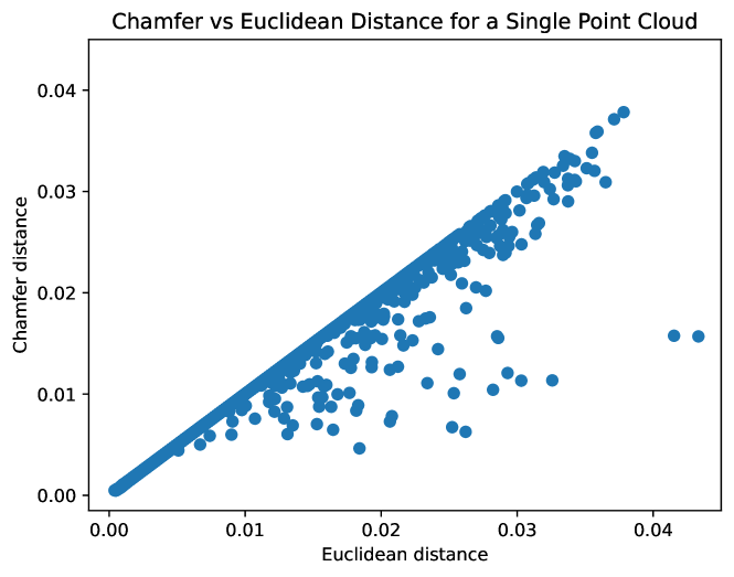
Figure S1: In the depicted plot, it is evident that the Euclidean distance serves as an upper limit for the Chamfer distance. In most instances, optimization with VF-Net results in nearly identical distances. This empirical finding supports our claim that the Chamfer distance can be efficiently replaced with an appropriate encoder choice.

where $q(\mathbf{z}|\mathbf{x})$ is an approximation to the posterior $p(\mathbf{z}|\mathbf{x})$. Most current point cloud models replace the likelihood with a distance metric here, making the models closer to a regularized autoencoder. Our novel method for probabilistic evaluation for 3D reconstruction networks avoids the computationally expensive Chamfer distance, Eq. 1. In supplementary Fig. S1, we demonstrate that our projections can effectively replace Chamfer distances. The two metrics closely align, with Euclidean distances acting as an upper bound that tightens with improved reconstruction precision. Other permutation invariant networks lack this one-to-one connection between input and output, making such evaluation impossible. Instead, they rely on Chamfer distances (1) (Yang et al., 2018; Groueix et al., 2018; Kim et al., 2021), but no suitable normalization constant can be derived for probabilistic distributions using Chamfer distances. Consequently, probabilistic evaluation using Chamfer distances is impossible.

During the evaluation of the Elbo loss, we use a multivariate student-t distribution with isotropic variance and three degrees of freedom as the reconstruction term. This choice helps to decrease emphasis on outliers and instead focus more on the majority of the data points. $p(x|\mathbf{z},\mathbf{g})=\text{Student-t}(x|f(\mathbf{z},\mathbf{g}),\sigma^{2}(\mathbf{z},\mathbf{g})\mathbf{I},\nu)$, where $f:\mathcal{Z}\times\mathbb{R}^{2}\rightarrow\mathbb{R}^{3}$ and $\sigma^{2}:\mathcal{Z}\times\mathbb{R}^{2}\rightarrow\mathbb{R}_{+}$ are neural networks. No major changes were made to the generative process. We let $p(\mathbf{z})$ be a normalizing flow prior over the parameters describing the shape of an object (Kingma et al., 2017). When the input, $\mathbf{X}$, and the projections, $\mathcal{G}$, share topology, the bias allows for uniform sampling in the planar patch $[-1,1]^{2}$. As in FoldingNet, this grid is subsequently deformed according to $\mathbf{z}$. New samples can thus be generated by first sampling $\mathbf{z}$ and then mapping the uniformly sampled grid points through $f$ and $\sigma$,

$$\mathbf{x}=f(\mathbf{z},\mathbf{g})+\sigma(\mathbf{z},\mathbf{g})\cdot\mathbf{t},\quad\mathbf{t}\sim\text{Student-t}(\mathbf{\nu}).$$ (6)

This also enables straightforward mesh generation as deformations are smooth - points projected closely to each other correspond to points close in output space. Consequently, we can generate meshes by simply defining the facets in the 2D planar space.

4 The FDI 16 Tooth Dataset

To improve the state-of-the-art modeling of dental scans, we will release an extensive new dataset alongside this paper. The FDI 16 dataset is a collection of 7,732 irregular triangle meshes of the right-side first maxillary molar tooth formally denoted as ’FDI 16’ following ISO 3950 notation (see Fig. 3). These meshes were acquired from fully anonymized intraoral scans primarily scanned using 3Shape’s TRIOS 3 scanners. Each tooth in the FDI 16 Tooth dataset was algorithmically segmented from an upper jaw scan by 3Shape’s Ortho Systems 2023. As the teeth are a subsection of a full intraoral jaw scan, there will be areas obstructed by the adjacent teeth. The teeth, therefore, constitute open meshes and have clear boundaries with no representation of interior object volume. All tooth meshes are from patients undergoing aligner treatment, and accordingly, aligner attachments will be present in a substantial number of scans. This introduces a bias towards younger individuals, who generally have fewer restorations and dental problems. The top row of Fig. 3 shows examples of such meshes. All scans have been made publicly available fully anonymously as meshes and point clouds at millimeter scale. The teeth have been algorithmically rotated to ensure that the $x$-axis is turned towards the neighboring tooth (FDI 17) while the $y$-axis points in the occlusal direction (direction of the biting surface). Finally, the $z$-axis is given by the cross-product to ensure a right-hand coordinate system.

Dental scans have a diverse set of research applications. This study explores reconstruction, generation of new teeth, representation learning, and shape completion. All of which have different but critical applications in digital dentistry. We believe that the FDI 16 dataset addresses a crucial niche within 3D datasets by offering a dataset that strikes a balance between the highly detailed but idealized CAD scans (Chang et al., 2015) and sparser real-world LIDAR scans (Chang et al., 2017; Caesar et al., 2020; Armeni et al., 2016). This dataset provides a valuable middle ground. Note that any method considered for deployment must be capable of running efficiently on edge devices without a significant performance overhead. This is particularly important as intraoral scanners must function seamlessly even in areas with limited network connectivity.

5 Experimental results

We next evaluate VF-Net’s performance on point cloud generation, auto-encoding, shape completion, and unsupervised representation learning. Note that FrePolad (Zhou et al., 2023) has been excluded from comparison as no public implementation is available.

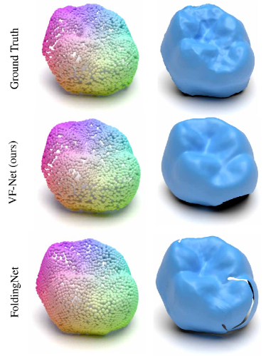
Figure 4: FoldingNet’s mesh reconstructions have gaps and highly distorted facets. Conversely, VF-Net’s mesh facets are even more regular than the input point cloud, and points in the reconstruction are placed closely resembling its input.

Point cloud generation. To compare sampling performances, we deploy three established metrics for 3D generative model evaluation (Yang et al., 2019). Namely, minimum matching distance (MMD) is a metric that measures the average distance to its nearest neighbor point cloud. Coverage (COV) measures the fraction of point clouds in the ground truth test set that is considered the nearest test sample neighbor for a generated sample. 1-nearest neighbor accuracy (1-NNA) uses a 1-NN classifier to classify whether a sample is generated or from the ground truth dataset, 50%, meaning generated samples are indistinguishable from the test set. Data handling and training details for FDI 16 experiments can be found in supplementary section S1.3 and S1.4, respectively.

Table 3: Chamfer distances (CD) and earth mover’s distances (EMD) are multiplied by 100.

Method	FDI 16 Tooth		All FDIs
	$\mathbf{CD}$	$\mathbf{EMD}$	$\mathbf{CD}$	$\mathbf{EMD}$
DPM	10.04	43.98	5.67	35.8
SetVAE	21.50	59.24	9.98	51.48
LION	5.35	22.85	3.02	9.66
FoldingNet	5.26	33.67	3.43	31.25
VF-Net (ours)	1.21	6.30	0.97	5.30

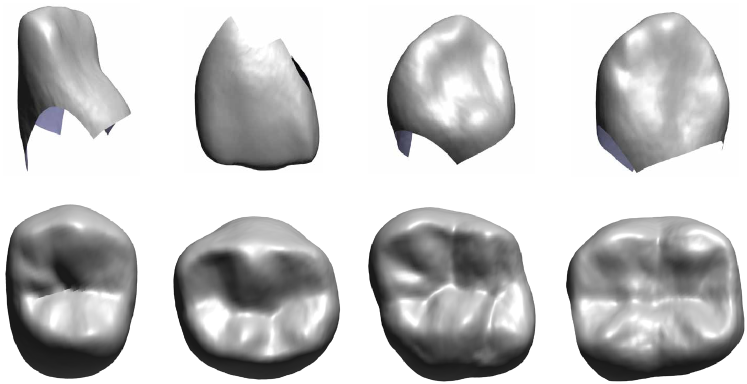
Figure S2: A display of meshes sampled by VF-Net showcases comprehensive coverage across the four major tooth modalities: Incisor, canine, pre-molar, and molar. These represent the primary types of teeth in the proprietary dataset.

Sampling from VF-Net can be done by sampling a uniform grid in the latent point encodings space, akin to FoldingNet. However, the corners of the uniform grid cause edge artifacts in the generated samples, evident in generated meshes in Fig. S2. The sampling metrics heavily punish such artifacts. Instead, we trained a minor network similar to the decoder of FoldingNet to predict the point encodings from the latent representation. We emphasize that this is entirely unnecessary for regular sampling. The sampling evaluations across five different seeds can be found in Table 2. The results demonstrate that VF-Net generates much more accurate samples, as evidenced by the significantly lower MMD and 1-NNA scores while being close in diversity to PVD and LION (Zhou et al., 2021; Zeng et al., 2022). Furthermore, sampling is much faster than PVD and LION as VF-Net does not depend on an iterative diffusion process. Note that while MMD is very stable across seeds, the COV and 1-NNA scores may vary quite a bit.

Outside of the FDI 16 dataset, we also train VF-Net on a proprietary dataset, which includes the remaining teeth from the FDI 16 jaws; see supplementary section S1.5 for training details. However, we did not quantify sampling performance, as sampling evaluation on 40k test samples would be exceedingly computationally expensive. We observe that VF-Net can sample from all major teeth types, incisors, canines, premolars, and molars, see Fig. 1. Additional mesh samples may be found in supplementary Fig. S2.

Point cloud auto-encoding. We evaluate VF-Net’s reconstruction quality to the previously mentioned generative models and FoldingNet. This evaluation was performed on both on FDI 16 dataset and the larger proprietary dataset. Please consult supplementary sections S1.3 and S1.5 for data handling and training details. We evaluated reconstructions using Chamfer distance and earth mover’s distance (Rubner et al., 2000),

$$\vspace{-2pt}\operatorname{EMD}(\mathbf{X},\mathbf{Y})=\min_{\phi:\mathbf{X}\rightarrow\mathbf{Y}}\sum_{\mathbf{x}\in\mathbf{X}}\|\mathbf{x}-\phi(\mathbf{x})\|_{2}.\vspace{-2pt}$$ (7)

The earth mover’s distance measures the least expensive one-to-one transportation between two distributions. However, this is computationally expensive and thus rarely used for model optimization (Wu et al., 2021). The reconstruction errors are presented in Table 3. Point-Voxel Diffusion (PVD) (Zhou et al., 2021) was excluded from comparison due to not returning the same tooth upon reconstruction.

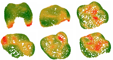
Figure 5: Intra-point cloud relative predicted variance (red is high, green is low). Notably, the carabelli cusp and aligner attachment areas exhibit high variance, two features only present in a subset of individuals.

VF-Net achieves a significantly lower reconstruction error than our comparison methods on both the FDI 16 dataset and the proprietary dataset comprising 119,496 teeth, encompassing 32 distinct teeth. As shown in Fig. 4, VF-Net’s one-to-one correspondence is evident in its reconstruction. The point placements mimic those in the input point cloud, while FoldingNet’s points are evenly distributed. VF-Net and FoldingNet can both generate meshes without any additional training of the model. In Fig. 4, deformation artifacts from FoldingNet that were not as visible from its point cloud are evident. FoldingNet folds the edge across the tooth to accommodate teeth of different sizes. Besides mesh gaps, this also leads to highly irregular facets that intersect one another. On the other hand, VF-Net can adjust the point encoding area to avoid such artifacts. However, VF-Net’s reconstructions often exhibit excessive smoothness and lack the desired level of detail. A common observation in variational autoencoders (Kingma & Welling, 2014; Vahdat & Kautz, 2021; Tolstikhin et al., 2019).

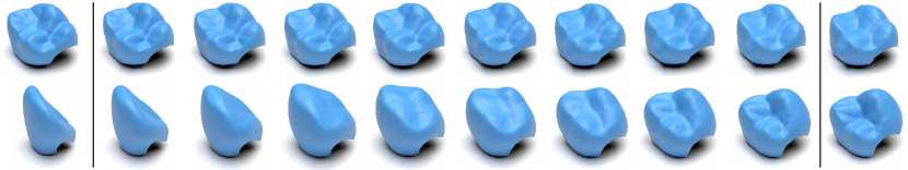
Figure 7: Interpolating between two teeth by interpolating their latent codes using the same mesh decoding.

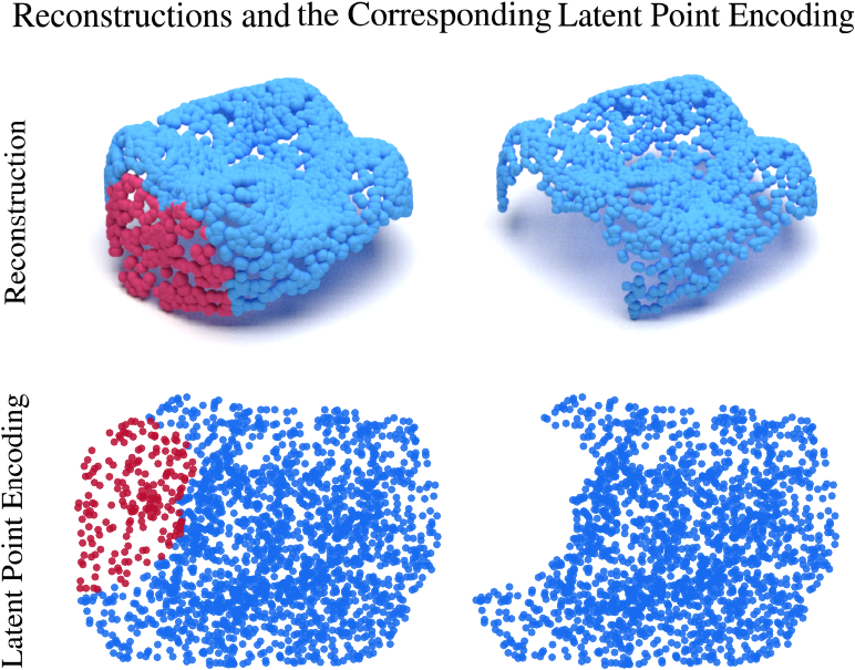
Figure 6: Left: Red points are removed from the point cloud. Right: Reconstruction and projected point encodings remain highly similar despite point deletion. Sampling the missing area is facilitated by sampling within the corresponding empty region of the latent point encoding.

Variance estimation for point clouds. Predicted variances from the variance network are shown in Fig. 5, where red indicates a higher variance and green indicates a lower variance within each point cloud. Interestingly, the network assigns higher variance to the fifth cusp and aligner attachments, features only present in a subset of samples. Furthermore, the border of the mesh tends to be assigned higher variance, likely due to a combination of data loading and segmentation artifacts. When the network is not in doubt about the previously mentioned two factors, the network assigns the highest variance to the occlusal surface. All of which aligns with expectations of areas of the teeth that have the most variance.

Simulated shape completion. One significant benefit of the inductive bias from the point encodings is straightforward shape completion and shape extrapolation. In computational dentistry, inferring the obstructed sides of a tooth and reconstructing the tooth surface beneath obstructions such as braces pose a key challenge. Paired data of obstructed and unobstructed surfaces is exceedingly rare. Therefore, developing a model capable of extrapolating such surfaces without explicit training is highly desirable. To this end, we simulate the task by evaluating the interpolation performance of each model. This is done by sampling a point on the outward side of the tooth and deleting its nearest neighbors to a total of 200 points. Selecting a mid-buccal point simulates bracket removal prediction ("Bracket sim") while opting for a lower buccal point simulates the obstructed side prediction ("Gap sim").

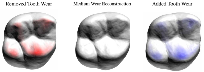
Figure 8: Moving toward tooth wear in the latent space. Left: Highlighted in red are areas with higher values than the original reconstruction. Middle: The original reconstruction. Right: Areas depicted in blue are lower than the original mesh. In general, as the level of tooth wear increases, we observe a gradual smoothing in the occlusal surface.

An example of a synthetic hole is depicted in Fig. 6, where the red points are to be removed. Both reconstructions and latent point encodings remain highly similar despite the removal of the red points. Extrapolation/interpolation can be performed by sampling in the point encoding space. To quantify the interpolation performance, we calculate the distance from the deleted points to their nearest neighbor in the completed point cloud; see supplementary Sec. S1.7 for more experiment details. To contextualize the performance, we trained several shape completion methods (PVD (Zhou et al., 2021), PoinTr (Yu et al., 2021), VRCNet (Pan et al., 2021)). Since these methods only predict the missing area, a completely fair comparison cannot be made. The results can be found in Table 4, under "Bracket sim" and "Gap sim," simulating the removed bracket and the gap between teeth, respectively. Here, VF-Net outperforms its peers when it comes to untrained interpolation, and as expected there is a gap in performance between the trained and untrained methods. Shape completion using LION’s latent points from the original tooth contains information about the shape, rendering a fair comparison infeasible.

Table 4: Unsupervised generative models in the top half are untrained interpolation, while the bottom half are trained models. All Chamfer distances have been multiplied by 100.

	Method	Bracket sim	Gap sim
Unsupervised	DPM	15.88	38.00
	SetVAE	11.50	13.35
	FoldingNet	16.42	20.14
	VF-Net (ours)	4.35	3.55
Supervised	PVD	2.23	2.37
	PoinTr	1.84	1.83
	VRCNet	2.42	2.04

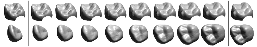
Figure S3: Interpolating between two teeth by interpolating their latent codes using the same mesh decoding.

Representation learning. We compare our latent representation to FoldingNet’s, as it is the comparison model with the most interpretable latent variables. First, we follow FoldingNet’s proposed evaluation method of classifying the input point cloud from the latent space. Using a linear support vector machine (SVM) to classify which tooth from the larger proprietary dataset is embedded, a 32-class problem. Here, the SVM achieves 96.80% accuracy on VF-Net’s latent codes compared to 96.36% of FoldingNet. Indicating all global point cloud information is stored in the latent variables, meaning the latent point encodings exclusively contain information about specific points. No information pertaining to the overall point cloud shape is stored in the point encodings. For qualitative assessment, an interpolation between two FDI 16 teeth and an interpolation example between an incisor and a premolar can be found in Fig. 7. Both interpolations exhibit a seamless transition in the latent space; for a more detailed view, see supplementary Fig. S3.

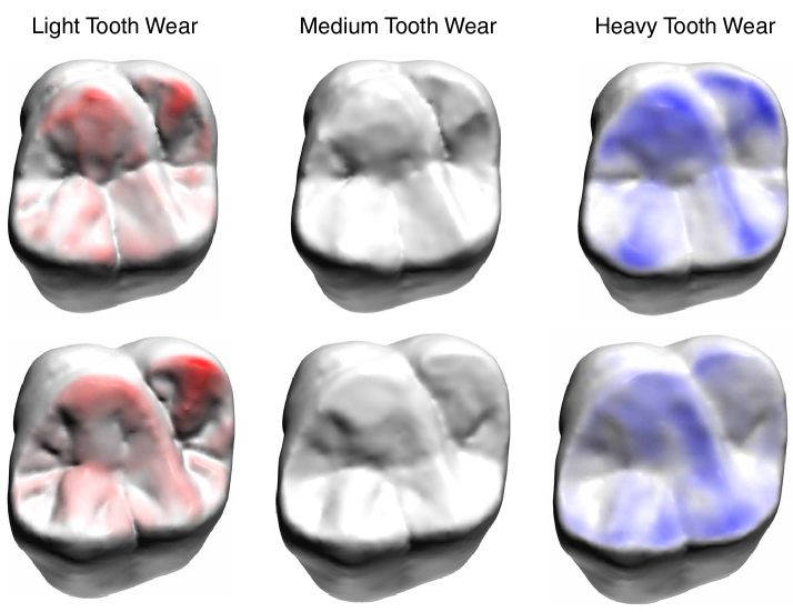
Figure S4: Two of the ten manually sculpted teeth to simulate tooth wear. Left: Areas with higher values compared to the original mesh are highlighted in red. Middle: The original mesh. Right: The mesh showcases areas depicted in blue that are lower than the original mesh.

Next, we attempt to add and remove toothwear; see Fig. 8. We navigate the latent space of VF-Net in the direction of tooth wear or away from it. The direction was determined by calculating the average change in latent representations when encoding 10 teeth from their counterparts with synthetically induced tooth wear. These teeth were manually sculpted to simulate tooth wear; see supplementary Fig. S4. We observe behavior that closely aligns with our expectations of how the tooth would change when adding or subtracting tooth wear.

To quantify the performance, we train a small PointNet model (Qi et al., 2017) on a proprietary dataset of 1400 teeth annotated with light/medium/heavy tooth wear. Subsequently, validate whether a change in the latent space yielded the expected change in classifier prediction. In Table 5, each class denotes the base class before adding/removing tooth wear. For light and heavy, we added and removed tooth wear, respectively, while medium tooth wear teeth were evaluated both when adding/removing wear. The findings presented in Table 5 indicate that VF-Net’s latent representations show greater robustness.

Table 5: The percentage of teeth with the expected change in classification prediction when changing the latent code towards/away from the tooth wear direction. L, M, and H denote light, medium, and heavy wear.

Method	L	M	H
FoldingNet	94.95%	91.77%	97.8%
VF-Net (ours)	97.98%	96.31%	98.68%

Limitations. Until now, the inductive bias from folding a 2D plane to a point cloud has proven highly beneficial. This is only the case when the input point cloud shares topology with the 2D plane. Unfortunately, this inductive bias is not as beneficial when the two topologies differ. We trained VF-Net on ShapeNet data (Chang et al., 2015). The drawback is not evident through the reconstructions; see supplementary Table S1. VF-Net has a low reconstruction error, but LION boasts the lowest. Issues arise when attempting to generate new samples. Due to information of the shape being stored in the latent point encodings, as depicted in Fig. 9. The latent point encodings form a non-continuous distribution, posing challenges for sampling new models. Note that for point clouds sharing topology, VF-Net is strongly biased towards generating a continuous distribution; see Fig. 9. Addressing this issue could involve training a flow or diffusion prior for the point encodings, similar to the approach used in LION (Zeng et al., 2022). However, since this was not the focus of our model, we did not pursue this idea.

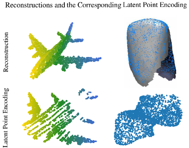
Figure 9: Left: While accurately reconstructed, the airplane forms a non-continuous distribution in the latent point encoding, posing challenges for sampling. Right: An incisor and its corresponding point encodings.

6 Conclusion

We have introduced the FDI 16 dataset and Variational FoldingNet (VF-Net), a fully probabilistic point cloud model in the same spirit as the original variational autoencoder (Kingma & Welling, 2014; Rezende et al., 2014). The key technical innovation is the introduction of a point-wise encoder network that replaces the commonly used Chamfer distance, allowing for probabilistic modeling. Importantly, we have shown that VF-Net offers better auto-encoding than current state-of-the-art generative models and more realistic sample generation for dental point clouds. Additionally, VF-Net offers straightforward shape completion and extrapolation due to its latent point encodings. All while identifying highly interpretable latent representations.

Appendix S1 Supplementary Material

S1.1 Chamfer vs Euclidean

S1.2 ShapeNet Reconstruction Performances

Table S1: Both Chamfer distances (CD) and earth mover’s distances (EMD) are multiplied by 1000. Lower values indicate better reconstruction performance.

Method	ShapeNet Airplanes
	$\mathbf{CD}$	$\mathbf{EMD}$
DPM	0.18	47.82
SetVAE	0.14	30.60
PVD	0.31	90.45
LION	0.025	7.30
FoldingNet	0.079	31.47
VF-Net (ours)	0.039	7.90

S1.3 Data Handling

For dental scan experiments, the point clouds used were constructed from vertices and facet midpoints. The cardinality of the raw point clouds varied significantly, ranging from around 2,000 to 65,000 points. To handle this, we subsampled 2048 points from each point cloud during training. As FoldingNet and VF-Net deform from a set space, selecting an appropriate normalization method is crucial. The normalization determines the amount of deformation needed for initial points to reach the desired final reconstruction. As we have defined our planar patch as $[-1,1]^{2}$, we scale the data so 99.5%

S1.4 FDI 16 Training Details

VF-Net was trained using an Adamax optimizer with an initial learning rate of 0.001. Each backpropagation iteration utilized a batch size of 64, and the training persisted for 16,000 epochs. We employed a KLD warm-up (Sønderby et al., 2016) during the initial 4,000 epochs, whenever applicable. During the initial training of VF-Net, a constant variance was used. Following that, a distinct training phase of 100 epochs was explicitly conducted to train the variance network.(Detlefsen et al., 2019).

S1.5 All FDI Training Details

In the experiments conducted on the proprietary dataset, encompassing all teeth, each model maintained the same architecture and size as employed in the FDI 16 experiment. However, training was confined to 1,250 epochs, incorporating a KLD warm-up phase constituting one-fourth of the total epochs when relevant. Again, a separate training run of 100 epochs was done to tune the variance network (Detlefsen et al., 2019).

S1.6 Sampled All FDI Teeth

S1.7 Shape Completion Experiments

In the shape completion experiments, each model is permitted to sample three times the standard number of points. Unsupervised models, therefore, have the allowance to sample 6,144 points each, as their sampling is not limited to the missing area. Conversely, for supervised models trained to predict the 200 missing points, we extract 600 points in this region to balance point density between supervised and unsupervised models. The evaluation is done by calculating a one-directional Chamfer distance (1) from predicted points to ground truth, quantifying shape completion performance.

S1.8 Interpolation

S1.9 Synthetic Toothwear Teeth

References

- Achlioptas et al. (2018) Achlioptas, P., Diamanti, O., Mitliagkas, I., and Guibas, L. Learning Representations and Generative Models for 3D Point Clouds, June 2018. URL http://arxiv.org/abs/1707.02392. arXiv:1707.02392 [cs].
- Alldieck et al. (2019) Alldieck, T., Pons-Moll, G., Theobalt, C., and Magnor, M. Tex2Shape: Detailed Full Human Body Geometry From a Single Image. arXiv:1904.08645 [cs], September 2019. URL http://arxiv.org/abs/1904.08645. arXiv: 1904.08645.
- Armeni et al. (2016) Armeni, I., Sener, O., Zamir, A. R., Jiang, H., Brilakis, I., Fischer, M., and Savarese, S. 3D Semantic Parsing of Large-Scale Indoor Spaces. In 2016 IEEE Conference on Computer Vision and Pattern Recognition (CVPR), pp. 1534–1543, Las Vegas, NV, USA, June 2016. IEEE. ISBN 978-1-4673-8851-1. doi: 10.1109/CVPR.2016.170. URL http://ieeexplore.ieee.org/document/7780539/.
- Barrow et al. (1977) Barrow, H. G., Tenenbaum, J. M., Bolles, R. C., and Wolf, H. C. Parametric Correspondence and Chamfer Matching: Two New Techniques for Image Matching. August 1977. URL https://openreview.net/forum?id=rkb6wXfdWB.
- Caesar et al. (2020) Caesar, H., Bankiti, V., Lang, A. H., Vora, S., Liong, V. E., Xu, Q., Krishnan, A., Pan, Y., Baldan, G., and Beijbom, O. nuScenes: A multimodal dataset for autonomous driving, May 2020. URL http://arxiv.org/abs/1903.11027. arXiv:1903.11027 [cs, stat].
- Chang et al. (2017) Chang, A., Dai, A., Funkhouser, T., Halber, M., Nießner, M., Savva, M., Song, S., Zeng, A., and Zhang, Y. Matterport3D: Learning from RGB-D Data in Indoor Environments, September 2017. URL http://arxiv.org/abs/1709.06158. arXiv:1709.06158 [cs].
- Chang et al. (2015) Chang, A. X., Funkhouser, T., Guibas, L., Hanrahan, P., Huang, Q., Li, Z., Savarese, S., Savva, M., Song, S., Su, H., Xiao, J., Yi, L., and Yu, F. ShapeNet: An Information-Rich 3D Model Repository, December 2015. URL http://arxiv.org/abs/1512.03012. arXiv:1512.03012 [cs].
- Detlefsen et al. (2019) Detlefsen, N. S., Jørgensen, M., and Hauberg, S. Reliable training and estimation of variance networks, November 2019. URL http://arxiv.org/abs/1906.03260. arXiv:1906.03260 [cs, stat].
- Dinh et al. (2017) Dinh, L., Sohl-Dickstein, J., and Bengio, S. Density estimation using Real NVP, February 2017. URL http://arxiv.org/abs/1605.08803. arXiv:1605.08803 [cs, stat].
- Groueix et al. (2018) Groueix, T., Fisher, M., Kim, V. G., Russell, B. C., and Aubry, M. AtlasNet: A Papier-Mache Approach to Learning 3D Surface Generation. arXiv:1802.05384 [cs], July 2018. URL http://arxiv.org/abs/1802.05384. arXiv: 1802.05384.
- Han et al. (2019) Han, Z., Wang, X., Liu, Y.-S., and Zwicker, M. Multi-Angle Point Cloud-VAE: Unsupervised Feature Learning for 3D Point Clouds from Multiple Angles by Joint Self-Reconstruction and Half-to-Half Prediction. arXiv:1907.12704 [cs], July 2019. URL http://arxiv.org/abs/1907.12704. arXiv: 1907.12704.
- Havtorn et al. (2021) Havtorn, J. D., Frellsen, J., Hauberg, S., and Maaløe, L. Hierarchical VAEs Know What They Don’t Know. arXiv:2102.08248 [cs, stat], March 2021. URL http://arxiv.org/abs/2102.08248. arXiv: 2102.08248.
- Ho et al. (2020) Ho, J., Jain, A., and Abbeel, P. Denoising Diffusion Probabilistic Models, December 2020. URL http://arxiv.org/abs/2006.11239. arXiv:2006.11239 [cs, stat].
- Kim et al. (2021) Kim, J., Yoo, J., Lee, J., and Hong, S. SetVAE: Learning Hierarchical Composition for Generative Modeling of Set-Structured Data, March 2021. URL http://arxiv.org/abs/2103.15619. arXiv:2103.15619 [cs].
- Kingma & Welling (2014) Kingma, D. P. and Welling, M. Auto-Encoding Variational Bayes. arXiv:1312.6114 [cs, stat], May 2014. URL http://arxiv.org/abs/1312.6114. arXiv: 1312.6114.
- Kingma et al. (2017) Kingma, D. P., Salimans, T., Jozefowicz, R., Chen, X., Sutskever, I., and Welling, M. Improving Variational Inference with Inverse Autoregressive Flow, January 2017. URL http://arxiv.org/abs/1606.04934. arXiv:1606.04934 [cs, stat].
- Li et al. (2018) Li, C.-L., Zaheer, M., Zhang, Y., Poczos, B., and Salakhutdinov, R. Point Cloud GAN. arXiv:1810.05795 [cs, stat], October 2018. URL http://arxiv.org/abs/1810.05795. arXiv: 1810.05795.
- Li et al. (2019) Li, R., Li, X., Fu, C.-W., Cohen-Or, D., and Heng, P.-A. PU-GAN: a Point Cloud Upsampling Adversarial Network. arXiv:1907.10844 [cs], July 2019. URL http://arxiv.org/abs/1907.10844. arXiv: 1907.10844.
- Luo & Hu (2021) Luo, S. and Hu, W. Diffusion Probabilistic Models for 3D Point Cloud Generation, June 2021. URL http://arxiv.org/abs/2103.01458. arXiv:2103.01458 [cs].
- Mattei & Frellsen (2019) Mattei, P.-A. and Frellsen, J. MIWAE: Deep Generative Modelling and Imputation of Incomplete Data, February 2019. URL http://arxiv.org/abs/1812.02633. arXiv:1812.02633 [cs, stat].
- Nalisnick et al. (2019) Nalisnick, E., Matsukawa, A., Teh, Y. W., Gorur, D., and Lakshminarayanan, B. Do Deep Generative Models Know What They Don’t Know?, February 2019. URL http://arxiv.org/abs/1810.09136. arXiv:1810.09136 [cs, stat].
- Pan et al. (2021) Pan, L., Chen, X., Cai, Z., Zhang, J., Zhao, H., Yi, S., and Liu, Z. Variational Relational Point Completion Network, April 2021. URL http://arxiv.org/abs/2104.10154. arXiv:2104.10154 [cs].
- Pang et al. (2021) Pang, J., Li, D., and Tian, D. TearingNet: Point Cloud Autoencoder to Learn Topology-Friendly Representations. arXiv:2006.10187 [cs], September 2021. URL http://arxiv.org/abs/2006.10187. arXiv: 2006.10187.
- Qi et al. (2017) Qi, C. R., Su, H., Mo, K., and Guibas, L. J. PointNet: Deep Learning on Point Sets for 3D Classification and Segmentation. arXiv:1612.00593 [cs], April 2017. URL http://arxiv.org/abs/1612.00593. arXiv: 1612.00593.
- Qiu et al. (2013) Qiu, N., Fan, R., You, L., and Jin, X. An efficient and collision-free hole-filling algorithm for orthodontics. The Visual Computer, 29(6):577–586, June 2013. ISSN 1432-2315. doi: 10.1007/s00371-013-0820-6. URL https://doi.org/10.1007/s00371-013-0820-6.
- Rezende et al. (2014) Rezende, D. J., Mohamed, S., and Wierstra, D. Stochastic Backpropagation and Approximate Inference in Deep Generative Models. arXiv:1401.4082 [cs, stat], May 2014. URL http://arxiv.org/abs/1401.4082. arXiv: 1401.4082.
- Rubner et al. (2000) Rubner, Y., Tomasi, C., and Guibas, L. J. The Earth Mover’s Distance as a Metric for Image Retrieval. International Journal of Computer Vision, 40(2):99–121, November 2000. ISSN 1573-1405. doi: 10.1023/A:1026543900054. URL https://doi.org/10.1023/A:1026543900054.
- Sadeghi et al. (2019) Sadeghi, H., Andriyash, E., Vinci, W., Buffoni, L., and Amin, M. H. PixelVAE++: Improved PixelVAE with Discrete Prior, August 2019. URL http://arxiv.org/abs/1908.09948. arXiv:1908.09948 [cs, stat].
- Sønderby et al. (2016) Sønderby, C. K., Raiko, T., Maaløe, L., Sønderby, S. K., and Winther, O. Ladder Variational Autoencoders. arXiv:1602.02282 [cs, stat], May 2016. URL http://arxiv.org/abs/1602.02282. arXiv: 1602.02282.
- Tolstikhin et al. (2019) Tolstikhin, I., Bousquet, O., Gelly, S., and Schoelkopf, B. Wasserstein Auto-Encoders, December 2019. URL http://arxiv.org/abs/1711.01558. arXiv:1711.01558 [cs, stat].
- Vahdat & Kautz (2021) Vahdat, A. and Kautz, J. NVAE: A Deep Hierarchical Variational Autoencoder. arXiv:2007.03898 [cs, stat], January 2021. URL http://arxiv.org/abs/2007.03898. arXiv: 2007.03898.
- Wang et al. (2018) Wang, N., Zhang, Y., Li, Z., Fu, Y., Liu, W., and Jiang, Y.-G. Pixel2Mesh: Generating 3D Mesh Models from Single RGB Images. arXiv:1804.01654 [cs], August 2018. URL http://arxiv.org/abs/1804.01654. arXiv: 1804.01654.
- Wei et al. (2015) Wei, X., Chen, L., and Gao, C. Automatic mesh fusion for dental crowns and roots in a computer-aided orthodontics system. In 2015 8th International Conference on Biomedical Engineering and Informatics (BMEI), pp. 280–290, October 2015. doi: 10.1109/BMEI.2015.7401516.
- Wen et al. (2019) Wen, C., Zhang, Y., Li, Z., and Fu, Y. Pixel2Mesh++: Multi-View 3D Mesh Generation via Deformation. arXiv:1908.01491 [cs], August 2019. URL http://arxiv.org/abs/1908.01491. arXiv: 1908.01491.
- Wu et al. (2016) Wu, C., Bradley, D., Garrido, P., Zollhöfer, M., Theobalt, C., Gross, M., and Beeler, T. Model-based teeth reconstruction. ACM Transactions on Graphics, 35(6):1–13, November 2016. ISSN 0730-0301, 1557-7368. doi: 10.1145/2980179.2980233. URL https://dl.acm.org/doi/10.1145/2980179.2980233.
- Wu et al. (2018) Wu, J., Zhang, C., Zhang, X., Zhang, Z., Freeman, W. T., and Tenenbaum, J. B. Learning Shape Priors for Single-View 3D Completion and Reconstruction. arXiv:1809.05068 [cs], September 2018. URL http://arxiv.org/abs/1809.05068. arXiv: 1809.05068.
- Wu et al. (2021) Wu, T., Pan, L., Zhang, J., Wang, T., Liu, Z., and Lin, D. Density-aware Chamfer Distance as a Comprehensive Metric for Point Cloud Completion, November 2021. URL http://arxiv.org/abs/2111.12702. arXiv:2111.12702 [cs].
- Yang et al. (2019) Yang, G., Huang, X., Hao, Z., Liu, M.-Y., Belongie, S., and Hariharan, B. PointFlow: 3D Point Cloud Generation with Continuous Normalizing Flows, September 2019. URL http://arxiv.org/abs/1906.12320. arXiv:1906.12320 [cs].
- Yang et al. (2018) Yang, Y., Feng, C., Shen, Y., and Tian, D. FoldingNet: Point Cloud Auto-encoder via Deep Grid Deformation. arXiv:1712.07262 [cs], April 2018. URL http://arxiv.org/abs/1712.07262. arXiv: 1712.07262.
- Yu et al. (2021) Yu, X., Rao, Y., Wang, Z., Liu, Z., Lu, J., and Zhou, J. PoinTr: Diverse Point Cloud Completion with Geometry-Aware Transformers, August 2021. URL http://arxiv.org/abs/2108.08839. arXiv:2108.08839 [cs].
- Zeng et al. (2022) Zeng, X., Vahdat, A., Williams, F., Gojcic, Z., Litany, O., Fidler, S., and Kreis, K. LION: Latent Point Diffusion Models for 3D Shape Generation, October 2022. URL http://arxiv.org/abs/2210.06978. arXiv:2210.06978 [cs, stat].
- Zheng et al. (2021) Zheng, Z., Yu, T., Dai, Q., and Liu, Y. Deep Implicit Templates for 3D Shape Representation. In 2021 IEEE/CVF Conference on Computer Vision and Pattern Recognition (CVPR), pp. 1429–1439, Nashville, TN, USA, June 2021. IEEE. ISBN 978-1-66544-509-2. doi: 10.1109/CVPR46437.2021.00148. URL https://ieeexplore.ieee.org/document/9578218/.
- Zhou et al. (2023) Zhou, C., Zhong, F., Hanji, P., Guo, Z., Fogarty, K., Sztrajman, A., Gao, H., and Oztireli, C. FrePolad: Frequency-Rectified Point Latent Diffusion for Point Cloud Generation, November 2023. URL http://arxiv.org/abs/2311.12090. arXiv:2311.12090 [cs].
- Zhou et al. (2021) Zhou, L., Du, Y., and Wu, J. 3D Shape Generation and Completion through Point-Voxel Diffusion, August 2021. URL http://arxiv.org/abs/2104.03670. arXiv:2104.03670 [cs].
- Zhou et al. (2018) Zhou, X., Gan, Y., Xiong, J., Zhang, D., Zhao, Q., and Xia, Z. A Method for Tooth Model Reconstruction Based on Integration of Multimodal Images. Journal of Healthcare Engineering, 2018:1–8, June 2018. ISSN 2040-2295, 2040-2309. doi: 10.1155/2018/4950131. URL https://www.hindawi.com/journals/jhe/2018/4950131/.