Non-asymptotic statistical test of the diffusion coefficient of stochastic differential equations

Abstract. We develop several statistical tests of the determinant of the diffusion coefficient of a stochastic differential equation, based on discrete observations on a time interval $[0,T]$ sampled with a time step $\Delta$. Our main contribution is to control the test Type I and Type II errors in a non asymptotic setting, i.e. when the number of observations and the time step are fixed. The test statistics are calculated from the process increments. In dimension 1, the density of the test statistic is explicit. In dimension 2, the test statistic has no explicit density but upper and lower bounds are proved. We also propose a multiple testing procedure in dimension greater than 2. Every test is proved to be of a given non-asymptotic level and separability conditions to control their power are also provided. A numerical study illustrates the properties of the tests for stochastic processes with known or estimated drifts.

AMS classification. 60B20, 60H10, 62F03

Keywords. Statistical tests, non-asymptotic settings, stochastic differential equations.

1 Introduction

Stochastic diffusion is a classical tool for modeling physical, biological or ecological dynamics. An open question is how stochasticity should be introduced into the stochastic dynamic process, on what coordinate and at what scale. For example, diffusions have been widely used to model neuronal activity, either of a single neuron (Ditlevsen and Samson, 2014, Höpfner et al., 2016, León and Samson, 2018), or of a large neural network (Ditlevsen and Löcherbach, 2017, Ableidinger et al., 2017). Although the intrinsic stochasticity of neurons is well established, where and on what scale this stochasticity should be introduced (on ion channels or membrane potential or both) is still a matter of debate (Goldwyn and Shea-Brown, 2011). Examples also exist in other applications, for example in the modeling of oscillatory systems or movement behavior in ecology. From a statistical point of view, this corresponds to testing the noise level of a multivariate diffusion process. The aim of this paper is to answer this question. We propose to do this by testing whether the determinant of the diffusion coefficient is smaller than a certain value or not.

Let us formally introduce the stochastic process. Consider a filtered probability space $(\Omega,\mathcal{F},(\mathcal{F}_{t})_{t\geq 0},\mathds{P})$. Let $X$ be a $d-$dimensional process solution of the following Stochastic Differential Equation (SDE):

$$dX_{t}=b_{t}dt+\Sigma dW_{t},\quad X_{0}=x_{0},\quad t>0,$$ (1)

with a drift function $b_{t}:\mathds{R}\to\mathds{R}^{d}$, a diffusion matrix $\Sigma\in\mathds{R}^{d\times d}$, and $W$ a $d$-dimensional Brownian motion. In this paper, for simplicity’s stake, we assume a diagonal $\Sigma$. We consider discrete observations of $X$ on a time interval $[0,T]$ with a regular time step $\Delta$, denoted $\left\{X_{i\Delta}\right\}_{i=0,\ldots,n}$.

The objective is to construct a statistical test procedure to decide between the two following hypotheses :

$$H_{0}:\det\Sigma\Sigma^{T}=\det\Sigma_{0}\Sigma_{0}^{T}$$

$$H_{1}:\det\Sigma\Sigma^{T}>\det\Sigma_{0}\Sigma_{0}^{T}.$$

Our test consists in rejecting the null hypothesis when an estimator of $\det\Sigma\Sigma^{T}$, chosen as the testing statistic, is greater than a certain critical value. The main issue in constructing the test procedure is the choice of the critical value guaranteeing that the test is exactly at the desired level $\alpha$. In addition, to understand the performance of the constructed procedure, we want to find conditions leading to non-asymptotic control of the type II error.

When working with real data, observations are sampled with a fixed time interval $[0,T]$ and a fixed time step $\Delta$. The framework is therefore non-asymptotic in the sense that we have to control the type I and type II errors of the test procedure for fixed $n$ and $\Delta$. Controlling the type I and type II errors of a statistical test in a non asymptotic setting is difficult. Here, it is all the more difficult because the non asymptotic framework is also an problem for SDE inference. Indeed, estimators of drift and diffusion coefficients have be shown to be consistent in different asymptotic settings (either $T$ fixed and $n$ going to infinity or $T$ going to infinity) but few results are available in a non-asymptotic setting. Here, we face both difficulties.

Several tests have been proposed on the matrix $\Sigma\Sigma^{T}$ of a diffusion process, but in the asymptotic setting $\Delta$ goes to zero and $n$ goes to infinity (Dette and Podolskij, 2008, Jacod et al., 2008, Podolskij and Rosenbaum, 2012). The test statistic therefore has an asymptotic distribution from which we can construct a statistical test with a given asymptotic level $\alpha$ through a rejection area. Among others, we can cite Dette and Podolskij (2008) which proposes to test the parametric form of volatility with empirical processes of integrated volatility. Podolskij and Rosenbaum (2012) construct a test statistic and derive its asymptotic behavior to test the local volatility hypothesis. Their test statistic is a function of the increments of the stochastic process. Jacod et al. (2008), Jacod and Podolskij (2013) test the rank of the matrix $\Sigma\Sigma^{T}$. In Jacod et al. (2008), they consider continuous-time observations of $X$ and construct a test statistic based on the process perturbed by a random noise. Random perturbation of the increment matrix enables a ratio statistic based on the multilinearity property of the determinant to be applied. Random perturbation ensures that the denominator of the ratio never vanishes. They prove that the limit of the ratio statistic identifies the rank of the volatility. They also study the asymptotic distribution of this statistic. In Jacod and Podolskij (2013), they extend their work to the case of discrete observations $\left\{X_{i\Delta}\right\}_{i\in\mathds{N}}$. They also prove its asymptotic distribution when $\Delta$ goes to zero. Fissler and Podolskij (2017) consider testing the maximal rank of the volatility process for a continuous diffusion observed with noise, using a pre-averaging approach with weighted averages of process increments that eliminate the influence of noise. Reiss and Winkelmann (2021) extend their work to time-varying covariance matrices, again in an asymptotic setting.

In all these cases, the distribution of the test statistic is not explicit and only asymptotic distributions have been obtained by applying asymptotic convergence theorems when $\Delta$ goes to zero.

As already mentioned, our framework is different: we assume that the time step $\Delta$ is fixed, which places us in a non-asymptotic setting. So we want to construct a test procedure that guarantees a given level $\alpha$ in the non-asymptotic setting with $\Delta$ and $n$ fixed. This is a major difference with the works cited above. Although statistical tests reveal good properties in the asymptotic setting, they are generally difficult to apply in a non-asymptotic setting. For example, in some cases, even if the rank of $\Sigma\Sigma^{T}$ is strictly less than $d$, the corresponding empirical covariance matrix may be numerically full rank, i.e. in the non-asymptotic setting. This problem is circumvented in the asymptotic setting in Jacod and Podolskij (2013) by adding a random perturbation and studying the convergence of determinant ratio statistics. But if we want to work in the non-asymptotic setting, we need to use other estimators and probabilistic tools.

We have chosen to test the determinant of $\Sigma\Sigma^{t}$ rather than the rank. The test statistic is therefore the determinant of the diffusion increments matrix. In the asymptotic case, the influence of the drift is negligible, since it is of order $O(\Delta)$. In the non-asymptotic case, drift must be taken into account. We therefore propose to center the statistics by estimating the drift using a parametric estimator. We then study the distribution of the test statistic. Under the assumption that the drift does not depend on $X_{t}$ itself (model (1)), the increments are independent. This makes it possible to derive the analytic distribution of the statistic in some simple cases, and in other cases to prove lower and upper bounds of the distribution using concentration inequalities. This drift assumption is rather restrictive, as it is not satisfied by autonomous diffusion processes, but it has also been formulated in Jacod et al. (2008) and Jacod and Podolskij (2013). The extension to a drift depending on $X$ is discussed at the end of the paper.

Our first main contribution is to construct procedures for testing $H_{0}$ versus $H_{1}$ that satisfy non-asymptotic performance properties. In particular, we propose a choice of critical values based either on the explicit distribution of the test statistic (for one-dimensional SDE with known drift) or on the lower bounds of the test statistic. In particular, for each $\alpha$ in $[0,1]$, these tests are of level $\alpha$, i.e. they have a probability of Type I error at most equal to $\alpha$. For particular models, they are even of size $\alpha$, the probability of Type I error being exactly $\alpha$ since they are based on the exact non-asymptotic distribution of the test statistic.

Our second main contribution consists in deriving non-asymptotic conditions on the alternative hypothesis which guarantee that the probability of Type II error is at most equal to a prescribed constant $\beta$. This can be done for one-dimension SDE with necessary and sufficient conditions, when the drift is fully known or even known up to a linear parameter. For two-dimension SDE, the distribution is not exact and we use concentration inequalities to prove upper bounds on the test statistic. The separability condition can then be deduced. When the drift parameter is unknown, the test procedure is adapted. Power deteriorates slightly, however, when the parameter is estimated on the first half of the sample. For a dimension greater than 2, this is much more difficult, and we are unable to prove the lower and upper bounds of the test statistics. Instead, we propose an approach based on multiple one-dimensional tests and prove that we control the level of the overall procedure. This procedure gives very good results in practice.

This paper is organized as follows. First, we consider the case of a one-dimensional diffusion process in Section 2. We calculate the exact distribution for the non-centered and centered statistics, then deduce the critical value and study conditions to control the Type II error. We show that, from a non-asymptotic point of view, the centering of the test statistics has a considerable influence on the test separation rates. We also extend thus result to the case of unknown drift. In Section 3, we deal with a two-dimensional process with known drift. We consider the center statistic and prove the lower and upper bounds of its distribution. We then propose critical values and conditions such that Type I and II errors are controlled. The Section 4 presents the multiple testing approach. Next, Section 5 presents a numerical study to illustrate the properties of the testing procedure on different SDEs. We conclude with a discussion and perspective.

2 Test for a one-dimensional SDE

We start with a simple one-dimensional Brownian motion with drift:

$$dX_{t}=b_{t}dt+\sigma dW_{t},\quad X_{0}=x_{0},\quad t>0,$$ (2)

where $b_{t}:\mathds{R}\to\mathds{R}$ is the drift function that depends on time $t$, $\sigma\in\mathds{R}$ is a constant diffusion coefficient and $W$ is a one-dimensional Brownian motion. Process $(X_{t})_{t\geq 0}$ is discretely observed on a time interval $[0,T]$ at equidistant time step $\Delta$, $t_{0}=0,t_{1}=\Delta,\ldots,t_{n}=n\Delta=T$. Our aim is to construct a statistical test to decide between the two following hypotheses:

$$H_{0}:\sigma^{2}=\sigma^{2}_{0}\quad\mbox{versus}\quad H_{1}:\sigma^{2}>\sigma^{2}_{0},$$

where $\sigma^{2}_{0}$ is a pre-chosen positive constant.

In Section 2.1, we consider an exact testing procedure by calculating the exact distribution of the test statistic. We then introduce a centered version of the test statistic in Section 2.2. Finally, we deal with the case where the drift is unknown and estimated in Section 2.3.

For each test, we present the test statistic and its exact distribution. We then construct the test by calculating the critical values that control the type I error. Finally, we study the type II error of the test by deriving non-asymptotic and optimal conditions on the alternative hypothesis. We will use the notations $\mathds{P}_{\sigma_{0}}$ and $\mathds{P}_{\sigma}$ to distinguish the probability under the null hypothesis or the alternative hypothesis.

Notations

In the following, we denote $\mathcal{N}(\mu,\omega^{2})$ a normal distribution with mean $\mu$ and variance $\omega^{2}$, $\chi^{2}_{n}(0)$ a chi-squared random distribution with $n$ degrees of freedom, $\chi^{2}_{n}(\lambda)$ a chi-squared random distribution with $n$ degrees of freedom and a non-centrality parameter $\lambda$. Let us also denote the quantiles $q_{\mathcal{N},\beta}$, $q_{\chi^{2}_{n},\beta}$ and $q_{\chi^{2}_{n}(\lambda),\beta}$ of order $\beta$ of the distributions $\mathcal{N}(0,1)$, $\chi^{2}_{n}(0)$ and $\chi^{2}_{n}(\lambda)$, respectively. Further, the symbol ”$\sim$” is used throughout the paper as an alias for ”follows a certain probability distribution”.

2.1 Non-centered statistics

We consider the normalized increments of process $X$ defined as:

$$\xi_{i}:=\frac{X_{i\Delta}-X_{(i-1)\Delta}}{\sqrt{\Delta}},\quad i=1,\dots,n.$$ (3)

Let $\xi=(\xi_{1},\ldots,\xi_{n})$. Note that the $\{\xi_{i}\}$ are independent in $i$, since the increments do not overlap. We then define the test statistic:

$$S=\frac{1}{n}\sum_{i=1}^{n}\xi^{2}_{i}=\frac{1}{n}\|\xi\|^{2}.$$ (4)

We calculate the distribution of $\xi_{i}$, $\|\xi\|^{2}$ and $S$ in the next lemma:

Lemma 1.

Let $\xi_{i}$ be the random variables defined by (3). We have

1. $\xi_{i}\sim\mathcal{N}\left(\frac{\int_{(i-1)\Delta}^{i\Delta}b_{s}ds}{\sqrt{\Delta}},\sigma^{2}\right)$.

2. $\left\|\xi\right\|^{2}\sim\sigma^{2}\chi^{2}_{n}(\lambda(\sigma))$, with a non-centrality parameter $\lambda(\sigma)$ equal to:

   $$\lambda(\sigma)=\frac{\sum_{i=1}^{n}\left(\int_{(i-1)\Delta}^{i\Delta}b_{s}ds\right)^{2}}{\sigma^{2}\Delta}.$$

3. $S\sim\frac{\sigma^{2}}{n}\chi^{2}_{n}(\lambda(\sigma))$. Its cumulative distribution function is $\forall t>0$

   $$\mathds{P}_{\sigma^{2}}\left(S\leq t\right)=1-Q_{n/2}\left(\sqrt{\lambda(\sigma)},\sqrt{\frac{nt}{\sigma^{2}}}\right),$$

   where $Q_{m}(u,v)$ is a Markum Q-function, defined as:

   $$Q_{m}(u,v) = \exp\left(-\frac{u^{2}+v^{2}}{2}\right)\sum_{k=1-m}^{\infty}\left(\frac{u}{v}\right)^{k}I_{k}(uv),$$ (5)

   where $I_{k}$ is a modified Bessel function of the first kind of order $k$.

Remark.

1. If the function $b_{s}$ is constant, the non-centrality parameter $\lambda(\sigma)=n\Delta b^{2}/\sigma^{2}$ is of order $O(n\Delta)$. In the asymptotic setting $T$ fixed, it is a constant. In the asymptotic setting $\Delta$ fixed and $n\rightarrow\infty$, it converges to $\infty$.

2. Note that expression (5) is not explicit, even though several packages or approximations exist (Gil et al., 2014). We will show in the next section that centering the statistic gives results that are easier to use.

The following proposition directly follows Lemma 1:

Proposition 1.

[1d-Test with noncentered statistics] Let $\alpha\in]0;1[$ be a fixed constant. Let $S$ be the test statistic defined by (4) and let us define the test $\Upsilon$ which rejects $H_{0}$ if

$$S\geq z_{1-\alpha}=:\frac{\sigma^{2}_{0}}{n}q_{\chi^{2}_{n}(\lambda(\sigma_{0})),1-\alpha}.$$

Then, the test $\Upsilon$ is of Type I error $\alpha$ and therefore it is of level $\alpha$.

Further, let $\beta\in]0;1[$ be a constant such that $1-\beta\geq\alpha$. For all $\sigma^{2}>0$ such that

$$\sigma^{2}\geq\sigma_{0}^{2}\frac{q_{\chi^{2}_{n}(\lambda(\sigma_{0})),1-\alpha}}{q_{\chi^{2}_{n}(\lambda(\sigma)),\beta}},$$ (6)

the test $\Upsilon$ satisfies

$$\mathds{P}_{\sigma^{2}}\left(\Upsilon\text{ accepts }H_{0}\right)\leq\beta.$$

Condition (6) is sufficient and necessary.

Proof.

Since $S$ is distributed according to a non-centered chi-squared distribution, it is straightforward to obtain

$$\mathds{P}_{\sigma_{0}^{2}}\left(S\geq\frac{\sigma_{0}^{2}}{n}q_{\chi^{2}_{n}(\lambda(\sigma_{0})),1-\alpha}\right)=\alpha.$$

For the Type II error, we have

$$\mathds{P}\left(S\leq z_{1-\alpha}\right)=\mathds{P}\left(\chi_{n}^{2}(\lambda(\sigma))\leq\frac{\sigma_{0}^{2}}{\sigma^{2}}q_{\chi^{2}_{n}(\lambda(\sigma_{0})),1-\alpha}\right).$$

It implies that $\mathds{P}_{\sigma^{2}}\left(S\leq z_{1-\alpha}\right)\leq\beta$ as soon as $\frac{\sigma_{0}^{2}}{\sigma^{2}}q_{\chi^{2}_{n}(\lambda(\sigma_{0})),1-\alpha}\leq q_{\chi^{2}_{n}(\lambda(\sigma)),\beta}$. Type II error is bounded by a $\beta$ when (6) holds. ∎

We want to understand the influence of $n$ and $\Delta$ on the threshold $z_{1-\alpha}$ and the separability condition (6). However, they are implicitly defined as they depend on $\sigma^{2}_{0}$ and $\sigma^{2}$ via the non-centrality parameters $\lambda(\sigma_{0})$ and $\lambda(\sigma)$. In what follows, we consider the simplified case of a constant drift $b$ and provide a quantile approximation to detail the effect of $n$, $\Delta$ and deduce more intuitive conditions on $\sigma$.

In the following, $\square$ denotes a positive quantity that is upper and lower bounded by positive constants. Its value can change from line to linen and even within the same equation. In the same spirit, $\square_{\beta}$ designates a quantity that is upper and lower bounded by positive functions of $\beta$.

Thanks to Lemma 7 in the appendix, we have that for $\alpha<1/\sqrt{2\pi}$,

$$n-1+\lambda(\sigma_{0})+\log(1/\alpha)\leq q_{\chi^{2}_{n}(\lambda(\sigma_{0})),1-\alpha}\leq n+\square\sqrt{n\log(1/\alpha)}+\square{\log(1/\alpha)}+\square\lambda(\sigma_{0}).$$

So the critical value satisfies

$$\sigma_{0}^{2}\frac{n-1}{n}+\square\sigma_{0}^{2}\frac{\log(1/\alpha)}{n}+\square\Delta b^{2}\leq z_{1-\alpha}\leq\sigma_{0}^{2}+\square\sigma_{0}^{2}\frac{\sqrt{\log(1/\alpha)}}{\sqrt{n}}+\square\sigma_{0}^{2}\frac{\log(1/\alpha)}{n}+\square\Delta b^{2}.$$

Let us now describe the behavior for the two asymptotic settings:

1. $T$ fixed, $n\rightarrow\infty$ and $\Delta=T/n\rightarrow 0$. With the previous inequalities, we know that the critical value $z_{1-\alpha}\underset{{n\to\infty}}{\longrightarrow}\sigma_{0}$.

2. $\Delta$ fixed, $n\rightarrow\infty$ and $T=\Delta n\rightarrow\infty$. Then the critical value does not converge towards $\sigma_{0}^{2}$. There is a bias of the order of $\Delta b^{2}$ up to a multiplicative constant.

Study on the separability condition (6)

We have shown that the Type II error is less than $\beta$ if and only if

$$\sigma^{2}\geq\bar{\sigma}_{\alpha,\beta}^{2}=\sigma_{0}^{2}\frac{q_{\chi^{2}_{n}(\lambda(\sigma_{0})),1-\alpha}}{q_{\chi^{2}_{n}(\lambda(\sigma)),\beta}}.$$

We can approximate this bound thanks to Lemma 7 for $\alpha<1/\sqrt{2\pi}$ and $\beta<0.5$. On one hand

$$\bar{\sigma}_{\alpha,\beta}^{2}\leq\sigma_{0}^{2}\frac{n+\square\sqrt{\left(n+\frac{n\Delta b^{2}}{\sigma_{0}^{2}}\right)\log(1/\alpha)}+\square{\log(1/\alpha)}+\frac{n\Delta b^{2}}{\sigma_{0}^{2}}}{n+\frac{n\Delta b^{2}}{\sigma^{2}}-\square_{\beta}\sqrt{n}-\square_{\beta}\sqrt{\frac{n\Delta b^{2}}{\sigma_{0}^{2}}}}.$$

On the other hand

$$\bar{\sigma}_{\alpha,\beta}^{2}\geq\sigma_{0}^{2}\frac{n-1+\log(1/\alpha)+\frac{n\Delta b^{2}}{\sigma_{0}^{2}}}{n+\frac{n\Delta b^{2}}{\sigma^{2}}+\square\sqrt{n}}.$$

By introducing $u=1+\frac{\Delta b^{2}}{\sigma^{2}}$ and $u_{0}=1+\frac{\Delta b^{2}}{\sigma_{0}^{2}}$, we get that Equation (6) is therefore implied by

$$\sigma^{2}u\geq\sigma_{0}^{2}u_{0}\frac{1+\square_{\alpha}(nu_{0})^{-1/2}}{1-\square_{\beta}n^{-1/2}(1+\sqrt{u_{0}-1})u^{-1}}.$$

But $u\geq 1$ hence $u^{-1}\leq 1$ and since we are under $H_{1}:\sigma^{2}\geq\sigma_{0}^{2}$, we have $u_{0}\geq u$. Hence (6) is implied by

$$\sigma^{2}u\geq\sigma_{0}^{2}u_{0}\frac{1+\square_{\alpha}(nu_{0})^{-1/2}}{1-\square_{\beta}n^{-1/2}(1+\sqrt{\frac{\Delta b^{2}}{\sigma_{0}^{2}}})}.$$

This is equivalent to

$$\sigma^{2}+\Delta b^{2}\geq(\sigma_{0}^{2}+\Delta b^{2})\left(1+\frac{\square_{\alpha,\beta}}{\sqrt{n}}\left[\frac{\sigma_{0}}{\sqrt{\sigma_{0}^{2}+\Delta b^{2}}}+1+\sqrt{\frac{\Delta b^{2}}{\sigma_{0}^{2}}}\right]\right)$$

or finally to

$$\sigma^{2}\geq\sigma_{0}^{2}+\frac{\square_{\alpha,\beta}}{\sqrt{n}}\left[\sigma_{0}\sqrt{\sigma_{0}^{2}+\Delta b^{2}}+(\Delta b^{2}+\sigma_{0}^{2})\left(1+\sqrt{\frac{\Delta b^{2}}{\sigma_{0}^{2}}}\right)\right].$$

This is a sufficient condition for having a Type II error of value $\beta$. We are losing the necessary condition because of the lower bound on the chi-squared quantile of the numerator, where the term in $\sqrt{n}$ disappears. This is why we cannot prove that it is a sufficient and necessary condition up to a constant. However we believe it is the true rate in the sense that the Gaussian concentration inequality has been proved recently to be tight for two-sided quantiles of convex Lipschitz functions (Valettas, 2019). We have just not been able to pass from two-sided to one sided bounds. Let us now describe the behavior for the two asymptotic settings:

1. $T$ fixed, $n\rightarrow\infty$ and $\Delta=T/n\rightarrow 0$. We have $\Delta=T/n$. We recover a rate (at least for the upper bound) equal to $\sigma_{0}^{2}(1+\frac{\square_{\alpha,\beta}}{\sqrt{n}})$.

2. $\Delta$ fixed, $n\rightarrow\infty$ and $T=\Delta n\rightarrow\infty$. In this case the limit deteriorates and converges at the same $\sqrt{n}$ rate but with a multiplicative constant that worsens for large $\Delta$. If $\Delta b^{2}/\sigma_{0}^{2}\geq 1$, the upper bound is at least in $\sigma_{0}^{2}(1+\frac{\square_{\alpha,\beta}}{\sqrt{n}}\frac{\Delta b^{2}}{\sigma_{0}^{2}})$ and up to $\sigma_{0}^{2}\left(1+\frac{\square_{\alpha,\beta}}{\sqrt{n}}\left(\frac{\Delta b^{2}}{\sigma_{0}^{2}}\right)^{3/2}\right)$, depending on whether one is looking only at the numerator or if we take into account the concentration of the denominator in Equation (6). In both cases, it means that the multiplicative factor is increasing with $\Delta$ and we loose the $\sqrt{n}$ rate of separability of the two conditions when $\Delta$ is ”large”.

2.2 Centered statistics with known drift

In this section, we propose a new statistic to remove the dependency on the drift and avoid the rate lost in the separability condition. To do so, we introduce a centered test statistic. For $i=1,\ldots,n$, let us denote

$$\dot{\xi}_{i}=\xi_{i}-\frac{1}{\sqrt{\Delta}}\int_{(i-1)\Delta}^{i\Delta}b_{s}ds=\frac{X_{i\Delta}-X_{(i-1)\Delta}-\int_{(i-1)\Delta}^{i\Delta}b_{s}ds}{\sqrt{\Delta}},$$ (7)

such that $\dot{\xi}_{i}\sim\mathcal{N}(0,\sigma^{2})$. Then, we define the statistics $\dot{S}$ as follows:

$$\dot{S}=\frac{1}{n}\sum_{i=1}^{n}\dot{\xi}^{2}_{i}.$$ (8)

Note that $\dot{S}$ follows a rescaled centered chi-squared distribution with $n$ degrees of freedom

$$\dot{S}\sim\frac{\sigma^{2}}{n}\chi^{2}_{n}(0).$$

Proposition 2 (1d-Test with centered statistics and known drift).

Let $\alpha\in]0;1[$ be a fixed constant. Let $\dot{S}$ be the statistic defined in (8) and let us define the test $\dot{\Upsilon}$ which rejects $H_{0}$ if

$$\dot{S}\geq\dot{z}_{1-\alpha}=:\frac{\sigma_{0}^{2}}{n}q_{\chi^{2}_{n},1-\alpha}.$$ (9)

Then, the test $\dot{\Upsilon}$ is of Type I error $\alpha$ and therefore it is of level $\alpha$.

Let $\beta\in]0;1[$ be a constant such that $1-\beta\geq\alpha$. For all $\sigma^{2}$ such that

$$\sigma^{2}\geq\frac{q_{\chi^{2}_{n},1-\alpha}}{q_{\chi^{2}_{n},\beta}}\sigma_{0}^{2},$$ (10)

the test $\dot{\Upsilon}$ satisfies

$$\mathds{P}_{\sigma^{2}}\left(\dot{\Upsilon}\text{ accepts }H_{0}\right)\leq\beta.$$

It is again a necessary and sufficient condition.

Proof.

Since $\dot{S}$ is distributed according to the centered chi-squared law with $n$ degrees of freedom, it is straightforward to show that

$$\mathds{P}_{\sigma^{2}_{0}}\left(\dot{S}\geq\dot{z}_{1-\alpha}\right)=\alpha.$$ (11)

For the power of the test, we first note that

$$\mathds{P}_{\sigma^{2}}\left(\dot{S}\leq\dot{z}_{1-\alpha}\right)=\mathds{P}_{\sigma^{2}}\left(\chi^{2}_{n}(0)\leq\frac{n}{\sigma^{2}}\frac{\sigma_{0}^{2}}{n}q_{\chi^{2}_{n},1-\alpha}\right),$$

It implies that $\mathds{P}_{\sigma^{2}}\left(\dot{S}\leq\dot{z}_{1-\alpha}\right)\leq\beta$ as soon as $\frac{\sigma_{0}^{2}}{\sigma^{2}}q_{\chi^{2}_{n},1-\alpha}\leq q_{\chi^{2}_{n},\beta}$. Thus Type II error is bounded by a fixed risk level $\beta\in]0;1[$ when (10) holds. ∎

Study of the threshold $\dot{z}_{1-\alpha}=\frac{\sigma_{0}^{2}}{n}q_{\chi^{2}_{n},1-\alpha}$

We use again Lemma 7 to prove that

$$\sigma_{0}^{2}\left(1+\frac{\square_{\alpha}}{n}\right)\leq\dot{z}_{1-\alpha}\leq\sigma_{0}^{2}\left(1+\frac{\square_{\alpha}}{\sqrt{n}}\right).$$

This approximation does not depend on $\Delta$, only on the sample size $n$. The order is thus the same for the setting $T$ fixed, $n\rightarrow\infty,\Delta=T/n\rightarrow 0$, and the setting $\Delta$ fixed, $n\rightarrow\infty,T=\Delta n\rightarrow\infty$.

Study of condition (10)

We have

$$\sigma^{2}\geq\frac{q_{\chi^{2}_{n},1-\alpha}}{q_{\chi^{2}_{n},\beta}}\sigma^{2}_{0}.$$

The same study as Section 2.2 leads again to a discrepancy between the upper and lower bound. However if we look only at the upper bound, a necessary condition for (10) to hold is

$$\sigma^{2}\geq\sigma^{2}_{0}\left(1+\frac{\square_{\alpha,\beta}}{\sqrt{n}}\right).$$

Therefore we see here that whatever the asymptotic regime, the multiplicative constant in front of the separability rate does not explode when $\Delta$ increases since it does not depend on it. Of course our reasoning to compare the centered and non centered procedure is purely on the upper bound. But as mentionned earlier, because of recent results in Gaussian concentration (Valettas, 2019), we believe that the upper bounds are more tight than the lower bounds, even if we have not been able to prove it. This difference between the behavior of the centered and non centered procedures for large $\Delta$ has been confirmed on simulations, see Section 5.

2.3 Centered statistics with unknown drift

The drift is rarely known and has to be estimated from the discrete observations $\left\{X_{i\Delta}\right\}_{i=0,\ldots,n}$. We present in this section an adaptation of the previous test to the specific case of a parametric drift depending on a linear parameter:

$$dX_{t}=\theta f_{t}dt+\sigma dW_{t},\quad X_{0}=x_{0},\quad t>0,$$ (12)

where $\theta\in\mathbb{R}$ is an unknown scalar parameter and $f_{t}:\mathbb{R}\rightarrow\mathbb{R}$ is a known function. A standard estimator of $\theta$ is the mean square estimator:

$$\hat{\theta}=\arg\min_{\theta}\sum_{i=1}^{n}\left(X_{i\Delta}-X_{(i-1)\Delta}-\theta\int_{(i-1)\Delta}^{i\Delta}f_{s}ds\right)^{2}.$$ (13)

This estimator has an explicit form and is normally distributed even when $\Delta$ is fixed.

Lemma 2.

Let $\hat{\theta}$ be defined by (13). Then, the following holds:

• $\hat{\theta}=\frac{\sum_{i=1}^{n}\left(X_{i\Delta}-X_{(i-1)\Delta}\right)\int_{(i-1)\Delta}^{i\Delta}f_{s}ds}{\sum_{i=1}^{n}\left(\int_{(i-1)\Delta}^{i\Delta}f_{s}ds\right)^{2}}.$

• $\hat{\theta}\sim\mathcal{N}(\theta,\sigma^{2}_{\theta})$ with $\sigma^{2}_{\theta}=\frac{\Delta\sigma^{2}}{\sum_{i=1}^{n}\left(\int_{(i-1)\Delta}^{i\Delta}f_{s}ds\right)^{2}}$.

Proof is given in Appendix.

Now, let $\hat{\xi}_{i}$ be the increments centered around the estimated drift:

$$\hat{\xi}_{i}=\xi_{i}-\frac{\hat{\theta}}{\sqrt{\Delta}}\int_{(i-1)\Delta}^{i\Delta}f_{s}ds=\frac{X_{i\Delta}-X_{(i-1)\Delta}-\hat{\theta}\int_{(i-1)\Delta}^{i\Delta}f_{s}ds}{\sqrt{\Delta}}.$$ (14)

We study the distribution of the vector $\hat{\xi}=(\hat{\xi}_{1},\ldots,\hat{\xi}_{n})$.

Lemma 3.

Let us introduce $i=1,\ldots,n$:

$$Z_{i}=\frac{1}{\sqrt{\Delta}}\int_{(i-1)\Delta}^{i\Delta}f_{s}ds,$$

and $Z=(Z_{1},\ldots,Z_{n})^{t}$. Let $L$ be the projection matrix:

$$H:=Z(Z^{t}Z)^{-1}Z^{t}.$$

Let $C$ be a matrix such that $(C^{t}C)^{+}=(I-H)$, where $A^{+}$ denotes a Moore-Penrose inverse of a matrix $A$. Then

• $\hat{\xi}\sim\mathcal{N}(0,\sigma^{2}(I-H)),$

• $\frac{1}{\sigma^{2}}\|C^{t}\hat{\xi}\|^{2}\sim\chi^{2}_{n-1}(0).$

Proof is given in Appendix. In practice, as the matrix $I-H$ has rank $n-1$, we use the singular value decomposition (SVD) of $I-H$. SVD produces two unitary matrices $U$ and $V$, and a diagonal matrix $D$ with $n-1$ non zero values such that $I-H=UDV^{t}$. Then we take $C=UD^{-1/2}$.

We also define a new statistic:

$$\tilde{S}=\frac{1}{n-1}\|C^{t}\hat{\xi}\|^{2},$$ (15)

such that

$$\frac{n-1}{\sigma^{2}}\tilde{S}\sim\chi^{2}_{n-1}(0).$$

We can now define the test procedure.

Proposition 3 (1d-Test with centered statistics and unknown drift).

Let $\alpha\in]0;1[$ be a fixed constant. Let $\tilde{S}$ be the test statistic defined by (15) and let us define the test $\tilde{\Upsilon}$ which rejects $H_{0}$ if

$$\tilde{S}\geq\hat{z}_{\alpha}=\frac{\sigma_{0}^{2}}{n-1}q_{\chi^{2}_{n-1},1-\alpha}.$$

Then, the test $\tilde{\Upsilon}$ is of Type I error $\alpha$ and therefore it is of level $\alpha$.

Let $\beta\in]0;1[$ be a constant such that $1-\beta\geq\alpha$. For all $\sigma^{2}$ such that

$$\sigma^{2}\geq\sigma^{2}_{0}\frac{q_{\chi^{2}_{n-1},1-\alpha}}{q_{\chi^{2}_{n-1},\beta}}.$$ (16)

the test $\tilde{\Upsilon}$ satisfies

$$\mathds{P}_{\sigma^{2}}\left(\tilde{\Upsilon}\text{ accepts }H_{0}\right)\leq\beta.$$

This is a necessary and sufficient condition.

The proof is analogous to Proposition 3. The condition for the type II error is essentially the same as the previous test and especially it does not depend on $\Delta$ as well.

Remark.

1. This procedure could be generalized to the case of a multidimensional vector $\theta$ when for example the drift $b_{t}$ is defined as $b_{t}=\sum_{1}^{p}\theta_{k}f_{kt}$ for a set of $p$ known functions $(f_{kt})_{k=1,\ldots,p}$.

2. A non-linear drift $b_{t}=f(t,\theta)$ could be considered with estimators obtained through contrasts for example. But, we would loose the exact level of the test.

To conclude the study of the one-dimensional case, we proved that centering the statistics is important in a non-asymptotic setting, since it allows us to find separation rates that are of parametric rate $1/\sqrt{n}$ in both settings ($T$ fixed, $\Delta\to 0$ and $\Delta$ fixed, $T\to\infty$). This is not the case if the centering is not done and if $\Delta$ is fixed and $T\to\infty$.

3 Test for a two-dimensional SDE

Now let us turn to a two-dimensional SDE $X=(X^{1}_{t},X^{2}_{t})$, defined as:

$$dX_{t}=b_{t}dt+\Sigma dW_{t},\quad X_{0}=x_{0},\quad t>0,$$ (17)

where $b_{t}=(b_{t,1},b_{t,2})^{T}$ is a known drift and $\Sigma$ is a diagonal diffusion matrix with constant coefficients $\sigma_{1}$ and $\sigma_{2}$ on the main diagonal and $W$ is a 2-dimensional Brownian motion. The goal is to construct a statistical test of the following hypothesis:

$$H_{0}:\det\Sigma\Sigma^{T}=\det\Sigma_{0}\Sigma_{0}^{T}$$

$$H_{1}:\det\Sigma\Sigma^{T}>\det\Sigma_{0}\Sigma_{0}^{T}.$$

As we assume $\Sigma$ diagonal, it is equivalent to testing

$$H_{0}:\sigma_{1}^{2}\sigma_{2}^{2}=\sigma_{1,0}^{2}\sigma_{2,0}^{2},\quad\mbox{versus}\quad H_{1}:\sigma_{1}^{2}\sigma_{2}^{2}>\sigma_{1,0}^{2}\sigma_{2,0}^{2}.$$

We define the 2-dimensional centered increments with shifted indices to allow independent variables for $j=1,2,i=1,\dots,n/2$:

$$\dot{\xi}_{ij}:=\frac{X_{(2i+j-2)\Delta}-X_{(2i+j-3)\Delta}-\int_{(2i+j-3)\Delta}^{(2i+j-2)\Delta}b_{s}ds}{\sqrt{\Delta}}.$$ (18)

Lemma 4.

The vectors $\dot{\xi}_{ij}$ are independent in $i$ and $j$. Moreover $\forall j\in\{1,2\}$, $i\in\{1,\dots,n/2\}$:

$$\dot{\xi}_{ij}\sim\mathcal{N}\left(0,\Sigma\Sigma^{T}\right).$$

Note that the independence in $i$ and $j$ is not true when the drift depends on the process $X$ itself. Let us define the determinant of the following 2x2 matrices $\dot{s}_{i}=\det[(\dot{\xi}_{i1})^{2},(\dot{\xi}_{i2})^{2}]=\dot{\xi}_{i11}^{2}\dot{\xi}_{i22}^{2}-\dot{\xi}_{i12}^{2}\dot{\xi}_{i21}^{2}$. The first terms are

$$\dot{s}_{1} = \det\left[\left(\frac{X_{\Delta}-X_{0}-\int_{0}^{\Delta}b_{s}ds}{\sqrt{\Delta}}\right)^{2},\left(\frac{X_{2\Delta}-X_{\Delta}-\int_{\Delta}^{2\Delta}b_{s}ds}{\sqrt{\Delta}}\right)^{2}\right]$$

$$\dot{s}_{2} = \det\left[\left(\frac{X_{3\Delta}-X_{2\Delta}-\int_{2\Delta}^{3\Delta}b_{s}ds}{\sqrt{\Delta}}\right)^{2},\left(\frac{X_{4\Delta}-X_{3\Delta}-\int_{3\Delta}^{4\Delta}b_{s}ds}{\sqrt{\Delta}}\right)^{2}\right],$$

and so on. The statistic is thus the sum of independent variables:

$$\dot{S}=\frac{1}{n/2}\sum_{i=1}^{n/2}\dot{s}_{i}.$$ (19)

We start by some preliminary results on $\dot{S}$ in Section 3.1. Then, we study the type I and type II errors of the test in Section 3.2. The two previous sections consider the drift known. The case of an unknown drift is presented in Section 3.3.

3.1 Preliminary results on the test statistic $\dot{S}$

First, the distribution of $\dot{s}_{i}$ is studied. Thanks to the centered statistics, its cumulative distribution function is explicitly known, as detailed in the following proposition (proof is given in Appendix).

Proposition 4.

1. The density function of $\dot{s}_{i}$ is given by:

   $$g_{\dot{s}_{i}}(x)=\frac{1}{2\sqrt{\sigma^{2}_{1}\sigma^{2}_{2}}}\frac{e^{-\sqrt{\frac{x}{\sigma^{2}_{1}\sigma^{2}_{2}}}}}{\sqrt{x}}.$$ (20)

2. Its expectation and variance are defined by:

   $$\mathds{E}\left[\dot{s}_{i}\right] = 2\sigma^{2}_{1}\sigma^{2}_{2},$$ (21)

   $$Var\left[\dot{s}_{i}\right] = 20\sigma^{4}_{1}\sigma^{4}_{2}.$$ (22)

3. The following holds for all $i$, $\forall x$:

   $$\mathds{P}\left(\dot{s}_{i}\leq x\right)=1-e^{-\sqrt{\frac{x}{\sigma^{2}_{1}\sigma^{2}_{2}}}}.$$

The following Theorem provides that the lower bound of $\dot{S}$ is sub-gaussian due to the fact that $\dot{S}>0$ and the upper bound of $\dot{S}$ is obtained using Chebyshev’s inequality. The proof is given in Appendix.

Theorem 1.

Let $\dot{S}$ be defined by (19).

1. For any $t\in\mathbb{R}$, we have the lower bound

   $$\mathds{P}\left(\dot{S}-\mathds{E}\left[\dot{S}\right]\leq-t\right)\leq\exp\left(-\frac{nt^{2}}{192\sigma^{4}_{1}\sigma^{4}_{2}}\right).$$ (23)

2. For any $t\in\mathbb{R}$, we have the upper bound

   $$\mathds{P}\left(\dot{S}-\mathds{E}\left[\dot{S}\right]\geq t\right)\leq\frac{1}{n/2}\frac{20\sigma^{4}_{1}\sigma^{4}_{2}}{t^{2}}.$$ (24)

Note that the lower bound (23) is decaying exponentially fast as $t$ grows. In comparison, the upper bound (24) is decaying at much slower rate.

3.2 Control of Type I and Type II errors

Using Theorem 1 we can define the rejection zone for the test statistic $\dot{S}$.

Theorem 2 (2-dimensional test with centered statistics).

Let $\alpha\in]0,1[$ be a fixed constant and let $\dot{S}$ be the test statistic defined in (19). Let us define a test $\dot{\Upsilon}$ which rejects $H_{0}:\det\Sigma\Sigma^{T}=\det\Sigma_{0}\Sigma_{0}^{T}$ if

$$\dot{S}\geq\dot{z}_{\alpha}=2\det\Sigma_{0}\Sigma_{0}^{T}\left(\sqrt{\frac{10}{n\alpha}}+1\right).$$

Then $\dot{\Upsilon}$ is a test of type I error $\alpha$ and therefore it is of level $\alpha$. Let $\beta\in]0,1[$ such that $1-\beta\geq\alpha$. If $n>48(-\log\beta)$ and if

$$\det\Sigma\Sigma^{T}\geq\frac{\det\Sigma_{0}\Sigma_{0}^{T}\left(\sqrt{\frac{10}{n\alpha}}+1\right)}{1-4\sqrt{-\frac{3}{n}\log\beta}},$$ (25)

then the test $\dot{\Upsilon}$ satisfies

$$\mathds{P}_{\sigma}\left(\dot{\Upsilon}\quad accepts\quad H_{0}\right)\leq\beta.$$

Proof.

We start with the Type I error. We apply Theorem 1 to control the probability to surpass some given threshold $\dot{z}_{\alpha}$:

$$\mathds{P}_{\sigma_{0}}\left(\dot{S}\geq\dot{z}_{\alpha}\right)=\mathds{P}_{\sigma_{0}}\left(\dot{S}-\mathds{E}\left[\dot{S}\right]\geq\dot{z}_{\alpha}-\mathds{E}\left[\dot{S}\right]\right)\leq\frac{1}{n/2}\frac{20(\det\Sigma_{0}\Sigma_{0}^{T})^{2}}{\left(\dot{z}_{\alpha}-2\det\Sigma_{0}\Sigma_{0}^{T}\right)^{2}}.$$

We want to limit the risk of the Type I error to $\alpha$. We have to solve the following inequality:

$$\frac{1}{n/2}\frac{20(\det\Sigma_{0}\Sigma_{0}^{T})^{2}}{\left(\dot{z}_{\alpha}-2\det\Sigma_{0}\Sigma_{0}^{T}\right)^{2}}\leq\alpha.$$

Thus

$$\dot{z}_{\alpha}\geq 2\det\Sigma_{0}\Sigma_{0}^{T}\left(\sqrt{\frac{10}{n\alpha}}+1\right).$$

It remains to control the power of the test. Under $H_{1}$, $\mathds{E}[\dot{S}]=2\det\Sigma\Sigma^{T}$.We are looking for conditions on $\det\Sigma\Sigma^{T}$, such that $\mathds{P}_{\sigma}\left(\dot{S}\leq\dot{z}_{\alpha}\right)\leq\beta$. Then, by Theorem 1:

$$\mathds{P}_{\sigma}\left(\dot{S}\leq\dot{z}_{\alpha}\right) = \mathds{P}_{\sigma}\left(\dot{S}-2\det\Sigma\Sigma^{T}\leq\dot{z}_{\alpha}-2\det\Sigma\Sigma^{T}\right)$$

$$\leq\exp\left(-\frac{n\left(\dot{z}_{\alpha}-2\det\Sigma\Sigma^{T}\right)^{2}}{2*96(\det\Sigma\Sigma^{T})^{2}}\right).$$

Now, the right part of the expression is bounded by a fixed risk level $\beta$ if

$$\det\Sigma\Sigma^{T}\geq\frac{\dot{z}_{\alpha}}{2-4\sqrt{-\frac{12}{n}\log\beta}}.$$

Replacing $\dot{z}_{\alpha}$ by its definition, we obtain the result. For certain values of $n$ and $\log\beta$ it is possible that the lower bound of condition (25) takes negative values. It is not the case as soon as $n>48(-\log\beta)$. ∎

Remark.

Theorem 2 is valid under condition $n>48(-\log\beta)$. For example, for $\beta=0.05$, one needs at least $150$ observations.

Study of condition (25).

Let us approximate condition (25):

$$\det\Sigma\Sigma^{T}\geq\det\Sigma_{0}\Sigma_{0}^{T}\left(1+\frac{1}{\sqrt{n}}\left(\sqrt{\frac{10}{\alpha}}+4\sqrt{-3\log\beta}\right)+\frac{4}{n}\sqrt{\frac{-30\log\beta}{\alpha}}\right)$$

This does not depend on the setting $T$ fixed, $n\rightarrow\infty$ or $\Delta$ fixed, $n\rightarrow\infty$. For both cases, the separation rate has order $1/\sqrt{n}$.

3.3 Test with unknown drift

As it is not realistic to assume the drift fully known, we consider the case of a drift depending on a linear vector $\theta=(\theta_{1},\theta_{2})^{t}$ and a vector of drift $f_{t}=(f_{t,1},f_{t,2})^{t}$:

$$dX_{t}=\theta^{t}f_{t}dt+\Sigma dW_{t}.$$

If the parameter $\theta$ is estimated on the same sample than the one used for testing, the centered increments used to define the test statistics are not independent. Instead, we propose to split the sample in two sub-samples $(X_{1},\ldots,X_{n_{e}})$ and $(X_{n_{e}+1},\ldots,X_{n})$.

Standard estimators of $\theta_{k}$, $k=1,2$ are the mean square estimators calculated on $(X_{1},\ldots,X_{n_{e}})$ and their distribution is known, by following the same steps as in one-dimension (Lemma 2). Then we prove the next lemma:

Lemma 5.

Let us define the estimators of $\theta_{l}$, for $l=1,2$

$$\hat{\theta}_{l}=\arg\min_{\theta_{1}}\sum_{i=1}^{n_{e}}\left(X_{i\Delta,l}-X_{(i-1)\Delta,l}-\theta_{l}\int_{(i-1)\Delta}^{i\Delta}f_{s,l}ds\right)^{2}.$$

Their distributions are

$$\hat{\theta}_{l}\sim\mathcal{N}(\theta_{l},\sigma^{2}_{\theta,l})\quad\mbox{with}\quad\sigma^{2}_{\theta,l}=\frac{\Delta\sigma_{l}^{2}}{\sum_{k=1}^{n_{e}}\left(\int_{(k-1)\Delta}^{k\Delta}f_{s,l}ds\right)^{2}}.$$

The estimators $\hat{\theta}_{1},\hat{\theta}_{2}$ are calculated from the first sub-sample $(X_{1},\ldots,X_{n_{e}})$ and are thus independent of the second sub-sample $(X_{n_{e}+1},\ldots,X_{n})$. This allows to define independent increments centered around the estimated value of the drift, for $l=1,2$, $j=1,2$ and $i=\frac{n_{e}+3}{2},\ldots,\frac{n}{2}$:

$$\tilde{\xi}_{ij,l} = \frac{X_{(2i+j-2)\Delta,l}-X_{(2i+j-3)\Delta,l}}{\sqrt{\Delta}}-\frac{\hat{\theta}_{l}}{\sqrt{\Delta}}\int_{(2i+j-2)\Delta}^{(2i+j-3)\Delta}f_{s,l}ds.$$ (26)

For $l=1,2$, we have $\tilde{\xi}_{ij,l}=\xi_{ij,l}+\frac{\hat{\theta}_{l}-\theta_{l}}{\sqrt{\Delta}}\int_{(2i+j-2)\Delta}^{(2i+j-3)\Delta}f_{s,1}ds$ and we prove the following Lemma.

Lemma 6.

The distributions of the increments are, for $l=1,2$, $j=1,2$ and $i=\frac{n_{e}+3}{2},\ldots,\frac{n}{2}$,

$$\tilde{\xi}_{ij,l}\sim\mathcal{N}(0,\sigma_{l}^{2}(1+h_{ij,l}))\quad\mbox{with}\quad h_{ij,l}=\frac{\left(\int_{(2i+j-2)\Delta}^{(2i+j-3)\Delta}f_{s,l}ds\right)^{2}}{\sum_{k=1}^{n_{e}}\left(\int_{(k-1)\Delta}^{k\Delta}f_{s,l}ds\right)^{2}}.$$

Let us define the determinant of the following 2x2 matrices $\tilde{s}_{i}=\det[(\tilde{\xi}_{i1})^{2},(\tilde{\xi}_{i2})^{2}]$ $=\tilde{\xi}_{i1,1}^{2}\tilde{\xi}_{i2,2}^{2}-\tilde{\xi}_{i1,2}^{2}\tilde{\xi}_{i2,1}^{2}$. Conditionally on $\hat{\theta}$, its expectation and variance are approximated by:

$$\mathds{E}\left[\tilde{s}_{i}\right] = 2\sigma^{2}_{1}\sigma^{2}_{2}(1-h_{ii,1})(1-h_{ii,2}),$$ (27)

$$Var\left[\tilde{s}_{i}\right] = 20\sigma^{4}_{1}\sigma^{4}_{2}(1-h_{ii,1})^{2}(1-h_{ii,2})^{2}.$$ (28)

We can then apply the same methodology developed for the known drift case. Let us define the statistic

$$\tilde{S}=\frac{2}{n-n_{e}-1}\sum_{i=\frac{n_{e}+3}{2}}^{\frac{n}{2}}\tilde{s_{i}}.$$ (29)

Proposition 4 and Theorem 1 can be easily extended to this case. We can then define the rejection zone for the test statistic $\tilde{S}$.

Theorem 3 (2-dimensional test with centered statistics and unknown drift).

Let $\alpha\in]0,1[$ be a fixed constant and let $\tilde{S}$ be the test statistic defined in (29). Let us define a test $\tilde{\Upsilon}$ which rejects $H_{0}:\det\Sigma\Sigma^{T}=\det\Sigma_{0}\Sigma_{0}^{T}$ if

$$\tilde{S}\geq\tilde{z}_{\alpha}=2\det\Sigma_{0}\Sigma_{0}^{T}\left(\sqrt{\frac{10}{n\alpha}}+1\right).$$

Then $\tilde{\Upsilon}$ is a test of type I error $\alpha$ and therefore it is of level $\alpha$. Let $\beta\in]0,1[$ such that $1-\beta\geq\alpha$. If $n>48(-\log\beta)$ and if

$$\det\Sigma\Sigma^{T}\geq\frac{\det\Sigma_{0}\Sigma_{0}^{T}\left(\sqrt{\frac{10}{n\alpha}}+1\right)}{1-4\sqrt{-\frac{3}{n}\log\beta}},$$ (30)

then the test $\tilde{\Upsilon}$ satisfies

$$\mathds{P}_{\sigma}\left(\tilde{\Upsilon}\quad accepts\quad H_{0}\right)\leq\beta.$$

As in dimension 1, this could also be extended to the case of a drift defined as a linear combination of known functions ($b_{t}=\sum_{k=1}^{p}\theta_{k}^{t}f_{kt}$).

4 Test in dimension $d\geq 2$ with a multiple testing approach

The previous tests are difficult to adapt to the case $d>2$ because we loose the equivalent of Proposition 4. An alternative is to consider several tests $\delta_{j,\alpha}$, one for each component $j=1,...,d$ and then correct them for multiplicity. This multiple procedure is not equivalent to the test of $H_{0}="\det(\Sigma)=\sigma^{2}_{0,1}...\sigma^{2}_{0,d}"$ versus $H_{1}="\det(\Sigma)>\sigma_{0,1}^{2}...\sigma_{0,d}^{2}"$. However it is of main interest when the primary objective is to identify on which SDE coordinate the noise acts (for example in neurosciences).

More precisely, let us consider the test $\delta_{j,\alpha}$ testing $H_{0,j}="\sigma_{j}^{2}=\sigma_{0,j}^{2}"$ versus $H_{1,j}="\sigma_{j}^{2}>\sigma_{0,j}^{2}"$ at level $\alpha$. In particular, we can use any of the tests developed in Section 2, coordinate per coordinate, like the ones with centered statistics, that have been proved to have better performance.

Note that if the hypotheses are considered as a set of probabilities where the hypotheses hold and if the model consists in saying that $\sigma_{j}\geq\sigma_{0,j}$ for all $j$, we have that

$$H_{0}=\bigcap_{j=1,...,d}H_{0,j}\mbox{ and }\bigcup_{j=1,...,d}H_{1,j}=H_{1}.$$

So we can build a test of $H_{0}$ versus $H_{1}$ by saying that we reject $H_{0}$ if there exists a test $\delta_{j,\alpha/d}$ that rejects. Note that we use the level $\alpha/d$. This comes from the Bonferroni bound (Roquain, 2011):

$$\mathbb{P}_{H_{0}}(\exists j=1,...d,\quad\delta_{j,\alpha/d}\mbox{ rejects }H_{0,j}) \leq \sum_{j=1..d}\mathbb{P}_{H_{0}}(\delta_{j,\alpha/d}\mbox{ rejects }H_{0,j})$$

$$\leq d\alpha/d=\alpha.$$

Thus this multiple testing approach controls the first type error.

In addition to being a test of the same level, this aggregation of individual tests gives us an extra information: the indices $j$ for which the test $\delta_{j,\alpha/d}$ rejects, that is the coordinates $j$ for which the noise is large.

5 Numerical experiments

In this section, we illustrate the numerical properties of the test in dimension 1 or 2. We focus on studying their power and the impact of designs by letting $n$ and $\Delta$ varying. In dimension 1, we consider three test statistics: the non-centered drift statistics $S$ (Section 2.1), the centered statistics $\dot{S}$ with the drift being explicitly known (Section 2.2) and, the centered statistics $\tilde{S}$ with the drift being estimated from the discrete observations (Section 2.3). In dimension 2, we consider the test statistic with the drift known (Section 3.2) or estimated (Section 3.3) and the multiple testing approach (Section 4).

5.1 One dimensional process with known drift

Let us consider the following toy SDE, a randomly perturbed sinusoidal function, defined as follows:

$$dX_{t}=\theta\sin(t)dt+\sigma dW_{t},\quad X_{0}=0,$$ (31)

where $\theta\in\mathds{R}$ and $\sigma\in\mathds{R}$. The parameter $\theta$ is fixed to $1$ in all simulations.

To study the power of the test procedures, processes are simulated under $H_{1}$ for a given value of $\sigma^{2}$ and the test is applied to each process. Different values of $\sigma^{2}$ are considered, varying from $0$ to $0.36$ with a step $0.001$. For each value of $\sigma^{2}$, $N=5000$ processes are simulated with Euler-Maruyama scheme with a time step 0.01, for different values of time horizon $T$ and subsampled with different discretization step $\Delta$. These processes are denoted $X_{\sigma}$. The power of a test procedure $\Psi$ is then estimated as the proportion of processes for which the test is rejected and is denoted $\Pi(\Psi)$:

$$\Pi(\Psi)=\frac{\#\text{ processes for which }H_{0}\text{ is rejected according to test }\Psi}{N}.$$ (32)

The power functions $\Pi(\Upsilon)$, $\Pi(\dot{\Upsilon})$ and $\Pi(\tilde{\Upsilon})$ are computed in three settings: $T=1,\Delta=0.1$ and $n=10$; $T=1,\Delta=0.01$ and $n=100$; and $T=10,\Delta=0.1$ and $n=100$. Note that the decision rules are given in Propositions 1, 2 and 3, respectively.

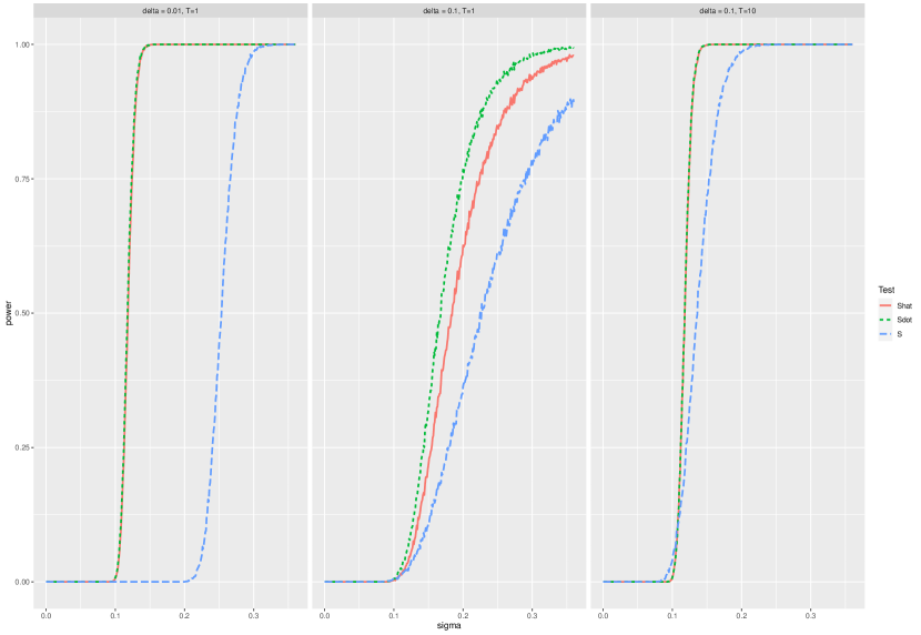
Figure 1: Power functions of the test of $H_{0}:\sigma^{2}=0.1^{2}$ against $H_{1}:\sigma^{2}>0.1^{2}$ as a function of $\sigma_{20}^{2}$. Processes $X_{\sigma}$ are simulated for $\sigma_{20}^{2}$ varying between $0$ and $0.36$. Three tests are considered: the one-dimensional non-centered test $S$ with known drift (Section 2.1) in dashed blue line, with centered statistic $\dot{S}$ (Section 2.2) in dotted green line, with centered statistics and estimated drift $\tilde{S}$ (Section 2.3) in plain red line. Three designs are considered: $\Delta=0.01,T=1$ (left), $\Delta=0.1,T=1$ (middle) and $\Delta=0.1,T=10$ (right).

All three power functions are plotted on Figure 1. The performance of the centered statistics in tests $\dot{\Upsilon}$ and $\tilde{\Upsilon}$ are almost identical and depend mostly on the number of available observations. The performance of the non-centered test $\Upsilon$ is sensitive to the step size $\Delta$.

Especially the power functions $\Pi(\dot{\Upsilon})$ and $\Pi(\tilde{\Upsilon})$ are identical when $T=10,\Delta=0.1$ and $T=1,\Delta=0.01$. This is in accordance with the concluding remark in Section 2.2: the performance of the test does not depend on the time horizon nor on the step size, only on the number of observations. For the non-centered statistics $\Pi(\Upsilon)$, however, it is not the case: as the law of the statistics depends on the drift, the performance of the test depends both on the number of observations, and on the discretization step.

5.2 2-dimensional process with known drift

To illustrate how the method works in dimension two, we use a randomly perturbed sinusoïd $X_{t}=(X_{t,1},X_{t,2})$:

$$\begin{gathered}dX_{t,1}=\theta_{1}\sin(t)dt+\sigma_{1}dW_{t,1},\\ dX_{t,2}=\theta_{2}\cos(t)dt+\sigma_{2}dW_{t,2}.\end{gathered}$$ (33)

Parameters used for simulations are $X_{0,1}=X_{0,2}=0,\theta_{1}=\theta_{2}=1$, $\sigma_{2}=1$. We generate $N=5000$ processes under $H_{1}$ with $\sigma^{2}_{1}$ varying between $0$ and $0.36$ (with a step $0.001$) in order to study the power of the test. We use 3 different scenarios: with $T=1,\Delta=0.01$; $T=1,\Delta=0.1$ and $T=10,\Delta=0.1$.

We define the power function as in (32) for the 2-dimensional tests with known drift (Section 3.2) or estimated (Section 3.3), and for the multiple testing procedure (Section 4) with either known drift, or estimated.

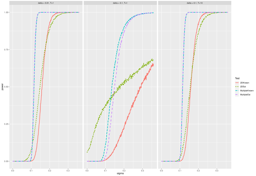
Figure 2: Power functions of the test of $H_{0}:\sigma_{1}^{2}\sigma_{2}^{2}=\sigma_{20}^{2}$ against $H_{1}:\sigma_{1}^{2}\sigma_{2}^{2}>\sigma_{20}^{2}$ as a function of $\sigma_{20}^{2}$. Processes $X_{\sigma}$ are simulated for $\sigma_{20}^{2}$ varying between $0$ and $0.36$. Four tests are considered: the 2-dimensional test with known drift (Section 3.2) in plain red line, with estimated drift (Section 3.3) with dotted green line, the multiple testing procedure (Section 4) with known drift in blue dot-dashed line and estimated drift in magenta dashed line. Three designs are considered: $\Delta=0.01,T=1$ (left), $\Delta=0.1,T=1$ (middle) and $\Delta=0.1,T=10$ (right).

Results are presented in Figure 2. For 2-dimensional tests, the power is influenced by the number of observations $n$. When $\Delta=0.1,T=10$, the powers are almost identical to the case $\Delta=0.01,T=1$. This is in accordance with the remark following Theorem 2, the separation rate of the two hypotheses depends only on the number of observations. Unsurprisingly, in the scenario with very few observations ($\Delta=0.1,T=1$), the hypotheses fail to separate even when $\sigma^{2}>>\sigma^{2}_{0}$. When the parameters of the drift are estimated, the power of the test is slightly smaller. This is expected as the test statistic is build only on half of the sample (the first half sample being used to estimate the parameters).

The multiple testing gives better results. For both known and estimated drift, the multiple test gives a perfect separation already at $\sigma=0.14$ (for settings $\Delta=0.01,T=1$ and $\Delta=0.1,T=10$), while for the two-dimensional test a separation occurs closer to $\sigma=0.25$.

6 Conclusions

We develop various tests of the diffusion coefficients of SDEs. In dimension one, we propose a test statistic that has an explicit distribution, even when the (linear) drift parameter is unknown. The tests are of exact level $\alpha$. We also prove separability conditions to achieve a given power. The test with an unknown parameter can be applied to a non-parametric drift estimated by a projection on a functional basis, e.g. on a spline basis. It can therefore be used to test the diffusion coefficient of a one-dimensional SDE even when the drift is unknown.

In dimension 2, we propose a test statistic, with a non-explicit distribution. However, thanks to concentration inequalities, we prove a test procedure with a non-asymptotic level. When the drift parameter is unknown, the test procedure is adapted by estimating the parameters on the first half of the sample and then applying the test statistic using data from the second half of the sample. We therefore loose power when the parameters are estimated, as the simulations also illustrate.

We therefore propose an alternative, which is also suitable for a dimension $d$ greater than 2. This alternative uses a one-dimensional test on each coordinate and corrects the procedure by a multiple testing approach. This allows to control the type I error of the global test. Since the one-dimensional tests have the exact level even when the linear drift parameters are estimated, the multiple testing procedure detects the diffusion coefficient with the exact level, even when the drift is estimated on a functional basis (spline basis, for example).

Further work would involve considering SDE whose drift depends on the process itself. The main difficulty lies in the fact that the increments are then non-independent. Proving the upper and lower bounds of the test statistics would require further concentration inequalities.

Appendix A Appendix

Proofs for 1-D SDE

Proof of Lemma 2.

We only prove (ii) as (i) is trivial. Note that

$\left(X_{(i+1)\Delta}-X_{i\Delta}\right)\sim\mathcal{N}\left(\theta\int_{(i-1)\Delta}^{i\Delta}f_{s}ds,\Delta\sigma^{2}\right)$ and the increments are independent. As $\hat{\theta}$ is normally distributed as a linear combination of normal variables, it is easy to see that $\mathbb{E}(\hat{\theta})=\theta$ and

$$Var\left[\hat{\theta}\right] = \frac{\sum_{i=1}^{n}Var\left[X_{(i+1)\Delta}-X_{i\Delta}\right]\left({\int_{(i-1)\Delta}^{i\Delta}f_{s}ds}\right)^{2}}{\left(\sum_{i=1}^{n}\left(\int_{(i-1)\Delta}^{i\Delta}f_{s}ds\right)^{2}\right)^{2}}$$

$$= \frac{\Delta\sigma^{2}}{\sum_{i=1}^{n}\left(\int_{(i-1)\Delta}^{i\Delta}f_{s}ds\right)^{2}}.$$

∎

Proof of Lemma 3.

Let us introduce for $i=1,\ldots,n$, $Y_{i}=\frac{X_{i\Delta}-X_{(i-1)\Delta}}{\sqrt{\Delta}}$ and the corresponding vector $Y=(Y_{1},\ldots,Y_{n})^{t}$, such that $Y=Z\theta+\varepsilon$, with $\varepsilon\sim\mathcal{N}(0,\sigma^{2}I)$. Thus $\hat{\theta}=(Z^{t}Z)^{-1}Z^{t}Y$ and $\hat{\xi}_{i}=Y_{i}-Z_{i}\hat{\theta}$. Then we have $\hat{\xi}=(I-H)Y$ and $\hat{\xi}$ follows a normal distribution with variance $\sigma^{2}(I-H)$ (because $I-H$ is a projection matrix). Note that $\sum_{i=1}^{n}H_{ii}=1$ and $rank(H)=1$. Thus $rank(C^{t}C)=n-1$ and we can deduce the last point. ∎

Proof of Proposition 4.

First, note that by Theorem 4.1.1. in Girko (1990) $\dot{s}_{i}\sim\sigma^{2}_{1}\sigma^{2}_{2}\chi^{2}_{i,1}\chi^{2}_{i,2}$, where $\chi^{2}_{i,k}$ denotes a variable distributed according to a chi-squared distribution with $k$ degrees of freedom, all variables being independent in $i$. Here we use the advantage that the covariance matrix of each vector-column is the same. The distribution of $\chi^{2}_{i,1}\chi^{2}_{i,2}$ is deduced from Wells et al. (1962) . The PDF of a product $\chi^{2}_{i,1}\chi^{2}_{i,2}$ is written as follows:

$$f(\omega)=\frac{\omega^{-1/4}K_{1/2}(\omega^{1/2})}{\sqrt{2}\Gamma(1)\Gamma(1/2)},$$ (34)

where $K_{v}(x)$ is the modified Bessel function of the second kind. Further, in our specific case, $K_{1/2}(\omega^{1/2})=\frac{1}{2}\sqrt{2\pi}e^{-\sqrt{\omega}}\omega^{-1/4}$, and simplify (34), obtaining:

$$f(\omega)=\frac{1}{2}\frac{\omega^{-1/4}\sqrt{2\pi}e^{-\sqrt{\omega}}\omega^{-1/4}}{\sqrt{2\pi}}=\frac{1}{2}\omega^{-\frac{1}{2}}e^{-\sqrt{\omega}}.$$

We can deduce the expectation:

$$\mathds{E}\left[\dot{s}_{i}\right]=\frac{1}{2}\int_{0}^{\infty}\sqrt{\frac{x}{\sigma^{2}_{1}\sigma^{2}_{2}}}e^{-\sqrt{\frac{x}{\sigma^{2}_{1}\sigma^{2}_{2}}}}dx=2\sigma^{2}_{1}\sigma^{2}_{2}.$$

For the second moment the computation is similar:

$$\mathds{E}\left[\dot{s}^{2}_{i}\right]=\frac{1}{2}\int_{0}^{\infty}\frac{x^{3/2}}{\sqrt{\sigma^{2}_{1}\sigma^{2}_{2}}}e^{-\sqrt{\frac{x}{\sigma^{2}_{1}\sigma^{2}_{2}}}}dx=24\sigma^{4}_{1}\sigma^{4}_{2}.$$

Finally, note that

$$\mathds{P}\left(\dot{s}_{i}\leq x\right)=\mathds{P}\left(\sigma^{2}_{1}\sigma^{2}_{2}\chi^{2}_{i,1}\chi^{2}_{i,2}\leq x\right)=\mathds{P}\left(\chi^{2}_{i,1}\chi^{2}_{i,2}\leq\frac{x}{\sigma^{2}_{1}\sigma^{2}_{2}}\right)=\frac{1}{2}\int_{0}^{\frac{x}{\sigma^{2}_{1}\sigma^{2}_{2}}}\frac{e^{-\sqrt{\omega}}}{\sqrt{\omega}}d\omega.$$

Computing the integral, we obtain the result. ∎

Proofs for 2-D SDE

Proof of Theorem 1.

Proof of 1. First, note that

$$\mathds{P}\left(\dot{S}-\mathds{E}\left[\dot{S}\right]\leq-t\right)=\mathds{P}\left(\sum_{i=1}^{n/2}\left(\dot{s}_{i}-\mathds{E}\left[\dot{s}_{i}\right]\right)\leq-nt/2\right).$$

For all $\lambda>0$, we have:

$$\mathds{P}\left(\sum_{i=1}^{n/2}\left(\dot{s}_{i}-\mathds{E}\left[\dot{s}_{i}\right]\right)\leq-nt/2\right)=\mathds{P}\left(e^{-\lambda(\sum_{i=1}^{n/2}\dot{s}_{i}-\sum_{i=1}^{n/2}\mathds{E}\left[\dot{s}_{i}\right])}\geq e^{\lambda nt/2}\right).$$

Then, by Markov’s inequality, we have:

$$\mathds{P}\left(e^{-\lambda(\sum_{i=1}^{n/2}\dot{s}_{i}-\sum_{i=1}^{n/2}\mathds{E}\left[\dot{s}_{i}\right])}\geq e^{\lambda nt/2}\right)\leq\mathds{E}\left[e^{-\lambda(\sum_{i=1}^{n/2}\dot{s}_{i}-\sum_{i=1}^{n/2}\mathds{E}\left[\dot{s}_{i}\right])}\right]e^{-\lambda nt/2}.$$

Since all the $\dot{s}_{i}$ are independent in $i$, we note that

$$\mathds{E}\left[e^{-\lambda(\sum_{i=1}^{n/2}\dot{s}_{i}-\sum_{i=1}^{n/2}\mathds{E}\left[\dot{s}_{i}\right])}\right]e^{-\lambda nt/2}=e^{-\lambda nt/2}\prod_{i=1}^{n/2}\mathds{E}\left[e^{-\lambda(\dot{s}_{i}-\mathds{E}\left[\dot{s}_{i}\right])}\right]\\ =e^{-\lambda nt/2+\lambda\sum_{i=1}^{n/2}\mathds{E}\left[\dot{s}_{i}\right]}\prod_{i=1}^{n/2}\mathds{E}\left[e^{-\lambda\dot{s}_{i}}\right].$$

Now, let us rewrite:

$$\mathds{E}\left[e^{-\lambda\dot{s}_{i}}\right]=1-\lambda\mathds{E}[\dot{s}_{i}]+\lambda^{2}\mathds{E}\left[\dot{s}^{2}_{i}\frac{e^{-\lambda\dot{s}_{i}}+\lambda\dot{s}_{i}-1}{\left(\lambda\dot{s}_{i}\right)^{2}}\right].$$

Now, let us define the following function:

$$h(u):=\frac{e^{-u}+u-1}{u^{2}},$$

which is decreasing for any $u>0$ [REF]. For $\lambda>0$ and as $\dot{s}_{i}\geq 0$, we have:

$$h\left(\lambda\dot{s}_{i}\right)\leq h(0)=1.$$

Then, $\mathds{E}\left[\dot{s}^{2}_{i}h\left(\lambda\dot{s}_{i}\right)\right]\leq\mathds{E}\left[\dot{s}^{2}_{i}\right]$ and $\mathds{E}\left[e^{-\lambda\dot{s}_{i}}\right]\leq 1-\lambda\mathds{E}[\dot{s}_{i}]+\lambda^{2}\mathds{E}\left[\dot{s}^{2}_{i}\right]$. Finally, we obtain:

$$\mathds{P}\left(e^{-\lambda(\dot{S}-\mathds{E}\left[\dot{S}\right])}\geq e^{\lambda t}\right)\leq e^{-\lambda nt/2+\lambda\sum_{i=1}^{n/2}\mathds{E}\left[\dot{s}_{i}\right]}\prod_{i=1}^{n/2}\left(1-\lambda\mathds{E}[\dot{s}_{i}]+\lambda^{2}\mathds{E}\left[\dot{s}^{2}_{i}\right]\right)\\ \leq\exp\left(-\lambda nt/2+\lambda\sum_{i=1}^{n/2}\mathds{E}\left[\dot{s}_{i}\right]-\lambda\sum_{i=1}^{n/2}\mathds{E}[\dot{s}_{i}]+\lambda^{2}\sum_{i=1}^{n/2}\mathds{E}\left[\dot{s}^{2}_{i}\right]\right)\\ =\exp\left(-\lambda nt/2+\lambda^{2}\sum_{i=1}^{n/2}\mathds{E}\left[\dot{s}^{2}_{i}\right]\right).$$ (35)

Then we maximize the last expression with respect to $\lambda$. The maximum is obtained for $\hat{\lambda}=\frac{nt}{4\sum_{i=1}^{n/2}\mathds{E}\left[\dot{s}^{2}_{i}\right]}.$ Using $\mathds{E}\left[\dot{s}^{2}_{i}\right]=24\sigma^{4}_{1}\sigma^{4}_{2}$ (Proposition 4), we obtain the bound

$$\exp\left(-\hat{\lambda}nt/2+\hat{\lambda}^{2}\sum_{i=1}^{n/2}\mathds{E}\left[\dot{s}^{2}_{i}\right]\right)=\exp\left(-\frac{(nt/2)^{2}}{4\sum_{i=1}^{n/2}\mathds{E}\left[\dot{s}^{2}_{i}\right]}\right)=\exp\left(-\frac{(nt/2)^{2}}{n48\sigma^{4}_{1}\sigma^{4}_{2}}\right).$$

It gives the result.

Proof of 2. By Chebyshev’s inequality we have

$$\mathds{P}\left(\left|\sum_{i=1}^{n/2}\dot{s}_{i}-\mathds{E}\left[\sum_{i=1}^{n/2}\dot{s}_{i}\right]\right|\geq nt/2\right)\leq\frac{Var\left[\sum_{i=1}^{n/2}\dot{s}_{i}\right]}{\left(nt/2\right)^{2}}.$$

It implies:

$$\mathds{P}\left(\sum_{i=1}^{n/2}\dot{s}_{i}-\mathds{E}\left[\sum_{i=1}^{n/2}\dot{s}_{i}\right]\geq nt/2\right)\\ \\ \leq\frac{Var\left[\sum_{i=1}^{n/2}\dot{s}_{i}\right]}{\left(nt/2\right)^{2}}-\mathds{P}\left(\sum_{i=1}^{n/2}\dot{s}_{i}-\mathds{E}\left[\sum_{i=1}^{n/2}\dot{s}_{i}\right]\leq-nt/2\right).$$

Note that $\mathds{P}\left(\sum_{i=1}^{n/2}\dot{s}_{i}-\mathds{E}\left[\sum_{i=1}^{n/2}\dot{s}_{i}\right]\leq-nt/2\right)$ is evaluated in 23 and is decaying exponentially fast as $t$ grows. In comparison, the first term is decaying at much slower rate. Thus, the principal term which controls the upper bound is given by $\frac{Var\left[\sum_{i=1}^{n/2}\dot{s}_{i}\right]}{\left(nt/2\right)^{2}}$. Finally, the following result is obtained:

$$\mathds{P}\left(\dot{S}-\mathds{E}\left[\dot{S}\right]\geq t\right)\leq\frac{10n\sigma^{4}_{1}\sigma^{4}_{2}}{\left(nt/2\right)^{2}}=\frac{40}{nt^{2}}\sigma^{4}_{1}\sigma^{4}_{2}.$$

∎

Sharp estimate on classical quantiles

Lemma 7.

For any $\alpha\in(0,0.5]$, we always have that

$$q_{\mathcal{N},1-\alpha}\leq\sqrt{2\log(1/\alpha)}$$

and that

$$q_{\chi_{n}^{2}(\lambda),1-\alpha}\leq(\sqrt{n}+\sqrt{2\log(1/\alpha)})^{2}+2\sqrt{2\log(1/\alpha)}\lambda^{1/2}+\lambda.$$

With $\alpha=0.5$, we get the slightly better bound

$$q_{\chi_{n}^{2}(\lambda),0.5}\leq(\sqrt{n}+\sqrt{2\log(2)})^{2}+\lambda.$$

Moreover if $\alpha\leq 1/\sqrt{2\pi}\simeq 0.39,$ we also have that

$$q_{\mathcal{N},1-\alpha}\geq\sqrt{\log(1/\alpha)}$$

and

$$q_{\chi_{n}^{2}(\lambda),1-\alpha}\geq n-1+2\sqrt{\log(1/\alpha)}\lambda^{1/2}+\lambda+\log(1/\alpha).$$

For $\beta<0.5$, we have the following bound

$$q_{\chi_{n}^{2}(\lambda),\beta}\geq n+\lambda-\sqrt{\frac{2(n+2\lambda)}{\beta}}.$$

Proof.

Gordon (1941) establishes that if $\Phi(x)$ is the c.d.f. of $\mathcal{N}(0,1)$ then for all positive $x$,

$$\frac{e^{-x^{2}/2}}{\sqrt{2\pi}\left(x+x^{-1}\right)}\leq\Phi(x)\leq\frac{e^{-x^{2}/2}}{\sqrt{2\pi}x}.$$

Since the function $f(x)=\frac{e^{-x^{2}/2}}{x}$ is strictly decreasing, we can obtain an upper bound on the quantile by finding a $z_{\alpha}$ such that $f(z_{\alpha})\leq\sqrt{2\pi}\alpha$ for $\alpha<0.5$. Choosing $x_{\alpha}=\sqrt{2\log(1/\alpha)}$, we get $f(x_{\alpha})=\frac{\alpha}{\sqrt{2\log(1/\alpha)}}\leq\sqrt{2\pi}\alpha$ since $\alpha<0.5$.

For the lower bound of the Gaussian quantile, note that for all $v>0$, $v-\log(v)\geq 1$, so $x_{t}=\sqrt{2\log(1/t)-2\log\log(1/t)}$ is well defined for all $t\leq 1$ and satisfies $x_{t}\geq\sqrt{2}$, for all $t\leq 1$. So Gordon’s lower bound implies that

$$\Phi(x_{t})\geq\frac{1}{2\sqrt{2\pi}}f(x_{t})=\frac{t\log(1/t)}{2\sqrt{2\pi}\sqrt{2\log(1/t)-2\log\log(1/t)}}.$$

But $v^{2}/4\geq 2v-2\log(v)$ holds for all positive $v$, so

$$\log(1/t)^{2}/4\geq 2\log(1/t)-2\log\log(1/t)$$

and $\Phi(x_{t})\geq\frac{t}{\sqrt{2\pi}}.$

By taking $t=\sqrt{2\pi}\alpha$, we get therefore that lower bound

$$q_{\mathcal{N},1-\alpha}\geq\sqrt{2\log(\sqrt{2\pi}/\alpha)-2\log\log(\sqrt{2\pi}/\alpha)}.$$

It holds for all $\alpha\leq 1/\sqrt{2\pi}$.

But by studying the function we can see that

$$2\log(\sqrt{2\pi}/\alpha)-2\log\log(\sqrt{2\pi}/\alpha)\geq\log(1/\alpha).$$

For the chi-square distribution with central parameter $\lambda$, we use the results by Robert (1990), which states that

$$q_{\chi_{n}^{2}(\lambda),1-\alpha}\leq q_{\chi_{n}^{2}(0),1-\alpha}+2q_{\mathcal{N},1-\alpha}\lambda^{1/2}+\lambda.$$

We use Gaussian concentration of measure (Boucheron et al., 2013) to derive that, if $X$ is a standard Gaussian vector of dimension $n$ and $\|X\|$ designs its euclidean norm, then for all positive $x$

$$\mathbb{P}(\|X\|\geq\mathbb{E}(\|X\|)+x)\leq e^{-x^{2}/2}.$$

Since $\mathbb{E}(\|X\|)\leq\sqrt{n}$, we have that

$$\mathbb{P}\left(\|X\|^{2}\geq(\sqrt{n}+\sqrt{2\log(1/\alpha)})^{2}\right)\leq\alpha.$$

Combined with the bound on the Gaussian quantiles, it give us the upper bound. For $\alpha=0.5,$ note that $q_{\mathcal{N},1-\alpha}=0$.

For the lower bound, Robert (1990) also proves that

$$q_{\chi_{n}^{2}(\lambda),1-\alpha}\geq n-1+q_{\mathcal{N},1-\alpha}^{2}+2q_{\mathcal{N},1-\alpha}\lambda^{1}/2+\lambda.$$

Combined with the lower bound on Gaussian quantiles, we get the corresponding lower bound.

For the rougher bound for small $\beta$, note that if $Z\sim\chi^{2}_{n}(\lambda)$ then

$$\mathbb{E}(Z)=n+\lambda\quad\mbox{and}\quad Var(Z)=2(n+2\lambda).$$

So by Bienaymé Tchebicheff inequality, we obtain for all positive $x$

$$\mathbb{P}(Z\leq\mathbb{E}(Z)-x)\leq\frac{Var(Z)}{x^{2}}.$$

So by choosing $x=\sqrt{\frac{2(n+2\lambda)}{\beta}}$, we obtain the desired lower bound. ∎

References

• Ableidinger et al. (2017) M. Ableidinger, E. Buckwar, and H. Hinterleitner. A stochastic version of the jansen and rit neural mass model: Analysis and numerics. The Journal of Mathematical Neuroscience, 7(1):1, August 2017.
• Boucheron et al. (2013) Stéphane Boucheron, Gábor Lugosi, and Pascal Massart. Concentration inequalities: A nonasymptotic theory of independence. Oxford university press, 2013.
• Dette and Podolskij (2008) H. Dette and M. Podolskij. Testing the parametric form of the volatility in continuous time diffusion models- an empirical process approach. Journal of Econometrics, 1438:56–73, 2008.
• Ditlevsen and Löcherbach (2017) S. Ditlevsen and E. Löcherbach. Multi-class oscillating systems of interacting neurons. Stoch. Proc. Appl., 127:1840–1869, 2017.
• Ditlevsen and Samson (2014) S. Ditlevsen and A. Samson. Estimation in the partially observed stochastic morris-lecar neuronal model with particle filter and stochastic approximation methods. Ann Applied Stat, 2:674–702, 2014.
• Fissler and Podolskij (2017) T. Fissler and M. Podolskij. Testing the maximal rank of the volatility process for continuous diffusions observed with noise. Bernoulli, 23:3012–3066, 2017.
• Gil et al. (2014) A. Gil, J. Segura, and N. M Temme. The asymptotic and numerical inversion of the marcum q-function. Studies in Applied Mathematics, 133(2):257–278, 2014.
• Girko (1990) V. Girko. Theory of Random Determinants. Springer, 1990. doi: 10.1007/978-94-009-1858-0.
• Goldwyn and Shea-Brown (2011) Joshua H. Goldwyn and Eric Shea-Brown. The what and where of adding channel noise to the hodgkin-huxley equations. 2011. doi: 10.1371/journal.pcbi.1002247.
• Gordon (1941) R.D. Gordon. Values of mills’ ratio of area to bounding ordinate and of the normal probability integral for large values of the argument. The Annals of Mathematical Statistics, 12(3):364–366, 1941.
• Höpfner et al. (2016) R Höpfner, E Löcherbach, M Thieullen, et al. Ergodicity for a stochastic hodgkin–huxley model driven by ornstein–uhlenbeck type input. In Annales de l’Institut Henri Poincaré, Probabilités et Statistiques, volume 52, pages 483–501, 2016.
• Jacod and Podolskij (2013) J. Jacod and M. Podolskij. A test for the rank of the volatility process: the random perturbation approach. The Annals of Statistics, 41(5):2391–2427, 2013.
• Jacod et al. (2008) J. Jacod, A. Lejay, and D. Talay. Estimation of the brownian dimension of a continuous itô process. Bernoulli, 14(2):469–498, 2008.
• León and Samson (2018) J.R. León and A. Samson. Hypoelliptic stochastic FitzHugh-Nagumo neuronal model: mixing, up-crossing and estimation of the spike rate. Annals of Applied Probability, 28:2243–2274, 2018.
• Podolskij and Rosenbaum (2012) M. Podolskij and M. Rosenbaum. Testing the local volatility assumption: a statistical approach. Annals of Finance, 8:31–48, 2012.
• Reiss and Winkelmann (2021) M. Reiss and L. Winkelmann. Inference on the maximal rank of time-varying covariance matrices using high-frequency data. submitted, 23:3012–3066, 2021.
• Robert (1990) C. Robert. On some accurate bounds for the quantiles of a non-central chi squared distribution. Statistics and Probability Letters, 10(2):101–106, 1990.
• Roquain (2011) Etienne Roquain. Type i error rate control for testing many hypotheses: a survey with proofs. Journal de la Société Française de Statistique, 152(2):3–38, 2011.
• Valettas (2019) P. Valettas. On the tightness of gaussian concentration for convex functions. Journal d’Analyse Mathématique, 139:341–367, 2019.
• Wells et al. (1962) WT Wells, RL Anderson, John W Cell, et al. The distribution of the product of two central or non-central chi-square variates. The Annals of Mathematical Statistics, 33(3):1016–1020, 1962.