Magnon Spin Photogalvanic Effect in Collinear Ferromagnets

Abstract

We propose a spin photogalvanic effect of magnons with broken inversion symmetry. The dc spin photocurrent is generated via the Aharonov-Casher effect, which includes the Drude, Berry curvature dipole, shift, injection, and rectification components with distinct quantum geometric origin. Based on a symmetry classification, we uncover that there exist linearly polarized (LP) magnon spin photocurrent responses in the breathing kagome-lattice ferromagnet with Dzyaloshinskii-Moriya interaction, and the circularly polarized (CP) responses due to the symmetry breaking by applying a uniaxial strain. We address that the topological phase transitions can be characterized by the spin photocurrents. This study presents a deeper insight into the nonlinear responses of light-magnon interactions, and suggests a possible way to generate and control the magnon spin current in real materials.

Spin transport plays a central role in the field of spintronics [1, 2]. Currently there are significant interests to explore the magnons in magnetic materials. The magnons, as collective spin excitations of magnetically ordered materials, are electrically neutral bosonic quasiparticles. The transport of magnons obviates Joule heating at a fundamental level, and thus magnons are regarded as the candidate in pursuing the next-generation spintronics [3, 4]. For this purpose, a deeper understanding of the properties of magnons and the precise manipulation of magnons are urgently called for. Much progress has been made in studying the thermal control on magnons [5, 6, 7, 8, 9, 10, 11, 12, 13, 14, 15, 16, 17, 18, 19].

However, due to the electrical neutrality of the magnons, their coupling to the external electric field is less considered. The magnons are expected to be generated and transferred by optical excitations. It has been proposed that the dc magnon spin photocurrent can be generated by the Zeeman coupling of the magnetic field component of the light [20, 21, 22]. Since the component of magnetic field of light is much weaker than that of electric field, large spin current responses through the above mechanisms require high intensity of light. Therefore, a desired goal is to achieve an enhanced magnon spin photocurrent by the electric field component of the light. For example, the spin current driven by circularly polarized light was proposed via a two magnon Raman process with the coupling to the electric field [23]. The magnetoelectric coupling generally exists in multiferroic materials, for which the magnon can be generated and controlled by electric field [24, 25, 26]. Recently, the dc magnon spin photocurrents has been predicted in collinear antiferromagnets via the coupling between electric field and polarization with a broken inversion symmetry [27]. However, the spin photocurrent induced by the interaction between the electric field and the magnons has not been fully understood, and it is unclear that how it is affected by the quantum geometry of magnon bands [28].

In this work, we develop a general theory for the magnon spin photogalvanic effect (SPGE) in ordered ferromagnetic insulators. In analogy to the dc charge photocurrent responses to the electric field [29, 30, 31, 32, 33, 34, 35, 36], the magnon SPGE is a dc spin photocurrent response

$$J_{s}=\chi^{\alpha\alpha_{1}\alpha_{2}}E^{\alpha_{1}}(\Omega)E^{\alpha_{2}}(-\Omega),$$ (1)

with $\Omega$ being the frequency of the light. The magnon moving in an electric field acquires a geometric phase through the Aharonov-Casher (AC) effect. The AC phase accumulated by magnon hopping is given by [37, 38, 39, 40]

$$\theta_{ij}=\frac{g\mu_{B}}{\hbar c^{2}}\int_{\bm{r}_{i}}^{\bm{r}_{j}}(\bm{E}(t)\times\hat{\bm{z}})\cdot d\bm{r},$$ (2)

where the magnetization is assumed along $z$-direction. The interaction with electric field is incorporated into the magnon Hamiltonian via an effective gauge potential caused by AC phase. Consequently, the nonlinear spin photocurrent can be handled with standard perturbation theory. We show that $\chi^{\alpha\alpha_{1}\alpha_{2}}\propto\epsilon^{\alpha_{1}z\beta}\epsilon^{\alpha_{2}z\gamma}$ ($\epsilon^{\alpha_{2}z\gamma}$ is the Levi-Civita symbol). That is, the electric field is restricted into the plane perpendicular to the axis of magnetization, attributed to the orthogonality between the electric field and the magnon magnetic moment, as illustrated in Eq. (2). While for the charge photocurrent there is no such constraint, making it be a prominent character.

Let us start with a general two-body spin interaction Hamiltonian in the absence of external field,

$$H_{0}=\frac{1}{2}\sum_{i,j}^{L}\sum_{n,m}^{N}\sum_{\alpha\beta}{S}^{\alpha}_{i,n}H^{\alpha\beta}_{nm}(i-j){S}^{\beta}_{j,m},$$ (3)

where $\bm{S}_{i,n}$ is a spin operator at the $n$th sublattice (with total number $N$) of the $i$th magnetic unit cell (with total number $L$), with $H^{\alpha\beta}_{nm}(i-j)$ the magnetic exchange interaction. For a collinear ferromagnet, if the magnetization is along the $z$-direction, the spin-wave approximation is expressed by the Holstein–Primakoff transformation [41]

$$\bm{S}_{i,n}^{\alpha}=\sqrt{\frac{S}{2}}\hat{\bm{u}}_{n}a_{i,n}+\sqrt{\frac{S}{2}}\hat{\bm{u}}_{n}^{*}a_{i,n}^{\dagger}+\hat{\bm{z}}_{n}(S-a_{i,n}^{\dagger}a_{i,n}),$$ (4)

with $\bm{u}_{n}\equiv\hat{\bm{x}}_{n}+i\hat{\bm{y}}_{n}$, and $\{\hat{\bm{x}}_{n},\hat{\bm{y}}_{n},\hat{\bm{z}}_{n}\}$ is the set of basis vectors of the rotating frame where $\hat{\bm{z}}_{n}$ is the direction of classical spin at $n$. The corresponding quadratic form of boson Hamiltonian is given by $H=\sum_{\bm{k}}\Psi_{\bm{k}}^{\dagger}\mathcal{H}_{\bm{k}}\Psi_{\bm{k}}$, where $\Psi_{\bm{k}}^{\dagger}=(a_{{\bm{k}},1}^{\dagger},\cdots,a_{{\bm{k}},N}^{\dagger})$. A direct diagonalization by the unitary matrix $U_{\bm{k}}$ gives $H=\sum_{\bm{k}}\mathcal{E}_{\bm{k}}\Phi_{\bm{k}}^{\dagger}\Phi_{\bm{k}}$, where $U^{\dagger}_{\bm{k}}\mathcal{H}_{\bm{k}}U_{\bm{k}}=\mathcal{E}_{\bm{k}}$ and $\Psi_{\bm{k}}=U_{\bm{k}}\Phi_{\bm{k}}$.

Quantum kinetic equations in the presence of the AC phase.– Making use of the Peierls substitution, the electric field modifies the kinetic part of the noninteracting Hamiltonian, which is accounted for by replacing the canonical momentum $\bm{k}$ via the minimal coupling $\mathcal{H}(\bm{k})=\mathcal{H}_{0}(\bm{k}+\frac{g\mu_{B}}{c}\bm{A}^{E})$ by introducing an “electric” vector potential potential $\bm{A}^{E}\equiv\frac{1}{c}\bm{E}\times\hat{\bm{e}}_{z}$ [42, 43, 44, 45] (see Sec. II in SM [41] for more details). Alternatively, by use of gauge transformation, an effective “electric field” is taken into account in form of the dipole interaction (see Sec. III in SM [41])

$$\mathcal{H}(t)=\mathcal{H}_{0}\left(\bm{k}\right)+\frac{g\mu_{B}}{c}\tilde{\bm{E}}(t)\cdot\bm{r},$$ (5)

in which the effective “electric field” is given by $\tilde{\bm{E}}(t)=-\partial\bm{A}^{E}/\partial t$.

We derive the nonlinear optical conductivity by following the density matrix approach. The reduced density matrix (RDM) in band space is given by the average of the product of a creation and a destruction operator in Bloch states $\rho_{\bm{k}mn}(t)\equiv\langle\Phi_{\bm{k}m}^{\dagger}\Phi_{\bm{k}n}\rangle$. The time evolution of the RDM is obtained via von Neumann equation (see Sec. V in SM [41])

$$\left(\partial_{t}+i\varepsilon_{\bm{k}mn}/\hbar\right)\rho_{\bm{k}mn}(t)=\mathcal{D}_{\text{opt}}[\rho(t)]_{\bm{k}mn}.$$ (6)

Here, we define $\varepsilon_{\bm{k}mn}=\varepsilon_{\bm{k}m}-\varepsilon_{\bm{k}n}$. $\mathcal{D}_{\text{opt}}$ is the optical driving term, and it acts on operator via

$$\mathcal{D}_{\text{opt}}[O]=\frac{g\mu_{B}}{\hbar c^{2}}\bm{E}\times\bm{e}_{z}\cdot\bm{D}[O].$$ (7)

The covariant derivative operator acts on operators via [46, 32]

$$(\bm{D}_{\bm{k}}\mathcal{O}_{\bm{k}})_{mn}=\nabla_{\bm{k}}\mathcal{O}(\bm{k})_{mn}-i[\bm{\mathcal{A}}_{\bm{k}},{\mathcal{O}}(\bm{k})]_{mn},$$ (8)

where $\bm{\mathcal{A}}_{\bm{k}}$ is the Berry connection whose matrix elements are $\bm{\mathcal{A}}_{\bm{k}mn}=i\langle u_{\bm{k}m}\left|\bm{\nabla}_{\bm{k}}u_{\bm{k}n}\right>$, with $\left|u_{\bm{k}n}\right>$ the periodic part of the Bloch functions. For convenience, we will not write the $\bm{k}$ index explicitly in the following unless otherwise specified. The density matrix is expanded into contributions of different powers on the external field as $\rho=\sum_{n=0}\rho^{(n)}$, where the zero-order one is the Bose-Einstein distribution $\rho^{(0)}_{\bm{k}mn}=g_{\bm{k}m}\delta_{mn}$. The recursion equations for the RDMs are obtained as

$$\rho^{(n+1)}_{mn}(\omega)= d_{mn}(\omega)\int\frac{d\omega_{1}}{2\pi}\omega_{1}\mathcal{D}_{\text{opt}}[{\rho}^{(n)}(\omega-\omega_{1})]_{mn},$$ (9)

with $d_{mn}(\omega)=1/(\hbar\omega+i0^{+}-\varepsilon_{mn})$.

Table 1: Different terms leading to the magnon SPGE (see Eq. (11)). The spin photoconductivities are evaluated in terms of the following gauge invariant quantities: group velocity $v_{m}^{\alpha}=\frac{1}{\hbar}\partial^{\alpha}\varepsilon_{m}$, where $\partial^{\alpha}=\partial/\partial k_{\alpha}$; velocity difference $\Delta_{mn}^{\alpha}=v_{m}^{\alpha}-v_{n}^{\alpha}$; Berry curvature $\Omega_{m}^{\tau}=\epsilon^{\alpha\gamma\tau}\partial^{\gamma}\mathcal{A}_{nn}^{\tau}$; band-resolved quantum metric (Berry curvature) $G_{mn}^{\beta\gamma}=\{\mathcal{A}_{mn}^{\beta},\mathcal{A}_{nm}^{\gamma}/2\}$ ($\Omega_{mn}^{\beta\gamma}=i[\mathcal{A}_{mn}^{\beta},\mathcal{A}_{nm}^{\gamma}]$); shift vector $R_{mn}^{\alpha\alpha_{1}}=\mathcal{A}_{mm}^{\alpha}-\mathcal{A}_{nn}^{\alpha}-\partial^{\alpha}\arg\mathcal{A}_{mn}^{\alpha_{1}}$; chiral shift vector $R_{mn}^{\alpha,\pm}=\mathcal{A}_{mm}^{\alpha}-\mathcal{A}_{nn}^{\alpha}-\partial^{\alpha}\arg\mathcal{A}_{mn}^{\pm}$ with the Berry connection in circular representation $\mathcal{A}_{mn}^{\pm}=\frac{1}{\sqrt{2}}(\mathcal{A}_{mn}^{x}\pm i\mathcal{A}_{mn}^{y})$. The conductivities can be written as $\eta^{\alpha\alpha_{1}\alpha_{2}}=(\nu_{c}/2)\int[d\bm{k}]\mathcal{I}^{\alpha\alpha_{1}\alpha_{2}}$ and $\kappa^{\alpha\alpha_{1}\alpha_{2}}=(\nu_{c}/2)\int[d\bm{k}]\mathcal{K}^{\alpha\alpha_{1}\alpha_{2}}$ with $\mathcal{I}$ and $\mathcal{K}$ being the integrand, $\nu_{c}$ being the constant $g^{2}\mu_{B}^{2}/(\hbar^{2}c^{4})$. The symbols $\updownarrow$ and $\circlearrowleft$ denote photocurrents induced by LP and CP light, respectively. Note that the LP responses include a factor $\varsigma=1$ for $\alpha_{1}=\alpha_{2}$ and $\varsigma=-1$ for $\alpha_{1}\neq\alpha_{2}$. A phenomenological scattering rate $\Gamma$ is introduced for the injection current.

Current	Spin photoconductivity	$\mathcal{T}^{\prime}$	$\mathcal{P}\mathcal{T}^{\prime}$	Physical origin
$\text{Durde}\updownarrow$	$\mathcal{I}_{\text{D}}^{\alpha\alpha_{1}\alpha_{2}}=\varsigma(2/\hbar)\sum_{m}v_{m}^{\alpha}\partial^{\alpha_{1}}\partial^{\alpha_{2}}g_{m}$	$\times$	$\checkmark$	Nonequilibrium distribution
$\text{BCD}\circlearrowleft$	$\mathcal{K}_{\text{BCD}}^{\alpha\alpha_{1}\alpha_{2}}=(\Omega/\hbar)\sum_{m}(\epsilon^{\alpha\alpha_{2}\tau}\partial^{\alpha_{1}}-\epsilon^{\alpha\alpha_{1}\tau}\partial^{\alpha_{2}})\Omega_{m}^{\tau}g_{m}$	$\checkmark$	$\times$	Anomalous velocity + nonequilibrium distribution
$\text{Injection}\updownarrow$	$\mathcal{I}_{\text{Inj}}^{\alpha\alpha_{1}\alpha_{2}}=-\varsigma{4\hbar}\sum_{m,n}\frac{\Omega^{2}}{(\hbar\Omega-\varepsilon_{mn})^{2}+\Gamma^{2}}\Delta_{mn}^{\alpha}G_{mn}^{\alpha_{1}\alpha_{2}}g_{mn}$	$\times$	$\checkmark$	Velocity difference + dipole transition
$\text{Injection}\circlearrowleft$	$\mathcal{K}_{\text{Inj}}^{\alpha\alpha_{1}\alpha_{2}}=-{2\pi\hbar}\sum_{m,n}\frac{\Omega^{2}}{(\hbar\Omega-\varepsilon_{mn})^{2}+\Gamma^{2}}\Delta_{mn}^{\alpha}\Omega_{mn}^{\alpha_{1}\alpha_{2}}g_{mn}$	$\checkmark$	$\times$	Velocity difference + dipole transition
$\text{Shift}\updownarrow$	$\mathcal{I}_{\text{Sh}}^{\alpha\alpha_{1}\alpha_{2}}=\varsigma 2\pi\sum_{m,n}\Omega^{2}\delta_{\hbar\Omega-\varepsilon_{mn}}R_{mn}^{\alpha\alpha_{1}}G_{mn}^{\alpha_{1}\alpha_{1}}$	$\checkmark$	$\times$	Position shift + dipole transition
$\text{Shift}\circlearrowleft$	$\quad\mathcal{K}_{\text{Sh}}^{\alpha\alpha_{1}\alpha_{2}}=-4\pi\sum_{m,n}\Omega^{2}\delta_{\hbar\Omega-\varepsilon_{mn}}(R_{mn}^{\alpha,+}\lvert\mathcal{A}_{nm}^{+}\rvert^{2}-R_{mn}^{\alpha,-}\lvert\mathcal{A}_{nm}^{-}\rvert^{2})g_{mn}$	$\times$	$\checkmark$	Position shift + dipole transition
$\text{Rectification}\updownarrow$	$\mathcal{I}_{\text{Rec}}^{\alpha\alpha_{1}\alpha_{2}}=\varsigma 4\sum_{m,n}\frac{\Omega^{2}}{\hbar\Omega-\varepsilon_{mn}}G_{mn}^{\alpha_{1}\alpha_{2}}\partial^{\alpha}g_{mn}$	$\times$	$\checkmark$	Dipole transition +nonequilibrium distribution
$\text{Rectification}\circlearrowleft$	$\mathcal{K}_{\text{Rec}}^{\alpha\alpha_{1}\alpha_{2}}=-\sum_{m,n}\frac{\Omega^{2}}{\hbar\Omega-\varepsilon_{mn}}\Omega_{mn}^{\alpha_{1}\alpha_{2}}\partial^{\alpha}g_{mn}$	$\checkmark$	$\times$	Dipole transition +nonequilibrium distribution

We now define the magnon spin current. Due to the conservation of the $z$ component of the total spin, the local magnon spin density $n(\bm{r}_{i})=\hbar\sum_{m}\bm{z}_{m}a_{i,m}^{\dagger}a_{i,m}$ satisfies the continuity equation $\partial n_{\bm{q}}/\partial t+i\bm{q}\cdot\bm{J}_{s}=0$ ($n_{\bm{q}}$ is Fourier component of the magnon spin density) in the long-wavelength limit. And the magnon spin current operator is found as (see Sec. IV SM [41] for the derivation)

$$\hat{\bm{J}}_{s}=\hbar\sum_{\bm{k}}\Phi_{\bm{k}}^{\dagger}\left(\partial_{\bm{k}}\mathcal{H}_{\bm{k}}-i[\bm{\mathcal{A}}_{\bm{k}},{\mathcal{H}_{\bm{k}}}]\right)\Phi_{\bm{k}}.$$ (10)

The $n$th-order magnon spin current is calculated via $J^{\alpha,(n)}_{s}=\int[d\bm{k}]\text{Tr}[\rho^{(n)}\hat{J}_{s}^{\alpha}]$. The photocurrent response is classified as the linearly polarized and circularly polarized light-induced currents, where the LP (CP)-photocurrent is given by the real symmetric (imaginary antisymmetric) component of the photoconductivity tensor $\eta^{\alpha\alpha_{1}\alpha_{2}}=\frac{1}{2}\text{Re}(\chi^{\alpha\alpha_{1}\alpha_{2}}+\chi^{\alpha\alpha_{2}\alpha_{1}})$, $[\kappa^{\alpha\alpha_{1}\alpha_{2}}=\frac{1}{2}\text{Im}(\chi^{\alpha\alpha_{1}\alpha_{2}}-\chi^{\alpha\alpha_{2}\alpha_{1}})]$. leaving the details of derivation to the SM, we obtain

$$\chi^{\alpha\alpha_{1}\alpha_{2}}=\chi^{\alpha\alpha_{1}\alpha_{2}}_{\text{D}}+\chi^{\alpha\alpha_{1}\alpha_{2}}_{\text{BCD}}+\chi^{\alpha\alpha_{1}\alpha_{2}}_{\text{Inj}}+\chi^{\alpha\alpha_{1}\alpha_{2}}_{\text{Sh}}+\chi^{\alpha\alpha_{1}\alpha_{2}}_{\text{Rec}},$$ (11)

with the functional forms of all the contributions tabulated in Table 1. We denote different contributions as follows: Drude ($\chi^{\alpha\alpha_{1}\alpha_{2}}_{\text{D}}$), Berry curvature dipole (BCD) ($\chi^{\alpha\alpha_{1}\alpha_{2}}_{\text{BCD}}$), injection ($\chi^{\alpha\alpha_{1}\alpha_{2}}_{\text{Inj}}$), shift ($\chi^{\alpha\alpha_{1}\alpha_{2}}_{\text{Sh}}$), and the rectification current ($\chi^{\alpha\alpha_{1}\alpha_{2}}_{\text{Rec}}$). These five terms for magnon spin currents above are all firstly proposed.

The Drude-spin-current (DSC) characters the intra-band effect and classified as a LP spin photocurrent response. Classified as a CP response, the BCD-spin-current (BSC) is originated from a dipole moment of the magnon Berry curvature in momentum space, which scales with the frequency of light and hence vanishes as $\Omega$ approaches to zero. The shift-spin-current (SSC) is justified as the displacement of the magnon wave packet during the interband transition, which is characterized by the shift vector $R_{mn}$. The injection-spin-current (ISC) corresponds to the velocity difference $\Delta_{mn}$ during the interband transition. The SSC and ISC proposed are found as both CP and LP responses. Finally, the rectification spin currents (RSC) as both LP and CP responses are discovered in this work, which are proportional to the derivatives of the distributions, and can be regarded as an analog of the “intrinsic Fermi surface effect” in electronic system [34]. Interestingly, from an inspection of the terms shown in Table 1, it is found that the LP responses (apart from the DSC since it is not geometrical related) are determined by the quantum metric while the CP responses are determined by the Berry curvature. As mentioned, the magnon SSC and ISC were predicted in multiferroic materials [27] with magnon-light coupling through electric polarization, where the shift (injection) spin current is justified as a LP (CP) response. The magnon SPGE induced by AC phase can appear in broader potential materials, including ferromagnets, antiferromagnets and so on.

Symmetry characters.– Let us understand the emergence of magnon SPGE from the symmetry perspective. For a magnet with collinear magnetic order, it is invariant under the combined symmetry operation of the time-reversal $\mathcal{T}$ and a $\pi$ spin rotation about the axis perpendicular to the plane of the magnetic order. This is called the effective time-reversal symmetry $\mathcal{T}^{\prime}$. If systems reserve the effective TRS, there is $\mathcal{T}^{\prime}\mathcal{H}_{\bm{k}}(\mathcal{T}^{\prime})^{-1}=\mathcal{H}_{-\bm{k}}=\mathcal{H}_{\bm{k}}^{*}$ [47, 48]. $\mathcal{T}^{\prime}$ gives a constraint on the Berry connection $\mathcal{A}_{\bm{k}mn}^{\alpha}=\mathcal{A}_{-\bm{k}nm}^{\alpha}$. It implies that $\Omega_{\bm{k}m}^{\tau}=-\Omega_{-\bm{k}m}^{\tau}$ for the Berry curvature. The constraint on other geometric quantities can be obtained similarly (see SM). Now we consider the point-group symmetry transformations. With a point-group symmetry $\mathcal{M}$, the eigenvalues satisfy $\varepsilon_{n\bm{k}}=\varepsilon_{n\mathcal{M}^{-1}\bm{k}}$, and the Berry connection transforms as $\mathcal{A}_{\bm{k}mn}^{\alpha}=\mathcal{M}_{\alpha\beta}\mathcal{A}_{\mathcal{M}^{-1}\bm{k}mn}^{\beta}$. For a general conductivity tensor, one can find that

$$\chi^{\alpha^{\prime}\alpha_{1}^{\prime}\alpha_{2}^{\prime}}=\mathcal{M}^{\alpha^{\prime}\alpha}\mathcal{M}^{\alpha_{1}^{\prime}\alpha_{1}}\mathcal{M}^{\alpha_{2}^{\prime}\alpha_{2}}\chi^{\alpha\alpha_{1}\alpha_{2}}.$$ (12)

Particularly, for a CP response tensor, it is antisymmetric with exchanging the last two indices, and it is convenient to transform it to an equivalent rank-2 pseudotensor $\varpi^{\alpha\beta}=\epsilon^{\beta\alpha_{1}\alpha_{2}}\kappa^{\alpha\alpha_{1}\alpha_{2}}/2$, yielding

$$\varpi^{\alpha^{\prime}\beta^{\prime}}=\det{(\mathcal{M})}\mathcal{M}^{\alpha^{\prime}\alpha}\mathcal{M}^{\beta^{\prime}\beta}\varpi^{\alpha\beta}.$$ (13)

Therefore we obtain the constraints of $\mathcal{T}^{\prime}$ and inversion symmetry $\mathcal{P}$ on the current components, shown in Table 1 (the constraints from all point-group symmetries and their combinations with $\mathcal{T}^{\prime}$ are given in Table SI in SM).

Application to breathing kagome ferromagnet.– Now we present a microscopic calculation of the magnon spin photogalvanic effect. We apply our theory to a breathing kagome-lattice ferromagnets in the absence of inversion symmetry, as shown in Fig. 1 (a). With a nonuniform strain field, the three sublattices are deformed far away (positive perturbation $\delta>0$) or getting closer (negative perturbation $\delta<0$) from their shared corner, as shown in Fig. 1 (b) and (c). The Hamiltonian is written as

$$H=-\sum_{\langle i,j\rangle}J_{ij}\bm{S}_{i}\cdot\bm{S}_{j}+\sum_{\langle i,j\rangle}\bm{D}_{ij}\cdot\bm{S}_{i}\times\bm{S}_{j}.$$ (14)

Here $J>0$ is the nearest-neighbors (NN) ferromagnetic coupling strength. The second term is out-plane NN DMI, where the DM vector is specified as $\bm{D}_{ij}=v_{ij}D\bm{z}$ with $v_{ij}=\pm$, depending on chirality of the triangles in the kagome lattice. In the presence of strain, the values of the exchange interactions are modulated by the small displacements of the spins. Expanding to the linear order around the equilibrium value, the ferromagnetic exchange interaction and the DMI are given by [49, 50] $J_{\pm}=(1\mp\sqrt{3}\eta\delta)J$, $D_{\pm}=(1\mp\sqrt{3}\eta\delta)D$, where subscript $+$ ($-$) denotes intracell (intercell) NN couplings, and $\eta$ is a parameter that describes the response of the couplings to the displacements of sublattices, $\delta$ is the lattice deformation. The bosonic Hamiltonian is written as $\mathcal{H}_{\bm{k}}=\mathcal{H}_{0}-\mathcal{H}_{J}^{NN}-\mathcal{H}_{DM}$, where $\mathcal{H}_{0}=4JI_{3\times 3}$. The nearest neighbour magnetic exchange coupling reads

$$\mathcal{H}_{J}^{NN}=\begin{pmatrix}0&\gamma_{2}&\gamma_{3}^{*}\\ \gamma_{2}^{*}&0&\gamma_{1}\\ \gamma_{3}&\gamma_{1}^{*}&0\end{pmatrix},\mathcal{H}_{DM}=i\begin{pmatrix}0&d_{1}&-d_{3}^{*}\\ -d_{1}^{*}&0&d_{2}\\ d_{3}&-d_{2}^{*}&0\end{pmatrix},$$ (15)

with $\gamma_{i}=J_{+}e^{i\bm{k}\cdot(1+\delta)\bm{a}_{i}}+J_{-}e^{-i\bm{k}\cdot(1-\delta)\bm{a}_{i}}$ and $d_{i}=D_{+}e^{i\bm{k}\cdot(1+\delta)\bm{a}_{i}}+D_{-}e^{-i\bm{k}\cdot(1-\delta)\bm{a}_{i}}$.

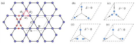
Figure 1: (a) Schematics for the kagome ferromagnet with lattice constant $a$. The NN vectors are labeled by $a_{i}$. Sublattices A, B, and C are placed at the corners of the triangles. Dzyaloshinskii-Moriya vectors are aligned normal to the lattice plane, and their directions (up and down) are represented by the symbols $\odot$ and $\otimes$, depending on the chirality of the triangles. The dashed lines represent a unit cell. (b)-(c) Strain is introduced by letting the sublattice far away ($\delta>0$) or closer ($\delta<0$).

Different topological phases are characterized by sets of Chern numbers $(C_{1},C_{2},C_{3})$ of the lower, middle and upper magnon bulk bands. A topological phase transition has been discovered by tuning $\delta$ [49]. Fig. 2(a) shows the magnon bulk bands along the high-symmetry directions ($\Gamma$-$K$-$M$-$\Gamma$) of the Brillouin zone. For $\delta=0$ the topological phase is $(-1,0,1)$ and for $\delta=0.1$ the topological phase is $(0,-1,1)$. A topological phase transition occurs at $\delta_{c}=0.05$, where the two magnon branches cross linearly at the $K$ point.

The DMI breaks $C_{6z}$ symmetry to $C_{3z}$, yet preserves the $C_{2x}$ symmetry. Then both of the LP and CP responses are forbidden. It is worthy noting that the breathing geometry preserves the $C_{3z}$ symmetry and breaks $C_{2x}$, hence all the CP responses are forbidden but the LP responses are allowed. In Fig. 2(b) we show the magnon spin photoconductivities $\eta^{xxx}$ of the allowed injection, rectification, and shift spin current in response of the LP light, varying with the lattice deformation. For $\delta=0$, the LP responses are zero owing to the $C_{2x}$ symmetry. As $\delta$ increases, finite LP responses appear as required by symmetry. The $(-1,0,1)$ phase and the $(0,-1,1)$ phase are separated by the critical points of phase transition represented by the dashed black lines. Remarkably, the injection spin current exhibits a peak and the rectification spin current develops a dip at the critical point; while the derivative of the shift spin current maximizes at the critical point. As for the Drude spin current, there is no such drastic change at the critical point, because the Drude spin current is exclusively determined by the group velocities and their derivatives, which is independent of the magnon topology. Thus it clearly indicates a topological phase transition that is also manifested as a plateau of the total LP photoconductivity at the critical point, which can serve as a prominent indicator to determine the topological phase transition in experiments.

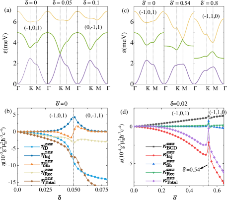
Figure 2: (a) Magnon band structures of a breathing kagome-lattice ferromagnet with different lattice deformation $\delta$. Considering that $\delta>0$ and $\delta<0$ are equivalent, only cases $\delta>0$ are plotted. (b) LP photoconductivities as a function of the lattice deformation. The critical point of phase transition is shown as vertical dashed line. (c) Magnon band structures of a breathing kagome-lattice ferromagnet in the presence of $\delta=0.02$ with different uniaxial strain $\delta^{\prime}$. The critical point is $\delta^{\prime}=0.54$. (d) The CP photoconductivities versus the uniaxial strain $\delta^{\prime}$, where the critical point of phase transition is shown as vertical dashed line. Parameters are set as $D=0.3$, $\hbar\Omega=0.2$, $k_{B}T=2$, $\Gamma=0.1$, and unit is meV.

As mentioned above, a breathing kagome-lattice ferromagnet preserves the $C_{3z}$ symmetry hence all the CP responses are forbidden. Now we consider an additional uniaxial strain along the $x$-axis breaking the $C_{3z}$ symmetry, for which the spins along the $x$-axis are pushing closer $\delta^{\prime}>0$ or further $\delta^{\prime}<0$, as shown in Figs. 1(d)-(e). The remaining point-group symmetry is $\sigma_{x}$, for which the CP responses are allowed. In the presence of this uniaxial strain $\delta^{\prime}$, the diagonal component $\mathcal{H}_{0}$ is modified as $\mathcal{H}_{0}=J\text{diag}(4,2(2+\delta^{\prime}),2(2+\delta^{\prime}))$. For $\mathcal{H}_{J}^{NN}$, only the $(1,2)$ and $(2,1)$ elements are changed to $\gamma_{2}^{\prime}=(1+\delta^{\prime})\gamma_{2}$ [51]. By increasing $\delta^{\prime}$ from zero, a topological phase transition occurs at the critical point $\delta_{c}^{\prime}=\frac{1}{2}[1-(D/J)^{2}]$, where the upper band and the middle band cross at the M point. In Fig. 2(c) we show the magnon bands along the high symmetry points for different $\delta^{\prime}$ but with fixed $\delta=0.02$ (and $D/J=0.2$). Similar to that in Ref. [51], a topological phase transition occurs when the system is tuned from the $(-1,0,1)$-phase to $(-1,1,0)$-phase by increasing $\delta^{\prime}$; while the critical point is found at $\delta_{c}^{\prime}=0.54$. In Fig. 2(d) we show the CP spin conductivities $\kappa^{xyx}_{s}$ as functions of $\delta^{\prime}$. One observes that all the four kinds of the CP responses change abruptly at $\delta^{\prime}=\delta_{c}^{\prime}$, as an indication of a topological magnon phase transition, which is a direct manifestation of the change of the topological properties such as the Berry curvature and the shift vector in momentum space.

The breathing kagome lattice has gained growing interest in the studies of the quantum spin liquid [52, 53, 54, 55, 50, 56]. It has been synthesized in the rare-earth based pyrochlore material $\mathrm{Ba_{3}Yb_{2}Zn_{5}5O_{11}}$ [57], as well as material $\mathrm{LiZn_{2}Mo_{3}O_{8}}$ [58]. Recently, a field-aligned ferromagnetic phase was experimentally observed in the centrosymmetric breathing kagome lattice $\mathrm{Gd_{3}Ru_{4}Al_{12}}$ [59], which makes it a potential candidate material.

To conclude, we have proposed the magnon spin photogalvanic effect and revealed the geometric origin in the AC phase accumulation. It gives a new mechanism for optical (electric) control of the magnon spin current. Armed with a perturbative theory that accounts for the interplay between electric field and magnon by introducing the dipole interaction, we identify five new mechanisms, such as the Drude, BCD, injection, shift, and the rectification spin current, and systematically studied these spin optical responses under the LP and CP light in collinear ferromagnet. Analytical formulas are derived and tabulated for convenience. On the basis of a symmetry classification, we predicted the presence of the spin photocurrent in the breathing kagome-lattice ferromagnet and showed that the magnon SPGV can act as an optical method to probe the topological phase transitions of quantum magnets. The generated magnon spin current can be detected via the inverse spin Hall effect (ISHE) [60, 61, 62]. Given the symmetry analysis, this study can be naturally extended to other materials by using the magnetic structure database MAGNDATA [63]. We believe that these results can stimulate further experimental explorations and broaden the research scope of magnon spintronics. Our proposal may be useful to manipulate magnon dynamics.

This work is supported by the National Key R&D Program of China (Grant No. No. 2022YFA1402802). It is also supported in part by the NSFC (Grants No. 11974348 and No. 11834014), and the Strategic Priority Research Program of CAS (Grants No. XDB28000000, and No. XDB33000000). Z.G.Z. is supported in part by the Training Program of Major Research plan of the National Natural Science Foundation of China (Grant No. 92165105), and CAS Project for Young Scientists in Basic ResearchGrant No. YSBR-057.

Supplemental Materials for “Magnon Spin Photogalvanic Effect in Collinear Ferromagnets”

This Supplemental Material consists of three sections. In Section I, we review linear spin-wave theory, which is the framework within which we derive the magnon SPGE. In Section II, we derive the perturbed magnon Hamiltonian in form of minimal coupling. A gauge transformation is presented in Section III to derived the dipole interaction. In Section IV we derive the magnon spin current operator. Then, we calculated the dc magnon spin photocurrent in Section V. Finally, in Section VI we give a symmetry analysis on the magnon spin photocurrent conductivities and make classification with the point-group symmetry and the combination with effective time-reversal symmetry.

I I. Linear spin-wave theory and magnon Hamiltonian

Here we rewrite the general two-body spin interaction Hamiltonian,

$$H=\frac{1}{2}\sum_{i,j}^{L}\sum_{n,m}^{N}\sum_{\alpha\beta}{S}^{\alpha}_{i,n}H^{\alpha\beta}_{nm}(i-j){S}^{\beta}_{j,m},$$ (S1)

By setting a global (reference) coordinates $(\hat{\bm{x}},\hat{\bm{y}},\hat{\bm{z}})$, the local coordinates (spherical coordinates) of each spin relate the global coordinate through

$$\bm{S}_{i,n}=R_{n}(\theta_{i},\phi_{i})\bm{S}_{0}$$ (S2)

The classical ground state is identified by treating the quantum mechanical spins operators as classical vectors and minimizing the classical ground-state energy. The magnons are the usual low-energy excitation in ordered magnets, which is considered via the Holstein-Primakoff transformation in local coordinates [64, 65]

$$S_{i,n}^{\theta}=\sqrt{\frac{S}{2}}(a_{i,n}+a_{i,n}^{\dagger}),\quad S_{i,n}^{\phi}=-i\sqrt{\frac{S}{2}}(a_{i,n}-a_{i,n}^{\dagger}),$$ (S3)

$$S_{i,n}^{r}=S-a_{i,n}^{\dagger}a_{i,n}.$$

and we obtain

$$\bm{S}_{i,n}^{\alpha}=\sqrt{\frac{S}{2}}\hat{\bm{u}}_{n}a_{i,n}+\sqrt{\frac{S}{2}}\hat{\bm{u}}_{n}^{*}a_{i,n}^{\dagger}+\hat{\bm{z}}_{n}(S-a_{i,n}^{\dagger}a_{i,n}),$$ (S4)

In which $\alpha=x,y,z$, the coefficients $\hat{\bm{u}}_{n}$ and $\hat{\bm{z}}_{n}$ are related to the relative rotation between the global and local coordinates, that are explicitly written as

$$\begin{pmatrix}u_{n}^{x}\\ u_{n}^{y}\\ u_{n}^{z}\end{pmatrix}=\begin{pmatrix}\cos{\theta_{n}}\cos{\phi_{n}}+i\sin{\phi_{n}}\\ \cos{\theta_{n}}\cos{\phi_{n}}-i\sin{\phi_{n}}\\ -\sin{\theta_{n}}\end{pmatrix},\quad\begin{pmatrix}z_{n}^{x}\\ z_{n}^{y}\\ z_{n}^{z}\end{pmatrix}=\begin{pmatrix}\sin{\theta_{n}}\cos{\phi_{n}}\\ \sin{\theta_{n}}\sin{\phi_{n}}\\ \cos{\theta_{n}}\end{pmatrix}.$$ (S5)

Expanding the coupling interaction, we obtain

$$S_{i,n}^{\alpha}S_{j,m}^{\beta}= \frac{1}{2}u_{n}^{\alpha*}a_{i,n}^{\dagger}(u_{m}^{\beta}a_{j,m}+u_{m}^{\beta*}a_{j,m}^{\dagger})+\frac{1}{2}u_{n}^{\alpha}a_{i,n}(u_{m}^{\beta*}a_{j,m}^{\dagger}+u_{m}^{\beta}a_{j,m})-z_{n}^{\alpha}z_{m}^{\beta}(a_{i,n}^{\dagger}a_{i,n}+a_{j,m}^{\dagger}a_{j,m}).$$ (S6)

By inserting Eq. (S6) into Eq. (S1), we have

$$H= \sum_{i,j,n,m}A_{nm}(i-j)a_{i,n}^{\dagger}a_{j,m}+\frac{1}{2}\sum_{i,j,n,m}\left[B_{nm}(i-j)a_{i,n}^{\dagger}a_{j,m}^{\dagger}+\text{h.c.}\right]+2\sum_{i,n,m}C_{nm}a_{i,n}^{\dagger}a_{i,n}.$$ (S7)

In which

$$A_{nm}(i-j)=\frac{\sqrt{S_{n}S_{m}}}{2}\sum_{\alpha\beta}u_{n}^{\alpha*}H_{nm}^{\alpha\beta}(i-j)u_{m}^{\beta},$$ (S8)

$$B_{nm}(i-j)=\frac{\sqrt{S_{n}S_{m}}}{2}\sum_{\alpha\beta}u_{n}^{\alpha*}H_{nm}^{\alpha\beta}(i-j)u_{m}^{\beta*},$$

$$C_{nm}=\delta_{nm}S_{l}\sum_{\alpha\beta}z_{n}^{\alpha}\sum_{j}\sum_{l}H_{nm}^{\alpha\beta}(i-j)z_{l}^{\beta}.$$

By transforming Eq. (S6) to the reciprocal space, there is

$$a_{i,n}=(1/\sqrt{L})\sum_{\bm{k}}\exp{[i\bm{k}\cdot(\bm{r}_{i}+\bm{t}_{n})]}a_{\bm{k},n},$$ (S9)

where $\bm{r}_{i}$ is the position of the $i$th unit cell and $\bm{t}_{m}$ is the relative vector of the $m$th sublattice. We have $H=\frac{1}{2}\sum_{\bm{k}}\Psi_{\bm{k}}^{\dagger}\mathcal{H}(\bm{k})\Psi_{\bm{k}}$, where

$$\mathcal{H}(\bm{k})=\begin{pmatrix}A(\bm{k})-C&B(\bm{k})\\ B^{\dagger}(\bm{k})&A^{T}(-\bm{k})-C\end{pmatrix}$$ (S10)

is a 2N$\times$2N bosonic Bogoliubov-de Gennes (BdG) Hamiltonian with the vector boson operator where $\Psi_{\bm{k}}^{\dagger}=(a_{{\bm{k}},1}^{\dagger},\cdots,a_{{\bm{k}},N}^{\dagger},a_{{-\bm{k}},1},\cdots,a_{{-\bm{k}},N})$, and the $N\times N$ block matrix is given by

$$A_{mn}(\bm{k})=\sum_{\alpha,\beta}u_{n}^{\alpha*}\left[\sum_{\bm{d}}e^{-i\bm{k}\cdot\bm{d}}H_{nm}^{\alpha\beta}(\bm{d})\right]u_{m}^{\beta},$$ (S11)

$$B_{mn}(\bm{k})=\sum_{\alpha,\beta}u_{n}^{\alpha*}\left[\sum_{\bm{d}}e^{-i\bm{k}\cdot\bm{d}}H_{nm}^{\alpha\beta}(\bm{d})\right]u_{m}^{\beta*},$$

$$C_{mn}=\delta_{mn}\sum_{\alpha,\beta}\sum_{l}z_{n}^{\alpha*}\left[\sum_{\bm{d}}H_{nl}^{\alpha\beta}(\bm{d})\right]z_{l}^{\beta}.$$

Where $\bm{d}=(\bm{r}_{i}+\bm{t}_{n})-(\bm{r}_{j}-\bm{t}_{m})$ is the difference vector between the $m$th and the $n$th spin. In deriving Eq. (S11) the relation

$$\sum_{\bm{k}}\sum_{n,m}A_{nm}(\bm{k})a_{\bm{k},n}^{\dagger}a_{\bm{k},m}=\sum_{\bm{k}}\sum_{n,m}A_{nm}^{T}(-\bm{k})a_{-\bm{k},n}a_{-\bm{k},m}^{\dagger}$$ (S12)

is used. For collinear ferromagnets, the Hamiltonian Eq. (S10) is block diagonal with identical block which can be reduced to $H=\sum_{\bm{k}}\Psi_{\bm{k}}\mathcal{H}_{\bm{k}}\Psi_{\bm{k}}$ with $\mathcal{H}_{\bm{k}}=(A_{\bm{k}}-C)$ and $\Psi_{\bm{k}}^{\dagger}=(a_{\bm{k},1}^{\dagger},\cdots,a_{\bm{k},N}^{\dagger})$.

In general the bosonic Hamiltonian Eq. (S10) does not conserve the particle number, for example, the ferromagnets with elliptical magnons (where an anisotropy deforms the formerly circular precession) or in non-ferromagnets. And the Hamiltonian is diagonalized with the Bogoliubov transformation

$$U^{\dagger}_{\bm{k}}\mathcal{H}_{\bm{k}}U_{\bm{k}}=\mathcal{E}_{\bm{k}},$$ (S13)

which satisfies $U_{\bm{k}}\Sigma_{z}U_{\bm{k}}^{\dagger}=\Sigma_{z}$, where the diagonal matrix $\Sigma_{z}=\text{diag}(1,1,\cdots,-1,-1,\cdots)$ with $N$ positive ones and $N$ minus ones along the diagonal. The vector boson operator transforms as $\Psi_{\bm{k}}=U_{\bm{k}}\Phi_{\bm{k}}$. The $m$th column vector encoded in the matrix $U_{\bm{k}}$ stands for the (periodic part of) Bloch wave function for the $m$th magnon band [66]. Noting that $\Phi_{\bm{k}}$ does not satisfy the commutation relation of Bosons. Instead it satisfies

$$[\Phi_{\bm{k}},\Phi_{\bm{k}^{\prime}}^{\dagger}]=\Sigma_{z}\delta_{\bm{k},\bm{k}^{\prime}}.$$ (S14)

The equilibrium density matrix in band space is given as

$$\rho_{\bm{k}m}^{(0)}(t)\equiv\langle(\Phi_{\bm{k}}^{\dagger})_{m}(t)(\Phi_{\bm{k}})_{m}(t)\rangle_{0}.$$ (S15)

Where the subscript “0” denotes the equilibrium state, and $(\Phi_{\bm{k}}^{\dagger})_{m}$ is the $m$th element of the vector $\Phi_{\bm{k}}^{\dagger}$. For later convenience, we write $(\Phi_{\bm{k}}^{\dagger})_{m}$ as $\Phi_{\bm{k}m}^{\dagger}$. By using of Eq. (S14), one obtains

$$\rho_{\bm{k}m}=\begin{cases}g(\mathcal{E}_{\bm{k}m}),&[\Phi_{\bm{k}m},\Phi_{\bm{k}m}^{\dagger}]=1\\ -g(-\mathcal{E}_{\bm{k}m}),&[\Phi_{\bm{k}m},\Phi_{\bm{k}m}^{\dagger}]=-1,\end{cases}$$ (S16)

where $g(\mathcal{E}_{\bm{k}m})$ is the Bose-Einstein distribution $g(\mathcal{E}_{\bm{k}m})=1/(e^{\beta\mathcal{E}_{\bm{k}m}}-1)$. It is convenient to introduce the matrix $\varepsilon_{\bm{k}}$ [67]:

$$\varepsilon_{\bm{k}}=\Sigma_{z}\mathcal{E}_{\bm{k}}=U_{\bm{k}}^{-1}\Sigma_{z}\mathcal{H}_{\bm{k}}U_{\bm{k}},$$ (S17)

and the density matrix is simplified as $\rho_{\bm{k}m}=\Sigma_{z,mm}g(\varepsilon_{\bm{k}m})$. For general operator, with the Bogolyubov’s representation, it transforms

$$\hat{\mathcal{O}}=\sum_{\bm{k}}\Psi_{\bm{k}}^{\dagger}\mathcal{O}_{\bm{k}}\Psi_{\bm{k}}=\sum_{\bm{k}}\Phi_{\bm{k}}^{\dagger}\Sigma_{z}\tilde{\mathcal{O}}_{\bm{k}}\Phi_{\bm{k}}$$ (S18)

with the definition $\tilde{\mathcal{O}}_{\bm{k}}=U_{\bm{k}}^{-1}\Sigma_{z}\mathcal{O}U_{\bm{k}}$.

II II. Perturbation of electric field in form of minimal coupling

Now we consider the the AC effect. In Eq. (S6) the first two terms describe the magnon hopping. In the presence of electric field, the magnon acquires a phase while travelling between the $m$th and the $n$th spin on the $i$th and $j$th site, which is given by

$$\theta_{in,jm}=-\frac{g\mu_{B}}{\hbar c^{2}}\int_{\bm{r}_{i,n}}^{\bm{r}_{j,m}}(\bm{E}(t)\times\hat{\bm{e}}_{n})\cdot d\bm{r},$$ (S19)

The coupling interaction is modified as

$$S_{i,n}^{\alpha}S_{j,m}^{\beta}= \frac{1}{2}U_{n}^{\alpha*}a_{i,n}^{\dagger}(U_{m}^{\beta}a_{j,m}+U_{m}^{\beta*}a_{j,m}^{\dagger})e^{i\theta_{in,jm}}+\frac{1}{2}U_{n}^{\alpha}a_{i,n}(U_{m}^{\beta*}a_{j,m}^{\dagger}+U_{m}^{\beta}a_{j,m})e^{-i\theta_{in,jm}}$$ (S20)

$$-V_{n}^{\alpha}V_{m}^{\beta}(a_{i,n}^{\dagger}a_{i,n}+a_{j,m}^{\dagger}a_{j,m}).$$

Supposing that the scale of the spacial variance of $\bm{E}$ is much larger than lattice constant and introducing the effective vector potential $\bm{A}^{E}_{n}=\frac{1}{c}\bm{E}\times\hat{\bm{e}}_{n}$, one obtains

$$\theta_{in,jm}= \frac{g\mu_{B}}{\hbar c}\bm{A}^{E}_{n}\cdot\bm{d},$$ (S21)

Following the same procedure, we have

$$A_{nm}(\bm{k})\rightarrow A_{nm}(\bm{k}-\frac{g\mu_{B}}{\hbar c}\bm{A}^{E}_{n}),$$ (S22)

$$B_{nm}(\bm{k})\rightarrow B_{nm}(\bm{k}-\frac{g\mu_{B}}{\hbar c}\bm{A}^{E}_{n}).$$

While the matrix $C_{nm}$ is unchanged since for which the magnon hopping is not involved.

Now we consider two special cases: the collinear ferromagnet and collinear antiferromagnet.

II.1 Collinear ferromagnet

For ferromagnet due to the absence of the magnon paring $a^{\dagger}_{i,n}a^{\dagger}_{j,m}$ and $a_{i,n}a_{j,m}$, the 2N dimensional basis is reduce to N dimensional $\Psi_{\bm{k}}^{\dagger}=(a_{\bm{k},1}^{\dagger},\cdots a_{\bm{k},N}^{\dagger})$. Accordingly, the Hamiltonian Eq. (S10) is reduced to $\mathcal{H}_{\bm{k}}=A(\bm{k})-C$. It is obvious that the global coordinates is same to the local coordinate for each spin, which can be chosen as that where $z$-direction is identical to the magnetization direction. With this assignment, the magnetic moment of magnon is $-\hbar\hat{\bm{e}}_{z}$, and the effective vector potential is $\bm{A}^{E}_{n}=\bm{A}^{E}=\frac{1}{c}\bm{E}\times\hat{\bm{e}}_{z}$. Consequently, the kernal Hamiltonian becomes $\mathcal{H}(\bm{k})=A(\bm{k}-\frac{g\mu_{B}}{\hbar c}\bm{A}^{E})-C$.

II.2 Collinear antiferromagnet

To be concrete, we consider a collinear antiferromagnet honeycomb lattice that has two spins in a unit cell, with the Hamiltonian given by

$$H=J_{1}\sum_{\langle i,j\rangle}\bm{S}_{i}\cdot\bm{S}_{j}+D\sum_{\langle\langle ij\rangle\rangle}\xi_{ij}\hat{\bm{z}}\cdot\bm{S}_{i}\times\bm{S}_{j}+K\sum_{i}S_{iz}^{2}.$$ (S23)

In which $J_{1}>0$ is the antiferromagnetic exchange interaction, $D$ is the DMI interaction along the $z$ direction, and $\xi_{ij}=1(-1)$ when $\bm{S}_{i}$ and $\bm{S}_{j}$ are arranged in a counterclockwise (clockwise) manner. $K<0$ is the easy axis anisotropy. One can choose the local coordinates of 1st spin of the unit cell as the global coordinates, while the local coordinates of the 2nd spin is obtained by a $pi$ rotation about the $x$-axis or $y$-axis of the global coordinates. subsequently, the HP transformation is preformed as

$$\bm{S}_{i,1}^{\alpha}=\sqrt{\frac{S}{2}}\hat{\bm{u}}_{1}a_{i,1}+\sqrt{\frac{S}{2}}\hat{\bm{u}}_{1}^{*}a_{i,1}^{\dagger}+\hat{\bm{z}}_{1}(S-a_{i,1}^{\dagger}a_{i,1}),$$ (S24)

$$\bm{S}_{i,2}^{\alpha}=\sqrt{\frac{S}{2}}\hat{\bm{u}}_{2}a_{i,2}+\sqrt{\frac{S}{2}}\hat{\bm{u}}_{2}^{*}a_{i,2}^{\dagger}+\hat{\bm{z}}_{2}(S-a_{i,2}^{\dagger}a_{i,2}),$$

In which

$$\begin{pmatrix}u_{1}^{x}\\ u_{1}^{y}\\ u_{1}^{z}\end{pmatrix}=\begin{pmatrix}1\\ -i\\ 0\end{pmatrix},\quad\begin{pmatrix}z_{1}^{x}\\ z_{1}^{y}\\ z_{1}^{z}\end{pmatrix}=\begin{pmatrix}0\\ 0\\ 1\end{pmatrix},$$ (S25)

$$\begin{pmatrix}u_{2}^{x}\\ u_{2}^{y}\\ u_{2}^{z}\end{pmatrix}=\begin{pmatrix}1\\ i\\ 0\end{pmatrix},\quad\begin{pmatrix}z_{2}^{x}\\ z_{2}^{y}\\ z_{2}^{z}\end{pmatrix}=\begin{pmatrix}0\\ 0\\ -1\end{pmatrix}.$$

Therefore the magnon Hamiltonian is $H=H^{J}+H^{D}+H^{K}$ with

$$H^{J}= J_{1}S\sum_{\langle i,j\rangle}(a_{i,1}a_{j,2}+a_{i,1}^{\dagger}a_{j,2}^{\dagger}),$$ (S26)

$$H^{D}= -\sum_{\langle\langle i,j\rangle\rangle}iD_{2}S(a_{i,1}^{\dagger}a_{j,1}-a_{j,1}^{\dagger}a_{i,1}-a_{i,2}^{\dagger}a_{j,2}+a_{j,2}^{\dagger}a_{i,2}),$$

$$H^{K}= \sum_{i}(3J_{1}-K)S(a_{i,1}^{\dagger}a_{i,1}+a_{i,2}^{\dagger}a_{i,2}).$$

The operator $a_{i,1}$ ($a_{i,1}^{\dagger}$) annihilates (creates) a magnon with magnetic moment $-\hbar\hat{\bm{e}}_{z}$, and the effective vector potential is given as $\bm{A}_{n}^{E}=\bm{A}^{E}=\frac{1}{c}\bm{E}\times\bm{e}_{z}$. The magnon Hamiltonian in the presence of the electric field is written as

$$H^{J}= J_{1}S\sum_{i,\delta}(a_{i,1}a_{i+\delta,2}e^{i\theta_{r_{i},r_{i}+\delta}^{N}}+\text{h.c.}),$$ (S27)

$$H^{D}= -\sum_{i,\vartheta}iD_{2}S(a_{i,1}^{\dagger}a_{i+\vartheta,1}e^{-i\theta_{r_{i},r_{i}+\vartheta}^{NN}}-a_{i,2}^{\dagger}a_{i+\vartheta,2}e^{i\theta_{r_{i},r_{i}+\vartheta}^{NN}}+\text{h.c.}),$$

where the phase accumulated along the nearest (second-nearest) neighbor hopping is given as

$$\theta_{r_{i},r_{i}+\delta}^{N}= -\frac{g\mu_{B}}{\hbar c^{2}}\int_{r_{i}}^{r_{i}+\delta}(\bm{E}(t)\times\bm{e}_{z})\cdot d\bm{r},$$ (S28)

$$\theta_{r_{i},r_{i}+\vartheta}^{NN}= -\frac{g\mu_{B}}{\hbar c^{2}}\int_{r_{i}}^{r_{i}+\vartheta}(\bm{E}(t)\times\bm{e}_{z})\cdot d\bm{r}.$$

Supposing that the scale of the spacial variance of $\bm{E}$ is much larger than lattice constant one obtains

$$\theta_{r_{i},r_{i}+\delta}^{N}= \frac{g\mu_{B}}{\hbar c}\bm{A}^{E}\cdot\bm{\delta},$$ (S29)

$$\theta_{r_{i},r_{i}+\vartheta}^{NN}= \frac{g\mu_{B}}{\hbar c}\bm{A}^{E}\cdot\bm{\vartheta}.$$

Making use of the Fourier transformation Eq. (S9), one directly obtains $H=\sum_{\bm{k}}\Psi_{\bm{k}}^{\dagger}\mathcal{H}(\bm{k}-\frac{g\mu_{B}}{\hbar c}\bm{A})\Psi_{\bm{k}}$, with the Nambu basis given by $\Psi_{\bm{k}}^{\dagger}=(a_{\bm{k},1}^{\dagger},a_{\bm{k},2}^{\dagger},a_{-\bm{k},1},a_{-\bm{k},2})$. In which $A_{mn}(\bm{k})-C_{mn}$ is diagonal with $A_{11(22)}(\bm{k})-C_{11(22)}=\frac{S}{2}\left[3J_{1}-K(2S-1)/S\pm D\sum_{\bm{\delta}}2\sin(\bm{k}\cdot\bm{\delta})\right]$, and $B_{mn}(\bm{k})$ is non-diagonal with $B_{12}(\bm{k})=B_{21}^{*}(\bm{k})=\frac{S}{2}\left[\sum_{\bm{\vartheta}}\exp{(i\bm{k}\cdot\bm{\vartheta})}\right]$.

III III. Gauge transformation and dipole interaction

In this section we give a gauge transformation to derive perturbed Hamiltonian in form of a dipole interaction. The single-particle Hamiltonian and the Bloch Hamiltonian satisfy

$$\mathcal{H}_{0}(-i\bm{\nabla},\bm{r})=e^{i\bm{k}\cdot\bm{r}}\mathcal{H}_{0}(\bm{k})e^{-i\bm{k}\cdot\bm{r}}.$$ (S30)

According to Sec. II, the perturbed Hamiltonian is written as

$$\mathcal{H}_{A}=\mathcal{H}_{0}\left(-i\bm{\nabla}+\frac{g\mu_{B}}{\hbar c}\bm{A},\bm{r}\right).$$ (S31)

The time-dependent Schördinger equation is

$$i\hbar\frac{\partial\left|\psi(\bm{r},t)\right>}{\partial t}=\mathcal{H}_{A}\left|\psi(\bm{r},t)\right>.$$ (S32)

There is freedom of choice of the phase of the wave functions. A unitary gauge transformation of $\left|\psi(\bm{r},t)\right>$ takes the form

$$\left|\psi^{\prime}(\bm{r},t)\right>=\mathcal{U}(t)\left|\psi(\bm{r},t)\right>,$$ (S33)

The time-dependent Schördinger equation transforms as

$$i\hbar\frac{\partial\left|\psi^{\prime}(\bm{r},t)\right>}{\partial t}=\left[\mathcal{U}\mathcal{H}_{A}\mathcal{U}^{\dagger}\left|\psi(\bm{r},t)\right>+i\hbar\frac{\partial\mathcal{U}(t)}{\partial t}\mathcal{U}^{\dagger}(t)\right]\left|\psi^{\prime}(\bm{r},t)\right>.$$ (S34)

If the unitary transformation is chosen as $\mathcal{U}(t)=e^{i\mathcal{S}(t)}$ with

$$\mathcal{S}(t)=\frac{g\mu_{B}}{\hbar c}\bm{A}(t)\cdot\bm{r}.$$ (S35)

For the first term in the r.h.s. of Eq. (S34), by use of the Baker-Campbell-Hausdorff identity

$$e^{i\mathcal{S}}\mathcal{H}_{A}e^{-i\mathcal{S}}= \mathcal{H}+i[\mathcal{S},\mathcal{H}_{A}]-\frac{1}{2}[\mathcal{S},[\mathcal{S},\mathcal{H}_{A}]]...+\frac{i^{n}}{n!}[\mathcal{S},...,[\mathcal{S},\mathcal{H}_{A}]]+...,$$ (S36)

it is obtained that

$$\mathcal{U}(t)\mathcal{H}_{A}\mathcal{U}^{\dagger}(t)=\mathcal{H}_{0}.$$ (S37)

For the second term in the r.h.s. of Eq. (S34), by introducing the effective electric field $\tilde{\bm{E}}=-\partial_{t}\bm{A}$, it is straightforward to show that

$$i\hbar\frac{\partial\mathcal{U}(t)}{\partial t}\mathcal{U}^{\dagger}(t)=\frac{g\mu_{B}}{c}\tilde{\bm{E}}(t)\cdot\bm{r}.$$ (S38)

Then the Hamiltonian in velocity gauge transform to

$$\mathcal{H}_{E}(t)=\mathcal{H}_{0}\left(\bm{k}\right)+\frac{g\mu_{B}}{c}\tilde{\bm{E}}(t)\cdot\bm{r}.$$ (S39)

IV IV. Magnon spin current

Now we define the magnon spin current. Because the $z$ component of the total spin is conserved, the local magnon spin density (LMSD) is $n_{z}(\bm{r}_{i})=\hbar\sum_{m}\bm{z}_{m}a_{i,m}^{\dagger}a_{i,m}$ satisfying the continuity equation. The Fourier transformation of the LMSD is written as

$$n_{z}(\bm{r}_{i})=\frac{\hbar}{N}\sum_{\bm{k}\bm{q}m}\bm{z}_{m}e^{-i\bm{q}\cdot(\bm{r}_{i}+\bm{t}_{m})}a_{\bm{k}+\bm{q},m}^{\dagger}a_{\bm{k},m}.$$ (S40)

The Heisenberg equation of motion for $a_{\bm{k},m}$ is used to derive the equation of motion for $n_{z}(\bm{r}_{i})$:

$$\dot{a}_{\bm{k},m}= \frac{1}{i\hbar}[a_{\bm{k},m},H]$$ (S41)

$$= \frac{1}{i\hbar}\sum_{n}(A_{\bm{k},mn}a_{\bm{k},n}+A_{\bm{k},mn}a_{\bm{k},n}+B_{\bm{k},mn}^{*}a_{-\bm{k},n}),$$

$$= \frac{1}{i\hbar}\sum_{n}(2A_{\bm{k},mn}a_{\bm{k},n}+B_{\bm{k},mn}a_{-\bm{k},n}^{\dagger}+B_{-\bm{k},nm}a_{-\bm{k},n}^{\dagger}),$$

where $H$ is given by Eq. (S10), and we obtain:

$$\frac{\partial n_{z}(\bm{r}_{i})}{\partial t}= \frac{1}{iN}\sum_{\bm{k}\bm{q}mn}e^{-i\bm{q}\cdot\bm{r}_{i,m}}\bm{z}_{m}\left[-\left(2A_{\bm{k+q},nm}a_{\bm{k+q},n}^{\dagger}+(B^{*}_{\bm{k+q},mn}+B^{*}_{\bm{-k-q},nm})a_{-\bm{k-q},n}^{\dagger}\right)a_{\bm{k},m}\right.$$ (S42)

$$\left.+a_{\bm{k+q},m}^{\dagger}\left(2A_{\bm{k},mn}a_{\bm{k},n}+(B_{\bm{k},mn}+B_{-\bm{k},nm})a_{-\bm{k},n}^{\dagger}\right)\right].$$

In the case $\sum\bm{\delta}=0$ and assuming the long-wavelength limit $\bm{q}\rightarrow 0$, the magnon spin current is obtained by use of the continuity equation $\partial n_{z\bm{q}}/\partial t+i\bm{q}\cdot\bm{J}_{s,z}=0$, which is given as

$$\bm{J}_{s,z}= \hbar\sum_{\bm{k}mn}\bm{z}_{m}\left(\frac{\partial A_{\bm{k},mn}}{\partial\bm{k}}a_{\bm{k},m}^{\dagger}a_{\bm{k},n}+\frac{\partial A_{-\bm{k},nm}}{\partial\bm{k}}a_{-\bm{k},m}a_{-\bm{k},n}^{\dagger}+\frac{\partial B_{\bm{k},mn}}{\partial\bm{k}}a_{\bm{k},m}^{\dagger}a_{-\bm{k},n}^{\dagger}+\frac{\partial B_{\bm{k},nm}^{*}}{\partial\bm{k}}a_{-\bm{k},m}a_{\bm{k},n}\right)$$ (S43)

$$= \hbar\sum_{\bm{k}}\Psi_{\bm{k}}^{\dagger}\mathcal{Z}\frac{\partial\mathcal{H}_{\bm{k}}}{\partial\bm{k}}\Psi_{\bm{k}}.$$

In Eq. (S43) we define the diagonal matrix $\mathcal{Z}$

$$\mathcal{Z}=\text{diag}(z_{1},\cdots,z_{m},z_{1},\cdots,z_{m}).$$ (S44)

Making use of Eq. (S18), we have

$$\bm{J}_{s,z}=\hbar\sum_{\bm{k}}\Phi_{\bm{k}}^{\dagger}\Sigma_{z}\frac{\widetilde{\partial\mathcal{Z}\mathcal{H}_{\bm{k}}}}{\partial\bm{k}}\Phi_{\bm{k}}.$$ (S45)

It is found that

$$\frac{\widetilde{\partial\mathcal{Z}\mathcal{H}_{\bm{k}}}}{\partial\bm{k}}=\frac{\partial\widetilde{\mathcal{Z}\mathcal{H}}_{\bm{k}}}{\partial\bm{k}}-\widetilde{\mathcal{Z}\mathcal{H}}_{\bm{k}}U_{\bm{k}}^{-1}\frac{\partial U_{\bm{k}}}{\partial\bm{k}}-\frac{\partial U_{\bm{k}}^{-1}}{\partial\bm{k}}U_{\bm{k}}\widetilde{\mathcal{Z}\mathcal{H}}_{\bm{k}},$$ (S46)

and we obtain

$$\bm{J}_{s,z}=\hbar\sum_{\bm{k}}\Phi_{\bm{k}}^{\dagger}\Sigma_{z}\left(\frac{\partial\widetilde{\mathcal{Z}\mathcal{H}_{\bm{k}}}}{\partial\bm{k}}-i[\bm{\mathcal{A}}_{\bm{k}},\widetilde{\mathcal{Z}\mathcal{H}_{\bm{k}}}]\right)\Phi_{\bm{k}},$$ (S47)

where the Berry connection is defined by

$$\bm{\mathcal{A}}_{\bm{k}}=iU_{\bm{k}}^{-1}\frac{\partial U_{\bm{k}}}{\partial\bm{k}}=i\Sigma_{z}U_{\bm{k}}^{\dagger}\Sigma_{z}\frac{\partial U_{\bm{k}}}{\partial\bm{k}}.$$ (S48)

Noting that the Berry connection given in Eq. (S48) is different from $iU_{\bm{k}}^{\dagger}\frac{\partial U_{\bm{k}}}{\partial\bm{k}}$. This is because that the Bogoliubov transformation is generally not unitary [68].

For collinear ferromagnets, owing to the reduction of 2N dimensional basis to the N dimensional the basis $\Psi_{\bm{k}}^{\dagger}=(a_{\bm{k},1}^{\dagger},\cdots,a_{\bm{k},N}^{\dagger})$, the direction matrix $\mathcal{Z}$ in Eq. (S44) becomes a unit matrix and the magnon spin current operator in Eq. (S47) becomes

$$\bm{J}_{s}=\hbar\sum_{\bm{k}}\Phi_{\bm{k}}^{\dagger}\left(\frac{\partial{\mathcal{H}_{\bm{k}}}}{\partial\bm{k}}-i[\bm{\mathcal{A}}_{\bm{k}},{\mathcal{H}_{\bm{k}}}]\right)\Phi_{\bm{k}}.$$ (S49)

V V. Magnon spin photocurrent in collinear ferromagnets

In this section we derive the equations of motion for the magnon density matrix in the presence of the AC phase induced by the electric field of light. A similar method for electron second-order optical responses is used to calculate the electric bulk photogalvanic effect [34, 35]. We give the formalism of nonlinear responses for the magnon spin photocurrent by standard perturbation technique. According to Eq. (9), the recursion equation can be rewritten as

$$\rho_{mn}^{(n+1)}(\omega)= \frac{g\mu_{B}}{\hbar c^{2}}d_{mn}(\omega)\int\frac{d\omega_{1}}{2\pi}\omega_{1}\epsilon^{\alpha_{1}z\beta}E^{\alpha_{1}}D^{\beta}[\rho^{(n)}(\omega-\omega_{1})]_{mn},$$ (S50)

where $\epsilon^{\alpha_{1}z\beta}$ the Levi-Civita symbol, and summation is implied over repeated spatial indices. In deriving the second-order reduced density matrix, it can be divided into terms originating from the intraband (i) and interband (e) components of $\mathcal{D}_{\text{opt}}$ operator:

$$\rho^{(2)}_{mn}(\omega)= \nu_{c}\sum_{X}\int\frac{d\omega_{1}d\omega_{2}}{(2\pi)^{2}}{\omega_{1}\omega_{2}}E^{\alpha_{1}}(\omega_{1})E^{\alpha_{2}}(\omega_{2})\epsilon^{\alpha_{1}z\beta}\epsilon^{\alpha_{2}z\gamma}\varrho^{X,\beta\gamma}_{mn}(\omega_{1},\omega_{2}),$$ (S51)

with the constant $\frac{g^{2}\mu_{B}^{2}}{\hbar^{2}c^{4}}$ is noted as $\nu_{c}$. Then, the contribution of each term in Eq. (S51) to the spin photoconductivities are noted as $\sigma_{X}^{\alpha\alpha_{1}\alpha_{2}}$ for $X=$ ii, ie, ei and ee. Keeping in mind that the energy conservation $\omega=\omega_{1}+\omega_{2}$ is always satisfied, the expressions for each term are obtained as

$$\varrho^{\text{ii},\beta\gamma}_{mn}(\omega_{1},\omega_{2})= -d_{mn}(\omega)d_{mn}(\omega_{2})(\partial^{\beta}\partial^{\gamma}g_{m})\delta_{mn},$$ (S52)

$$\varrho^{\text{ei},\beta\gamma}_{mn}(\omega_{1},\omega_{2})= -id_{mn}(\omega)d_{mm}(\omega_{2})\mathcal{A}_{mn}^{\gamma}\partial^{\beta}g_{nm},$$

$$\varrho^{\text{ie},\beta\gamma}_{mn}(\omega_{1},\omega_{2})= -id_{mn}(\omega)\left(\partial^{\gamma}\left[d_{mn}(\omega_{2})\mathcal{A}^{\beta}_{mn}g_{nm}\right]-i(\mathcal{A}^{\gamma}_{mm}-\mathcal{A}^{\gamma}_{nn})\left[d_{mn}(\omega_{2})\mathcal{A}^{\beta}_{mn}g_{nm}\right]\right),$$

$$\varrho^{\text{ee},\beta\gamma}_{mn}(\omega_{1},\omega_{2})= \sum_{p\neq m,n}d_{mn}(\omega)\left[\mathcal{A}_{mp}^{\gamma}d_{pn}(\omega_{2})\mathcal{A}_{pn}^{\beta}g_{np}-\mathcal{A}_{pn}^{\gamma}d_{mp}(\omega_{2})\mathcal{A}_{mp}^{\beta}g_{pm}\right].$$

Where we define $g_{mn}=g_{m}-g_{n}$. Note that $\varrho^{ii}$ and $\varrho^{ei}$ include the derivative to the Bose-Einstein distribution. Together with Eq. (S47) and Eq. (S52), the second-order magnon spin current is given as

$$J^{(2),\alpha}_{s}(\omega_{1},\omega_{2})=\sum_{X}E^{\beta}(\omega_{1})E^{\gamma}(\omega_{2})\chi_{X}^{\alpha\beta\gamma}(\omega_{1},\omega_{2}),$$ (S53)

with

$$\chi^{\alpha\alpha_{1}\alpha_{2}}_{\text{ii}}= -\frac{\nu_{c}}{2}\int[d\bm{k}]\sum_{m}\epsilon^{\alpha_{1}z\beta}\epsilon^{\alpha_{2}z\gamma}{\omega_{1}\omega_{2}}J_{s,mm}^{\alpha}d_{mm}(\omega_{2})d_{mm}(\omega)\partial^{\beta}\partial^{\gamma}g_{m}+[(\alpha_{1},\omega_{1})\leftrightarrow(\alpha_{2},\omega_{2})],$$ (S54)

$$\chi^{\alpha\alpha_{1}\alpha_{2}}_{\text{ei}}= -\frac{\nu_{c}}{2}\int[d\bm{k}]\sum_{m,n}i\epsilon^{\alpha_{1}z\beta}\epsilon^{\alpha_{2}z\gamma}{\omega_{1}\omega_{2}}J_{s,mn}^{\alpha}d_{nm}(\omega)d_{mm}(\omega_{2})\mathcal{A}_{nm}^{\gamma}\partial^{\beta}g_{nm}+[(\alpha_{1},\omega_{1})\leftrightarrow(\alpha_{2},\omega_{2})],$$ (S55)

$$\chi^{\alpha\alpha_{1}\alpha_{2}}_{\text{ie}}= -\frac{\nu_{c}}{2}\int[d\bm{k}]\sum_{m,n}i\epsilon^{\alpha_{1}z\beta}\epsilon^{\alpha_{2}z\gamma}{\omega_{1}\omega_{2}}J_{s,mn}^{\alpha}d_{nm}(\omega)\left(\partial^{\beta}\left[d_{nm}(\omega_{2})\mathcal{A}^{\gamma}_{nm}g_{nm}\right]-i(\mathcal{A}^{\beta}_{nn}-\mathcal{A}^{\beta}_{mm})\right.$$

$$\left.\times\left[d_{nm}(\omega_{2})\mathcal{A}^{\gamma}_{nm}g_{nm}\right]\right)+[(\alpha_{1},\omega_{1})\leftrightarrow(\alpha_{2},\omega_{2})],$$ (S56)

$$\chi^{\alpha\alpha_{1}\alpha_{2}}_{\text{ee}}= \frac{\nu_{c}}{2}\int[d\bm{k}]\sum_{m,n,p}\epsilon^{\alpha_{1}z\beta}\epsilon^{\alpha_{2}z\gamma}{\omega_{1}\omega_{2}}J_{s,mn}^{\alpha}d_{nm}(\omega)\left[d_{pm}(\omega_{2})\mathcal{A}_{np}^{\beta}\mathcal{A}_{pm}^{\gamma}g_{mp}-d_{np}(\omega_{2})\mathcal{A}_{pm}^{\beta}\mathcal{A}_{np}^{\gamma}g_{pn}\right]$$

$$+[(\alpha_{1},\omega_{1})\leftrightarrow(\alpha_{2},\omega_{2})].$$ (S57)

Note that the conductivity tensors are symmetrize by the indices and frequencies of electric fields. This is because the physical observables should not be affected by an arbitrary permutation of applied external fields, that is, the conductivity tensor has intrinsic permutation symmetry [34, 69]. It is clearly seen that the magnon photocurrent is quite different from the case of charge photocurrent. For the magnon photocurrent the electric field is restricted into the plane perpendicular to the axis of the magnon spin, while for the charge case the direction of the electric field can be arbitrary.

V.1 Drude spin current

According to Eq. (S54), $\chi^{\alpha\alpha_{1}\alpha_{2}}_{\text{ii}}$ only involves the intraband contribution, which is given by

$$\chi^{\alpha\alpha_{1}\alpha_{2}}_{\text{ii}}= -\lim_{\omega\rightarrow 0}\frac{\nu_{c}}{2\hbar^{2}\omega}\int[d\bm{k}]\sum_{m}\left(\epsilon^{\alpha_{1}z\beta}\epsilon^{\alpha_{2}z\gamma}\frac{1}{-\Omega}+\epsilon^{\alpha_{2}z\beta}\epsilon^{\alpha_{1}z\gamma}\frac{1}{\omega+\Omega}\right)\Omega(\omega+\Omega)J_{s,mm}^{\alpha}\partial^{\beta}\partial^{\gamma}g_{m}.$$ (S58)

It describes the drift movement of magnons driving by the optical field, and is noted as the Drude contribution. Following the definitions

$$\eta^{\alpha\alpha_{1}\alpha_{2}}=\frac{1}{2}\text{Re}(\chi^{\alpha\alpha_{1}\alpha_{2}}+\chi^{\alpha\alpha_{2}\alpha_{1}}),$$ (S59)

$$\kappa^{\alpha\alpha_{1}\alpha_{2}}=\frac{1}{2}\text{Im}(\chi^{\alpha\alpha_{1}\alpha_{2}}-\chi^{\alpha\alpha_{2}\alpha_{1}}),$$

we obtain the LP spin photocurrent conductivity

$$\eta^{\alpha\alpha_{1}\alpha_{2}}_{\text{D}}=\frac{\nu_{c}}{2\hbar^{2}}\int[d\bm{k}]\sum_{m}\left(\epsilon^{\alpha_{1}z\beta}\epsilon^{\alpha_{2}z\gamma}+\epsilon^{\alpha_{2}z\beta}\epsilon^{\alpha_{1}z\gamma}\right)v_{m}^{\alpha}\partial^{\beta}\partial^{\gamma}g_{m}.$$ (S60)

In Eq. (S58) we use the relation $J_{s,mm}^{\alpha}=\hbar v_{m}$ with $v_{m}=\frac{1}{\hbar}\partial^{\alpha}\varepsilon_{m}$ being the group velocity. To simplify the formulas, we define the symmetric combination of the Levi-Civita symbols as

$$E_{S}^{\alpha_{1}\alpha_{2}\beta\gamma}=\epsilon^{\alpha_{1}z\beta}\epsilon^{\alpha_{2}z\gamma}+\epsilon^{\alpha_{2}z\beta}\epsilon^{\alpha_{1}z\gamma}$$ (S61)

and the antisymmetric combination one as

$$E_{A}^{\alpha_{1}\alpha_{2}\beta\gamma}=\epsilon^{\alpha_{1}z\beta}\epsilon^{\alpha_{2}z\gamma}-\epsilon^{\alpha_{2}z\beta}\epsilon^{\alpha_{1}z\gamma}.$$ (S62)

and we have

$$\eta^{\alpha\alpha_{1}\alpha_{2}}_{\text{D}}= \frac{\nu_{c}}{2\hbar}\int[d\bm{k}]\sum_{m}E_{S}^{\alpha_{1}\alpha_{2}\beta\gamma}v_{m}^{\alpha}\partial^{\beta}\partial^{\gamma}g_{m}.$$ (S63)

Note that the integrand $v_{m}^{\alpha}\partial^{\beta}\partial^{\gamma}g_{m}$ in Eq. (S63) is symmetric by exchanging the external field indices $\beta$ and $\gamma$, hence $E_{S}^{\alpha_{1}\alpha_{2}\beta\gamma}=2$ for $\alpha_{1}=\alpha_{2}$ while $E_{S}^{\alpha_{1}\alpha_{2}\beta\gamma}=-2$ for $\alpha_{1}\neq\alpha_{2}$, and Eq. (S63) can be rewritten as

$$\eta^{\alpha\alpha_{1}\alpha_{2}}_{\text{D}}=\varsigma\frac{\nu_{c}}{\hbar}\int[d\bm{k}]\sum_{m}v_{m}^{\alpha}\partial^{\alpha_{1}}\partial^{\alpha_{2}}g_{m},$$ (S64)

where we define $\varsigma=1$ for $\alpha_{1}=\alpha_{2}$ and $\varsigma=-1$ for $\alpha_{1}\neq\alpha_{2}$. Noting that for the LP Drude response it is independent to the frequency of the light.

The CP-component is given as

$$\kappa^{\alpha\alpha_{1}\alpha_{2}}_{\text{ii}}= -\lim_{\omega\rightarrow 0}\frac{i\nu_{c}}{2\hbar\omega}\int[d\bm{k}]\sum_{m}E_{S}^{\alpha_{1}\alpha_{2}\beta\gamma}(\frac{1}{-\Omega}-\frac{1}{\omega+\Omega})\Omega(\omega+\Omega)v_{m}^{\alpha}\partial^{\beta}\partial^{\gamma}g_{m}$$ (S65)

$$= -\lim_{\omega\rightarrow 0}\frac{i\nu_{c}}{\hbar\omega}\int[d\bm{k}]\sum_{m}E_{S}^{\alpha_{1}\alpha_{2}\beta\gamma}\Omega v_{m}^{\alpha}\partial^{\beta}\partial^{\gamma}g_{m}.$$

For the CP responses the external field indices are restricted with $\alpha_{1}\neq\alpha_{2}$, making use of the exchanging symmetric property of the integrand $v_{m}^{\alpha}\partial^{\beta}\partial^{\gamma}g_{m}$, it is easy to verify that the CP-response vanishes.

V.2 Berry curvature dipole (BCD) spin current

In this subsection, we consider the spin photocurrent originating from $\chi^{\alpha\alpha_{1}\alpha_{2}}_{s,\text{ei}}$. For the dc current, it is given as

$$\chi^{\alpha\alpha_{1}\alpha_{2}}_{\text{ei}}= \lim_{\omega\rightarrow 0}\frac{\nu_{c}}{2\hbar}\int[d\bm{k}]\sum_{m\neq n}(\epsilon^{\alpha_{1}z\beta}\epsilon^{\alpha_{2}z\gamma}\frac{1}{-\Omega}+\epsilon^{\alpha_{2}z\beta}\epsilon^{\alpha_{1}z\gamma}\frac{1}{\omega+\Omega})\Omega(\omega+\Omega)\mathcal{A}_{mn}^{\alpha}\mathcal{A}_{nm}^{\gamma}\partial^{\beta}g_{nm},$$ (S66)

where we used the relation $\lim_{\omega\rightarrow 0}d_{nm}(\omega)J_{s,mn}^{\mu}=i\hbar^{-1}\mathcal{A}_{mn}^{\mu}$ for $m\neq n$. The LP-photocurrent tensor is

$$\eta^{\alpha\alpha_{1}\alpha_{2}}_{\text{ei}}= \lim_{\omega\rightarrow 0}\frac{\nu_{c}\omega}{2\hbar}\int[d\bm{k}]\sum_{m\neq n}(\epsilon^{\alpha_{1}z\beta}\epsilon^{\alpha_{2}z\gamma}+\epsilon^{\alpha_{2}z\beta}\epsilon^{\alpha_{1}z\gamma})\mathcal{A}_{mn}^{\alpha}\mathcal{A}_{nm}^{\gamma}\partial^{\beta}g_{nm}$$ (S67)

$$= \lim_{\omega\rightarrow 0}\frac{\nu_{c}\omega}{2\hbar}\int[d\bm{k}]\sum_{m\neq n}E_{S}^{\alpha_{1}\alpha_{2}\beta\gamma}(\mathcal{A}_{mn}^{\alpha}\mathcal{A}_{nm}^{\gamma}-\mathcal{A}_{mn}^{\gamma}\mathcal{A}_{nm}^{\alpha})\partial^{\beta}g_{m}.$$

It can be seen that the LP response vanishes for the dc current. The CP-photocurrent tensor is derived as

$$\kappa^{\alpha\alpha_{1}\alpha_{2}}_{\text{BCD}}= i\frac{\nu_{c}\Omega}{2\hbar}\int[d\bm{k}]\sum_{m\neq n}(\epsilon^{\alpha_{1}z\beta}\epsilon^{\alpha_{2}z\gamma}-\epsilon^{\alpha_{2}z\beta}\epsilon^{\alpha_{1}z\gamma})\mathcal{A}_{mn}^{\alpha}\mathcal{A}_{nm}^{\gamma}\partial^{\beta}g_{nm}$$ (S68)

$$= \frac{\nu_{c}\Omega}{2\hbar^{2}}\int[d\bm{k}]\sum_{m}E_{A}^{\alpha_{1}\alpha_{2}\beta\gamma}i\epsilon^{\alpha\gamma\tau}\partial^{\beta}\Omega_{m}^{\tau}g_{m},$$

The magnon Berry curvature is defined as

$$\Omega_{m}^{\tau}=\frac{i}{2}\epsilon^{\alpha\gamma\tau}\sum_{n\neq m}(\mathcal{A}_{mn}^{\alpha}\mathcal{A}_{nm}^{\gamma}-\mathcal{A}_{m,n}^{\gamma}\mathcal{A}_{nm}^{\alpha})$$ (S69)

By use of Eq. (S69) and partial integration, Eq. (S68) can be rewritten as which depends on the frequency of incident light as $O(\Omega)$.

$$\kappa^{\alpha\alpha_{1}\alpha_{2}}_{\text{BCD}}= \frac{\nu_{c}\Omega}{2\hbar}\int[d\bm{k}]\sum_{m}E_{A}^{\alpha_{1}\alpha_{2}\beta\gamma}\epsilon^{\alpha\gamma\tau}\partial^{\beta}\Omega_{m}^{\tau}g_{m}$$ (S70)

$$= \frac{\nu_{c}\Omega}{2\hbar}\int[d\bm{k}]\sum_{m}(\epsilon^{\alpha\alpha_{2}\tau}\partial^{\alpha_{1}}-\epsilon^{\alpha\alpha_{1}\tau}\partial^{\alpha_{2}})\Omega_{m}^{\tau}g_{m},$$

It is clearly seen that it comes from the dipole of Berry curvature in momentum space. The BCD contribution is classified as a CP photocurrent.

V.3 Injection and rectification spin currents

Now we study the spin photocurrent comes from $\chi_{\text{ee}}$. First we consider the contribution from the diagonal component of $\chi_{\text{ee}}$ with $m=n$, denoted as $\chi_{\text{ee,d}}$, which is given by

$$\chi^{\alpha\alpha_{1}\alpha_{2}}_{\text{ee,d}}= \lim_{\omega\rightarrow 0}\frac{\nu_{c}\hbar}{2\omega}\int[d\bm{k}]\sum_{m\neq p}\epsilon^{\alpha_{1}z\beta}\epsilon^{\alpha_{2}z\gamma}{\omega_{1}\omega_{2}}\Delta_{mp}^{\alpha}d_{pm}(\omega_{2})\mathcal{A}_{mp}^{\beta}\mathcal{A}_{pm}^{\gamma}g_{mp}+[(\alpha_{1},\omega_{1})\leftrightarrow(\alpha_{2},\omega_{2})]$$ (S71)

$$= \lim_{\omega\rightarrow 0}\frac{\nu_{c}\hbar}{2\hbar\omega}\int[d\bm{k}]\sum_{m\neq p}\left(\epsilon^{\alpha_{1}z\beta}\epsilon^{\alpha_{2}z\gamma}\frac{1}{-\hbar\Omega-\varepsilon_{pm}}+\epsilon^{\alpha_{2}z\beta}\epsilon^{\alpha_{1}z\gamma}\frac{1}{\hbar\omega+\hbar\Omega-\varepsilon_{pm}}\right)\Omega(\omega+\Omega)\Delta_{mp}^{\alpha}\mathcal{A}_{mp}^{\beta}\mathcal{A}_{pm}^{\gamma}g_{mp}.$$

where $\Delta_{mp}^{\alpha}$ is the interband-transition of the velocity. Making use of Eq. (S61) and Eq. (S62), we have

$$\eta^{\alpha\alpha_{1}\alpha_{2}}_{\text{ee,d}}= \lim_{\omega\rightarrow 0}\frac{\nu_{c}\hbar}{2\omega}\int[d\bm{k}]\sum_{m\neq p}E_{S}^{\alpha_{1}\alpha_{2}\beta\gamma}\left(\frac{1}{-\hbar\Omega-\varepsilon_{pm}}+\frac{1}{\hbar\omega+\hbar\Omega-\varepsilon_{pm}}\right)\Omega(\omega+\Omega)\Delta_{mp}^{\alpha}\mathcal{A}_{mp}^{\beta}\mathcal{A}_{pm}^{\gamma}g_{mp}$$ (S72)

$$=\lim_{\omega\rightarrow 0}\frac{\nu_{c}\hbar}{2\omega}\int[d\bm{k}]\sum_{m\neq p}E_{S}^{\alpha_{1}\alpha_{2}\beta\gamma}\left(\frac{1}{-\hbar\Omega-\varepsilon_{pm}}\mathcal{A}_{mp}^{\beta}\mathcal{A}_{pm}^{\gamma}+\frac{1}{\hbar\omega+\hbar\Omega+\varepsilon_{pm}}\mathcal{A}_{pm}^{\beta}\mathcal{A}_{mp}^{\gamma}\right)\Omega(\omega+\Omega)\Delta_{mp}^{\alpha}g_{mp}.$$

Because of the prefactor $1/\omega$, Eq. (S72) diverges with the limit $\omega\rightarrow 0$. Therefore $O(\omega)$ and $O(\omega^{0})$ are retained. Perform the Taylor expansion

$$\frac{1}{\hbar\omega+\Omega+\varepsilon_{nm}}=\frac{1}{\hbar\Omega+\varepsilon_{nm}}-\frac{\omega}{(\hbar\Omega+\varepsilon_{nm})^{2}}+O(\omega^{2}),$$ (S73)

and by use of the Cauchy principal integral

$$\frac{1}{\hbar\Omega+i0^{+}+\varepsilon_{nm}}=\text{P}(\frac{1}{\hbar\Omega-\varepsilon_{mn}})-i\pi\delta(\hbar\Omega-\varepsilon_{mn}),$$ (S74)

where $P$ denotes the principal value. We have

$$\eta^{\alpha\alpha_{1}\alpha_{2}}_{\text{ee,d}}= -\lim_{\omega\rightarrow 0}\frac{i\pi\nu_{c}\hbar}{2\omega}\int[d\bm{k}]\sum_{m\neq n}E_{S}^{\alpha_{1}\alpha_{2}\beta\gamma}\delta(\hbar\Omega-\varepsilon_{mn})\Omega(\omega+\Omega)\Delta_{mn}^{\alpha}(\mathcal{A}_{mn}^{\beta}\mathcal{A}_{nm}^{\gamma}+\mathcal{A}_{nm}^{\beta}\mathcal{A}_{mn}^{\gamma})g_{mn}$$ (S75)

$$-\lim_{\omega\rightarrow 0}\frac{\nu_{c}\hbar}{2\omega}\int[d\bm{k}]\sum_{m\neq n}E_{S}^{\alpha_{1}\alpha_{2}\beta\gamma}\frac{\omega}{(\hbar\Omega-\varepsilon_{mn})^{2}}\Omega(\omega+\Omega)\Delta_{mn}^{\alpha}\mathcal{A}_{nm}^{\beta}\mathcal{A}_{mn}^{\gamma}g_{mn}.$$

Define the quantum metric and the Berry curvature

$$G_{mn}^{\beta\gamma} =\frac{1}{2}(\mathcal{A}_{mn}^{\beta}\mathcal{A}_{nm}^{\gamma}+\mathcal{A}_{mn}^{\gamma}\mathcal{A}_{nm}^{\beta}),$$ (S76)

$$\Omega_{mn}^{\beta\gamma} =i(\mathcal{A}_{mn}^{\beta}\mathcal{A}_{nm}^{\gamma}-\mathcal{A}_{mn}^{\gamma}\mathcal{A}_{nm}^{\beta}).$$ (S77)

The first term in Eq. (S75) diverges as $\omega\rightarrow 0$, which is recognized as the injection current. Considering that the band-resolved quantum metric is symmetric with the indices permutation $\beta\leftrightarrow\gamma$, the injection current is

$$\eta^{\alpha\alpha_{1}\alpha_{2}}_{\text{Inj}}= -\lim_{\omega\rightarrow 0}\frac{i\pi\nu_{c}\hbar}{\omega}\int[d\bm{k}]\sum_{m\neq n}E_{S}^{\alpha_{1}\alpha_{2}\beta\gamma}\delta(\hbar\Omega-\varepsilon_{mn})\Omega^{2}\Delta_{mn}^{\alpha}G_{mn}^{\beta\gamma}g_{mn}$$ (S78)

$$= -\lim_{\omega\rightarrow 0}\varsigma\frac{i2\pi\nu_{c}}{\omega}\int[d\bm{k}]\sum_{m\neq n}\delta(\hbar\Omega-\varepsilon_{mn})\Omega^{2}\Delta_{mn}^{\alpha}G_{mn}^{\alpha_{1}\alpha_{2}}g_{mn}.$$

Noting that the LP injection current diverges in the dc limit. This seemingly unphysical behavior can be eliminated by the introducing the phenomenological scattering rate $\Gamma$, and the calculations are carried out by the shift of the poles, i.e., the matrix $d_{mn}(\omega)$ is modified as

$$d_{mn}(\omega)=\frac{1}{\hbar\omega-\varepsilon_{mn}+i\Gamma}.$$ (S79)

The delta function holds the property

$$\delta(\hbar\Omega-\varepsilon_{mn})=\lim_{\Gamma\rightarrow 0}\frac{1}{\pi}\frac{\Gamma}{(\hbar\Omega-\varepsilon_{mn})^{2}+\Gamma^{2}}.$$ (S80)

By use of Eq. (S80), the injection current is given by

$$\eta^{\alpha\alpha_{1}\alpha_{2}}_{\text{Inj}}= -\varsigma{2\nu_{c}\hbar}\int[d\bm{k}]\sum_{m\neq n}\frac{\Omega^{2}}{(\hbar\Omega-\varepsilon_{mn})^{2}+\Gamma^{2}}\Delta_{mn}^{\alpha}G_{mn}^{\alpha_{1}\alpha_{2}}g_{mn}.$$ (S81)

Hence it converges in the dc limit. The second term in Eq. (S75) is

$$\eta^{\alpha\alpha_{1}\alpha_{2}}_{\text{ee,d,2}}= -\frac{\nu_{c}\hbar}{2}\int[d\bm{k}]\sum_{m\neq n}E_{S}^{\alpha_{1}\alpha_{2}\beta\gamma}\frac{1}{(\hbar\Omega-\varepsilon_{mn})^{2}}\Omega^{2}\Delta_{mn}^{\alpha}\mathcal{A}_{nm}^{\beta}\mathcal{A}_{mn}^{\gamma}g_{mn}$$ (S82)

$$= -2\varsigma\nu_{c}\hbar\int[d\bm{k}]\sum_{m\neq n}\frac{1}{(\hbar\Omega-\varepsilon_{mn})^{2}}\Omega^{2}\Delta_{mn}^{\alpha}G_{mn}^{\alpha_{1}\alpha_{2}}g_{mn}$$

$$= -2\varsigma\nu_{c}\hbar\int[d\bm{k}]\sum_{m\neq n}\partial^{\alpha}\left(\frac{1}{\hbar\Omega-\varepsilon_{mn}}\right)\Omega^{2}G_{mn}^{\alpha_{1}\alpha_{2}}g_{mn}.$$

We will show in the following Eq. (S82) is a part of the LP rectification current. The CP response of $\chi^{\alpha\alpha_{1}\alpha_{2}}_{\text{ee,d}}$ is

$$\kappa^{\alpha\alpha_{1}\alpha_{2}}_{\text{ee,d}}= \lim_{\omega\rightarrow 0}\frac{i\nu_{c}\hbar}{2\omega}\int[d\bm{k}]\sum_{m\neq n}E_{A}^{\alpha_{1}\alpha_{2}\beta\gamma}\left(\frac{1}{-\hbar\Omega-\varepsilon_{nm}}-\frac{1}{\hbar\omega+\hbar\Omega-\varepsilon_{nm}}\right)\Omega(\omega+\Omega)\Delta_{mn}^{\alpha}\mathcal{A}_{mn}^{\beta}\mathcal{A}_{nm}^{\gamma}g_{mn}$$ (S83)

$$=\lim_{\omega\rightarrow 0}\frac{i\nu_{c}\hbar}{2\omega}\int[d\bm{k}]\sum_{m\neq n}E_{A}^{\alpha_{1}\alpha_{2}\beta\gamma}\left(\frac{1}{-\hbar\Omega-\varepsilon_{nm}}\mathcal{A}_{mn}^{\beta}\mathcal{A}_{nm}^{\gamma}-\frac{1}{\hbar\omega+\hbar\Omega+\varepsilon_{nm}}\mathcal{A}_{nm}^{\beta}\mathcal{A}_{mn}^{\gamma}\right)\Omega(\omega+\Omega)\Delta_{mn}^{\alpha}g_{mn}.$$

By use of Eq. (S73) and Eq. (S74), we have

$$\kappa^{\alpha\alpha_{1}\alpha_{2}}_{\text{ee,d}}= \lim_{\omega\rightarrow 0}\frac{\pi\nu_{c}\hbar}{2\omega}\int[d\bm{k}]\sum_{m\neq n}E_{A}^{\alpha_{1}\alpha_{2}\beta\gamma}\delta({\hbar\Omega-\varepsilon_{mn}})\Omega(\omega+\Omega)\Delta_{mn}^{\alpha}(\mathcal{A}_{mn}^{\beta}\mathcal{A}_{nm}^{\gamma}-\mathcal{A}_{nm}^{\beta}\mathcal{A}_{mn}^{\gamma})g_{mn}$$ (S84)

$$-\lim_{\omega\rightarrow 0}\frac{i\nu_{c}\hbar}{2\omega}\int[d\bm{k}]\sum_{m\neq n}E_{A}^{\alpha_{1}\alpha_{2}\beta\gamma}\text{P}\frac{1}{\hbar\Omega-\varepsilon_{mn}}\Omega(\omega+\Omega)\Delta_{mn}^{\alpha}(\mathcal{A}_{mn}^{\beta}\mathcal{A}_{nm}^{\gamma}+\mathcal{A}_{nm}^{\beta}\mathcal{A}_{mn}^{\gamma})g_{mn}$$

$$+\lim_{\omega\rightarrow 0}\frac{i\nu_{c}\hbar}{2\omega}\int[d\bm{k}]\sum_{m\neq n}E_{A}^{\alpha_{1}\alpha_{2}\beta\gamma}\frac{\omega}{(\hbar\Omega-\varepsilon_{mn})^{2}}\Omega(\omega+\Omega)\Delta_{mn}^{\alpha}\mathcal{A}_{mn}^{\beta}\mathcal{A}_{nm}^{\gamma}g_{mn}..$$

The first term in Eq. (S84) is the CP injection current, which is written as

$$\kappa^{\alpha\alpha_{1}\alpha_{2}}_{\text{Inj}}= \lim_{\omega\rightarrow 0}\frac{\pi\nu_{c}\hbar}{2\omega}\int[d\bm{k}]\sum_{m\neq n}E_{A}^{\alpha_{1}\alpha_{2}\beta\gamma}\delta({\hbar\Omega-\varepsilon_{mn}})\Omega(\omega+\Omega)\Delta_{mn}^{\alpha}(\mathcal{A}_{mn}^{\beta}\mathcal{A}_{nm}^{\gamma}-\mathcal{A}_{nm}^{\beta}\mathcal{A}_{mn}^{\gamma})g_{mn}$$ (S85)

$$= -\lim_{\omega\rightarrow 0}\frac{i\pi\nu_{c}\hbar}{2\omega}\int[d\bm{k}]\sum_{m\neq n}E_{A}^{\alpha_{1}\alpha_{2}\beta\gamma}\delta({\hbar\Omega-\varepsilon_{mn}})\Omega(\omega+\Omega)\Delta_{mn}^{\alpha}\Omega_{mn}^{\beta\gamma}g_{mn}$$

$$= -\frac{\pi\nu_{c}\hbar}{2}\int[d\bm{k}]\sum_{m\neq n}E_{A}^{\alpha_{1}\alpha_{2}\beta\gamma}\frac{\Omega^{2}}{(\hbar\Omega-\varepsilon_{mn})^{2}+\Gamma^{2}}\Delta_{mn}^{\alpha}\Omega_{mn}^{\beta\gamma}g_{mn}$$

$$= -{\pi\nu_{c}\hbar}\int[d\bm{k}]\sum_{m\neq n}\frac{\Omega^{2}}{(\hbar\Omega-\varepsilon_{mn})^{2}+\Gamma^{2}}\Delta_{mn}^{\alpha}\Omega_{mn}^{\alpha_{1}\alpha_{2}}g_{mn}.$$

The second term in Eq. (S84) is

$$\kappa^{\alpha\alpha_{1}\alpha_{2}}_{\text{ee,d,2}}= -\lim_{\omega\rightarrow 0}\frac{i\nu_{c}\hbar}{\omega}\int[d\bm{k}]\sum_{m\neq n}E_{A}^{\alpha_{1}\alpha_{2}\beta\gamma}\text{P}\frac{1}{\hbar\Omega-\varepsilon_{mn}}\Omega^{2}\Delta_{mp}^{\alpha}G_{mn}^{\beta\gamma}g_{mn}.$$ (S86)

Noting that in the CP responses $\beta\neq\gamma$, $E_{A}^{\alpha_{1}\alpha_{2}\beta\gamma}=-E_{A}^{\alpha_{1}\alpha_{2}\gamma\beta}$, and making use of the fact $G_{mn}^{\beta\gamma}=G_{mn}^{\gamma\beta}$, we have $\kappa^{\alpha\alpha_{1}\alpha_{2}}_{\text{ee,d,2}}=0$. The third term in Eq. (S84) is written as

$$\kappa^{\alpha\alpha_{1}\alpha_{2}}_{\text{Rec,1}}= \frac{i\nu_{c}\hbar}{2\omega}\int[d\bm{k}]\sum_{m\neq n}\frac{\omega}{(\hbar\Omega-\varepsilon_{mn})^{2}}\Omega^{2}\Delta_{mp}^{\alpha}(\mathcal{A}_{mn}^{\alpha_{1}}\mathcal{A}_{nm}^{\alpha_{2}}-\mathcal{A}_{mn}^{\alpha_{2}}\mathcal{A}_{nm}^{\alpha_{1}})g_{mn}$$ (S87)

$$= \frac{\nu_{c}\hbar}{2}\int[d\bm{k}]\sum_{m\neq n}\frac{\Omega^{2}}{(\hbar\Omega-\varepsilon_{mn})^{2}}\Delta_{mp}^{\alpha}\Omega_{mn}^{\alpha_{1}\alpha_{2}}g_{mn}$$

$$= -\frac{\nu_{c}\hbar}{2}\int[d\bm{k}]\sum_{m\neq n}\partial^{\alpha}\left(\frac{1}{\hbar\Omega-\varepsilon_{mn}}\right)\Omega^{2}\Omega_{mn}^{\alpha_{1}\alpha_{2}}g_{mn}.$$

We will show in the following $\kappa^{\alpha\alpha_{1}\alpha_{2}}_{\text{Rec,1}}$ is a part of the CP rectification current.

V.4 Shift spin current

Now we consider the remaining terms $\chi_{\text{ie}}$ and the nondiagonal component of $\chi_{\text{ee}}$ which is noted as $\chi_{\text{ee,od}}$. We show that the summation of these two terms comprises the shift current. By use of used partial integration, $\chi_{\text{ie}}$ can be rewritten as

$$\chi^{\alpha\alpha_{1}\alpha_{2}}_{\text{ie}}=\lim_{\omega\rightarrow 0}\frac{\nu_{c}}{2}\int[d\bm{k}]\sum_{m\neq n} \epsilon^{\alpha_{1}z\beta}\epsilon^{\alpha_{2}z\gamma}{\omega_{1}\omega_{2}}\left[-\partial^{\beta}\mathcal{A}_{mn}^{\alpha}+i(\mathcal{A}^{\beta}_{nn}-\mathcal{A}^{\beta}_{mm})\mathcal{A}_{mn}^{\alpha}\right]d_{nm}(\omega_{2})\mathcal{A}^{\gamma}_{nm}g_{nm}+[(\alpha_{1},\omega_{1})\leftrightarrow(\alpha_{2},\omega_{2})]$$ (S88)

$$=\lim_{\omega\rightarrow 0}\frac{\nu_{c}}{2}\int[d\bm{k}]\sum_{m\neq n} \left(\epsilon^{\alpha_{1}z\beta}\epsilon^{\alpha_{2}z\gamma}\frac{1}{-\hbar\Omega-\varepsilon_{nm}}+\epsilon^{\alpha_{2}z\beta}\epsilon^{\alpha_{1}z\gamma}\frac{1}{\hbar\omega+\hbar\Omega-\varepsilon_{nm}}\right){\omega_{1}\omega_{2}}$$

$$\times\left[-\partial^{\beta}\mathcal{A}_{mn}^{\alpha}+i(\mathcal{A}^{\beta}_{nn}-\mathcal{A}^{\beta}_{mm})\mathcal{A}_{mn}^{\alpha}\right]\mathcal{A}^{\gamma}_{nm}g_{nm}.$$

Noting that

$$\partial^{\beta}\mathcal{A}_{mn}^{\alpha}-i(\mathcal{A}^{\beta}_{nn}-\mathcal{A}^{\beta}_{mm})\mathcal{A}_{mn}^{\alpha}=[D^{\beta}\mathcal{A}^{\alpha}]_{mn},$$ (S89)

Making use of Eq. (S73) and Eq. (S74), the LP-photocurrent tensor is obtained as

$$\eta^{\alpha\alpha_{1}\alpha_{2}}_{\text{ie}}= -\lim_{\omega\rightarrow 0}\frac{\nu_{c}}{2}\int[d\bm{k}]\sum_{m\neq n}E_{S}^{\alpha_{1}\alpha_{2}\beta\gamma}\left(\frac{1}{-\hbar\Omega-\varepsilon_{nm}}[D^{\beta}\mathcal{A}^{\alpha}]_{mn}\mathcal{A}^{\gamma}_{nm}-\frac{1}{\hbar\omega+\hbar\Omega+\varepsilon_{nm}}[D^{\beta}\mathcal{A}^{\alpha}]_{nm}\mathcal{A}^{\gamma}_{mn}\right)\Omega(\omega+\Omega)g_{nm}$$ (S90)

$$= \frac{\nu_{c}}{2}\int[d\bm{k}]\sum_{m\neq n}E_{S}^{\alpha_{1}\alpha_{2}\beta\gamma}\text{P}\frac{1}{\hbar\Omega-\varepsilon_{mn}}\Omega^{2}\left([D^{\beta}\mathcal{A}^{\alpha}]_{mn}\mathcal{A}^{\gamma}_{nm}+[D^{\beta}\mathcal{A}^{\alpha}]_{nm}\mathcal{A}^{\gamma}_{mn}\right)g_{nm}$$

$$+i\frac{\pi\nu_{c}}{2}\int[d\bm{k}]\sum_{m\neq n}E_{S}^{\alpha_{1}\alpha_{2}\beta\gamma}\delta(\hbar\Omega-\varepsilon_{mn})\Omega^{2}\left([D^{\beta}\mathcal{A}^{\alpha}]_{mn}\mathcal{A}^{\gamma}_{nm}-[D^{\beta}\mathcal{A}^{\alpha}]_{nm}\mathcal{A}^{\gamma}_{mn}\right)g_{nm}.$$

The CP-photocurrent tensor is

$$\kappa^{\alpha\alpha_{1}\alpha_{2}}_{\text{ie}}= \lim_{\omega\rightarrow 0}\frac{i\nu_{c}}{2}\int[d\bm{k}]\sum_{m\neq n}E_{A}^{\alpha_{1}\alpha_{2}\beta\gamma}\left(\frac{1}{-\hbar\Omega-\varepsilon_{nm}}[D^{\beta}\mathcal{A}^{\alpha}]_{mn}\mathcal{A}^{\gamma}_{nm}+\frac{1}{\hbar\omega+\hbar\Omega+\varepsilon_{nm}}[D^{\beta}\mathcal{A}^{\alpha}]_{nm}\mathcal{A}^{\gamma}_{mn}\right)\Omega(\omega+\Omega)g_{nm}$$ (S91)

$$= \frac{\pi\nu_{c}}{2}\int[d\bm{k}]\sum_{m\neq n}E_{A}^{\alpha_{1}\alpha_{2}\beta\gamma}\delta(\hbar\Omega-\varepsilon_{mn})\Omega^{2}\left([D^{\beta}\mathcal{A}^{\alpha}]_{mn}\mathcal{A}^{\gamma}_{nm}+[D^{\beta}\mathcal{A}^{\alpha}]_{nm}\mathcal{A}^{\gamma}_{mn}\right)g_{nm}$$

$$-\frac{i\nu_{c}}{2}\int[d\bm{k}]\sum_{m\neq n}E_{A}^{\alpha_{1}\alpha_{2}\beta\gamma}\text{P}\frac{1}{\hbar\Omega-\varepsilon_{mn}}\Omega^{2}\left([D^{\beta}\mathcal{A}^{\alpha}]_{mn}\mathcal{A}^{\gamma}_{nm}-[D^{\beta}\mathcal{A}^{\alpha}]_{nm}\mathcal{A}^{\gamma}_{mn}\right)g_{nm}.$$

Now we consider the remaining component of $\chi_{\text{ee}}$, which is denoted as $\chi_{\text{ee,od}}$.

$$\chi^{\alpha\alpha_{1}\alpha_{2}}_{\text{ee,od}}= \lim_{\omega\rightarrow 0}i\frac{\nu_{c}}{2}\int[d\bm{k}]\sum_{m\neq n\neq p}\epsilon^{\alpha_{1}z\beta}\epsilon^{\alpha_{2}z\gamma}{\omega_{1}\omega_{2}}\mathcal{A}_{mn}^{\alpha}\left[d_{pm}(\omega_{2})\mathcal{A}_{np}^{\beta}\mathcal{A}_{pm}^{\gamma}g_{mp}-d_{np}(\omega_{2})\mathcal{A}_{pm}^{\beta}\mathcal{A}_{np}^{\gamma}g_{pn}\right]$$ (S92)

$$+[(\alpha_{1},\omega_{1})\leftrightarrow(\alpha_{2},\omega_{2})]$$

$$= \lim_{\omega\rightarrow 0}i\frac{\nu_{c}}{2}\int[d\bm{k}]\sum_{m\neq n\neq p}\epsilon^{\alpha_{1}z\beta}\epsilon^{\alpha_{2}z\gamma}{\omega_{1}\omega_{2}}(\mathcal{A}_{mn}^{\alpha}\mathcal{A}_{np}^{\beta}-\mathcal{A}_{mn}^{\beta}\mathcal{A}_{np}^{\alpha})d_{pm}(\omega_{2})\mathcal{A}_{pm}^{\gamma}g_{mp}+[(\alpha_{1},\omega_{1})\leftrightarrow(\alpha_{2},\omega_{2})]$$

$$= \lim_{\omega\rightarrow 0}i\frac{\nu_{c}}{2}\int[d\bm{k}]\sum_{m\neq n\neq p}\left(\epsilon^{\alpha_{1}z\beta}\epsilon^{\alpha_{2}z\gamma}\frac{1}{-\hbar\Omega-\varepsilon_{pm}}+\epsilon^{\alpha_{2}z\beta}\epsilon^{\alpha_{1}z\gamma}\frac{1}{\hbar\omega+\hbar\Omega-\varepsilon_{pm}}\right)\Omega(\omega+\Omega)$$

$$\times(\mathcal{A}_{mn}^{\alpha}\mathcal{A}_{np}^{\beta}-\mathcal{A}_{mn}^{\beta}\mathcal{A}_{np}^{\alpha})\mathcal{A}_{pm}^{\gamma}g_{mp}$$

$$= \lim_{\omega\rightarrow 0}\frac{\nu_{c}}{2}\int[d\bm{k}]\sum_{m\neq p}\left(\epsilon^{\alpha_{1}z\beta}\epsilon^{\alpha_{2}z\gamma}\frac{1}{-\hbar\Omega-\varepsilon_{pm}}+\epsilon^{\alpha_{2}z\beta}\epsilon^{\alpha_{1}z\gamma}\frac{1}{\hbar\omega+\hbar\Omega-\varepsilon_{pm}}\right)\Omega(\omega+\Omega)$$

$$\times\left([D^{\alpha}\mathcal{A}^{\beta}]_{mp}-[D^{\beta}\mathcal{A}^{\alpha}]_{mp}\right)\mathcal{A}_{pm}^{\gamma}g_{mp}.$$

Where in the last equality the relation $\sum_{n\neq m,p}(\mathcal{A}_{mn}^{\alpha}\mathcal{A}_{np}^{\beta}-\mathcal{A}_{mn}^{\beta}\mathcal{A}_{np}^{\alpha})=-i\left([D^{\alpha}\mathcal{A}^{\beta}]_{mp}-[D^{\beta}\mathcal{A}^{\alpha}]_{mp}\right)$ is used. For notation simplicity, we note $K_{mp}^{\alpha\beta\gamma}=\left([D^{\alpha}\mathcal{A}^{\beta}]_{mp}-[D^{\beta}\mathcal{A}^{\alpha}]_{mp}\right)\mathcal{A}_{pm}^{\gamma}$, the LP response of $\chi^{\alpha\alpha_{1}\alpha_{2}}_{\text{ee,od}}$ is written as

$$\eta^{\alpha\alpha_{1}\alpha_{2}}_{\text{ee,od}}= \lim_{\omega\rightarrow 0}\frac{\nu_{c}}{2}\int[d\bm{k}]\sum_{m\neq p}E_{S}^{\alpha_{1}\alpha_{2}\beta\gamma}\left(\frac{1}{-\hbar\Omega-\varepsilon_{pm}}+\frac{1}{\hbar\omega+\hbar\Omega-\varepsilon_{pm}}\right)\Omega(\omega+\Omega)K_{mp}^{\alpha\beta\gamma}g_{mp}$$ (S93)

$$= \lim_{\omega\rightarrow 0}\frac{\nu_{c}}{2}\int[d\bm{k}]\sum_{m\neq p}E_{S}^{\alpha_{1}\alpha_{2}\beta\gamma}\left(\frac{1}{-\hbar\Omega-\varepsilon_{pm}}K_{mp}^{\alpha\beta\gamma}-\frac{1}{\hbar\omega+\hbar\Omega+\varepsilon_{pm}}K_{pm}^{\alpha\beta\gamma}\right)\Omega^{2}g_{mp}$$

$$= -\frac{\nu_{c}}{2}\int[d\bm{k}]\sum_{m\neq p}E_{S}^{\alpha_{1}\alpha_{2}\beta\gamma}\text{P}\frac{1}{\hbar\Omega-\varepsilon_{mp}}\left(K_{mp}^{\alpha\beta\gamma}+K_{pm}^{\alpha\beta\gamma}\right)\Omega^{2}g_{mp}$$

$$-i\frac{\pi\nu_{c}}{2}\int[d\bm{k}]\sum_{m\neq p}E_{S}^{\alpha_{1}\alpha_{2}\beta\gamma}\delta(\hbar\Omega-\varepsilon_{mp})\left(K_{mp}^{\alpha\beta\gamma}-K_{pm}^{\alpha\beta\gamma}\right)\Omega^{2}g_{mp}.$$

Adding Eq. (S90) and Eq. (S93) results to:

$$\eta^{\alpha\alpha_{1}\alpha_{2}}_{\text{ie}}+\eta^{\alpha\alpha_{1}\alpha_{2}}_{\text{ee,od}}$$ (S94)

$$= -i\frac{\pi\nu_{c}}{2}\int[d\bm{k}]\sum_{m\neq n}E_{S}^{\alpha_{1}\alpha_{2}\beta\gamma}\Omega^{2}\delta(\hbar\Omega-\varepsilon_{mn})\left([D^{\alpha}\mathcal{A}^{\beta}]_{mn}\mathcal{A}_{nm}^{\gamma}-[D^{\alpha}\mathcal{A}^{\beta}]_{nm}\mathcal{A}_{mn}^{\gamma}\right)g_{mn}$$

$$-\frac{\nu_{c}}{2}\int[d\bm{k}]\sum_{m\neq n}E_{S}^{\alpha_{1}\alpha_{2}\beta\gamma}\Omega^{2}\text{P}\frac{1}{\hbar\Omega-\varepsilon_{mn}}\left([D^{\alpha}\mathcal{A}^{\beta}]_{mn}\mathcal{A}_{nm}^{\gamma}+[D^{\alpha}\mathcal{A}^{\beta}]_{nm}\mathcal{A}_{mn}^{\gamma}\right)g_{mn}$$

$$= -i\varsigma\frac{\pi\nu_{c}}{2}\int[d\bm{k}]\sum_{m\neq n}\Omega^{2}\delta(\hbar\Omega-\varepsilon_{mn})\left([D^{\alpha}\mathcal{A}^{\alpha_{1}}]_{mn}\mathcal{A}_{nm}^{\alpha_{2}}-[D^{\alpha}\mathcal{A}^{\alpha_{1}}]_{nm}\mathcal{A}_{mn}^{\alpha_{2}}+[D^{\alpha}\mathcal{A}^{\alpha_{2}}]_{mn}\mathcal{A}_{nm}^{\alpha_{1}}-[D^{\alpha}\mathcal{A}^{\alpha_{2}}]_{nm}\mathcal{A}_{mn}^{\alpha_{1}}\right)g_{mn}$$

$$-\varsigma\frac{\nu_{c}}{2}\int[d\bm{k}]\sum_{m\neq n}\Omega^{2}\text{P}\frac{1}{\hbar\Omega-\varepsilon_{mn}}\left([D^{\alpha}\mathcal{A}^{\alpha_{1}}]_{mn}\mathcal{A}_{nm}^{\alpha_{2}}+[D^{\alpha}\mathcal{A}^{\alpha_{1}}]_{nm}\mathcal{A}_{mn}^{\alpha_{2}}+[D^{\alpha}\mathcal{A}^{\alpha_{2}}]_{mn}\mathcal{A}_{nm}^{\alpha_{1}}+[D^{\alpha}\mathcal{A}^{\alpha_{2}}]_{nm}\mathcal{A}_{mn}^{\alpha_{1}}\right)g_{mn}.$$

Making use of the relation

$$[D^{\alpha}\mathcal{A}^{\alpha_{1}}]_{mn}\mathcal{A}_{nm}^{\alpha_{2}}=([D^{\alpha}\mathcal{A}^{\alpha_{1}}]_{nm}\mathcal{A}_{mn}^{\alpha_{2}})^{*},$$ (S95)

we have

$$\eta^{\alpha\alpha_{1}\alpha_{2}}_{\text{ie}}+\eta^{\alpha\alpha_{1}\alpha_{2}}_{\text{ee,od}}= \varsigma\pi\nu_{c}\int[d\bm{k}]\sum_{m\neq n}\Omega^{2}\delta(\hbar\Omega-\varepsilon_{mn})\text{Im}\left([D^{\alpha}\mathcal{A}^{\alpha_{1}}]_{mn}\mathcal{A}_{nm}^{\alpha_{2}}+[D^{\alpha}\mathcal{A}^{\alpha_{2}}]_{mn}\mathcal{A}_{nm}^{\alpha_{1}}\right)g_{mn}$$ (S96)

$$-\varsigma\nu_{c}\int[d\bm{k}]\sum_{m\neq n}\Omega^{2}\text{P}\frac{1}{\hbar\Omega-\varepsilon_{mn}}\text{Re}\left([D^{\alpha}\mathcal{A}^{\alpha_{1}}]_{mn}\mathcal{A}_{nm}^{\alpha_{2}}+[D^{\alpha}\mathcal{A}^{\alpha_{2}}]_{mn}\mathcal{A}_{nm}^{\alpha_{1}}\right)g_{mn}.$$

The first term in Eq. (S96) is the shift current. Following Ref. [31, 35], we define the shift vector:

$$R_{mn}^{\alpha_{1}\alpha_{2}}=\mathcal{A}_{mm}^{\alpha_{1}}-\mathcal{A}_{nn}^{\alpha_{1}}-\partial^{\alpha_{1}}\arg\mathcal{A}_{mn}^{\alpha_{2}}.$$ (S97)

We can write the LP-shift current in terms of the magnon shift vector as

$$\eta^{\alpha\alpha_{1}\alpha_{2}}_{\text{Sh}}= \frac{\pi\nu_{c}}{2}\int[d\bm{k}]\sum_{m\neq n}\Omega^{2}\delta(\hbar\Omega-\varepsilon_{mn})(R_{mn}^{\alpha\alpha_{1}}+R_{mn}^{\alpha\alpha_{2}})G_{mn}^{\alpha_{1}\alpha_{2}}g_{mn}$$ (S98)

$$-\frac{\pi\nu_{c}}{2}\int[d\bm{k}]\sum_{m\neq n}\Omega^{2}\delta(\hbar\Omega-\varepsilon_{mn})(\lvert\mathcal{A}_{nm}^{\alpha_{2}}\rvert\partial^{\alpha}\lvert\mathcal{A}_{mn}^{\alpha_{1}}\rvert-\lvert\mathcal{A}_{mn}^{\alpha_{1}}\rvert\partial^{\alpha}\lvert\mathcal{A}_{nm}^{\alpha_{2}}\rvert)\sin{(\phi_{mn}^{\alpha_{1}}+\phi_{nm}^{\alpha_{2}})}g_{mn}.$$

It describes the current generate by the shift of the magnon position in the inter-band transition from band $m$ to $n$. One can verify that the shift current is invariant to the gauge transformation. By use of the relation

$$\text{Re}\left([D^{\alpha}\mathcal{A}^{\alpha_{1}}]_{mn}\mathcal{A}_{nm}^{\alpha_{2}}+[D^{\alpha}\mathcal{A}^{\alpha_{2}}]_{mn}\mathcal{A}_{nm}^{\alpha_{1}}\right)=\partial^{\alpha}G_{mn}^{\alpha_{1}\alpha_{2}}$$ (S99)

The second term in Eq. (S96) is a part of the rectification current, which is written as

$$\eta^{\alpha\alpha_{1}\alpha_{2}}_{\text{Rec,2}}= -\varsigma 2\nu_{c}\int[d\bm{k}]\sum_{m\neq n}\Omega^{2}\text{P}\frac{1}{\hbar\Omega-\varepsilon_{mn}}\partial^{\alpha}G_{mn}^{\alpha_{1}\alpha_{2}}g_{mn}.$$ (S100)

Combining Eq. (S82) and Eq. (S100), we have

$$\eta^{\alpha\alpha_{1}\alpha_{2}}_{\text{Rec}}=\eta^{\alpha\alpha_{1}\alpha_{2}}_{\text{Rec,1}}+\eta^{\alpha\alpha_{1}\alpha_{2}}_{\text{Rec,2}}= 2\nu_{c}\int[d\bm{k}]\sum_{m\neq n}\Omega^{2}\frac{1}{\hbar\Omega-\varepsilon_{mn}}G_{mn}^{\alpha_{1}\alpha_{2}}\partial^{\alpha}g_{mn}.$$ (S101)

The CP-photocurrent tensor is

$$\kappa^{\alpha\alpha_{1}\alpha_{2}}_{\text{ee,od}}= \lim_{\omega\rightarrow 0}i\frac{\nu_{c}}{2}\int[d\bm{k}]\sum_{m\neq p}E_{A}^{\alpha_{1}\alpha_{2}\beta\gamma}\left(\frac{1}{-\hbar\Omega-\varepsilon_{pm}}-\frac{1}{\hbar\omega+\hbar\Omega-\varepsilon_{pm}}\right)\Omega(\omega+\Omega)\left([D^{\alpha}\mathcal{A}^{\beta}]_{mp}-[D^{\beta}\mathcal{A}^{\alpha}]_{mp}\right)\mathcal{A}_{pm}^{\gamma}g_{mp}$$ (S102)

$$= \lim_{\omega\rightarrow 0}i\frac{\nu_{c}}{2}\int[d\bm{k}]\sum_{m\neq p}E_{S}^{\alpha_{1}\alpha_{2}\beta\gamma}\left(\frac{1}{-\hbar\Omega-\varepsilon_{pm}}K_{mp}^{\alpha\beta\gamma}+\frac{1}{\hbar\omega+\hbar\Omega+\varepsilon_{pm}}K_{pm}^{\alpha\beta\gamma}\right)\Omega^{2}g_{mp}$$

$$= -i\frac{\nu_{c}}{2}\int[d\bm{k}]\sum_{m\neq p}E_{S}^{\alpha_{1}\alpha_{2}\beta\gamma}\text{P}\frac{1}{\hbar\Omega-\varepsilon_{mn}}\left(K_{mp}^{\alpha\beta\gamma}-K_{pm}^{\alpha\beta\gamma}\right)\Omega^{2}g_{mp}$$

$$+\frac{\pi\nu_{c}}{2}\int[d\bm{k}]\sum_{m\neq p}E_{A}^{\alpha_{1}\alpha_{2}\beta\gamma}\delta(\hbar\Omega-\varepsilon_{mn})\left[K_{mp}^{\alpha\beta\gamma}+K_{pm}^{\alpha\beta\gamma}\right]\Omega^{2}g_{mp}.$$

Adding Eq. (S91) and Eq. (S102), we have

$$\kappa^{\alpha\alpha_{1}\alpha_{2}}_{\text{ee,od}}+\kappa^{\alpha\alpha_{1}\alpha_{2}}_{\text{ie}}$$ (S103)

$$= -i\frac{\nu_{c}}{2}\int[d\bm{k}]\sum_{m\neq p}E_{S}^{\alpha_{1}\alpha_{2}\beta\gamma}\text{P}\frac{1}{\hbar\Omega-\varepsilon_{mn}}\left([D^{\alpha}\mathcal{A}^{\beta}]_{mp}\mathcal{A}_{pm}^{\gamma}-[D^{\alpha}\mathcal{A}^{\beta}]_{pm}\mathcal{A}_{mp}^{\gamma}\right)\Omega^{2}g_{mp}$$

$$+\frac{\pi\nu_{c}}{2}\int[d\bm{k}]\sum_{m\neq p}E_{A}^{\alpha_{1}\alpha_{2}\beta\gamma}\delta(\hbar\Omega-\varepsilon_{mn})\left([D^{\alpha}\mathcal{A}^{\beta}]_{mp}\mathcal{A}_{pm}^{\gamma}+[D^{\alpha}\mathcal{A}^{\beta}]_{pm}\mathcal{A}_{mp}^{\gamma}\right)\Omega^{2}g_{mp}$$

$$= -\frac{\pi\nu_{c}}{2}\int[d\bm{k}]\sum_{m\neq p}\delta(\hbar\Omega-\varepsilon_{mn})\left([D^{\alpha}\mathcal{A}^{\alpha_{1}}]_{mp}\mathcal{A}_{pm}^{\alpha_{2}}+[D^{\alpha}\mathcal{A}^{\alpha_{1}}]_{pm}\mathcal{A}_{mp}^{\alpha_{2}}-[D^{\alpha}\mathcal{A}^{\alpha_{2}}]_{mp}\mathcal{A}_{pm}^{\alpha_{1}}-[D^{\alpha}\mathcal{A}^{\alpha_{2}}]_{pm}\mathcal{A}_{mp}^{\alpha_{1}}\right)\Omega^{2}g_{mp}$$

$$+i\frac{\nu_{c}}{2}\int[d\bm{k}]\sum_{m\neq p}\text{P}\frac{1}{\hbar\Omega-\varepsilon_{mn}}\left([D^{\alpha}\mathcal{A}^{\alpha_{1}}]_{mp}\mathcal{A}_{pm}^{\alpha_{2}}-[D^{\alpha}\mathcal{A}^{\alpha_{1}}]_{pm}\mathcal{A}_{mp}^{\alpha_{2}}-[D^{\alpha}\mathcal{A}^{\alpha_{2}}]_{mp}\mathcal{A}_{pm}^{\alpha_{1}}+[D^{\alpha}\mathcal{A}^{\alpha_{2}}]_{pm}\mathcal{A}_{mp}^{\alpha_{1}}\right)\Omega^{2}g_{mp}.$$

Using Eq. (S95) and Eq. (S99), we have

$$\kappa^{\alpha\alpha_{1}\alpha_{2}}_{\text{ee,od}}+\kappa^{\alpha\alpha_{1}\alpha_{2}}_{\text{ie}}= -\frac{\pi\nu_{c}}{2}\int[d\bm{k}]\sum_{m\neq p}\delta(\hbar\Omega-\varepsilon_{mn})\text{Re}\left([D^{\alpha}\mathcal{A}^{\alpha_{1}}]_{mp}\mathcal{A}_{pm}^{\alpha_{2}}-[D^{\alpha}\mathcal{A}^{\alpha_{2}}]_{mp}\mathcal{A}_{pm}^{\alpha_{1}}\right)\Omega^{2}g_{mp}$$ (S104)

$$-\frac{\nu_{c}}{2}\int[d\bm{k}]\sum_{m\neq p}\text{P}\frac{1}{\hbar\Omega-\varepsilon_{mn}}\text{Im}\left([D^{\alpha}\mathcal{A}^{\alpha_{1}}]_{mp}\mathcal{A}_{pm}^{\alpha_{2}}-[D^{\alpha}\mathcal{A}^{\alpha_{2}}]_{mp}\mathcal{A}_{pm}^{\alpha_{1}}\right)\Omega^{2}g_{mp}.$$

Inheriting the concept from the electron photocurrent responses, the first term in Eq. (S104) is the CP shift current:

$$\kappa^{\alpha\alpha_{1}\alpha_{2}}_{\text{Sh}}=-\frac{\pi\nu_{c}}{2}\int[d\bm{k}]\sum_{m\neq p}\delta(\hbar\Omega-\varepsilon_{mn})\text{Re}\left([D^{\alpha}\mathcal{A}^{\alpha_{1}}]_{mp}\mathcal{A}_{pm}^{\alpha_{2}}-[D^{\alpha}\mathcal{A}^{\alpha_{2}}]_{mp}\mathcal{A}_{pm}^{\alpha_{1}}\right)\Omega^{2}g_{mp}.$$ (S105)

Introducing the chiral shift vector:

$$R_{mn}^{\alpha,\pm}=\mathcal{A}_{mm}^{\alpha}-\mathcal{A}_{nn}^{\alpha}-\partial^{\alpha}\arg\mathcal{A}_{mn}^{\pm},$$ (S106)

by use of the circular representation of the Berry connection $\mathcal{A}_{mn}^{\pm}=\frac{1}{\sqrt{2}}(\mathcal{A}_{mn}^{x}\pm i\mathcal{A}_{mn}^{y})$, Eq. (S105) can be rewritten as

$$\kappa^{\alpha\alpha_{1}\alpha_{2}}_{\text{Sh}}=-\frac{\pi\nu_{c}}{2}\int[d\bm{k}]\sum_{m\neq n}\Omega^{2}\delta(\hbar\Omega-\varepsilon_{mn})(R_{mn}^{\alpha,+}\lvert\mathcal{A}_{nm}^{+}\rvert^{2}-R_{mn}^{\alpha,-}\lvert\mathcal{A}_{nm}^{-}\rvert^{2})g_{mn}.$$ (S107)

By use of the relation

$$\text{Im}\left([D^{\alpha}\mathcal{A}^{\alpha_{1}}]_{mp}\mathcal{A}_{pm}^{\alpha_{2}}-[D^{\alpha}\mathcal{A}^{\alpha_{2}}]_{mp}\mathcal{A}_{pm}^{\alpha_{1}}\right)=-\frac{1}{2}\partial^{\alpha}\Omega_{mn}^{\alpha_{1}\alpha_{2}}$$ (S108)

The second term in Eq. (S104) is a part of the CP rectification current, which is written as

$$\kappa^{\alpha\alpha_{1}\alpha_{2}}_{\text{Rec,2}}=\frac{\nu_{c}}{2}\int[d\bm{k}]\sum_{m\neq n}\text{P}\frac{1}{\hbar\Omega-\varepsilon_{mn}}\Omega^{2}\partial^{\alpha}\Omega_{mn}^{\alpha_{1}\alpha_{2}}g_{mn}.$$ (S109)

Combining Eq. (S87) and Eq. (S109), we have

$$\kappa^{\alpha\alpha_{1}\alpha_{2}}_{\text{Rec}}=\kappa^{\alpha\alpha_{1}\alpha_{2}}_{\text{Rec,1}}+\kappa^{\alpha\alpha_{1}\alpha_{2}}_{\text{Rec,2}}=\frac{\nu_{c}}{2}\int[d\bm{k}]\sum_{m\neq n}\frac{\Omega^{2}}{\hbar\Omega-\varepsilon_{mn}}\Omega_{mn}^{\alpha_{1}\alpha_{2}}\partial^{\alpha}g_{mn}.$$ (S110)

In conclusion, the magnon spin photocurrent is expressed in terms of the following gauge invariant quantities:

$$v_{m}^{\alpha}=\frac{1}{\hbar}\partial^{\alpha}\varepsilon_{m};\quad\Delta_{mn}^{\alpha}=v_{m}^{\alpha}-v_{n}^{\alpha},$$ (S111)

$$\Omega_{m}^{\tau}=\frac{i}{2}\epsilon^{\alpha\gamma\tau}\sum_{n\neq m}(\mathcal{A}_{mn}^{\alpha}\mathcal{A}_{nm}^{\gamma}-\mathcal{A}_{mn}^{\gamma}\mathcal{A}_{nm}^{\alpha}),$$ (S112)

$$\Omega_{mn}^{\beta\gamma}=i(\mathcal{A}_{mn}^{\beta}\mathcal{A}_{nm}^{\gamma}-\mathcal{A}_{mn}^{\gamma}\mathcal{A}_{nm}^{\beta}),$$ (S113)

$$G_{mn}^{\beta\gamma}=\frac{1}{2}(\mathcal{A}_{mn}^{\beta}\mathcal{A}_{nm}^{\gamma}+\mathcal{A}_{mn}^{\gamma}\mathcal{A}_{nm}^{\beta}),$$ (S114)

$$R_{mn}^{\alpha\alpha_{1}}=\mathcal{A}_{mm}^{\alpha}-\mathcal{A}_{nn}^{\alpha}-\partial^{\alpha}\arg\mathcal{A}_{mn}^{\alpha_{1}},$$ (S115)

$$R_{mn}^{\alpha,\pm}=\mathcal{A}_{mm}^{\alpha}-\mathcal{A}_{nn}^{\alpha}-\partial^{\alpha}\arg\mathcal{A}_{mn}^{\pm}.$$ (S116)

In which $v_{m}^{\alpha}$ is the group velocity, $\Omega_{m}^{\tau}$ is the Berry curvature for the $m$th band, $\Omega_{mn}^{\beta\gamma}$ is the band-resolved Berry curvature, $G_{mn}^{\beta\gamma}$ is the band-resolved quantum metric, and $R_{mn}^{\alpha_{1}\alpha_{2}}$ is the shift vector, $R_{mn}^{\alpha,\pm}$ is the chiral shift vector with the Berry connection in circular representation $\mathcal{A}_{mn}^{\pm}=\frac{1}{\sqrt{2}}(\mathcal{A}_{mn}^{x}\pm i\mathcal{A}_{mn}^{y})$. the magnon spin photocurrent is composed of five distinct parts: Drude current, Berry curvature dipole (BCD) current, injection current, shift current, and the rectification current:

$$\eta^{\alpha\alpha_{1}\alpha_{2}}_{\text{D}}= \varsigma\frac{\nu_{c}}{\hbar}\int[d\bm{k}]\sum_{m}v_{m}^{\alpha}\partial^{\alpha_{1}}\partial^{\alpha_{2}}g_{m},$$ (S117)

$$\kappa^{\alpha\alpha_{1}\alpha_{2}}_{\text{BCD}}= \frac{\nu_{c}\Omega}{2\hbar}\int[d\bm{k}]\sum_{m}(\epsilon^{\alpha\alpha_{2}\tau}\partial^{\alpha_{1}}-\epsilon^{\alpha\alpha_{1}\tau}\partial^{\alpha_{2}})\Omega_{m}^{\tau}g_{m},$$ (S118)

$$\eta^{\alpha\alpha_{1}\alpha_{2}}_{\text{Inj}}= -\varsigma{2\hbar\nu_{c}}\int[d\bm{k}]\sum_{m\neq n}\frac{\Omega^{2}}{(\hbar\Omega-\varepsilon_{mn})^{2}+\Gamma^{2}}\Delta_{mn}^{\alpha}G_{mn}^{\alpha_{1}\alpha_{2}}g_{mn},$$ (S119)

$$\kappa^{\alpha\alpha_{1}\alpha_{2}}_{\text{Inj}}= -{\pi\nu_{c}\hbar}\int[d\bm{k}]\sum_{m\neq n}\frac{\Omega^{2}}{(\hbar\Omega-\varepsilon_{mn})^{2}+\Gamma^{2}}\Delta_{mn}^{\alpha}\Omega_{mn}^{\alpha_{1}\alpha_{2}}g_{mn},$$ (S120)

$$\eta^{\alpha\alpha_{1}\alpha_{1}}_{\text{Sh}}= \varsigma\pi\nu_{c}\int[d\bm{k}]\sum_{m\neq n}\Omega^{2}\delta(\hbar\Omega-\varepsilon_{mn})R_{mn}^{\alpha\alpha_{1}}G_{mn}^{\alpha_{1}\alpha_{1}}g_{mn},$$ (S121)

$$\kappa^{\alpha\alpha_{1}\alpha_{2}}_{\text{Sh}}= -\frac{\pi\nu_{c}}{2}\int[d\bm{k}]\sum_{m\neq n}\Omega^{2}\delta(\hbar\Omega-\varepsilon_{mn})(R_{mn}^{\alpha,+}\lvert\mathcal{A}_{nm}^{+}\rvert^{2}-R_{mn}^{\alpha,-}\lvert\mathcal{A}_{nm}^{-}\rvert^{2})g_{mn},$$ (S122)

$$\eta^{\alpha\alpha_{1}\alpha_{1}}_{\text{Rec}}= \varsigma 2\nu_{c}\int[d\bm{k}]\sum_{m\neq n}\frac{\Omega^{2}}{\hbar\Omega-\varepsilon_{mn}}G_{mn}^{\alpha_{1}\alpha_{2}}\partial^{\alpha}g_{mn},$$ (S123)

$$\kappa^{\alpha\alpha_{1}\alpha_{1}}_{\text{Rec}}= -\frac{\nu_{c}}{2}\int[d\bm{k}]\sum_{m\neq n}\frac{\Omega^{2}}{\hbar\Omega-\varepsilon_{mn}}\Omega_{mn}^{\alpha_{1}\alpha_{2}}\partial^{\alpha}g_{mn}.$$ (S124)

In which $\varsigma=1$ for $\alpha_{1}=\alpha_{2}$ and $\varsigma=-1$ for $\alpha_{1}\neq\alpha_{2}$.

VI VI. Symmetry analysis

In this subsection we introduced the basic symmetry transformation properties of the magnon spin photoconductivities. For a magnet with collinear magnetic order, it is invariant under the combined symmetry operation of the time-reversal $\mathcal{T}$ and a $\pi$ spin rotation about the axis perpendicular to the plane of the magnetic order. This is called the effective time-reversal symmetry $\mathcal{T}^{\prime}$ [47, 48]. A general Hamiltonian can be transformed with the effective TRS operation $\mathcal{T}^{\prime}$ as

$$\mathcal{H}^{\prime}_{\bm{k}}=\mathcal{H}_{-\bm{k}}^{*}.$$ (S125)

If systems reserve the effective TRS, it becomes

$$\mathcal{T}^{\prime}\mathcal{H}_{\bm{k}}(\mathcal{T}^{\prime})^{-1}=\mathcal{H}_{-\bm{k}}=\mathcal{H}_{\bm{k}}^{*}.$$ (S126)

Making use of Eq. (S126) (i.e. $\mathcal{H}_{-\bm{k}}=\mathcal{H}_{\bm{k}}^{*}$), we have

$$U_{\bm{k}}^{\dagger}\mathcal{H}_{\bm{k}}U_{\bm{k}}=U_{\bm{k}}^{\dagger}\mathcal{H}_{-\bm{k}}^{*}U_{\bm{k}}=\mathcal{E}_{\bm{k}}.$$ (S127)

Noting that the eigenvalues are real, it is found that

$$U_{-\bm{k}}^{T}\mathcal{H}_{\bm{k}}U_{-\bm{k}}^{*}=(U_{-\bm{k}}^{*})^{\dagger}\mathcal{H}_{\bm{k}}U_{-\bm{k}}=\mathcal{E}_{-\bm{k}}.$$ (S128)

Where the superscript $T$ stands for the transpose. Eq. (S127) and Eq. (S128) indicate that $U_{\bm{k}}^{\dagger}$ and $U_{-\bm{k}}^{*}$ differ only by a phase factor matrix, and they share the same eigenvalue equation with $\mathcal{E}_{\bm{k}}=\mathcal{E}_{-\bm{k}}$. According to Eq. (S48), the element of the Berry connection matrix is

$$\mathcal{A}_{\bm{k}mn}^{\alpha}= i\sum_{p}(U^{\dagger}_{\bm{k}})_{mp}\frac{\partial(U_{\bm{k}})_{pn}}{\partial k_{\alpha}}=i\sum_{p}U_{\bm{k}pm}^{*}\frac{\partial U_{\bm{k}pn}}{\partial k_{\alpha}}.$$ (S129)

The $\mathcal{T}^{\prime}$ symmetry gives a constraint on the Berry connection

$$\mathcal{A}_{\bm{k}mn}^{\alpha}= i\sum_{p}(U^{*}_{-\bm{k}})_{mp}\frac{\partial(U_{-\bm{k}}^{T})_{pn}}{\partial k_{\alpha}}=i\sum_{p}U_{-\bm{k}pm}^{*}\frac{\partial U_{-\bm{k}np}}{\partial k_{\alpha}}=\mathcal{A}_{-\bm{k}nm}^{\alpha}.$$ (S130)

By use of Eq. (S130), the Berry curvature satisfies the relation (see Eq. (S112)):

$$\Omega_{\bm{k}m}^{\tau}= \frac{i}{2}\epsilon^{\alpha\gamma\tau}\sum_{n\neq m}(\mathcal{A}_{\bm{k}mn}^{\alpha}\mathcal{A}_{\bm{k}nm}^{\gamma}-\mathcal{A}_{\bm{k}mn}^{\gamma}\mathcal{A}_{\bm{k}nm}^{\alpha})$$ (S131)

$$= \frac{i}{2}\epsilon^{\alpha\gamma\tau}\sum_{n\neq m}(\mathcal{A}_{-\bm{k}nm}^{\alpha}\mathcal{A}_{-\bm{k}mn}^{\gamma}-\mathcal{A}_{-\bm{k}nm}^{\gamma}\mathcal{A}_{-\bm{k}mn}^{\alpha})$$

$$= -\Omega_{-\bm{k}m}^{\tau}.$$

Similarly, with $\mathcal{T}^{\prime}$, the band-resolved Berry curvature (see Eq. (S113)) and quantum metric satisfy

$$\Omega_{\bm{k}mn}^{\alpha\beta}= -\Omega_{-\bm{k}mn}^{\alpha\beta},$$ (S132)

$$G_{\bm{k}mn}^{\alpha\beta}= G_{-\bm{k}mn}^{\alpha\beta}.$$ (S133)

By use of Eq. (S130), the shift vector Eq. (S97) satisfies

$$R_{\bm{k}mn}^{\alpha\beta}=R_{-\bm{k}mn}^{\alpha\beta}.$$ (S134)

Using above symmetry transformations, we study the constraints from $\mathcal{T}^{\prime}$ on the magnon spin photoconductivities. For the Drude contribution of the LP photoconductivity Eq. (S117), one can see that $\eta_{s,\text{Drude}}^{\alpha\alpha_{1}\alpha_{2}}$ is $\mathcal{T}^{\prime}$-odd, indicating that they are finite only when $\mathcal{T}^{\prime}$ are broken. For the BCD contribution of the CP photoconductivity $\kappa_{s,\text{BCD}}^{\alpha\alpha_{1}\alpha_{2}}$ in Eq. (S118), by use of Eq. (S131), the integrand of Eq. (S118) transforms as

$$\partial^{\alpha_{1}}\Omega_{\bm{k}m}^{\tau}=\partial^{\alpha_{1}}\Omega_{-\bm{k}m}^{\tau}.$$ (S135)

It renders that $\kappa_{s,\text{BCD}}^{\alpha\alpha_{1}\alpha_{2}}$ is $\mathcal{T}^{\prime}$-even. For the LP injection current $\eta_{s,\text{inj}}^{\alpha\alpha_{1}\alpha_{2}}$ Eq. (S119), we have

$$\Delta_{\bm{k}mp}^{\alpha}G_{\bm{k}mp}^{\beta\gamma}g_{\bm{k}mp}=-\Delta_{-\bm{k}mp}^{\alpha}G_{-\bm{k}mp}^{\beta\gamma}g_{-\bm{k}mp},$$ (S136)

resulting that the LP ISC is odd under $\mathcal{T}^{\prime}$. Similarly, the integrand of CP injection current $\kappa_{s,\text{inj}}^{\alpha\alpha_{1}\alpha_{2}}$ in Eq. (S120) satisfies

$$\Delta_{\bm{k}mp}^{\alpha}\Omega_{\bm{k}mp}^{\beta\gamma}g_{\bm{k}mp}=\Delta_{-\bm{k}mp}^{\alpha}\Omega_{-\bm{k}mp}^{\beta\gamma}g_{-\bm{k}mp},$$ (S137)

i.e., the CP ISC is $\mathcal{T}^{\prime}$-even. For the LP shift spin current $\eta_{s,\text{shift}}^{\alpha\alpha_{1}\alpha_{1}}$, making use of Eq. (S134) and Eq. (S133), the integrand in Eq. (S121) satisfies

$$R_{\bm{k}mn}^{\alpha_{1}\alpha_{1}}G_{\bm{k}mn}^{\alpha_{1}\alpha_{1}}g_{\bm{k}mn}=R_{-\bm{k}mn}^{\alpha_{1}\alpha_{1}}G_{-\bm{k}mn}^{\alpha_{1}\alpha_{1}}g_{-\bm{k}mn},$$ (S138)

suggesting that $\eta_{s,\text{shift}}^{\alpha\alpha_{1}\alpha_{2}}$ is $\mathcal{T}^{\prime}$-even. The CP shift spin current $\kappa_{s,\text{shift}}^{\alpha\alpha_{1}\alpha_{2}}$ in Eq. (S122) is justified to be $\mathcal{T}^{\prime}$-odd in a similar way. In analogy, the LP rectification spin current $\eta_{s,\text{rect}}^{\alpha\alpha_{1}\alpha_{1}}$ is $\mathcal{T}^{\prime}$-odd and the CP rectification spin current $\kappa_{s,\text{rect}}^{\alpha\alpha_{1}\alpha_{2}}$ is $\mathcal{T}^{\prime}$-even.

Now we consider the point-group symmetry transformations. With a point-group symmetry $\mathcal{M}$, the Berry connection transforms as

$$\mathcal{A}_{\bm{k}mn}^{\alpha}= i\sum_{p}[(\mathcal{M}U)^{\dagger}_{\mathcal{M}^{-1}\bm{k}}]_{mp}\frac{\partial(\mathcal{M}U_{\mathcal{M}^{-1}\bm{k}})_{pn}}{\partial k_{\alpha}}$$ (S139)

$$= i\sum_{p}\frac{(\partial M^{-1}\bm{k})^{\beta}}{\partial\bm{k}^{\alpha}}[(\mathcal{M}U)^{\dagger}_{\mathcal{M}^{-1}\bm{k}}]_{mp}\frac{\partial(\mathcal{M}U_{\mathcal{M}^{-1}\bm{k}})_{pn}}{\partial(\mathcal{M}^{-1}\bm{k})_{\beta}}$$

$$= \mathcal{M}_{\alpha\beta}\mathcal{A}_{\mathcal{M}^{-1}\bm{k}mn}^{\beta}.$$

The derivative operation transforms as

$$\frac{\partial g_{\mathcal{M}^{-1}\bm{k}m}}{\partial\bm{k}_{\alpha}}=\frac{(\partial M^{-1}\bm{k})^{\beta}}{\partial\bm{k}^{\alpha}}\frac{\partial g_{\mathcal{M}^{-1}\bm{k}m}}{\partial\bm{k}_{\alpha}}=\mathcal{M}_{\alpha\beta}\frac{\partial g_{\mathcal{M}^{-1}\bm{k}m}}{\partial\bm{k}_{\alpha}}.$$ (S140)

From these properties, for a general conductivity tensor, one can find that

$$\chi^{\alpha^{\prime}\alpha_{1}^{\prime}\alpha_{2}^{\prime}}=\mathcal{M}^{\alpha^{\prime}\alpha}\mathcal{M}^{\alpha_{1}^{\prime}\alpha_{1}}\mathcal{M}^{\alpha_{2}^{\prime}\alpha_{2}}\chi^{\alpha\alpha_{1}\alpha_{2}}.$$ (S141)

For a CP response tensor, it is antisymmetric by permuting the last two indices, and it is convenient to transform it to an equivalent rank-2 pseudotensor

$$\varpi^{\alpha\beta}=\epsilon^{\beta\alpha_{1}\alpha_{2}}\kappa^{\alpha\alpha_{1}\alpha_{2}}/2,$$ (S142)

and the operation of $\mathcal{M}$ yields

$$\varpi^{\alpha^{\prime}\beta^{\prime}}=\det{(\mathcal{M})}\mathcal{M}^{\alpha^{\prime}\alpha}\mathcal{M}^{\beta^{\prime}\beta}\varpi^{\alpha\beta}.$$ (S143)

The constraints on the in-plane magnon spin photoconductivity tensors from the point-group symmetries and the effective time-reversal $\mathcal{T}^{\prime}$ are listed in Table SI.

Table SI: Classification on the spin photoconductivities the Drude, BCD, injection, shift, and rectification spin current for LP and CP light by the point-group operation and the effective time-reversal $\mathcal{T}^{\prime}$. The allowed (forbidden) conductivities are indicated by $\checkmark$ ($\times$).

$\mathcal{P}$

$C_{2}^{y}$

$C_{2}^{z}$

$\mathcal{P}C_{2}^{y}$

$\mathcal{P}C_{2}^{z}$

$C_{3}^{z}$

$C_{4}^{z}$

$\mathcal{P}C_{4}^{z}$

$C_{4}^{z}\sigma_{v}$

$\mathcal{T}^{\prime}$

$\mathcal{P}\mathcal{T}^{\prime}$

$C_{2}^{y}\mathcal{T}^{\prime}$

$C_{2}^{z}\mathcal{T}^{\prime}$

$\mathcal{P}C_{2}^{y}\mathcal{T}^{\prime}$

$\mathcal{P}C_{2}^{z}\mathcal{T}^{\prime}$

$C_{3}^{z}\mathcal{T}^{\prime}$

$C_{4}^{z}\mathcal{T}^{\prime}$

$\mathcal{P}C_{4}^{z}\mathcal{T}^{\prime}$

$C_{4}^{z}\sigma_{v}\mathcal{T}^{\prime}$

$\eta_{\text{D}}^{\alpha\alpha_{1}\alpha_{2}}$

$\times$

$\checkmark$

$\times$

$\checkmark$

$\checkmark$

$\checkmark$

$\times$

$\times$

$\checkmark$

$\times$

$\checkmark$

$\checkmark$

$\checkmark$

$\checkmark$

$\times$

$\times$

$\times$

$\times$

$\times$

$\kappa_{\text{BCD}}^{\alpha\alpha_{1}\alpha_{2}}$

$\times$

$\checkmark$

$\times$

$\checkmark$

$\checkmark$

$\times$

$\times$

$\times$

$\checkmark$

$\checkmark$

$\times$

$\checkmark$

$\checkmark$

$\checkmark$

$\checkmark$

$\times$

$\times$

$\times$

$\times$

$\eta_{\text{Inj}}^{\alpha\alpha_{1}\alpha_{2}}$

$\times$

$\checkmark$

$\times$

$\checkmark$

$\checkmark$

$\checkmark$

$\times$

$\times$

$\checkmark$

$\times$

$\checkmark$

$\checkmark$

$\checkmark$

$\checkmark$

$\times$

$\times$

$\times$

$\times$

$\times$

$\kappa_{\text{Inj}}^{\alpha\alpha_{1}\alpha_{2}}$

$\times$

$\checkmark$

$\times$

$\checkmark$

$\checkmark$

$\times$

$\times$

$\times$

$\checkmark$

$\checkmark$

$\times$

$\checkmark$

$\checkmark$

$\checkmark$

$\times$

$\times$

$\times$

$\times$

$\times$

$\eta_{\text{Sh}}^{\alpha\alpha_{1}\alpha_{2}}$

$\times$

$\checkmark$

$\times$

$\checkmark$

$\checkmark$

$\checkmark$

$\times$

$\times$

$\checkmark$

$\checkmark$

$\times$

$\checkmark$

$\checkmark$

$\checkmark$

$\checkmark$

$\times$

$\times$

$\times$

$\times$

$\kappa_{\text{Sh}}^{\alpha\alpha_{1}\alpha_{2}}$

$\times$

$\checkmark$

$\times$

$\checkmark$

$\checkmark$

$\times$

$\times$

$\times$

$\checkmark$

$\times$

$\checkmark$

$\checkmark$

$\checkmark$

$\checkmark$

$\checkmark$

$\times$

$\times$

$\times$

$\times$

$\eta_{\text{Rec}}^{\alpha\alpha_{1}\alpha_{2}}$

$\times$

$\checkmark$

$\times$

$\checkmark$

$\checkmark$

$\checkmark$

$\times$

$\times$

$\checkmark$

$\times$

$\checkmark$

$\checkmark$

$\checkmark$

$\checkmark$

$\times$

$\times$

$\times$

$\times$

$\times$

$\kappa_{\text{Rec}}^{\alpha\alpha_{1}\alpha_{2}}$

$\times$

$\checkmark$

$\times$

$\checkmark$

$\checkmark$

$\times$

$\times$

$\times$

$\checkmark$

$\checkmark$

$\times$

$\checkmark$

$\checkmark$

$\checkmark$

$\times$

$\times$

$\times$

$\times$

$\times$

References

• Žutić et al. [2004] I. Žutić, J. Fabian, and S. Das Sarma, Spintronics: Fundamentals and applications, Rev. Mod. Phys. 76, 323 (2004).
• Bader and Parkin [2010] S. D. Bader and S. Parkin, Spintronics, Annu. Rev. Condens. Matter Phys. 1, 71 (2010).
• Chumak et al. [2015] A. V. Chumak, V. I. Vasyuchka, A. A. Serga, and B. Hillebrands, Magnon spintronics, Nat. Phys. 11, 453 (2015).
• Baltz et al. [2018] V. Baltz, A. Manchon, M. Tsoi, T. Moriyama, T. Ono, and Y. Tserkovnyak, Antiferromagnetic spintronics, Rev. Mod. Phys. 90, 015005 (2018).
• Xiao et al. [2010] J. Xiao, G. E. W. Bauer, K.-c. Uchida, E. Saitoh, and S. Maekawa, Theory of magnon-driven spin seebeck effect, Phys. Rev. B 81, 214418 (2010).
• Rezende et al. [2014] S. M. Rezende, R. L. Rodríguez-Suárez, R. O. Cunha, A. R. Rodrigues, F. L. A. Machado, G. A. Fonseca Guerra, J. C. Lopez Ortiz, and A. Azevedo, Magnon spin-current theory for the longitudinal spin-seebeck effect, Phys. Rev. B 89, 014416 (2014).
• Seki et al. [2015] S. Seki, T. Ideue, M. Kubota, Y. Kozuka, R. Takagi, M. Nakamura, Y. Kaneko, M. Kawasaki, and Y. Tokura, Thermal generation of spin current in an antiferromagnet, Phys. Rev. Lett. 115, 266601 (2015).
• Wu et al. [2016] S. M. Wu, W. Zhang, A. KC, P. Borisov, J. E. Pearson, J. S. Jiang, D. Lederman, A. Hoffmann, and A. Bhattacharya, Antiferromagnetic spin seebeck effect, Phys. Rev. Lett. 116, 097204 (2016).
• Katsura et al. [2010] H. Katsura, N. Nagaosa, and P. A. Lee, Theory of the thermal hall effect in quantum magnets, Phys. Rev. Lett. 104, 066403 (2010).
• Onose et al. [2010] Y. Onose, T. Ideue, H. Katsura, Y. Shiomi, N. Nagaosa, and Y. Tokura, Observation of the magnon hall effect, Science 329, 297 (2010).
• Matsumoto and Murakami [2011] R. Matsumoto and S. Murakami, Theoretical prediction of a rotating magnon wave packet in ferromagnets, Phys. Rev. Lett. 106, 197202 (2011).
• Cheng et al. [2016] R. Cheng, S. Okamoto, and D. Xiao, Spin nernst effect of magnons in collinear antiferromagnets, Phys. Rev. Lett. 117, 217202 (2016).
• Zyuzin and Kovalev [2016] V. A. Zyuzin and A. A. Kovalev, Magnon spin nernst effect in antiferromagnets, Phys. Rev. Lett. 117, 217203 (2016).
• Shiomi et al. [2017] Y. Shiomi, R. Takashima, and E. Saitoh, Experimental evidence consistent with a magnon nernst effect in the antiferromagnetic insulator ${\mathrm{mnps}}_{3}$Phys. Rev. B 96, 134425 (2017).
• Li et al. [2020] B. Li, S. Sandhoefner, and A. A. Kovalev, Intrinsic spin nernst effect of magnons in a noncollinear antiferromagnet, Phys. Rev. Res. 2, 013079 (2020).
• Sodemann and Fu [2015] I. Sodemann and L. Fu, Quantum nonlinear hall effect induced by berry curvature dipole in time-reversal invariant materials, Phys. Rev. Lett. 115, 216806 (2015).
• Du et al. [2021] Z. Du, H.-Z. Lu, and X. Xie, Nonlinear hall effects, Nat. Rev. Phys. 3, 744 (2021).
• Wang et al. [2022] Y. Wang, Z.-G. Zhu, and G. Su, Quantum theory of nonlinear thermal response, Phys. Rev. B 106, 035148 (2022).
• Kondo and Akagi [2022] H. Kondo and Y. Akagi, Nonlinear magnon spin nernst effect in antiferromagnets and strain-tunable pure spin current, Phys. Rev. Res. 4, 013186 (2022).
• Proskurin et al. [2018] I. Proskurin, A. S. Ovchinnikov, J.-i. Kishine, and R. L. Stamps, Excitation of magnon spin photocurrents in antiferromagnetic insulators, Phys. Rev. B 98, 134422 (2018).
• Ishizuka and Sato [2019] H. Ishizuka and M. Sato, Theory for shift current of bosons: Photogalvanic spin current in ferrimagnetic and antiferromagnetic insulators, Phys. Rev. B 100, 224411 (2019).
• Ishizuka and Sato [2022] H. Ishizuka and M. Sato, Large photogalvanic spin current by magnetic resonance in bilayer cr trihalides, Phys. Rev. Lett. 129, 107201 (2022).
• Boström et al. [2021] E. V. n. Boström, T. S. Parvini, J. W. McIver, A. Rubio, S. V. Kusminskiy, and M. A. Sentef, All-optical generation of antiferromagnetic magnon currents via the magnon circular photogalvanic effect, Phys. Rev. B 104, L100404 (2021).
• Takahashi et al. [2012] Y. Takahashi, R. Shimano, Y. Kaneko, H. Murakawa, and Y. Tokura, Magnetoelectric resonance with electromagnons in a perovskite helimagnet, Nat. Phys. 8, 121 (2012).
• Kézsmárki et al. [2011] I. Kézsmárki, N. Kida, H. Murakawa, S. Bordács, Y. Onose, and Y. Tokura, Enhanced directional dichroism of terahertz light in resonance with magnetic excitations of the multiferroic ${\mathrm{ba}}_{2}{\mathrm{coge}}_{2}{\mathrm{o}}_{7}$ oxide compound, Phys. Rev. Lett. 106, 057403 (2011).
• Bordács et al. [2012] S. Bordács, I. Kézsmárki, D. Szaller, L. Demkó, N. Kida, H. Murakawa, Y. Onose, R. Shimano, T. Room, U. Nagel, et al., Chirality of matter shows up via spin excitations, Nat. Phys. 8, 734 (2012).
• Fujiwara et al. [2023] K. Fujiwara, S. Kitamura, and T. Morimoto, Nonlinear spin current of photoexcited magnons in collinear antiferromagnets, Phys. Rev. B 107, 064403 (2023).
• McClarty [2022] P. A. McClarty, Topological magnons: A review, Annu. Rev. Condens. Matter Phys. 13, 171 (2022).
• von Baltz and Kraut [1981] R. von Baltz and W. Kraut, Theory of the bulk photovoltaic effect in pure crystals, Phys. Rev. B 23, 5590 (1981).
• Sipe and Ghahramani [1993] J. E. Sipe and E. Ghahramani, Nonlinear optical response of semiconductors in the independent-particle approximation, Phys. Rev. B 48, 11705 (1993).
• Sipe and Shkrebtii [2000] J. E. Sipe and A. I. Shkrebtii, Second-order optical response in semiconductors, Phys. Rev. B 61, 5337 (2000).
• Ventura et al. [2017] G. B. Ventura, D. J. Passos, J. M. B. Lopes dos Santos, J. M. Viana Parente Lopes, and N. M. R. Peres, Gauge covariances and nonlinear optical responses, Phys. Rev. B 96, 035431 (2017).
• Parker et al. [2019] D. E. Parker, T. Morimoto, J. Orenstein, and J. E. Moore, Diagrammatic approach to nonlinear optical response with application to weyl semimetals, Phys. Rev. B 99, 045121 (2019).
• Watanabe and Yanase [2021] H. Watanabe and Y. Yanase, Chiral photocurrent in parity-violating magnet and enhanced response in topological antiferromagnet, Phys. Rev. X 11, 011001 (2021).
• Ahn et al. [2020] J. Ahn, G.-Y. Guo, and N. Nagaosa, Low-frequency divergence and quantum geometry of the bulk photovoltaic effect in topological semimetals, Phys. Rev. X 10, 041041 (2020).
• Dai and Rappe [2023] Z. Dai and A. M. Rappe, Recent progress in the theory of bulk photovoltaic effect, Chemical Physics Reviews 4, 011303 (2023).
• Aharonov and Casher [1984] Y. Aharonov and A. Casher, Topological quantum effects for neutral particles, Phys. Rev. Lett. 53, 319 (1984).
• Mignani [1991] R. Mignani, Aharonov-casher effect and geometrical phases, J. Phys. A: Math. Gen. 24, L421 (1991).
• Ericsson and Sjöqvist [2001] M. Ericsson and E. Sjöqvist, Towards a quantum hall effect for atoms using electric fields, Phys. Rev. A 65, 013607 (2001).
• Liu and Vignale [2011] T. Liu and G. Vignale, Electric control of spin currents and spin-wave logic, Phys. Rev. Lett. 106, 247203 (2011).
• [41] URL_will_be_inserted_by_publisher, see Supplemental Material at … for (i) the linear spin-wave theory and magnon Hamiltonian; (ii) the perturbation of electric field in form of minimal coupling; (iii) the derivation of the gauge transformation and dipole interaction; (iv) the derivation of the magnon spin current; (v) the calculations of the magnon spin photocurrent in collinear ferromagnets; and (vi) the symmetry analysis.
• Meier and Loss [2003] F. Meier and D. Loss, Magnetization transport and quantized spin conductance, Phys. Rev. Lett. 90, 167204 (2003).
• Nakata et al. [2017] K. Nakata, J. Klinovaja, and D. Loss, Magnonic quantum hall effect and wiedemann-franz law, Phys. Rev. B 95, 125429 (2017).
• Owerre [2017] S. A. Owerre, Floquet topological magnons, J. Phys. Commun. 1, 021002 (2017).
• Nakata et al. [2019] K. Nakata, S. K. Kim, and S. Takayoshi, Laser control of magnonic topological phases in antiferromagnets, Phys. Rev. B 100, 014421 (2019).
• Cheng et al. [2015] J. L. Cheng, N. Vermeulen, and J. E. Sipe, Third-order nonlinearity of graphene: Effects of phenomenological relaxation and finite temperature, Phys. Rev. B 91, 235320 (2015).
• Chen et al. [2014] H. Chen, Q. Niu, and A. H. MacDonald, Anomalous hall effect arising from noncollinear antiferromagnetism, Phys. Rev. Lett. 112, 017205 (2014).
• Suzuki et al. [2017] M.-T. Suzuki, T. Koretsune, M. Ochi, and R. Arita, Cluster multipole theory for anomalous hall effect in antiferromagnets, Phys. Rev. B 95, 094406 (2017).
• Ferreiros and Vozmediano [2018] Y. Ferreiros and M. A. H. Vozmediano, Elastic gauge fields and hall viscosity of dirac magnons, Phys. Rev. B 97, 054404 (2018).
• Zhuo et al. [2021] F. Zhuo, H. Li, and A. Manchon, Topological phase transition and thermal hall effect in kagome ferromagnets, Phys. Rev. B 104, 144422 (2021).
• Owerre [2018] S. A. Owerre, Strain-induced topological magnon phase transitions: applications to kagome-lattice ferromagnets, J. Phys. Condens. Matter 30, 245803 (2018).
• Essafi et al. [2017] K. Essafi, L. D. C. Jaubert, and M. Udagawa, Flat bands and dirac cones in breathing lattices, J. Phys. Condens. Matter 29, 315802 (2017).
• Schaffer et al. [2017] R. Schaffer, Y. Huh, K. Hwang, and Y. B. Kim, Quantum spin liquid in a breathing kagome lattice, Phys. Rev. B 95, 054410 (2017).
• Ezawa [2018] M. Ezawa, Higher-order topological insulators and semimetals on the breathing kagome and pyrochlore lattices, Phys. Rev. Lett. 120, 026801 (2018).
• Bolens and Nagaosa [2019] A. Bolens and N. Nagaosa, Topological states on the breathing kagome lattice, Phys. Rev. B 99, 165141 (2019).
• Hayami and Matsumoto [2022] S. Hayami and T. Matsumoto, Essential model parameters for nonreciprocal magnons in multisublattice systems, Phys. Rev. B 105, 014404 (2022).
• Rau et al. [2016] J. G. Rau, L. S. Wu, A. F. May, L. Poudel, B. Winn, V. O. Garlea, A. Huq, P. Whitfield, A. E. Taylor, M. D. Lumsden, M. J. P. Gingras, and A. D. Christianson, Anisotropic exchange within decoupled tetrahedra in the quantum breathing pyrochlore ${\mathrm{ba}}_{3}{\mathrm{yb}}_{2}{\mathrm{zn}}_{5}{\mathrm{o}}_{11}$Phys. Rev. Lett. 116, 257204 (2016).
• Akbari-Sharbaf et al. [2018] A. Akbari-Sharbaf, R. Sinclair, A. Verrier, D. Ziat, H. D. Zhou, X. F. Sun, and J. A. Quilliam, Tunable quantum spin liquidity in the $1/6$th-filled breathing kagome lattice, Phys. Rev. Lett. 120, 227201 (2018).
• Hirschberger et al. [2019] M. Hirschberger, T. Nakajima, S. Gao, L. Peng, A. Kikkawa, T. Kurumaji, M. Kriener, Y. Yamasaki, H. Sagayama, H. Nakao, et al., Skyrmion phase and competing magnetic orders on a breathing kagomé lattice, Nat. Commun. 10, 5831 (2019).
• Ando et al. [2011] K. Ando, S. Takahashi, J. Ieda, Y. Kajiwara, H. Nakayama, T. Yoshino, K. Harii, Y. Fujikawa, M. Matsuo, S. Maekawa, and E. Saitoh, Inverse spin-Hall effect induced by spin pumping in metallic system, J. Appl. Phys. 109, 103913 (2011).
• Cornelissen et al. [2015] L. Cornelissen, J. Liu, R. Duine, J. B. Youssef, and B. Van Wees, Long-distance transport of magnon spin information in a magnetic insulator at room temperature, Nat. Phys. 11, 1022 (2015).
• Zhang and Cheng [2020] H. Zhang and R. Cheng, Magnon thermal edelstein effect detected by inverse spin hall effect, Appl. Phys. Lett. 117, 222402 (2020).
• Gallego et al. [2016] S. V. Gallego, J. M. Perez-Mato, L. Elcoro, E. S. Tasci, R. M. Hanson, K. Momma, M. I. Aroyo, and G. Madariaga, Magndata: towards a database of magnetic structures. i. the commensurate case, J. Appl. Cryst. 49, 1750 (2016).
• Haraldsen and Fishman [2009] J. T. Haraldsen and R. S. Fishman, Spin rotation technique for non-collinear magnetic systems: application to the generalized villain model, J. Phys. Condens. Matter 21, 216001 (2009).
• Toth and Lake [2015] S. Toth and B. Lake, Linear spin wave theory for single-q incommensurate magnetic structures, J. Phys. Condens. Matter 27, 166002 (2015).
• Shindou et al. [2013] R. Shindou, R. Matsumoto, S. Murakami, and J.-i. Ohe, Topological chiral magnonic edge mode in a magnonic crystal, Phys. Rev. B 87, 174427 (2013).
• Fujiwara et al. [2022] K. Fujiwara, S. Kitamura, and T. Morimoto, Nonlinear spin current of photoexcited magnons in collinear antiferromagnets, arXiv preprint arXiv:2210.17099  (2022).
• Xiao [2009] M.-w. Xiao, Theory of transformation for the diagonalization of quadratic hamiltonians, arXiv preprint arXiv:0908.0787  (2009).
• Tsirkin and Souza [2022] S. Tsirkin and I. Souza, On the separation of hall and ohmic nonlinear responses, SciPost Physics Core 5, 039 (2022).