Label Calibration for Semantic Segmentation
Under Domain Shift

Abstract

Performance of a pre-trained semantic segmentation model is likely to substantially decrease on data from a new domain. We show a pre-trained model can be adapted to unlabelled target domain data by calculating soft-label prototypes under the domain shift and making predictions according to the prototype closest to the vector with predicted class probabilities. The proposed adaptation procedure is fast, comes almost for free in terms of computational resources and leads to considerable performance improvements. We demonstrate the benefits of such label calibration on the highly-practical synthetic-to-real semantic segmentation problem.

1 Introduction

Domain shift represents a significant challenge when deploying models to real-world problems (Kouw and Loog,, 2021; Csurka et al.,, 2022). When the target data distribution does not match the training data distribution, the performance of the model will suffer, which can be a safety-critical issue. For example, autonomous vehicles (Bojarski et al.,, 2016) are likely to operate under many different conditions and hence are likely to encounter domain shifts leading to decreases in performance. Perhaps more fundamentally, the model navigating the autonomous vehicle may have been trained on synthetic data as it is easier to obtain a large quantity of such data with labels. This leads to the synthetic-to-real shift during deployment, where the model needs to be adapted to real data.

We focus on the problem setting where we need to adapt a pre-trained model to a new unlabelled dataset or domain. The model was pre-trained on source data, but these are no longer available during adaptation (unsupervised source-free domain adaptation (Liang et al.,, 2020)). This set-up has recently attracted significant attention (Liang et al.,, 2020; Huang et al.,, 2021; Kundu et al.,, 2020), first within image classification but later also within semantic segmentation (Kundu et al.,, 2021) and other areas of computer vision (Li et al.,, 2020). SFDA is practical because it does not require access to the source dataset and can also be significantly faster than training an adapted model from scratch.

However, most existing SFDA algorithms are too slow to update on an autonomous embedded platform, because they use back-propagation and multiple passes over the target dataset. We are interested in exploring to what extent adaptation can still be performed without back-propagation in a single pass over the dataset. If this is possible, it will be significantly more practical to use adaptation in deployed applications, potentially even in an online or streaming mode.

Our key contribution is a fast method that adapts a pre-trained semantic segmentation model to a new unlabelled dataset. The method is entirely feed-forward, does not require access to the model parameters (black-box SFDA) and can be viewed as calibration of labels under domain shift. We find that soft labels obtained by a pre-trained model under domain shift act as useful prototypes for making predictions. We empirically demonstrate that predicting the class according to the nearest soft-label prototype leads to improved performance in the presence of domain shift.

2 Related work

2.1 Source-free domain adaptation

Standard unsupervised domain adaptation assumes access to both labelled source domain data and unlabelled target domain data (Ganin et al.,, 2016; Sun and Saenko,, 2016; Saito et al.,, 2018). However, the need to access source data during adaptation has been challenged by Liang et al., (2020), who have shown that strong performance can be obtained even without access to the source data. In such cases a pre-trained model is fine-tuned to unlabelled target domain data. For example, a model can be fine-tuned using unlabelled data by maximizing information transferred from the source model or by using self-supervised pseudo-labelling (Liang et al.,, 2020). Many alternative methods have been proposed, including historical contrastive learning (Huang et al.,, 2021) and Universal SFDA (USFDA) (Kundu et al.,, 2020). It has also been shown that updating the batch normalization (BN) statistics on unlabelled target domain data can also significantly improve the performance of the model on the target domain (Schneider et al.,, 2020; Zhang et al.,, 2021).

2.2 Source-free domain adaptation for semantic segmentation

Approaches for source-free domain adaptation have recently been developed also in the context of semantic segmentation (Kundu et al.,, 2021). The method from Kundu et al., (2021) consists of two main steps: 1) vendor-side preparation and 2) client-side preparation. Vendor-side preparation consists of training on synthetic source data with a large variety of strong augmentations such as weather augmentation (Jung et al.,, 2020; Michaelis et al.,, 2019) and style augmentation (Jackson et al.,, 2019). Such ERM training has also been shown to be a highly competitive domain generalization approach that is hard to beat (Gulrajani and Lopez-Paz,, 2020). Client-side preparation uses a multi-head framework that tries to extract reliable target pseudolabels for self-training.

3 Methods

We first pre-train a model on source data following Kundu et al., (2021), so we pre-train the model on synthetic data with a large number of data augmentations. We use the pre-trained model to segment target domain (real-world) images and predict the probabilities of different classes for each pixel. To adapt the model, we construct soft-label prototypes that are then used to calibrate the predictions on new unseen target domain data.

We make predictions for each pixel by predicting the class of the soft-label prototype closest to the predicted probability vector, using Euclidean distance. We illustrate the details of our method in Figure 1. The key intuition for our method is that due to the distortions caused by domain shift, better predictions can be made by finding the closest probability profile under domain shift, instead of simply selecting the class with the highest probability.

Figure 1: Illustration of our method. Target domain data $\mathcal{D}_{T}$ are used to construct a soft-label prototype for each class under domain shift (each prototype is a valid probability distribution). When we try to classify a pixel $x$ to perform semantic segmentation, we use the pre-trained model to predict a vector of probabilities of the different classes. Rather than taking the most likely class, we make a prediction by finding the closest soft-label prototype to the predicted probability vector.

Each prototype is a vector of $C$ elements, where $C$ is the number of predicted classes. All prototypes together are represented as a $C\times C$ matrix. The prototype of each class is constructed by taking a confidence-weighted average of the predicted soft labels across all pixels predicted to be of the given class. We use pixels from all examples in the training part of the unlabeled target dataset.

Let us define the prototypes formally using a formula. We denote the probability of class $c$ (scalar) for example $n$ for pixel located at $w,h$ as $p_{n,c,w,h}$ –- this is the output of the pre-trained model. The whole probability vector for different classes is denoted $\bm{p}_{n,.,w,h}$ and has $C$ elements. $1\left[p_{n,c,w,h}==\max(p_{n,.,w,h})\right]$ will be 1 if $c$ is the most probable class of pixel located at $w,h$ of example $n$ –- and will be 0 otherwise. We define

$$m_{n,c,w,h}=1\left[p_{n,c,w,h}==max(p_{n,.,w,h})\right]p_{n,c,w,h}$$

as a confidence-weighted indicator saying if the most probable class of the given pixel is $c$. We then calculate the prototype of class $c$ (vector) as follows:

$$\bm{\mu}_{c}=\frac{\sum_{n,w,h}\bm{p}_{n,.,w,h}m_{n,c,w,h}}{\sum_{n,w,h}m_{n,c,w,h}}$$

Each prediction is associated with uncertainty reflecting confidence of the model about the prediction. We use the confidence weighting because when the model is more confident about its prediction, it is more likely that the corresponding soft-label vector will be more useful for constructing the overall label prototype of the given class. Each prototype is a probability vector for the given class.

4 Experiments

4.1 Set-up

We implement the pre-training by directly using the pre-trained models provided by Kundu et al., (2021), so we only focus on the adaptation part. We also use the code provided by Kundu et al., (2021) to implement our approach and compare with their approach. We show the benefits of our approach on the highly practical synthetic-to-real semantic segmentation problem. We use GTA5 (Richter et al.,, 2016) and Synthia datasets (Ros et al.,, 2016) as the synthetic source domains and Cityscapes (Cordts et al.,, 2016) as the real-world target domain. We perform experiments using DeepLabv2 (Chen et al.,, 2017) with ResNet101 (He et al.,, 2015) backbone.

We consider three main baselines: 1) directly using the strong ERM pre-trained model, 2) updating batch normalization (BN) statistics, 3) shallow self-training inspired by (Kundu et al.,, 2021). We also show the performance of our own runs of the method from Kundu et al., (2021) – GtA (Generalize then Adapt). We are interested in understanding how well we can adapt the model under the limited compute resources. GtA gives us context about what an upper bound of the performance could be – GtA is an example of a standard SFDA method that uses back-propagation and performs many passes over the dataset. In this sense we can view our approach as a fast re-calibration of the predictions under domain shift rather than a full-scale source-free domain adaptation method. This view also reflects the magnitude of improvements associated with our proposed method.

We use minibatch size of 4 and there are 19 classes. When constructing the prototypes we do a single pass on the training part of the Cityscapes dataset. The evaluation is done on a separate test part of Cityscapes. In case some classes are never predicted on the training part of Cityscapes, we use standard one-hot vectors as soft-label prototypes for these classes.

In the case of the BN update baseline, we do one pass over the training part of the target domain and update the BN statistics for all layers of the model. Our shallow self-training baseline only updates the top layer and does a single pass over the training part of Cityscapes (same as us). We train the GtA method from Kundu et al., (2021) for 50,000 iterations (default value in (Kundu et al.,, 2021)).

4.2 Results

We show the results of our experiments in Table 1. Our approach brings a non-negligible improvement in mIoU of around 1.0% for both GTA5 and Synthia datasets compared to the strong pre-trained ERM baseline. The improvement comes almost for free in terms of computational costs as we analyse in Section 5. Even though GtA gives a relatively strong improvement if trained fully, it gives only a marginal improvement compared to our approach if given a similar amount of time, as we will also see in Section 5. BN updates hurt performance in this case, likely because the pre-training was done with a variety of strong data augmentations. Shallow self-training can improve the performance marginally, but its performance has been inconsistent.

Table 1: Our Label calibration leads to considerable improvements at only a small computational cost. Mean mIoU (%) and standard deviation across three runs. mIoU is reported across 19 classes for GTA5 $\rightarrow$ Cityscapes, and across 16 and 13 classes for Synthia $\rightarrow$ Cityscapes (in line with standard conventions). Note that GtA is reported to give us context about the performance of standard resource-intensive SFDA methods i.e. to give us an indication of upper-bound performance.

Approach	GTA5 $\rightarrow$ Cityscapes	Synthia $\rightarrow$ Cityscapes
Pre-trained model	43.33 $\pm$ 0.00	40.25 $\pm$ 0.00 / 46.72 $\pm$ 0.00
BN updates	41.14 $\pm$ 0.49	38.43 $\pm$ 0.05 / 44.22 $\pm$ 0.07
Shallow self-training	44.01 $\pm$ 0.31	40.15 $\pm$ 0.13 / 46.68 $\pm$ 0.19
Label calibration (ours)	44.36 $\pm$ 0.01	41.54 $\pm$ 0.02 / 48.03 $\pm$ 0.02
GtA (Kundu et al.,, 2021)	46.98 $\pm$ 0.16	42.21 $\pm$ 3.48 / 48.91 $\pm$ 3.74

We have evaluated our approach also on a pre-trained DeepLabv2 model from Chen et al., (2019) (with less powerful pre-training compared to (Kundu et al.,, 2021)). Our approach shows similar improvements compared to the pre-trained model also in this case – see Table 2 in the Appendix.

5 Analysis

We analyse the performance and adaptation time (when using a GPU) of the different methods in Figure 2 – with GtA trained for various numbers of iterations. The time required by our Label calibration method is similar to that of simply updating the BN statistics. However, standard back-propagation based SFDA method (Kundu et al.,, 2021) requires about 200-300x more time if run for the default number of iterations (right-most points in Figure 2). If given a similar amount of time as needed by our method, it gives only negligible improvements over the pre-trained model.

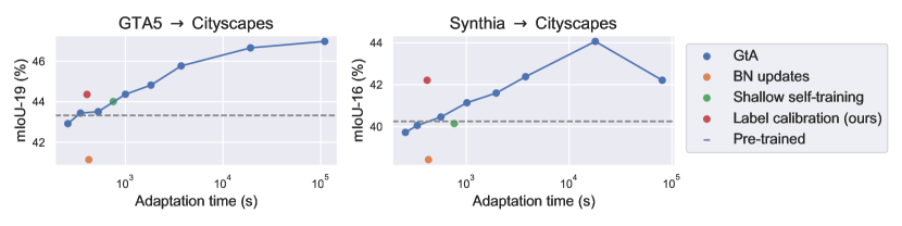
Figure 2: Comparison of the performance and adaptation time of the different methods.

To provide further insights into our method we analyse the estimated prototypes. These are analysed in Figure 3 in the Appendix and show that non-trivial soft-label prototypes are learned.

6 Conclusion

We have proposed a simple and efficient method to calibrate semantic segmentation labels under domain shift and obtain improvements in performance. As part of our method we calculate a soft-label prototype for each class under domain shift and make predictions by finding the nearest prototype. The method is orders of magnitude faster than existing back-propagation based unsupervised source-free domain adaptation methods, but it still leads to noticeable performance improvements.

Appendix A Appendix

Table 2: Our approach works also when using an alternative pre-trained model. Mean mIoU (%) and standard deviation across three runs. mIoU is reported across 19 classes for GTA5 $\rightarrow$ Cityscapes, and across 16 and 13 classes for Synthia $\rightarrow$ Cityscapes.

Approach	GTA5 $\rightarrow$ Cityscapes	Synthia $\rightarrow$ Cityscapes
Pre-trained model	33.97 $\pm$ 0.00	28.17 $\pm$ 0.00 / 32.54 $\pm$ 0.00
Label calibration	34.34 $\pm$ 0.01	29.58 $\pm$ 0.01 / 34.10 $\pm$ 0.01

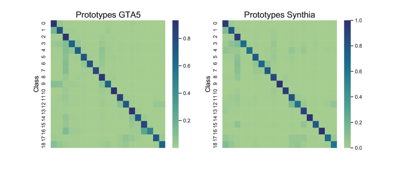
Figure 3: Illustration of the soft-label prototypes for the two different source datasets.

References

- Bojarski et al., (2016) Bojarski, M., Del Testa, D., Dworakowski, D., Firner, B., Flepp, B., Goyal, P., Jackel, L. D., Monfort, M., Muller, U., Zhang, J., Zhang, X., Zhao, J., and Zieba, K. (2016). End to end learning for self-driving cars. In arXiv.
- Chen et al., (2017) Chen, L.-C., Papandreou, G., Kokkinos, I., Murphy, K., and Yuille, A. L. (2017). DeepLab: Semantic image segmentation with deep convolutional nets, atrous convolution, and fully connected CRFs. In TPAMI.
- Chen et al., (2019) Chen, M., Xue, H., and Cai, D. (2019). Domain adaptation for semantic segmentation with maximum squares loss. In ICCV.
- Cordts et al., (2016) Cordts, M., Omran, M., Ramos, S., Rehfeld, T., Enzweiler, M., Benenson, R., Franke, U., Roth, S., and Schiele, B. (2016). The Cityscapes dataset for semantic urban scene understanding. In CVPR.
- Csurka et al., (2022) Csurka, G., Hospedales, T. M., Salzmann, M., and Tommasi, T. (2022). Visual domain adaptation in the deep learning era. In Synthesis Lectures on Computer Vision.
- Ganin et al., (2016) Ganin, Y., Ustinova, E., Ajakan, H., Germain, P., Larochelle, H., Laviolette, F., Marchand, M., Lempitsky, V., Dogan, U., Kloft, M., Orabona, F., and Tommasi, T. (2016). Domain-adversarial training of neural networks. In JMLR.
- Gulrajani and Lopez-Paz, (2020) Gulrajani, I. and Lopez-Paz, D. (2020). In search of lost domain generalization. In arXiv.
- He et al., (2015) He, K., Zhang, X., Ren, S., and Sun, J. (2015). Deep residual learning for image recognition. In CVPR.
- Huang et al., (2021) Huang, J., Guan, D., Xiao, A., and Lu, S. (2021). Model adaptation: historical contrastive learning for unsupervised domain adaptation without source data. In NeurIPS.
- Jackson et al., (2019) Jackson, P. T., Atapour-Abarghouei, A., Bonner, S., Breckon, T., and Obara, B. (2019). Style augmentation: Data augmentation via style randomization. In CVPR workshops.
- Jung et al., (2020) Jung, A. B., Wada, K., Crall, J., Tanaka, S., Graving, J., Reinders, C., Yadav, S., Banerjee, J., Vecsei, G., Kraft, A., Rui, Z., Borovec, J., Vallentin, C., Zhydenko, S., Pfeiffer, K., Cook, B., Fernández, I., De Rainville, F.-M., Weng, C.-H., Ayala-Acevedo, A., Meudec, R., Laporte, M., et al. (2020). imgaug. https://github.com/aleju/imgaug.
- Kouw and Loog, (2021) Kouw, W. M. and Loog, M. (2021). A review of domain adaptation without target labels. In TPAMI.
- Kundu et al., (2021) Kundu, J. N., Kulkarni, A., Singh, A., Jampani, V., and Babu, R. V. (2021). Generalize then adapt: source-free domain adaptive semantic segmentation. In ICCV.
- Kundu et al., (2020) Kundu, J. N., Venkat, N., M, R., and Babu, R. V. (2020). Universal source-free domain adaptation. In CVPR.
- Li et al., (2020) Li, R., Jiao, Q., Cao, W., Wong, H.-S., and Wu, S. (2020). Model adaptation: unsupervised domain adaptation without source data. In CVPR.
- Liang et al., (2020) Liang, J., Hu, D., and Feng, J. (2020). Do we really need to access the source data? Source hypothesis transfer for unsupervised domain adaptation. In ICML.
- Michaelis et al., (2019) Michaelis, C., Mitzkus, B., Geirhos, R., Rusak, E., Bringmann, O., Ecker, A. S., Bethge, M., and Brendel, W. (2019). Benchmarking robustness in object detection: Autonomous driving when winter is coming. In arXiv.
- Richter et al., (2016) Richter, S. R., Vineet, V., Roth, S., and Koltun, V. (2016). Playing for data: Ground truth from computer games. In ECCV.
- Ros et al., (2016) Ros, G., Sellart, L., Materzynska, J., Vazquez, D., and Lopez, A. M. (2016). The SYNTHIA dataset: A large collection of synthetic images for semantic segmentation of urban scenes. In CVPR.
- Saito et al., (2018) Saito, K., Watanabe, K., Ushiku, Y., and Harada, T. (2018). Maximum classifier discrepancy for unsupervised domain adaptation. In CVPR.
- Schneider et al., (2020) Schneider, S., Rusak, E., Eck, L., Bringmann, O., Brendel, W., and Bethge, M. (2020). Improving robustness against common corruptions by covariate shift adaptation. In NeurIPS.
- Sun and Saenko, (2016) Sun, B. and Saenko, K. (2016). Deep CORAL: Correlation alignment for deep domain adaptation. In ECCV.
- Zhang et al., (2021) Zhang, M., Marklund, H., Dhawan, N., Gupta, A., Levine, S., and Finn, C. (2021). Adaptive risk minimization: learning to adapt to domain shift. In NeurIPS.