PhyFu: Fuzzing Modern Physics Simulation Engines

Abstract

A physical simulation engine (PSE) is a software system that simulates physical environments and objects. Modern PSEs feature both forward and backward simulations, where the forward phase predicts the behavior of a simulated system, and the backward phase provides gradients (guidance) for learning-based control tasks, such as a robot arm learning to fetch items. This way, modern PSEs show promising support for learning-based control methods. To date, PSEs have been largely used in various high-profitable, commercial applications, such as games, movies, virtual reality (VR), and robotics. Despite the prosperous development and usage of PSEs by academia and industrial manufacturers such as Google and NVIDIA, PSEs may produce incorrect simulations, which may lead to negative results, from poor user experience in entertainment to accidents in robotics-involved manufacturing and surgical operations.

This paper introduces PhyFu, a fuzzing framework designed specifically for PSEs to uncover errors in both forward and backward simulation phases. PhyFu mutates initial states and asserts if the PSE under test behaves consistently with respect to basic Physics Laws (PLs). We further use feedback-driven test input scheduling to guide and accelerate the search for errors. Our study of four PSEs covers mainstream industrial vendors (Google and NVIDIA) as well as academic products. We successfully uncover over 5K error-triggering inputs that generate incorrect simulation results spanning across the whole software stack of PSEs.

I Introduction

Physics simulation engines (PSEs) are computer software that simulate behavior of physical systems, such as rigid body dynamics (e.g., a steel robot arm), soft body dynamics (e.g., elastic objects), and fluid dynamics (e.g., water simulation). The past few decades have witnessed a boom in using PSEs in production environments, including computer graphics, gaming, virtual reality (VR), and various robotic tasks like robot control, robot parameter design, and trajectory optimization.

Physics simulation techniques have been studied for decades, with numerous high-quality simulation engines developed and commercialized [1, 2, 3, 4, 5, 6, 7, 8, 9]. Notably, conventional PSEs primarily aim for forward simulation, which progressively computes the behavior of the simulated physical system starting from an initial state. In contrast, modern PSEs, often referred to as “differentiable physical simulation engines,” compose both forward and backward simulation phases. While the forward phase still predicts how the simulated system evolves, the defining characteristic of modern PSEs is to offer analytical gradients via a backward phase. The ability of computing analytical gradients makes it possible to perform end-to-end optimization on agent control, and can speedup the optimization process by dozens to hundreds of times [10]. Also, the simulated environments become differentiable, making them technically compatible with training machine learning-based control agents. With the offered gradients, modern PSEs have been demonstrated to accelerate robotics control optimizations by one to four orders of magnitude compared to conventional PSEs [10]. The market for PSEs is also on a rapid rise, with both industrial and academic efforts in developing and enhancing PSEs [11, 12, 13, 14, 15, 16, 17]. The total market share of developing and using PSEs has reached over 10 billion dollars and is expected to grow by over a 10% annually [18, 19, 20]. In addition, PSEs can be highly expensive, with certain surgical PSEs licenses costing over over 10K USD [21].

Nevertheless, production PSEs often comprise dozens to hundreds of thousands of lines of code [22, 14, 23, 13], covering a deep software stack, including the simulation algorithms [15, 17], hardware acceleration modules [22, 23, 16], even sometimes with domain specific language (DSL) that has high expressiveness and efficiency on the simulation primitives, as well as accompanying DSL compilers [22, 23]. Also, the simulated physical effects considered by simulators are complicated, including collision detection, friction, soft body dynamics, and fluid dynamics. Plus, the derivation of gradients in the backward simulation is also challenging, some requiring manual implementation of gradient computation [12], others requiring compilers to generate code for gradient computation directly from the forward simulation code [24, 23]. All of these aspects make PSEs highly complex systems demanding careful design consideration of the PSE vendors. Notably, since PSEs have been applied in various scenarios, from the entertainment industry to safety-critical sectors like surgery robotics [25, 26, 27], bugs in PSEs, in turn, can potentially lead to poor user experience or even catastrophic accidents.

This work presents PhyFu, the first automated, systematic fuzz testing framework for modern PSEs. PhyFu tackles black-box scenarios, allowing testing of (commercial) off-the-shelf PSEs and holistically uncovering bugs in the full software stack of PSEs. Instead of capturing obvious “crash” behaviors (which are rare in PSEs), PhyFu uncovers incorrect simulation outputs (logic bugs) residing in both forward and backward simulation phases of PSEs. To this end, PhyFu generates and mutates the initial states of the system under simulation, and it relies on a principled, clear testing oracle on the basis of Physics Laws (PLs) to uncover incorrect simulations.

Moreover, although arbitrarily generating testing inputs can find a reasonable number of errors during testing, such method struggles to generate inputs towards regions that are difficult to reach, thus omitting some hidden bugs or repeatedly exploring regions that are unlikely to trigger bugs. PhyFu, instead, employs testing feedback to schedule the inputs and to drive the fuzzing exploration toward space with a higher probability of violating our oracle. Besides, the generated states must satisfy the real-world physical constraints to ensure the validity of our testing inputs. It is seen that randomly generating seed inputs can easily break the physical constraints, e.g., a robot arm penetrating the rigid ground. Instead of directly checking the validity of testing inputs (a generally hard process), we generate testing seeds by mutating an initially valid seed while ensuring the validity of our mutations on the fly.

We implement PhyFu targeting four state-of-the-art PSEs. Brax [16], Warp [23], and Taichi [10] are developed by leading industrial PSEs vendors: Google, NVIDIA, and Taichi Graphics, respectively. We also evaluate Nimble [14], an advanced, open-source PSEs developed by Stanford. Our experiments cover 8 combinations of PSEs and physical scenarios, including simulation on balls, robot arms, and soft bodies. PhyFu generates 10K test inputs on each tested setting, and during approximately 20 days of testing, we detected 5,932 inputs that resulted in erroneously simulated results. While the discovered error-triggering inputs do not directly crash PSEs, they silently lead to incorrect simulations. We also found over 20 inputs that triggered crashes, indicating severe security issues like buffer overflow. Through manual analysis and feedback from the PSEs developers, we found that our discovered errors are due to a wide spectrum of reasons spanning the whole stack of PSE software. By the time of writing, two bugs have been promptly fixed. In sum, we make the following contributions:

• We target a crucial yet under-explored need to test PSEs. We, for the first time, propose an automated, systematic fuzzing framework for PSEs in black-box settings.

• PhyFu makes several novel and practical design considerations and optimizations to boost the fuzzing process and uncover more bugs. Also, PhyFu incorporates a set of strategies to ensure the validity of testing inputs.

• Our large-scale evaluation of four modern PSEs subsumes different practical scenarios. Under all conditions, PhyFu detects a substantial number of errors. Further root-cause analysis reveals a diverse set of hidden bugs distributed across the full software stack of PSEs.

We release and will maintain the codebase of PhyFu at [28] to boost future research.

II Preliminary

This section introduces the preliminaries of PSEs. For illustrative purposes, we use a warehouse robotic arm as an example (Fig. 1). Fig. 1a depicts the physical system in which a robot arm releases a ball at initial speed $v_{0}$ downwards. The ball would perform free-fall due to the gravitational force after the release. A sensor is located $L$ meters below the ball’s release point. The sensor would emit a probing signal $T$ seconds after the ball is released from the robot arm. The robot aims to optimize the release speed of the ball so the sensor can sense the ball. In other words, the learning goal of the robot is to control $v_{0}$ to let the ball travel $L$ meters in $T$ seconds.

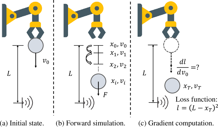
Figure 1: An example of the simulation process of modern PSEs.

Modern PSEs comprise two phases: forward simulation and backward simulation. The forward simulation runs forward and predicts the system’s behavior, while the backward phase outputs analytical gradients that will be helpful for agent learning and control. The details of the backward phase are more intricate, and we introduce the forward simulation first.

Forward Simulation. The forward simulation models the position and velocity of the objects in the physical system as a function of time $t$. The concatenation of position $x$ and velocity $v$ are refered to as state. PSEs allow users to specify the external force, denoted as $\tau$, that is applied on the objects. The external force would determine the change of states as a function of time.

Given the initial state $s_{0}$ at $t=0$ and the external force $\tau$ applied on the objects in the system, the forward simulation phase predicts the state $s(t)$ of the simulated system $\mathcal{S}$ as a function of time $t$ :

$$s(t)=Sim(\mathcal{S},s_{0},\tau,t)$$ (1)

Obtaining $s(t)$ generally requires solving differential equations deduced from physics laws, e.g., Newton’s Second Law.

Example 1.

In the physical scenario of Fig. 1, the state of systems can be described by the dynamics equations in Eq. 2 and Eq. 3:

$$F=mg=m\frac{dv}{dt}$$ (2)

$$\frac{dx}{dt}=v$$ (3)

, where Eq. 2 denotes that the ball would accelerate due to gravity, according to Newton’s Second Law, and Eq. 3 comes from the fact that the time-derivative of position is velocity.

To obtain the function $s(t)$, PSEs would discretize the time $t$ into dozens to hundreds of small intervals, each with length $\Delta t$. Later, as illustrated in Fig. 1b, PSEs deduce the system state $s_{i+1}$ at the time interval $[i\Delta t,(i+1)\Delta t)$ based on the previous state $s_{i}$. The derivation of $s_{i+1}$ from $s_{i}$ is determined by a time-stepping function $TS$:

$$s_{i+1}=TS(s_{i},\tau_{i})$$ (4)

, where $\tau_{i}$ is the external force applied on the objects at the given time interval. $TS$ is determined by the differential equations to be solved.

Backward Simulation. Learning and control tasks, e.g., a robot controlling the initial velocity to shoot a basketball into the basket, typically aim at deciding an initial state $s_{0}$ that would lead to the optimal objective function $h(s_{t})$ defined on the final state $s_{t}$. In general, the key requirement of the agent learning process is to enable access to the analytical gradients, $\partial h(s_{T})/s_{0}$, of function $h$ w.r.t. the initial state $s_{0}$, as this would enable an end-to-end optimization on the objective function directly. It has been shown that analytical gradients can speed up the optimization process by tens to hundreds of times [24, 16].

As one key feature, modern PSEs offer the ability to compute analytical gradients in the backward simulation phase. This way, PSEs provide feedback to guide learning-based agents, like robotics control models, to gradually improve their performance using gradients and reach a user-specified objective. In contrast to the forward simulation, gradient computation runs backward, starting from a loss function defined on the final state and propagating the gradients to the initial state.

Consider Fig. 1c, suppose the forward simulation process determines that the ball would be located at $x_{T}$ after $T$ seconds, where $x_{T}\neq L$. Given an objective such that the ball is required to be at location $L$ at time $T$ when a probing signal is emitted, the robot arm learns to gradually adjust the initial speed, $v_{0}$, of the ball. The optimization goal can be formulated as Eq. 5:

$$\operatorname*{arg\,min}_{v_{0}}\left|x_{T}-L\right|^{2}$$ (5)

Modern PSEs facilitate solving Eq. 5 in a principled manner by providing the gradients of the simulation process and making the entire process differentiable. Thus, the simulation process can be smoothly integrated into training a learning-based agent. Fig. 1c illustrates how PSEs can be employed. Given the loss function defined as $l=(L-x_{T})^{2}$, the backpropagation first computes $dl/dx_{T}$, which can be easily computed by automatic differentiation frameworks such as PyTorch [29]. Then, PSEs can derive the analytical gradients $dx_{T}/dv_{0}$ (see below for details). The $dl/dx_{T}$ and $dx_{T}/dv_{0}$ can then be combined via chain rule, resulting in the end-to-end gradient $dl/dv_{0}$, i.e., the gradient of the loss value $l$ w.r.t. the parameter $v_{0}$. Having obtained the end-to-end gradients, parameters in a learning-based agent like robot arm can be consequently optimized using methods like gradient descent.

Various methods have been proposed for gradient derivation. Some engines formulates the simulation process as a linear complementarity problem (LCP) [14, 12] and derive gradients accordingly, and some treat the simulation as a non-linear complementarity problem (NCP) [17, 11] that conforms to the physical laws better but is more costly to solve. Some engines also use compliant models [16, 30], convex optimization models [31], and position-based dynamics [23].

III Overview of PhyFu

We aim to uncover logic bugs in PSEs. As in Section II, PSEs feature both forward and backward phases to train learning-based complex agents [10]. The forward phase computes the final state $s_{T}$ of a physical system at time $T$ for a given initial state $s_{0}$. The backward, gradient-computation phase starts from a loss function defined on the final state, and propagates the gradients backwards to the initial state.

To systematically subsume both forward and backward phases, we propose a testing oracle based on principled Physics Laws (PLs). Before introducing the PLs used, we first list some assumptions below:

Assumptions and Application Scope. We assume a set of reasonable pre-conditions so that the PLs we use can hold. The assumptions and their corresponding proofs are already well-researched in a category of mathematics and physics problem called the “Inverse Problem” [32, 33], which deals with whether the initial state $s_{0}$ for an observed system’s final state $s_{T}$ is unique and proposes strategies to find such $s_{0}$. Due to the complexity of the strict definitions and proofs, we can only briefly list the high-level ideas of the full assumption set in a less sound and complete form, so as to facilitate the understanding of audience from general background:

1. The physical process is deterministic and non-chaotic.

2. The final state after the forward physical process has to depend continuously on the initial state.

3. No friction is allowed in the physical system.

We note that the above assumptions can reasonably hold in real-world physical systems and PSEs. The first two assumptions are easily satisfied in common use cases of PSEs, such as robotic and soft-body simulations. The third assumption is a common setting in real-world usage of PSEs, since typical physical scenarios under simulation, such as rigid simulation [24], molecular simulation [34, 35] and fluid simulation [36, 37], generally configure the friction force to be zero, as the support for friction from PSEs is not mature enough and still an open-research problem [11, 24, 15].

We present the following important fact, denoting the uniqueness of $s_{0}$ (on the condition of assumptions listed above):

Forward Testing Oracle. Based on the property of uniqueness for $s_{0}$ in the theory above, we formulate our testing oracle to test the forward simulation process as:

Definition 1 (Forward Testing Oracle).

Let $f(s_{0})=s_{T}$, where $f$ is the forward simulation mapping initial state $s_{0}$ to final state $s_{T}$. For $\forall s_{0}^{\prime}$ s.t. $f(s_{0}^{\prime})=s_{T}$, we assert if $s_{0}^{\prime}=s_{0}$.

Oracle in Definition 1 asserts that the final state should not be identical whenever two initial states are distinct. If this property is not adhered to, it indicates the presence of bugs in the forward simulation phase of the tested PSEs.

Backward Testing Oracle. To test the analytical gradients yielded from the backward simulation, we use a theoretic property of gradients:

Theorem 1 (Theory of Gradient-Based Optimization).

Consider a differentiable multi-variate function $h(x)$ and its global minimal point $x^{*}$. Starting from a point $x=x^{*}+\Delta x^{0}$ that lies sufficiently close to $x^{*}$, perform gradient descend about $\Delta x$ until convergence:

$$\Delta x^{k+1} =\Delta x^{k}-\alpha^{k}g(\Delta x^{k})$$ (6)

, where $k$ is the iteration number, and $\alpha^{k}$ is the update step length. Then $h(x)$ is bound to converge globally to $h(x^{*})$ [42].

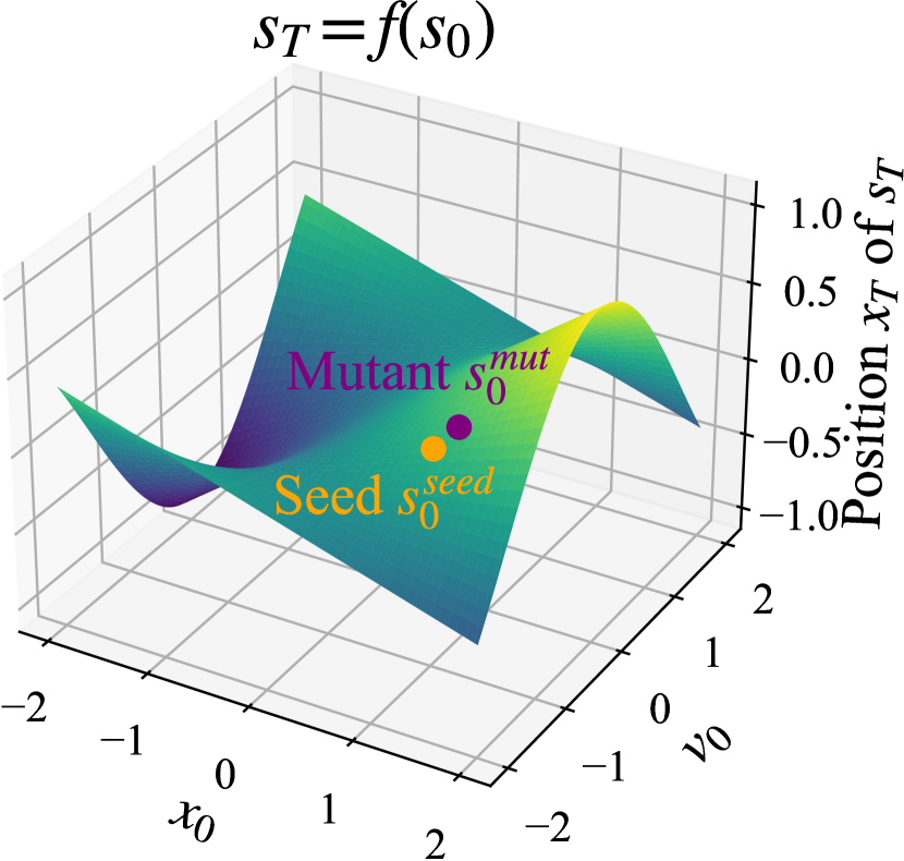
(a) Seed and mutant.

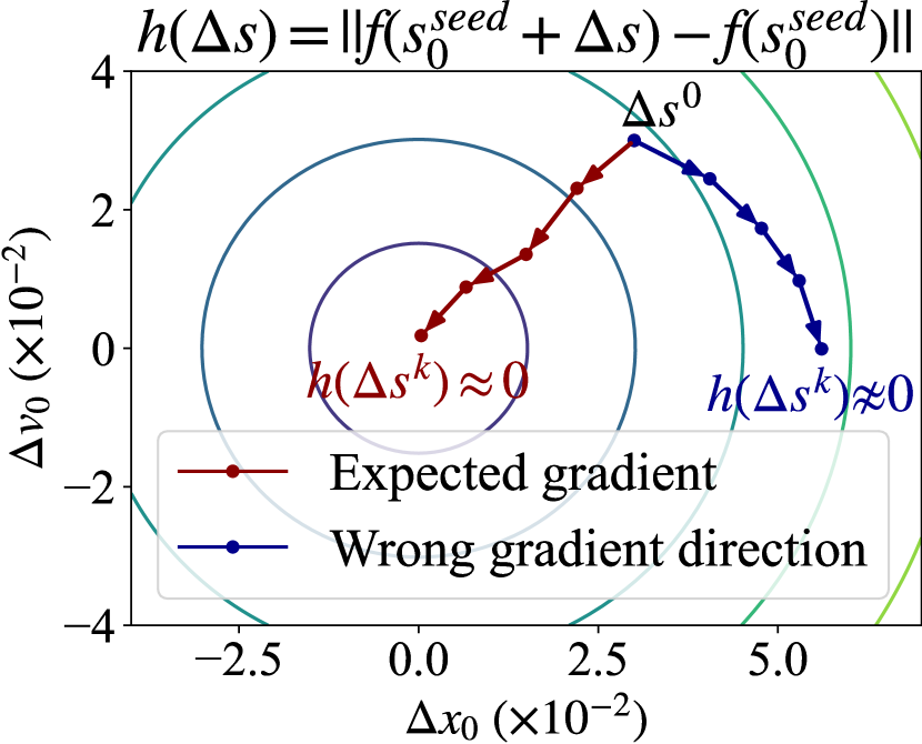
(b) Optimize $\Delta s$ with gradients.

Figure 2: Illustration of the backward oracle. In (a), $s_{0}^{mut}$ is obtained by adding a small $\Delta s$ with $s_{0}^{seed}$; (b) shows two traces of gradient descent iterations starting from the initial $\Delta s$, where red and blue traces are guided by the correct and wrong gradients, respectively. The intuition of our backward oracle is reflected from the blue trace.

We illustrate the ideas of our backward simulation testing approach in Fig. 2. Denote the forward simulation function as $f$, which maps an initial system state $s_{0}$ to the final state $s_{T}$. In Fig. 2(a), the position $x_{0}$ and velocity $v_{0}$ component of initial state $s_{0}$ are shown on the x-y plane, and the z-axis shows the position component $x_{T}$ of the corresponding final state $s_{T}$ ($s_{T}=f(s_{0})$). Given an initial state $s_{0}^{seed}$ and its final state $s_{T}^{seed}$, we randomly add a small perturbation, $\Delta s$, to $s_{0}^{seed}$, and obtain a mutated initial state $s_{0}^{mut}$. We then aim to find the minimum of the objective function:

$$h(\Delta s)=\lVert f(s_{0}^{seed}+\Delta s)-f(s_{0}^{seed})\rVert$$ (7)

, by executing the gradient-descend algorithm on $\Delta s$ under the guidance of gradients $g(\Delta s)$ computed from the backward simulation. Fig. 2(b) shows two example optimization traces, both of which start from the initial $\Delta s^{0}$ and end in their respective $\Delta s^{k}$ after $k$ gradient-descend iterations. The red trace shows the optimization trace guided under the correct gradients, while the blue one is guided by buggy gradients. After $k$ iterations, the red one successfully finds the minimal point, i.e., when $h(\Delta s)\approx 0$, while the blue one causes $h(\Delta s)$ to deviate from its minimum further and further away due to the wrong direction of computed gradients. Based on Theorem 1, we assert the following oracle to test backward simulation:

Definition 2 (Backward Testing Oracle).

Starting the gradient descend on a small initial $\Delta s$, the objective function $h(\Delta s)$ should converge to 0 after sufficient number of iterations.

The proof of Definition 2 can be readily derived from Theorem 1, and we leave the full proof on our website [28] due to space limit.

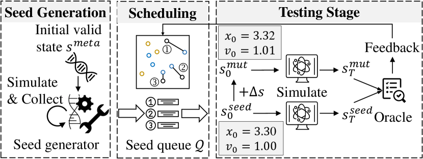
Figure 3: Testing pipeline.

IV Design of PhyFu

Design Overview. PhyFu delivers an automated, systematic fuzzing framework to test modern PSEs with respect to our forward and backward testing oracles. Fig. 3 illustrates the pipeline of PhyFu, which consists of three parts: ➀ seed generation, ➁ seed scheduling, and ➂ testing.

➀ Seed Generation. PhyFu generates a pool of states $\mathcal{C}$ as the testing seeds for the fuzzing. A state $s^{seed}$ in the seed pool $\mathcal{C}$ comprises the position and the velocity of objects in the system simulated by the PSE under test. The generated seed states will be scheduled and fed into the testing stage for uncovering erroneous simulations. We propose a set of design choices to ensure the validity of seed states during the seed generation phase (see Section IV-C).

➁ Seed Scheduling. Testing by randomly generating seeds can suffer from inefficiency and ineffectiveness issues. Since the simulation process of PSEs is highly time-consuming (often a testing campaign takes several to dozens of hours; see Table II), to uncover more bugs with a reasonable resource, we employ a scheduling algorithm to prioritize seeds that are more likely to trigger bugs. The seeds generated from the seed generator are enqueued and sorted in a seed queue $\mathcal{Q}$, and are dequeued to be used in the testing stage based on their priority.

➂ Testing. The testing stage dequeues a seed $s^{seed}$ from the seed queue, and uses it as the initial state, $s_{0}^{seed}$, for the simulation. The initial state is added with a sufficiently small mutation, $\Delta s$, to obtain a mutated initial state $s_{0}^{mut}$. We will then check the seed and mutant against our forward and backward oracles, and provide testing outcomes as feedback to the seed scheduling stage to prioritize unused seeds.

IV-A Fuzz Testing

Algorithm 1 Fuzz Testing.

1:function Fuzzing(Corpus of Seed Inputs $\mathcal{C}$, $T,\mathcal{E}$)

2:    $\mathcal{Q}\leftarrow\mathcal{C},\mathcal{O}\leftarrow\varnothing,\mathcal{F}\leftarrow\varnothing$

3:    for 1 … MAX_ITER do

4:        $s_{0}^{seed}\leftarrow$ Dequeue($\mathcal{Q}$)

5:        $\tau\leftarrow randForce()$ $\triangleright$ Randomly apply external forces.

6:        $s_{T}^{seed}\leftarrow$ Forward($\mathcal{E},s_{0}^{seed},\tau,T$)

7:        $\Delta s\leftarrow{\color[rgb]{0,0,1}\textit{{Mutate}}}(s_{0}^{seed}$) $\triangleright$ Generate small perturbation.

8:        for 1 … MAX_GRAD_ITER do

9:           $s_{0}^{mut}\leftarrow s_{0}^{seed}+\Delta s$ $\triangleright$ Add mutation.

10:           $s_{T}^{mut}\leftarrow$ Forward($\mathcal{E},s_{0}^{mut},\tau,T$)

11:           $\mathcal{L}\leftarrow\lVert s_{T}^{seed}-s_{T}^{mut}\rVert^{2}$ $\triangleright$ Compute loss.

12:           if $\mathcal{L}<\epsilon_{B}$ then

13:               break           

14:           $g\leftarrow\textsc{Backward}(\mathcal{E},\mathcal{L})$ $\triangleright$ Backward simulation.

15:           $\Delta s\leftarrow$ Update($\Delta s,g$) $\triangleright$ Gradient descend.         

16:        if  ViolateOracle($s_{0}^{seed},s_{0}^{mut},s_{T}^{seed},s_{T}^{mut},\mathcal{L}$)  then

17:           Add($\mathcal{O},s_{0}^{seed}$) $\triangleright$ Include in the buggy set.         

18:        Add($\mathcal{F},s_{0}^{seed}$) $\triangleright$ Mark as already-fuzzed.

19:        Schedule($\mathcal{Q},\mathcal{O},\mathcal{F}$) $\triangleright$ Seed scheduling.     

20:    return Buggy states $\mathcal{O}$

Algorithm 1 formalizes the fuzzing procedure, which tests a target PSE $\mathcal{E}$ and yields a set of error-triggering inputs $\mathcal{O}$ that violates our testing oracles, either Definition 1 or Definition 2. The core components of Algorithm 1 can be summarized below:

• Mutate takes the initial seed state $s_{0}^{seed}$ as input and generates a small perturbation $\Delta s$, which will later be added to $s_{0}^{seed}$ to obtain a mutated initial state $s_{0}^{mut}$. The mutant $s_{0}^{mut}$ will be used to initiate the fuzzing campaign.

• Update optimizes the amount of perturbation, $\Delta s$, based on its gradients $g$ computed by the backward simulation. The function applies a step of the gradient-descend algorithm, as the one mentioned previously in Eq. 6.

• ViolateOracle checks whether our oracle, Definition 1 or Definition 2, is violated. It takes as input the initial and final states of both the seed and the mutant, as well as the final loss value after the gradient descend, and checks against the forward and backward oracles.

• Schedule arranges the order of the seeds. The fuzzing seeds are stored and sorted in a queue $\mathcal{Q}$, and are dequeued based on their priority. To maximize the efficiency of fuzzing and find more bugs in a limited time budget, we leverage a feedback-driven scheduling algorithm to prioritize the seeds (see Section IV-B).

Our fuzzing algorithm comprises a series of carefully designed steps to trigger simulation failures of the target PSE. Overall, Algorithm 1 contains the following steps:

Initialization. As the entry point of our procedure, Fuzzing takes as input a corpus of seed inputs $\mathcal{C}$, a simulation time span $T$, and a target PSE $\mathcal{E}$. $\mathcal{C}$ is used to initialize a queue $\mathcal{Q}$ (line 2), which determines the order of seeds during fuzzing.

Fuzzing Loop. In each iteration, we pop out the seed with the highest priority (see below for Schedule), and use it as the seed initial state $s_{0}^{seed}$ (line 4), whose corresponding final state $s_{T}^{seed}$ is obtained from the forward simulation of $\mathcal{E}$ (line 6). Based on $s_{0}^{seed}$, we generate a small perturbation amount $\Delta s$ (line 7), which will later be added over the seed initial state $s_{0}^{seed}$ to obtain a mutated initial state $s_{0}^{mut}$ (line 9).

Gradient Descend Iterations. The gradient desend iterations (lines 8–15) follow the steps introduced in Section III to check the backward simulation. Starting from the initial perturbation amount $\Delta s$ generated in line 7, the variable $\Delta s$ is iteratively updated under the guidance of its gradients, $g$, from the backward simulation. The iteration loop is terminated if the loss value $\mathcal{L}$, which is defined as the distance between the final states $s_{T}^{seed}$ and $s_{T}^{mut}$, is small enough (line 12), or the number of iterations reaches a pre-defined threshold $MAX\_GRAD\_ITER$ (line 8).

Oracle Violation Checking. After the gradient descend iterations, ViolateOracle detects any violation against the forward or backward oracle.

Backward Oracle Checking. The backward oracle checking examines the loss value $\mathcal{L}$, which is iteratively updated under the guidance of gradients $g$. If $\mathcal{L}>\epsilon_{B}$, then the backward oracle, Definition 2, is deemed to be violated, and gradients from the backward simulation phase are considered buggy.

Forward Oracle Checking. Following Definition 1, when the final states of seed and mutant are close to each other, we check if their corresponding initial states are close to each other. Specifically, ViolateOracle would report oracle violation if $\lVert s_{T}^{seed}-s_{T}^{mut}\rVert<\epsilon_{F}$ (near-identical final state) while $\lVert s_{0}^{seed}-s_{0}^{mut}\rVert>\epsilon_{I}$ (distinct initial state).

Adaptive Fuzzing Scheduling. After each fuzzing iteration, $s_{0}^{seed}$ would be included in the output set $\mathcal{O}$ if an oracle violation is detected (line 17). The buggy set $\mathcal{O}$, together with the set $\mathcal{F}$ of all the already-used seeds, will be used as feedback to prioritize the seeds in the seed queue $\mathcal{Q}$ (line 19). Details of prioritization are introduced in Section IV-B.

IV-B Feedback-Driven Seed Prioritization

Inefficiency of Random Seed Selection. The testing campaign is seen to be slow in evaluations (see Table II). The forward simulation process requires discretizing the simulation time span $T$ into dozens to hundreds of small steps (see Section II), and iteratively applying a non-trivial time-stepping function Eq. 4 for each small step; the backward simulation also consumes comparable time as the forward simulation. As such, the testing process can take hours or dozens of hours to finish, spending a considerable amount of time on the simulation process itself. Randomly selecting a seed from the seed pool can be inefficient, as it can waste time executing the costly simulation on seeds that are not likely to trigger errors.

Prioritization Strategy. To uncover more errors in a limited time budget, we employ the Adaptive Random Test (ART) algorithm [43] to prioritize seeds with higher probabilities to trigger errors. The intuition behind ART is that neighbors of a non-failure-inducing seed are also less likely to cause errors, while neighbors of a failure seed are also more likely to cause failures. Algorithm 2 shows the workflow of ART. Given the set of error-triggering seeds $\mathcal{O}$ and the set of already-used seeds $\mathcal{F}$, ART would first derive non-failure-causing set $\mathcal{U}$ by taking the difference of $\mathcal{F}$ and $\mathcal{O}$ (line 2). For each seed to schedule in the seed queue (line 4), it will compute the minimal distance to all the non-failure-causing seeds (lines 5–7), and take the computed minimal distance as the corresponding energy value (line 8). The seeds in $\mathcal{Q}$ will be sorted in descending order according to their energy value (line 9). ART allows us to focus our testing efforts on the most promising seeds, increasing the chances of finding bugs and wasting less time exploring uninteresting states; see Section VI-C for empirical results.

Algorithm 2 Feedback-Driven Test Case Prioritization

1:function Schedule(Seed queue $\mathcal{Q}$, Buggy set $\mathcal{O}$, Full set $\mathcal{F}$)

2:    $\mathcal{U}\leftarrow\mathcal{F}-\mathcal{O}$ $\triangleright$ $\mathcal{U}$ as seeds that don’t trigger errors.

3:    $EnergyList\leftarrow zeros(\mathcal{Q}.size)$

4:    for $i$ in range($\mathcal{Q}.size$) do

5:        $minDist\leftarrow+\infty$

6:        for $u$ in $\mathcal{U}$ do $\triangleright$ Find minimal distance to seed states in $\mathcal{U}$.

7:           $minDist\leftarrow min(minDist,\lVert u-\mathcal{Q}[i]\rVert)$         

8:        $EnergyList[i]\leftarrow minDist$     

9:    Sort($\mathcal{Q}$, $EnergyList$) $\triangleright$ Sort in descending order.

IV-C Seed Validity Ensurance

It is critical to ensure that our testing seeds, denoting initial states $s_{0}^{seed}$ of the tested PSE, are valid in the physical world. Otherwise, “bugs” found by the testing process may be less interesting or even false positives. Typically, the requirements for the seed validity can be encoded as state constraints, or referred to as constraints. Constraints vary from scenario to scenario. We will use the example of two balls colliding with each other to illustrate the concept of constraints:

Example 2.

In a simulation involving only rigid objects, the states of two balls must satisfy a set of constraints, namely, “intersection constraint”. A rigid object cannot penetrate another rigid one. In the situation of two balls, the constraints are expressed as:

$$\sqrt{(x_{1}-x_{2})^{2}+(y_{1}-y_{2})^{2}+(z_{1}-z_{2})^{2}}\geq 2r$$ (8)

, where $r$ is the radius of the two balls, and $x_{i},y_{i},z_{i},i\in\{1,2\}$ are the 3D coordinates of ball $i$.

Two Sources of Invalid Seeds. Performing simulations over a physically infeasible initial state, e.g., a ball penetrating another ball, would also likely lead to an invalid final state. We clarify two sources of invalid seed initial states: ➀ seed generation without respecting the constraints; ➁ internal bugs in PSEs. Oracle violations due to ➀ should be deemed as false positives (FPs). In contrast, wrong simulation results due to ➁ are true positives (TPs), since the invalid seeds are due to bugs in the tested PSEs. We should avoid invalidity issues from ➀.

Invalidity of Random Seed.  Our preliminary experiments show that randomly generating seed states could easily lead to invalid states from source ➀. For instance, when arbitrarily generating the initial rotational angle of a robot arm, we find that a large portion (over 70%) of the generated states lead to apparently invalid states, such as the palm penetrating a hard surface. Even worse, typical PSEs often lack a comprehensive ability to detect and reject simulation requests for invalid initial states. For example, in the Brax Physics Engine [16] (a Google product), even though the palm of a UR5E robot arm is obviously under the surface of the ground, the simulation engine does not detect and warn the user about the issue of such invalid state, but continues simulation as usual. However, the invalid seeds are not due to internal bugs of PSEs, but arise from wrongly designed seed generation scheme.

Naive Method: Generate-then-Check (GTC).  A potential approach to ensuring state validity is randomly generating a seed state and rejecting invalid ones. However, we emphasize that such a generate-then-check (GTC) approach could not easily work. The constraints are varied across different physical environments. Hence, it is challenging to present a unified solution for state validity checking. Moreover, the format of constraint equations inside a single physical scenario may be complex, sometimes not even explicitly representable [44, 45].

Our Solution: Simulate-then-Collect (STC). In contrast to GTC, which checks the validity of a generated seed state and rejects invalid, we propose a simulate-then-collect (STC) approach. The high-level idea of STC is to start from an initially valid state $s_{meta}$ (also called meta seed, typically can be chosen to be the default initial state shipped by the PSE under test) whose validity can be guaranteed through manual efforts, and run forward simulation to collect a trace $tr=s_{meta},s_{1},s_{2},\ldots,s_{n}$. The states on the simulation trace $tr$ would then be collected and added to the seed pool $\mathcal{C}$ as the fuzzing seeds. To enhance the diversity of generated seeds, the external forces $\tau_{i}$ during the transition from state $s_{i-1}$ to $s_{i}$ are varied across different $i,i\in[1,n]$.

Formally, to see why the STC approach would generate valid states, we present the following theorem:

Theorem 2 (Theorem of State Validity).

Assuming the time stepping function $TS$ of a PSE is consistent with physics laws, any reachable state $s_{i}$ starting from an initial valid state $s_{meta}$ should also be valid.

Theorem 2 can be easily proved by math induction (details are on [28]). We admit that when the time stepping function $TS$ is buggy, the collected seed states could be invalid in the first place. However, this should not be a concern, as to our observation, invalid seeds lead to incorrect simulation results (true positive bugs), which will be detected by PhyFu later.

V Implementation

PhyFu is implemented in about 4K LOC [28]. The key hurdle of our implementation is accommodating the large differences between evaluated PSEs (see Section VI-A). Each PSE uses a different domain-specific language (DSL) to describe its simulated environment and perform forward simulation and gradient computation. The algorithms under each PSE are also distinct from each other. Still, our testing method is agnostic to the underlying details of the tested PSEs. Moreover, we spent non-trivial efforts to refactor our code so that extending our testing method to a different testing configuration requires little engineering effort. See our codebase and documentation (including instruction on extension) at [28].

VI Evaluation

In this section, we aim to answer the following research questions (RQs): RQ1: Can PhyFu effectively uncover errors in the modern PSEs? RQ2: To what extent can the seed scheduling algorithm facilitate the fuzzing campaign? How much overhead does the scheduling process incur? RQ3: What are the characteristics of errors uncovered by PhyFu? RQ4: What root causes lead to the failures of the tested PSEs? We answer the four RQs from four aspects, respectively:

1. We evaluate our testing methods on eight configurations in total, including four popular PSEs and two physical scenarios per PSE. We show that our testing campaign can fruitfully uncover error-triggering inputs on each setting.

2. We use ablation study to show that our scheduling algorithm introduced in Section IV-B can significantly boost error-discovery efficiency while incurring negligible overhead.

3. We categorize all of our discovered error-triggering inputs to facilitate understanding our findings.

4. We launch root cause analysis towards our findings through manual analysis and developer feedback. We further give a representative example for each of our tested PSEs on the bug root cause.

VI-A Experiment Setting

Evaluated PSEs. Developing PSEs with both forward and backward simulation capabilities has been a hot topic in recent years, and numerous PSEs [13, 15, 17, 12, 11] emerged in just a short period; covering so many existing PSEs can be impractical. We carefully review existing PSEs and choose our testing targets based on their quality, usability, and popularity. We also consider the diversity of testing targets, covering PSEs from both academy and industry. Ultimately, we select four PSEs as our evaluation targets, namely, Taichi Graphics [24], Nimble [14], Warp [23], and Brax [16]. Nimble is a popular PSE developed by Stanford, while Warp and Brax are NVIDIA and Google’s products, respectively. Taichi Graphics originates from MIT researchers and later transforms into a 50M-startup company, with over 22.4K stars [22] on GitHub.

Physical Simulation Scenarios. We choose two categories of scenarios to evaluate our tested PSEs: one that is fundamental in physical simulation and generally supported by existing PSEs, and the other that is specific to each of our tested PSEs. For the first category, we choose the simulation of the behavior of a group of balls bouncing between walls, as the simulation of balls under collision is a base stone for building up complex simulation cases, such as molecular simulation [34, 35, 37] and fluid simulation [36, 46, 47]. Also, as a fundamental simulation scenario, ball collision is widely supported by existing PSEs [48, 49]. As for the second category, we select an engine-specific use case for each PSE (four in total). The details of all the evaluated combinations of PSEs and scenarios can be found in Table I. Our tested PSEs are at their latest versions by the time of writing (except Nimble, see our discussion later). In total, our evaluation consists of eight configurations (four PSEs and two scenarios per PSE). For each configuration, we generate 10K testing inputs and feed the generated testing inputs into PSEs for fuzzing.

TABLE I: Evaluated configurations. “All” means the all the PSEs are evaluated on the scenario of “Balls.”

PSE	PSE Version	Physical Scenario	Brief Description
All	NA	Balls	A group of balls bouncing around walls and colliding with each other.
Brax	0.1.0	UR5E	A UR5 robot arm that can fetch or deliver items in the factories.
Nimble	0.8.32	Catapult	A robot with three joints batting balls.
Warp	0.7.2	Snake	A set of rods chained in sequence that looks like a snake.
Taichi	1.4.1	DiffMPM	An elastic object jumping and moving forward on the ground by deformation.

Hyper-parameter Settings. As mentioned in Section IV-A, we use threshold $\epsilon_{B}$, $\epsilon_{F}$ and $\epsilon_{I}$ to check our testing oracles. We also need to decide the initial perturbation amount of $\Delta s$ on $s_{0}^{seed}$. Deciding proper values for these parameters is quite challenging and requires manual efforts (see our clarification on this in Section VII). To do so, we repeat the process of generating 1K testing inputs under a tentatively-decided parameter value and adjusting the value based on manual inspection on possible false positives (FPs) of findings. We release all parameter settings in the codebase [28] to enable reproducing results and research transparency.

VI-B RQ1: Overall Effectiveness

This section studies RQ1, i.e., the effectiveness of our methods on bug discovery. To that end, we show the total execution time and the number of errors we find on each combination of tested PSEs and physical scenarios. Table II reports the statistics of our experiment. The eight testing settings are abbreviated via the first letter of the tested PSE and the physical scenario, e.g., “TD” denotes “Taichi DiffMPM”.

Processing Time. We execute all experiments on a Ubuntu 18.04 server with an NVIDIA RTX 2080 Ti GPU ported with CUDA 12.1, an Intel(R) Xeon(R) E5-2683 CPU, and 256GB RAM. The third row, “Time (hr)”, in Table II reports the execution time (in terms of the number of hours) of each configuration. Overall, the physical simulations on PSEs are slow and take dozens to hundreds of hours to finish, as the simulation process requires applying the time-stepping function (i.e., Eq. 4) for dozens to hundreds of steps. DiffMPM (TD) is the most time-consuming one since its simulation requires discretizing the space into thousands of small grids. The computation of Balls is lightweight and only takes several hours to finish. An exception is Brax/Balls (BB), possibly due to its language constraints of disallowing in-place modifications of array elements [50] and thus wasting time on allocating new arrays for each modification operation.

Discovered Errors. We generate 10K testing inputs for each tested combination of PSEs and physical scenarios. The second row, “#Errors”, in Table II lists the number of erroneous inputs discovered in each tested setting. Although all of our tested PSEs are developed by industry giants or highly experienced researchers from academia, we can still reveal a considerable number of errors. In total, we find 5,932 testing inputs that can trigger misbehaviors in the simulation outputs. Specifically, the “Balls” scenarios on Brax and Taichi physics engines have the highest number of erroneous testing inputs (over a thousand). Although the physical laws governing the behavior of balls are conceptually simple, the computer simulation of balls is challenging to be implemented flawlessly (see a discussion of the author of Taichi on one of the well-known challenges [10]), and the intricate interactions between balls and walls may manifest the hidden bugs and thus be captured by our testing method. Overall, our method uncovers at least 400 erroneous cases in all testing settings, demonstrating its effectiveness.

Discovered Crashes. Although our testing method primarily focuses on logic bugs, i.e., bugs that produce incorrect results, we also find several crashes that cause severe consequences like segmentation fault during our testing campaign. When a crash happens, we start a new process and continue the generation and execution of testing inputs using a different random number. During the simulation of DiffMPM on Taichi, we find 23 crashes that lead to invalid memory access in GPU. We also encounter a crash in Nimble that constantly produces segmentation fault and stops the testing process altogether. The crash is due to a regression bug in the Nimble physics engine. We thus resort to a relatively older version (0.8.32) of Nimble.

TABLE II: Results overview (10K inputs per testing setting). We leave discussion on “SS (min)” in RQ2.

	BB	BU	NB	NC	TB	TD	WB	WS	Total
#Errors	1183	475	709	833	1128	455	427	732	5932
Time (hr)	28.2	23.4	3.8	5.5	1.5	104.1	1.5	24.0	192
SS (min)	65	43	6	2	2	10	4	5	168

VI-C RQ2: Effectiveness and Overhead of Seed Scheduling

This section aims to answer RQ2, i.e., the effectiveness of the guided seed scheduling algorithm in Algorithm 2, and its incurred time overhead. To answer this question, we perform an ablation study by excluding the seed scheduling algorithm in our testing pipeline.

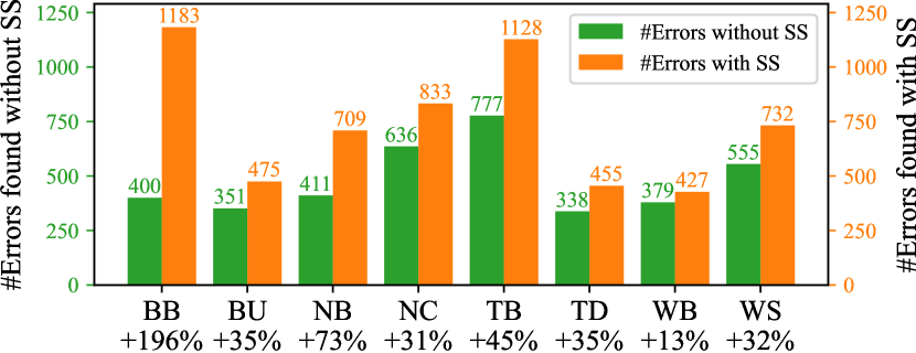
Figure 4: #Errors discovered without and with seed scheduling (SS). The relative increase (%) on #errors of SS is on x-axis.

Ablation Study. We disable the seed scheduling algorithm and launch fuzzing with exactly the same setting as Section VI-B. We also record the time spent executing the seed scheduling algorithm itself. Fig. 4 shows the comparative results between enabling seed scheduling (abbreviated as “SS” in the figure) and disabling it. The green and yellow bars show the number of errors discovered without and with SS, respectively. The meaning of first row of labels on the x-axis is the same as Table II, showing all the eight testing combinations; the second row shows the relative percentage of increase in the number of errors uncovered with SS compared to without SS.

Overall, the seed scheduling method is seen to significantly boost the error-finding ability. The scheduler typically results in a 30 to 40 percent rise in the number of uncovered errors, with the highest increase being 195% and all exceeding 13%. The increase is most visible when testing the scenario of “Balls” on Brax (BB) and Nimble (NB) engines. Through a later manual analysis on the root cause analysis of the error-triggering inputs, we find that the conditions to trigger bugs in those two testing settings are quite intricate. For instance, unveiling some errors requires multiple objects colliding with each other simultaneously. Such strict requirements on the error-triggering condition render the random algorithm struggling in error discovery. In contrast, the seed scheduling algorithm can prioritize seeds that are more likely to satisfy such conditions.

Time Overhead of Seed Scheduling. Despite the effectiveness of our seed scheduling algorithm, we find that it only adds negligible amount of time to the total execution time of fuzzing. The last row, “SS (min)”, of Table II, shows the extra time overhead (in terms of minutes) of seed scheduling (abbreviated as “SS”). In most cases, the time spent on the seed scheduling algorithm is within several minutes. In contrast, the total execution time of the whole fuzzing campaign, as also presented in the row “Time (hr)” in the same table, is typically hours to dozens of hours, far exceeding the time spent on the seed scheduling. The efficiency of the seed scheduling algorithm partly comes from its succinctness; also, the algorithm itself can be implemented in terms of simple vector computation primitives, such as dot products, which existing vector libraries already optimize. An exception is the Brax engine, spending around or more than an hour on the scheduling algorithm. The reason might be similar to its long execution time, as explained in Section VI-B. However, compared to the total amount of time on the simulation (more than 20 hours), the percentage of the overhead (3%) is still low.

VI-D RQ3: Characteristics of the Errors

This section focuses on RQ3. To answer this question, we utilize a set of heuristics to classify our findings and summarize some patterns and the distribution of our discovered errors.

Error Categories. As mentioned in Section III, our testing method asserts both the forward and backward oracles. Furthermore, forward and backward errors may exhibit various patterns. We define the following heuristics to classify the errors on a finer scale:

Position & Velocity Error of System: The forward simulation process essentially deals with computing states (see Eq. 4), which uniquely defines the system’s current situation under simulation. As introduced in Section II, a state comprises the velocity part and position part. We thus characterize the forward errors by whether the position or the velocity is incorrectly computed during the forward simulation.

Direction & Extent Error of Gradient: The backward simulation computes the gradients w.r.t system initial states. A gradient is a vector with direction and extent. Accordingly, we classify backward errors into direction errors and extent errors.

Criteria for Error Classification. When classifying forward errors, we compare the mutated initial state $s_{0}^{mut}$ with its corresponding seed initial state $s_{0}^{seed}$, and deem it to be a position (velocity) error if their position (velocity) components of the state significantly deviate. As for determining whether the gradient direction is wrong for a backward error, we use the following heuristic:

$$\arccos\frac{-g(\Delta s)^{T}\Delta s}{\lVert g(\Delta s)\rVert\lVert\Delta s\rVert}<\theta_{D}$$ (9)

, where $\Delta s=s_{0}^{mut}-s_{0}^{seed}$, $g(\Delta s)$ is the gradients computed by the PSE w.r.t. $\Delta s$, and $\theta_{D}$ is a threshold, which is empirically set to $\pi/2$. Eq. 9 asserts that the gradient vector $g(\Delta s)$ should point to the direction close to $-\Delta s$. A violation of Eq. 9 indicates erroneous gradient direction computed from PSE.

In terms of classifying the gradient extent errors, we use the following heuristic:

$$\forall||h(\Delta s_{1})||>||h(\Delta s_{2})||,||g(\Delta s_{1})||\geq||g(\Delta s_{2})||$$ (10)

Intuitively, Eq. 10 asserts that a $\Delta s$ leading to smaller loss value $h(\Delta s)$ should not receive a larger gradient extent. Such heuristic is based on a general observation that the optimization process should gradually converge as the loss value decreases, hence the gradient extent should decrease accordingly.

TABLE III: Classification of error-triggering inputs. “Unapparent errors” are possibly false positives of PhyFu, since unlike the rest of cases, they do not have apperantly erroneous patterns. See further discussion in Section VII.

		BB	BU	NB	NC	TB	TD	WB	WS
Forward	Position	145	227	88	258	92	44	89	142
	Velocity	139	208	79	384	130	41	73	130
Backward	Direction	669	71	452	395	874	300	360	420
	Extent	679	108	156	271	515	370	205	375
Unapparent Errors		156	16	67	19	41	23	5	14

Classification Results. Table III shows the number of errors in each category for all the tested PSEs and physical scenarios. Note that the sum of all four categories does not equal the total number of errors listed in Table II, because an error-triggering input may exhibit multiple patterns, such as being incorrect in both the gradient direction and extent.

Overall, we discover a considerable number of errors in all four categories. Based on the statistics, the errors uncovered by PhyFu extensively affect different phases of PSEs. For example, during the forward simulation, the simulated objects may deviate from their correct destination when the position changes, and the objects may unexpectedly move at varying speeds when the velocity changes. Similarly, in the backward phase, the gradient direction errors mislead the optimization direction, and the optimization process fails to converge in the existence of gradient extent errors. Our exposed diverse errors, in turn, can lead to various harmful consequences, ranging from objects appearing in confusing positions or moving at noticeably unreal speeds, to the failure to achieve desired goals in agent learning and control tasks. For instance, one of the discovered errors has already caused major confusions to the community when users are performing downstream tasks [51]. Due to limited space, we present all our findings on our website [28] for users to re-produce and extend.

We also find that some of our discovered erroneous inputs do not fall into any of our listed classification criteria (the row “Unapparent Errors”) in Table III. Since they do not have obviously erroneous patterns, we conservatively deem them as possible false positives of PhyFu. This is likely due to hyper-parameter settings (see our discussion in Section VII).

VI-E RQ4: Root Cause Analysis

This section looks into RQ4: what are the root causes of discovered failures? To further the understanding of discovered error-triggering inputs, we pack all of our findings to the developers of tested PSEs. With developers’ help and valuable feedback, we have rooted seven bugs by the time of writing, two of which are promptly fixed in the recent release. We clarify that it takes some time for developers to iterate all uncovered errors since root cause analysis requires special expertise, and the stealthiness nature of logic errors and the large number of buggy cases (hundreds or even a thousand) increase the analysis difficulty. For illustrative purposes, below we provide a representative example for each tested PSEs.

A Bug in Taichi: Incorrect Compilation of Gradient Computation Code. The development of PSEs is a highly complex task, requiring not only programming the simulator, but sometimes also developing a compiler that can generate highly efficient executables for the code of the simulator. The Taichi engine has its DSL, the Taichi-lang, and a dedicated compiler that can generate executables for code written in its DSL. We find that ti.static, a primitive in Taichi-lang that can be used as an indicator for loop unrolling, causes incorrect outputs in the computed gradients. In particular, the compiler in Taichi would automatically generate code that computes the analytical gradients, so that developers of simulators only need to focus on programming the forward simulation and can leave the gradient computation to the compiler. However, the compiler of Taichi, although correctly compiles the forward simulation code and gives correct results in the forward simulation, mis-compiles the semantics of ti.static and generates incorrect executables for gradient computation.

A Bug in Nimble: Improper Handling on Impulse Computation. When solving the dynamics equation, as the example provided in Eq. 2 and Eq. 3, some PSEs, such as Nimble, would first compute the impulses applied on the objects, i.e., the product of a time interval $\Delta t$ with force on the corresponding object. The impulse would later determine the change of objects’ velocities in the given time interval $\Delta t$. The impulse computation of Nimble is correct in most situations, yet we find that when multiple objects collide with each other simultaneously, the output impulses are wrong. Nimble employs a Linear Complementarity Problem (LCP) solver to compute the impulses; however, the LCP solver neglects the special case of simultaneous collision. The impulses are applied twice on each pair of the colliding objects; thus, the velocity changes twice as much as it should. Consequently, the total momentum of the whole system is doubled, a phenomenon that obviously violates the law of momentum.

A Bug in Brax: Erroneous Contact Modeling. Contacts between objects are prevalent in both the physical world and simulations. For instance, a walking robot must have its feet in contact with the ground to perform the “walking” movement [10], and a ball bouncing off a wall would create instant contact between the ball and the wall. Brax models object contacts using the Position Based Dynamics (PBD) [52]. Recall in Section II, PSEs would discretize the time into small-time intervals $\Delta t$. Brax’s PBD implementation incorrectly models the objects’ contact only at the end of the interval $\Delta t$, even though in reality, two objects may touch each other at any time in between a $\Delta t$ time span. Such an error is also independently discovered by a user who wants to use Brax to perform a downstream task on agent training and learning. The user complains about poor training results due to the wrong simulation. Developers deem the contact modeling issue as “definitely one of the big problems plaguing most simulators” [51].

A Bug in Warp: GPU Kernel Caching and Replaying Issue. Since the physical simulation process inherently requires intensive computational resources, some PSEs may use GPUs to accelerate the simulation process. The Warp Engine launches a set of GPU kernels to execute the forward and backward simulation. Since a GPU kernel may be launched multiple times during the simulation, Warp would cache previously launched kernels and replay them later when the same kernels are called again. Through manual investigation, we find that the kernel caching mechanism may sometimes cause the break of the backpropagation flow in the gradient computation phase, resulting in some updated parameters receiving zero gradients.

VII Discussion

Limitations and Threats to Validity. Our study launches dynamic testing toward PSEs. Although our method successfully uncovers a considerable number of errors, we cannot guarantee the correctness of PSEs. Program verification may ensure functional correctness, yet it is generally considered extremely challenging to implement for complex software like PSEs. Overall, our testing-based approach is in line with the general stance of relevant works [53, 54].

Another limitation is the generalizability of our testing oracles. We enforce a set of assumptions in our testing oracles (see Section III). For other physical scenarios, such as the Lorenz System [55], in which our assumptions do not hold, our testing method cannot be directly applied to check the correctness of simulations. Still, our testing method is seen to be promising as it successfully uncovers a considerable number of errors in all the tested, mainstream PSEs.

Dicussion of Hyper-parameter Settings. Overall, we have two sets of hyper-parameters: the first set is perturbation amount $\Delta s$ on the seed state, and the second is $\epsilon_{F}$, $\epsilon_{I}$, and $\epsilon_{B}$ for asserting the testing oracles. Poorly-decided hyper-parameters may lead to false positives (FPs). However, deciding a reasonable value setting requires expertise about the tested PSE and physical scenario, and cannot be easily automated, since different combinations of PSE and scenario have varied features in their simulation process. For instance, the softbody simulations simulate thousands of small particles and grids [24], while robotic simulations are concerned with dozens of complex-shaped components, e.g., palms and shoulders [14]; also, different PSEs may leverage different algorithms for the simulation. Without in-depth understanding of the features of the PSEs and scenarios, the selected hyper-parameter values may not be reasonable under the given setting. As such, it is challenging to design an automated, unified method for the parameter decision process. We thus adopt an empirical approach, following the manual investigation process as mentioned in Section VI-A. To make our results fully transparent and highly reproducible, we have released all of our selected hyper-parameters in our codebase.

Discussion about Alternative Testing Oracles. Since there exist many PSEs in public repositories, one may question the feasibility of launching differential testing over a set of PSEs using an identical initial state. Our preliminary study illustrates that such differential testing setting is problematic, whose reasons are two-fold.

Different Modeling of Physics Laws. PSEs may use different models for the simulated physical process. Consider the simulation of continuum dynamics, some may use the St. Venant-Kirchhoff model [56], while others may use the corotated linear elasticity for modeling the simulated physical process [57]. The two models lead to different 1st Piola-Kirchhoff stress tensors [58], thus the final results may be different. As such, the results from the two engines are not comparable.

Different Equation-Solving. Forward simulation in PSEs may give different results due to different equation-solving schemes. The forward simulation process would first discretize the dynamics equations, yet the discretization schemes vary from engine to engine. The implicit Euler method will dampen the Hamiltonion [59] of the simulated system, while the symplectic Euler method preserves it [59]. Thus, the forward simulation results from different engines may not be consistent; the computed gradients, as a consequence, can also be inconsistent.

VIII Related Work

Our research focuses on discovering bugs in physical simulators, which are software systems that model real-world physical phenomena. While there is a body of work [60, 61, 62, 63, 64, 65] that tests the Simulink compiler, a compiler for multidomain dynamical systems, our work is distinct and orthogonal to those efforts. Simulink models are user-defined and may not adhere to real-world physical laws, whereas our work concentrates on testing physical simulators that mimic real-world systems and relies on a set of established physical principles.

Our approach involves generating a series of random testing inputs to stress-test our testing targets, which are the physical simulators. This method, known as fuzzing, has been applied to test other targets as well, such as Markov decision processes [66] and decompilers [67]. Additionally, fuzzing has been used to identify missed optimizations in WebAssembly compilers by randomly generating C programs [68]. While fuzzing creates new input data to test software systems, another approach called metamorphic testing transforms existing input data to uncover bugs. Metamorphic testing has been applied to test complex software systems, including Deep Learning compilers [69], graphics shader compilers [70, 71], AI models [72], and database systems [73]. In contrast, our approach focuses on using fuzzing to test physical simulators, which presents unique challenges and opportunities for bug detection.

IX Conclusion

We present a novel fuzzing framework, PhyFu, targeting modern PSEs. PhyFu is designed on the basis of principled physical laws to uncover logic errors in PSEs, and it features a set of design choices and optimizations to improve the testing. Our study on eight combinations of PSEs and physical scenarios detects a considerable number of findings, covering the full stack of PSE software. This work can serve as a roadmap for users and developers to use and improve PSEs.

References

- [1] Webots, “http://www.cyberbotics.com,” open-source Mobile Robot Simulation Software. [Online]. Available: http://www.cyberbotics.com
- [2] N. Koenig and A. Howard, “Design and use paradigms for gazebo, an open-source multi-robot simulator,” in 2004 IEEE/RSJ International Conference on Intelligent Robots and Systems (IROS) (IEEE Cat. No.04CH37566), vol. 3, 2004, pp. 2149–2154 vol.3.
- [3] E. Rohmer, S. P. N. Singh, and M. Freese, “V-rep: A versatile and scalable robot simulation framework,” in 2013 IEEE/RSJ International Conference on Intelligent Robots and Systems, 2013, pp. 1321–1326.
- [4] C. Pinciroli, V. Trianni, R. O’Grady, G. Pini, A. Brutschy, M. Brambilla, N. Mathews, E. Ferrante, G. Di Caro, F. Ducatelle et al., “Argos: a modular, multi-engine simulator for heterogeneous swarm robotics,” in 2011 IEEE/RSJ International Conference on Intelligent Robots and Systems. IEEE, 2011, pp. 5027–5034.
- [5] E. Coumans, “Bullet physics simulation,” in ACM SIGGRAPH 2015 Courses, ser. SIGGRAPH ’15. New York, NY, USA: Association for Computing Machinery, 2015. [Online]. Available: https://doi.org/10.1145/2776880.2792704
- [6] H. Telekinesys Research Ltd., “Havok - power to the creators,” https://www.havok.com/, 2022.
- [7] R. L. Smith, “Open dynamics engine,” https://ode.org/, 2001.
- [8] NVIDIA, “Nvidia physx,” https://github.com/NVIDIA-Omniverse/PhysX, 2022.
- [9] E. Todorov, T. Erez, and Y. Tassa, “Mujoco: A physics engine for model-based control,” in 2012 IEEE/RSJ international conference on intelligent robots and systems. IEEE, 2012, pp. 5026–5033.
- [10] Y. Hu, L. Anderson, T.-M. Li, Q. Sun, N. Carr, J. Ragan-Kelley, and F. Durand, “Difftaichi: Differentiable programming for physical simulation,” arXiv preprint arXiv:1910.00935, 2019.
- [11] T. Howell, S. Cleac’h, J. Kolter, M. Schwager, and Z. Manchester, “Dojo: A differentiable physics engine for robotics,” arXiv preprint arXiv:2203.00806, 2022.
- [12] F. de Avila Belbute-Peres, K. Smith, K. Allen, J. Tenenbaum, and J. Z. Kolter, “End-to-end differentiable physics for learning and control,” Advances in neural information processing systems, vol. 31, 2018.
- [13] M. Geilinger, D. Hahn, J. Zehnder, M. Bächer, B. Thomaszewski, and S. Coros, “Add: Analytically differentiable dynamics for multi-body systems with frictional contact,” ACM Transactions on Graphics (TOG), vol. 39, no. 6, pp. 1–15, 2020.
- [14] K. Werling, D. Omens, J. Lee, I. Exarchos, and C. K. Liu, “Fast and feature-complete differentiable physics for articulated rigid bodies with contact,” arXiv preprint arXiv:2103.16021, 2021.
- [15] Z. Huang, Y. Hu, T. Du, S. Zhou, H. Su, J. B. Tenenbaum, and C. Gan, “Plasticinelab: A soft-body manipulation benchmark with differentiable physics,” arXiv preprint arXiv:2104.03311, 2021.
- [16] C. D. Freeman, E. Frey, A. Raichuk, S. Girgin, I. Mordatch, and O. Bachem, “Brax–a differentiable physics engine for large scale rigid body simulation,” arXiv preprint arXiv:2106.13281, 2021.
- [17] E. Heiden, D. Millard, E. Coumans, Y. Sheng, and G. S. Sukhatme, “NeuralSim: Augmenting differentiable simulators with neural networks,” in Proceedings of the IEEE International Conference on Robotics and Automation (ICRA), 2021. [Online]. Available: https://github.com/google-research/tiny-differentiable-simulator
- [18] T. N. Stack, “Physics-based simulation and the future of the metaverse,” https://thenewstack.io/physics-based-simulation-and-the-future-of-the-metaverse/, 2022.
- [19] E. Research, “Simulation software market,” https://www.emergenresearch.com/industry-report/simulation-software-market, 2022.
- [20] ModorIntelligence, “Simulation software market - growth, trends, covid-19 impact, and forecasts (2023 - 2028),” https://www.mordorintelligence.com/industry-reports/simulation-software-market, 2023.
- [21] A. Hertz, E. George, C. Vaccaro, and T. Brand, “Head-to-head comparison of three virtual-reality robotic surgery simulators,” https://www.ncbi.nlm.nih.gov/pmc/articles/PMC5863693/, 2018.
- [22] T. Community, “Taichi Lang,” https://github.com/taichi-dev/taichi, 2023.
- [23] NVIDIA, “Warp: A high-performance python framework for gpu simulation and graphics,” https://github.com/NVIDIA/warp, 2022.
- [24] Y. Hu, T.-M. Li, L. Anderson, J. Ragan-Kelley, and F. Durand, “Taichi: a language for high-performance computation on spatially sparse data structures,” ACM Transactions on Graphics (TOG), vol. 38, no. 6, pp. 1–16, 2019.
- [25] I. S. Inc., “da vinci skills simulator,” https://www.intuitive.com/en-us/products-and-services/da-vinci/learning/simnow, 2023.
- [26] I. Mimic Technologies, “dv-trainer,” https://www.medicalexpo.com/prod/mimic-technologies/product-112216-739694.html, 2023.
- [27] Simbionix, “Robotix mentor,” https://simbionix.com/simulators/robotix-mentor/, 2023.
- [28] https://github.com/PhyFuzz/phyfu.
- [29] A. Paszke, S. Gross, F. Massa, A. Lerer, J. Bradbury, G. Chanan, T. Killeen, Z. Lin, N. Gimelshein, L. Antiga, A. Desmaison, A. Kopf, E. Yang, Z. DeVito, M. Raison, A. Tejani, S. Chilamkurthy, B. Steiner, L. Fang, J. Bai, and S. Chintala, “Pytorch: An imperative style, high-performance deep learning library,” in Advances in Neural Information Processing Systems 32. Curran Associates, Inc., 2019, pp. 8024–8035. [Online]. Available: http://papers.neurips.cc/paper/9015-pytorch-an-imperative-style-high-performance-deep-learning-library.pdf
- [30] K. M. Jatavallabhula, M. Macklin, F. Golemo, V. Voleti, L. Petrini, M. Weiss, B. Considine, J. Parent-Levesque, K. Xie, K. Erleben et al., “gradsim: Differentiable simulation for system identification and visuomotor control,” arXiv preprint arXiv:2104.02646, 2021.
- [31] Y. D. Zhong, B. Dey, and A. Chakraborty, “Extending lagrangian and hamiltonian neural networks with differentiable contact models,” Advances in Neural Information Processing Systems, vol. 34, pp. 21 910–21 922, 2021.
- [32] A. F. Collar, J. J. O. Oliveros, and A. I. Grebénnikov, “Uniqueness of solution of the inverse electroencephalographic problem,” Lecture notes in computer science, vol. 1988, pp. 207–213, 2002.
- [33] A. Hasanov Hasanoğlu and V. G. Romanov, Introduction to Inverse Problems for Differential Equations. Cham: Springer International Publishing AG, 2017.
- [34] N. Michaud-Agrawal, E. J. Denning, T. B. Woolf, and O. Beckstein, “Mdanalysis: a toolkit for the analysis of molecular dynamics simulations,” Journal of computational chemistry, vol. 32, no. 10, pp. 2319–2327, 2011.
- [35] D. Frenkel and B. Smit, Understanding molecular simulation: from algorithms to applications. Elsevier, 2001, vol. 1.
- [36] M. Müller, D. Charypar, and M. Gross, “Particle-based fluid simulation for interactive applications,” in Proceedings of the 2003 ACM SIGGRAPH/Eurographics symposium on Computer animation. Citeseer, 2003, pp. 154–159.
- [37] R. J. Sadus et al., Molecular simulation of fluids. Elsevier, 2002.
- [38] G. Meshcheryakov, “Uniqueness of the solution of an inverse problem in potential theory,” Siberian mathematical journal, vol. 11, no. 5, pp. 879–882, 1970.
- [39] D. V. Kapanadze, “On the uniqueness of a solution of the inverse problem for a simple-layer potential,” Ukrainian mathematical journal, vol. 60, no. 7, pp. 1045–1054, 2008.
- [40] A. Prilepko, “On the stability and uniqueness of a solution of inverse problems of generalized potentials of a simple layer,” Siberian mathematical journal, vol. 12, no. 4, pp. 594–601, 1971.
- [41] A. G. Ramm, “Appendix 1 stable solution of the integral equation of the inverse problem of potential theory,” in Theory and Applications of Some New Classes of Integral Equations. United States: Springer New York, 1980.
- [42] R. Cottle, M. N. Thapa et al., Linear and nonlinear optimization. Springer, 2017, vol. 253.
- [43] T. Y. Chen, F. C. Kuo, and H. Liu, “On test case distributions of adaptive random testing,” in Proceedings of the 19th International Conference on Software Engineering and Knowledge Engineering. Knowledge Systems Institute Graduate School, 2007, pp. 141–144.
- [44] R. Vlasov, K.-I. Friese, and F.-E. Wolter, “Ray casting for collision detection in haptic rendering of volume data,” in Proceedings of the ACM SIGGRAPH Symposium on Interactive 3D Graphics and Games, ser. I3D ’12. New York, NY, USA: Association for Computing Machinery, 2012, p. 215. [Online]. Available: https://doi.org/10.1145/2159616.2159661
- [45] Y. J. Kim, M. C. Lin, and D. Manocha, Collision Detection. Dordrecht: Springer Netherlands, 2019, pp. 1933–1956. [Online]. Available: https://doi.org/10.1007/978-94-007-6046-2_26
- [46] T. Amada, M. Imura, Y. Yasumuro, Y. Manabe, and K. Chihara, “Particle-based fluid simulation on gpu,” in ACM workshop on general-purpose computing on graphics processors, vol. 41. Citeseer, 2004, p. 42.
- [47] K. Kadau, J. L. Barber, T. C. Germann, B. L. Holian, and B. J. Alder, “Atomistic methods in fluid simulation,” Philosophical Transactions of the Royal Society A: Mathematical, Physical and Engineering Sciences, vol. 368, no. 1916, pp. 1547–1560, 2010.
- [48] Y. Hu, T.-M. Li, L. Anderson, J. Ragan-Kelley, and F. Durand, “Difftaichi billiards example,” https://github.com/taichi-dev/difftaichi/blob/master/examples/billiards.py, 2023.
- [49] M. Macklin, “Warp: A high-performance python framework for gpu simulation and graphics,” https://www.nvidia.com/en-us/on-demand/session/gtcspring22-s41599/, 2022.
- [50] Google, “Jax vs. numpy,” https://jax.readthedocs.io/en/latest/notebooks/thinking_in_jax.html, 2023.
- [51] C. Dawnson, “Brax contact modeling results in non-physical behavior (and non-physical gradients),” https://github.com/google/brax/issues/317, 2023.
- [52] M. Müller, B. Heidelberger, M. Hennix, and J. Ratcliff, “Position based dynamics,” Journal of Visual Communication and Image Representation, vol. 18, no. 2, pp. 109–118, 2007.
- [53] C. Sun, V. Le, and Z. Su, “Finding compiler bugs via live code mutation,” in Proceedings of the 2016 ACM SIGPLAN International Conference on Object-Oriented Programming, Systems, Languages, and Applications, 2016, pp. 849–863.
- [54] V. Le, C. Sun, and Z. Su, “Finding deep compiler bugs via guided stochastic program mutation,” ACM SIGPLAN Notices, vol. 50, no. 10, pp. 386–399, 2015.
- [55] M. Moghtadaei and M. Hashemi Golpayegani, “Complex dynamic behaviors of the complex lorenz system,” Scientia Iranica, vol. 19, no. 3, pp. 733–738, 2012. [Online]. Available: https://www.sciencedirect.com/science/article/pii/S1026309811002513
- [56] J. Barbič and D. L. James, “Real-time subspace integration for st. venant-kirchhoff deformable models,” ACM Trans. Graph., vol. 24, no. 3, p. 982–990, jul 2005. [Online]. Available: https://doi.org/10.1145/1073204.1073300
- [57] E. Sifakis and J. Barbic, “Fem simulation of 3d deformable solids: a practitioner’s guide to theory, discretization and model reduction,” in Acm siggraph 2012 courses, 2012, pp. 1–50.
- [58] H. Chen, “Constructing continuum-like measures based on a nonlocal lattice particle model: Deformation gradient, strain and stress tensors,” International Journal of Solids and Structures, vol. 169, pp. 177–186, 2019. [Online]. Available: https://www.sciencedirect.com/science/article/pii/S0020768319301830
- [59] A. Stern and M. Desbrun, “Discrete geometric mechanics for variational time integrators,” in ACM SIGGRAPH 2006 Courses, ser. SIGGRAPH ’06. New York, NY, USA: Association for Computing Machinery, 2006, p. 75–80. [Online]. Available: https://doi.org/10.1145/1185657.1185669
- [60] S. L. Shrestha, “Harnessing large language models for simulink toolchain testing and developing diverse open-source corpora of simulink models for metric and evolution analysis,” in Proceedings of the 32nd ACM SIGSOFT International Symposium on Software Testing and Analysis, ser. ISSTA 2023. New York, NY, USA: Association for Computing Machinery, 2023, p. 1541–1545. [Online]. Available: https://doi.org/10.1145/3597926.3605233
- [61] S. A. Chowdhury, S. Mohian, S. Mehra, S. Gawsane, T. T. Johnson, and C. Csallner, “Automatically finding bugs in a commercial cyber-physical system development tool chain with slforge,” in Proceedings of the 40th International Conference on Software Engineering, ser. ICSE ’18. New York, NY, USA: Association for Computing Machinery, 2018, p. 981–992. [Online]. Available: https://doi.org/10.1145/3180155.3180231
- [62] S. L. Shrestha and C. Csallner, “Slgpt: Using transfer learning to directly generate simulink model files and find bugs in the simulink toolchain,” in Proceedings of the 25th International Conference on Evaluation and Assessment in Software Engineering, ser. EASE ’21. New York, NY, USA: Association for Computing Machinery, 2021, p. 260–265. [Online]. Available: https://doi.org/10.1145/3463274.3463806
- [63] S. L. Shrestha, “Automatic generation of simulink models to find bugs in a cyber-physical system tool chain using deep learning,” in Proceedings of the ACM/IEEE 42nd International Conference on Software Engineering: Companion Proceedings, ser. ICSE ’20. New York, NY, USA: Association for Computing Machinery, 2020, p. 110–112. [Online]. Available: https://doi.org/10.1145/3377812.3382163
- [64] S. A. Chowdhury, S. L. Shrestha, T. T. Johnson, and C. Csallner, “Slemi: Equivalence modulo input (emi) based mutation of cps models for finding compiler bugs in simulink,” in 2020 IEEE/ACM 42nd International Conference on Software Engineering (ICSE), 2020, pp. 335–346.
- [65] S. Guo, H. Jiang, Z. Xu, X. Li, Z. Ren, Z. Zhou, and R. Chen, “Detecting simulink compiler bugs via controllable zombie blocks mutation,” in Proceedings of the 30th ACM Joint European Software Engineering Conference and Symposium on the Foundations of Software Engineering, ser. ESEC/FSE 2022. New York, NY, USA: Association for Computing Machinery, 2022, p. 1061–1072. [Online]. Available: https://doi.org/10.1145/3540250.3549159
- [66] Q. Pang, Y. Yuan, and S. Wang, “Mdpfuzz: Testing models solving markov decision processes,” in Proceedings of the 31st ACM SIGSOFT International Symposium on Software Testing and Analysis, ser. ISSTA 2022. New York, NY, USA: Association for Computing Machinery, 2022, p. 378–390. [Online]. Available: https://doi.org/10.1145/3533767.3534388
- [67] Z. Liu and S. Wang, “How far we have come: Testing decompilation correctness of c decompilers,” in Proceedings of the 29th ACM SIGSOFT International Symposium on Software Testing and Analysis, ser. ISSTA 2020. New York, NY, USA: Association for Computing Machinery, 2020, p. 475–487. [Online]. Available: https://doi.org/10.1145/3395363.3397370
- [68] Z. Liu, D. Xiao, Z. Li, S. Wang, and W. Meng, “Exploring missed optimizations in webassembly optimizers,” in Proceedings of the 32nd ACM SIGSOFT International Symposium on Software Testing and Analysis, ser. ISSTA 2023. New York, NY, USA: Association for Computing Machinery, 2023, p. 436–448. [Online]. Available: https://doi.org/10.1145/3597926.3598068
- [69] D. Xiao, Z. Liu, Y. Yuan, Q. Pang, and S. Wang, “Metamorphic testing of deep learning compilers,” in Abstract Proceedings of the 2022 ACM SIGMETRICS/IFIP PERFORMANCE Joint International Conference on Measurement and Modeling of Computer Systems, ser. SIGMETRICS/PERFORMANCE ’22. New York, NY, USA: Association for Computing Machinery, 2022, p. 65–66. [Online]. Available: https://doi.org/10.1145/3489048.3522655
- [70] D. Xiao, Z. Liu, and S. Wang, “Metamorphic shader fusion for testing graphics shader compilers,” in 2023 IEEE/ACM 45th International Conference on Software Engineering (ICSE), 2023, pp. 2400–2412.
- [71] A. F. Donaldson, H. Evrard, A. Lascu, and P. Thomson, “Automated testing of graphics shader compilers,” Proc. ACM Program. Lang., vol. 1, no. OOPSLA, oct 2017. [Online]. Available: https://doi.org/10.1145/3133917
- [72] Y. Yuan, Q. Pang, and S. Wang, “Unveiling hidden dnn defects with decision-based metamorphic testing,” in Proceedings of the 37th IEEE/ACM International Conference on Automated Software Engineering, ser. ASE ’22. New York, NY, USA: Association for Computing Machinery, 2023. [Online]. Available: https://doi.org/10.1145/3551349.3561157
- [73] P. Ma and S. Wang, “Mt-teql: Evaluating and augmenting neural nlidb on real-world linguistic and schema variations,” Proc. VLDB Endow., vol. 15, no. 3, p. 569–582, nov 2021. [Online]. Available: https://doi.org/10.14778/3494124.3494139