Claim Reserving via Inverse Probability Weighting
A Micro-Level Chain-Ladder Method
Abstract
Claim reserving is primarily accomplished using macro-level models, with the Chain-Ladder method being the most widely adopted method. These methods are usually constructed heuristically and rely on oversimplified data assumptions, neglecting the heterogeneity of policyholders, and frequently leading to modest reserve predictions. In contrast, micro-level reserving leverages on stochastic modeling with granular information for improved predictions, but usually comes at the cost of more complex models that are unattractive to practitioners. In this paper, we introduce a simple macro-level type approach that can incorporate granular information from the individual level. To do so, we imply a novel framework in which we view the claim reserving problem as a population sampling problem and propose a reserve estimator based on inverse probability weighting techniques, with weights driven by policyholders’ attributes. The framework provides a statistically sound method for aggregate claim reserving in a frequency and severity distribution-free fashion, while also incorporating the capability to utilize granular information via a regression-type framework. The resulting reserve estimator has the attractiveness of resembling the Chain-Ladder claim development principle, but applied at the individual claim level, so it is easy to interpret and more appealing to practitioners.
Keywords— Claim reserving, Survey Sampling, Inverse Probability Weighting, Chain-Ladder, Survival modeling
1 Introduction
Claim reserving is a crucial aspect of insurance and risk management, and is vital for ensuring solvency, assessing risk, and setting appropriate premiums. The insurance industry employs several types of reserves but is primarily interested in the reserve for outstanding claims, which cover the estimated costs of unsettled and non-reported claims, representing the insurer’s liability for future payments related to already occurred accidents. This reserve can be split into subcomponents depending on the source of the claim i.e. whether it is from a reported claim or not, and it is of interest to create this distinction for accounting purposes. These reserves play a vital role in maintaining financial stability and ensuring the availability of funds for future claim payments.
Reserving in general insurance is one of the most studied problems in actuarial research. See for e.g. Schmidt, (2017) for an extended list of most of the research covering this topic. Taha et al., (2021) and references therein provide a detailed overview of methods used in insurance reserving. Briefly, two primary approaches to reserving, namely micro-level and macro-level approaches, have been widely studied in the actuarial literature. The theoretical foundations of these methods can be found in the literature of stochastic claim reserving, see Wüthrich and Merz, (2008).
On one hand, the macro-level approach to reserving focuses on estimating claim payments at an aggregate level. Among the macro-level approaches, Chain-Ladder-based techniques are widely employed in the insurance industry due to their ease of implementation, interpretation, and reliance on intuitive assumptions, see for e.g Mack, (1994), Quarg and Mack, (2004), Martínez-Miranda et al., (2012). These methods avoid the use of very complex mathematical concepts, such as predictive models or stochastic processes, instead relying on simple operations that can be implemented using simple spreadsheets. Additionally, they only require estimating development factors, which can be easily obtained from aggregate data without the need for specialized software. Consequently, the Chain-Ladder method and it’s variants are favored by insurance companies and regulators, with more than 90% of insurers relying on them as their primary reserving methods (Francis, (2016)).
However, these aggregate methods overlook the actual composition and heterogeneity of the insurance portfolio. The Chain-Ladder assumes homogeneity among claims within a given group, disregarding valuable insights that can be gained by considering factors, such as attributes associated with the risk of each policyholder ( Wüthrich, 2018b ). In fact, the most recent literature on claim reserving (e.g Crevecoeur et al., (2022) and literature therein ) highlights the importance of using all the information available (i.e the granular data) for the estimation of accurate reserves, and how ineffective is ignoring it. Consequently, the Chain-Ladder and similar macro-level models exhibit clear limitations and modest accuracy of estimation of the reserves when compared to models that do account for granular information i.e micro-level models.
On the other hand, the micro-level approach to reserving involves estimating individual claim payments by considering detailed characteristics, such as policyholder information, claim type, severity, and other relevant factors ( Boumezoued and Devineau, (2017) ). Micro-level reserving methods utilize probabilistic models that directly capture the behavior of policyholders and their impact on reserves, resulting in accurate forecasts. See for e.g Taylor et al., (2008), Antonio and Plat, (2014), Wüthrich, 2018a , Fung et al., (2021) for various modeling examples.
The micro-level models pose challenges in terms of complexity, portfolio heterogeneity, and size, making them difficult to implement in practice. These models incorporate both stochastic and predictive modeling, adding layers of complexity that may hinder their use in practice. Moreover, micro-level models often require assumptions about model components, such as distributions and simplifications of reality, which raise concerns about their validity. Consequently, these models are not widely adopted by actuarial practitioners due to the additional implementation effort required, and the lack of consensus on modeling practices from a regulatory standpoint, even though these provide more reliable estimations. Indeed, according to Francis, (2016) and related studies, micro-level reserving methods are virtually absent among insurance companies worldwide, with almost no one utilizing them, either as their primary method or for internal check-up purposes.
A main obstacle to the consideration of micro-level reserving by practitioners and regulators is the significant disparity in methodologies with respect to macro-level models, in addition to the associated effort required for their construction. Macro-level models, such as the Chain-Ladder, differ significantly from micro-level models in terms of how the reserve estimation is derived. Consequently, the transition from a macro-level to a micro-level model represents a substantial and challenging undertaking for any insurance company. Furthermore, regulators face difficulties in validating and accepting a micro-level model when its underlying principles deviate significantly from the familiar idea of Chain-Ladder and the construction of the reserves via development factors. Therefore, the substantial gap between these two key reserving methodologies hinders the adoption of micro-level modeling in the insurance industry.
In this paper, we focus on bridging the gap between macro-level and micro-level models by providing a methodology that enables the use of individual information in a macro-level model, and therefore improve its performance while retaining most of its simplicity and interpretability. To do so, in this paper, we consider a novel approach to claim reserving by viewing the problem as a survey sampling problem. By treating the reported claims as a sample from a larger population of claims, we develop a statistically sound macro-level approach based on an inverse probability weighting (IPW) method. In this way, the newly proposed methodology accommodates for the introduction of individual claim information via a regression-like model on the sampling probabilities, similar to how it is achieved to propensity scores.
One of the main strangeness of the IPW method to claim reserving is its distribution-free approach to the estimation of the reserve as there is no need to specify a model for either the claim arrival process (frequency) or the claim amounts (severity). Indeed, the IPW estimator only requires the modeling of the development of the claims (i.e reporting and payment delays), just as is the case of traditional aggregate models. As a result, the modeling efforts are focused only on estimating claim-specific inclusion probabilities based on the observed distribution of the delays, which simplifies the modeling when compared to other reserving techniques.
Another attractiveness of the IPW estimator is that it exhibits a functional form reminiscent of the Chain-Ladder method and its development factors. However, it distinguishes itself by having claim-specific factors that depend on the attributes of the claims. As a result, our methodology can be viewed as a “micro-level version” of the Chain-Ladder, where the development of each claim up to its ultimate value is performed at the individual level. Hence, our proposed approach represents can be seen as an extension of traditional aggregate methods, tailored to incorporate individual claims information in a statistically justified manner and in a friendlier fashion than other methods. It is important to note that our approach is motivated independently of the Chain-Ladder method and differs from other attempts to account for heterogeneity in macro-level models, such as Wüthrich, 2018b or Carrato and Visintin, (2019). In these approaches, a classification of claims into homogeneous classes is conducted, followed by the application of the Chain-Ladder method within each class. In contrast, our methodology seeks to integrate individual claims information without relying on such classification procedures or applying the run-off triangle development principle.
The IPW method represents an improvement over aggregate claim reserving models based on the Chain-Ladder, while providing a cost-effective alternative to traditional micro-level reserving models. It maintains the desirable practicality and interpretability of macro-level models, making it a more appealing choice for both practitioners and regulators. This approach may serve as an initial step to encourage practitioners, who typically rely on macro-level models, to explore the potential benefits and insights obtained from incorporating individual information in the reserving process. Ultimately, it paves the way for practitioners and regulators to consider tailored-made models based on micro-level techniques.
This paper is structured as follows: Section 2 introduces the reserving problem as a sampling problem, and shows the derivation of IPW estimator for the outstanding claims. Section 3 extends the methodology to consider other types of reserves, such as the incurred but not reported (IBNR) and the reported but not settled (RBNS) reserves. Section 4 discusses how to estimate the required inputs of the model. Section 5 provides a numerical study on a real insurance dataset. Lastly, Section 6 provides the conclusion and future research directions.
2 Claim reserving via inverse probability weighting
In this section, we present the claim reserving problem and demonstrate how it can be effectively tackled using inverse probability weighting methods. Since there are various types of reserves in general insurance, in this section we provide the overall idea of the methodology for the total reserve of outstanding claims only. Section 3 will delve into the specific details of the methodology for the most prevalent and significant reserves in general insurance, namely RBNS and IBNR reserves.
2.1 The claim reserving problem
Suppose an insurance company is analyzing its total liabilities associated with claims whose accident times occur between and , where is the valuation time of analysis as defined by the actuary. In general insurance, accidents are often not immediately reported to the insurance company for various reasons, resulting in a significant delay between the occurrence of a claimable accident and the time the insurance company is notified. Therefore, at a given valuation time , the insurance company only has information on the claims reported by and is unaware of the unreported claims. Furthermore, the complexity of the problem increases due to another delay in the payment process. When a claim is reported, it is common for it to be paid in several sub-payments over time rather than as a lump sum. This is because the impact of an accident can evolve, requiring additional payments until it is fully settled. Therefore, at a given valuation time , the insurance company is only aware of the claims that were reported on time, and for each one, it may have paid only a partial amount of the associated claim size, rather than the entire amount.
As a result, the insurance company is interested in estimating the total claim amount of these unreported claims, as well as the remaining payments of the reported claims, to construct the overall reserve of outstanding claims. This reserve is also known in the insurance jargon as the Incurred But Not Settled (IBNS), and it’s usually decomposed into further subcomponents depending on whether the payment is associated with a reported or not reported claim. For simplicity, here we consider the estimation of the overall reserve of outstanding claims without referring to the components.
That said, let’s describe the payment process as follows:
-
•
Let represent the total number of different payments associated with all the claims whose accident time is before the valuation time .
-
•
Let , denote the sequence payments. Note that some payments may belong to the same claim/accident, but we will not make any distinction.
-
•
Let , denote the sequence of accident times associated with the claim underlying each payment; let , denote the sequence of the associated reporting times; let , denote the sequence of the associated times in which the payments take place. Clearly, and note that the values would be the same for payments associated with the same claim, but the would differ.
-
•
Let , be the sequence of the reporting delay times associated with the claim underlying each payment, and , be the sequence of the associated payment delay time of each payment. Note that is the same for all the payments associated with the same claim.
-
•
Let , be the sequence of information/attributes of relevance, that is associated with the accident, the type of claim, the policyholder attributes, or the characteristics of the payment itself.
-
•
Let the number of payments made by valuation time out of the total i.e the number of payments made to the claims reported by .
Along those lines, the total liability of the insurance company associated with accidents occurring before the valuation time , which we will denote as , is given by
Similarly, the portion of liability that is known to the insurance company (i.e the so-called paid amount) by valuation time , which we will denote as , is
We note that the indices of the payments made might not have the same order as all the payments, but we write it this way using the index for the sake of simplicity of the notation.
Along these lines, an actuary is interested in estimating the remaining liability i.e the outstanding claims. We will denote this quantity as , and it is given by just the difference
This value is what the insurance company requires to set up the reserve for outstanding claims, either non-reported, non-settled, or both, and is our goal for estimation. For further details of the claim reserving problem, we refer the reader to Wüthrich and Merz, (2008).
2.2 A survey sampling framework for claim reserving
Our proposal in this paper is based on a simple yet novel idea that allows us to frame the reserving problem in the context of survey sampling, enabling us to leverage techniques from this field to our advantage. Survey sampling is a statistical technique used to estimate population totals based on a smaller sample, especially in contexts where data collection from the entire population is impractical. The sampling design is the systematic process of selecting individuals or units from the population to be included in the sample. Different sampling methods are used depending on the research objectives and resources available. By using statistical techniques based on the sampling design, researchers can make reliable inferences about the population based on the sample.
Applying this concept to our reserving problem, we can consider all payments as the population under study, while the current payments made by the valuation date serve as the selected sample for understanding this population. It is important to note that the sampling design and the actual sampling process are not determined or performed by the investigator, but are purely driven by the randomness associated with whether a payment is made or not by the valuation date. Thus, the sample is given rather than being selected by the actuary. This is one of the distinctions between our setup and the typical survey sampling situations.
The sampling mechanism based on the payment data can be conceptualized as a two-stage sampling process (Thompson, (2012)). In the first stage, a Poisson sampling without replacement is employed to sample the reported claims. This means, for each of the claims in the population, a Bernoulli experiment is conducted, where success is defined as the claim being reported by the valuation time, and failure occurs if it is not reported. Refer to Särndal et al., (2003) for more details on the Poisson sampling.
Moving to the second stage, we focus on the payments associated with each of the sampled claims from the previous stage (i.e., the reported claims). In this case, another sampling procedure is carried out to determine which payments of a claim are made before the valuation time and which are not. This is also achieved by Bernoulli-like experiments, however, do note that these are not independent because of the ordering of the payments e.g. a second payment of a claim can be sampled as long as the first payment is sampled.
As a result of the sampling, we can assign a dichotomic random variable , with success probability , to each payment in the population. Such a variable takes the value of 1 or 0, indicating whether the payment belongs to the sample of payments made or not, respectively, by a given valuation time . These variables are referred to as the membership indicators of the payments and are determined based on the delay in reporting (for the first stage of sampling) and the delay in payment (for the second stage) by the valuation time. Mathematically,
where the indicators in the product on the right-hand side are the indicators of the first and second stages of sampling, respectively. The probabilities are known as inclusion probabilities and can be interpreted as the likelihood of payment belonging to the sample or, equivalently, being paid by the valuation time . Mathematically, these are given by
| (1) |
where and are the inclusion probabilities of the first and second stage of sampling, respectively. Note that the value of the second probability depends on the outcome of the first stage of sampling, and so is in principle a conditional probability given the realization of . However, we will omit this in the notation for simplicity. These probabilities are dependent on the valuation time and are likely to vary across payments due to the different attributes associated with each payment. While a more formal notation would be to highlight this dependency, we simplify it as to streamline the notation and emphasize that the indexation on corresponds to the probabilities being specific for each payment, and determined based on their attributes. In the literature on survey sampling, this is known as the sampling being informative as the actual values of the payments may be associated with the sampling design. It is important to note that these probabilities are not predefined and are therefore unknown to the investigator. We will delve into this matter further in Section 4.
Finally, note that the sample size in the design is not a fixed quantity. The sample size, which in our case is equivalent to the number of payments currently made , is a random variable defined as , which we can identify as the thinning of the counting process of the total number of payments.
2.3 Point estimation using the Horvitz-Thompson estimator
As motivated by the population sampling literature (Thompson, (2012) or Särndal et al., (2003)), a well-established estimator of the population total of payments (i.e the ultimate ) is provided by the Horvitz-Thompson (HT) estimator described as follows
| (2) |
and therefore an unbiased estimator of the outstanding claims is the difference between the estimated total and the currently paid amount,
| (3) |
The intuition behind the HT estimator lies in the fact that only a portion of all payments is reported, proportionally to , and so each payment in the sample is “augmented” by a factor of to approximate the actual total amount. It is important to note that the HT estimator is non-parametric, meaning that it leads to an estimation of the reserve that does not require any assumptions on the underlying distribution of the number of claims (frequency) or the distribution of claim sizes (severity), which is a remarkable property. Additionally, we emphasize the fact that even though the estimator is based on the population level (i.e a macro-level scale), the inclusion probabilities are dependent on the individual attributes of policyholders, claims, and payments. Therefore the estimator incorporates granular information as part of the estimation.
The HT estimator is widely recognized as one of the most influential estimators in the statistics literature, having been extensively studied for over 70 years in the field of population sampling (e.g Arnab, (2017)). Consequently, the HT estimator has a solid theoretical foundation and possesses numerous desirable properties that directly inherit to the claim-reserving problem, including consistency, unbiasedness, sufficiency, among others. More recently, it has also been applied in inverse probability weighting (IPW) methods for estimation in causal inference (Yao et al., (2021)), including applications in fairness in insurance. The terminology “IPW estimator” is more extended in and outside the statistics literature, and so We will mostly refer to the estimator of the reserve as the IPW estimator, and reserve the naming of HT estimator when referring to the general concept.
A specific case of interest arises when we set . In this scenario, all the sums above simplifies to a count of the number of payments, allowing us to obtain an unbiased estimator for the number of payments yet to make, as
| (4) |
It is worth noting that this particular expression coincides with the one utilized by Fung et al., (2022) for the specific case of the number of incurred but not reported (IBNR) claims. In their work, they derived this expression under the assumption that the number of unreported claims follows a geometric distribution and demonstrated its unbiasedness when the number of claims is driven by a Poisson process. However, it is important to emphasize that within the framework of the HT estimator, this result is immediate and does not require of the assumption of the geometric distributions.
A “Micro-level” Chain-Ladder method
From an actuarial standpoint, the IPW estimator for the ultimate can be perceived as an individual-level adaptation of the Chain-Ladder method. By expressing the estimator in Equation (2) as
we can interpret as an individual development factor assigned to each payment . These factors serve to project the payment to its ultimate value which aligns with the fundamental principle of the Chain-Ladder method. As the factors are influenced by the policyholder’s attributes, we can think of this methodology as a “micro-level” version of the Chain-Ladder method, as it applies the development on an individual level while retaining the essential characteristics of the Chain-Ladder. Indeed, we note that if no information about attributes is incorporated in the inclusion probabilities, then the development factors would be uniform across all claims. Consequently, the ultimate liability would be determined solely by multiplying the current paid amount by the development factor, which is nothing but the Chain-Ladder method.
This analogy provides the IPW estimator with an intuitive and interpretable estimation of the reserve that is already well-established in the actuarial community, and makes it more appealing for practitioners. We would like to note that the IPW estimator and the Chain-Ladder method have a very entangled connection, but we will deepen this discussion in Calcetero-Vanegas et al., (2023).
2.4 Confidence interval of the estimation
Non-parametric confidence intervals for the reserve can be constructed based on the sampling distribution of the HT estimator, as discussed by Arnab, (2017). In summary, under minimal regularity conditions, the HT estimator follows approximately a normal distribution under the two-stage sampling design for large populations (Chauvet and Vallée, (2018)). Thus, an approximate confidence interval can be constructed using normal quantiles. However, as explained by Särndal et al., (2003), the accuracy of the normal approximation relies on the sample size and the distribution of , which tends to exhibit skewness and heavy-tails. Consequently, the normal distribution might provide a suboptimal approximation for our reserving application.
Alternatively, one can construct a confidence interval by applying a log transformation to the liability. This approach utilizes the delta method to construct an interval for the logarithm of the liability, which tends to exhibit behavior closer to normality. Subsequently, the interval is transformed back to the original scale using the reverse transformation. This log-transformed confidence interval can be a more appropriate choice, considering the distribution of the data and its potential skewness and heavy-tailed characteristics.
Therefore, an approximate confidence interval for can be constructed as
| (5) |
where is the quantile of the standard normal distribution. As noted by Thompson, (2012), the computation of the variance of the HT estimator can be quite laborious. To address this challenge, Berger, (1998) propose the use of a simpler estimator given by:
| (6) |
The expression above can be viewed as the jackknife estimator of the variance of the HT estimator (see for e.g Efron and Stein, (1981)). This formulation is computationally simple to obtain and tends to provide a more conservative estimate (Thompson, (2012)), which is desirable for the claim reserving problem.
Lastly, we note that another approach for the construction of confidence intervals can be obtained using the bootstrap as described in Särndal et al., (2003). This approach, although computationally more expensive, is data-driven and could be a desirable alternative.
3 Calculation of RBNS, IBNR, incremental claims and other reserves
The reserve for outstanding claims, as discussed earlier, accounts for unreported and partially paid claims. While Equation (3) provides an estimator for the total reserve, it doesn’t specify the allocation of the reserve to different types of payments. However, for accounting purposes, cash management, and risk assessment, actuaries need to specify the components of the overall reserve, commonly known as the IBNR (Incurred But Not Reported) reserve, the RBNS (Reported But Not Settled) reserve, and incremental payments over specific time periods.
In this section, we present how the survey sampling framework can be adapted to decompose the estimation of the total reserve (Equation (3)) into these sub-components as per the actuary’s requirements. To do so, we introduce the “change of population principle” as a general approach to accomplish this decomposition within the IPW framework, and then demonstrate its application in deriving the RBNS, IBNR, incremental claims, and potentially other relevant calculations.
3.1 The change of population principle
In Section 2, we used the fact that the currently paid amount can be considered as a sample of the total amount of payments. As a result, we defined a sampling design within the total amount of payments along with its corresponding inclusion probabilities. However, it is important to recognize a simple yet crucial fact: the currently paid amount can also be regarded as a sample from various sub-populations within the total amount of payments.
Figure 1 demonstrates a method of partitioning the total liability at a given valuation time into sub-populations associated with specific reserves of interest. This figure provides a visual representation, akin to a run-off triangle, distinguishing reported and non-reported payments at . The x-axis represents the development time, which goes from (i.e. the accident time) up to time , being the maximum settlement time of a claim. This figure can be thought of as a screenshot of the classification of all the payments at a given valuation date .
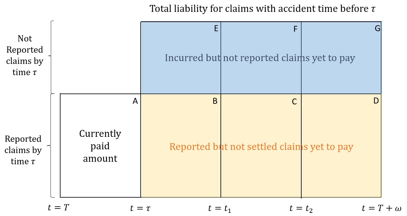
To illustrate the concept, let’s examine Figure 1. Combining all regions ( to ) yields the population discussed in Section 2, representing total liabilities. Focusing on the lower half of the figure, regions to , encompasses payments associated with reported claims at . Additionally, by narrowing our focus to the lower half of the figure and considering payments up to a specific time, such as (the union of regions , , and ), we obtain a truncated version of payments. Specifically, this includes total payments made for currently reported claims, excluding those made after . Note that the current paid amount is a sample from all of this subpopulation.
Adopting this approach, estimating the total liability for a specific subpopulation involves treating it as the main population from which current payments are sampled. Consequently, the IPW estimator, under a different sampling design, can be employed to estimate the liability. We refer to this approach as the “change of population principle”.
The different sample design under the change of population principle leads to different inclusion probabilities. Nevertheless, these probabilities can be easily determined using elementary conditional probability arguments. Specifically, when we limit the analysis to a subpopulation , we denote the inclusion probability under this restriction as . This probability represents the likelihood of payment being reported at , given its membership in subpopulation . Note that these probabilities differ in meaning and in value to those defined in Section 2. Bayes’ rule allows expressing this probability as
where denotes the probability of payment being sampled in subpopulation according to the original sampling design, which is influenced by factors like reporting delay and claim evolution. It is important to note that in this context, we assume the subpopulation is a subpopulation encompassing the current payments (region in Figure 1).
We will observe that for the reserves of interest, these probabilities can be straightforwardly expressed in terms of the probabilities associated with the previously defined delay time random variables and . Therefore, no additional estimations are necessary.
3.2 Calculation of the RBNS reserve
The Reported But Not Settled (RBNS) reserve represents payments that are yet to be made for claims already reported at valuation time . This reserve corresponds to the combined regions B, C, and D in Figure 1.
To estimate the reserve, we apply the change of population principle and define the population as the total payments associated with reported claims at . This population corresponds to the lower half of Figure 1, specifically . In reserving terminology, this corresponds to the ultimate of incurred losses for claims reported prior to .
Next, we determine the inclusion probabilities. The selection of the subpopulation depends on claim reporting, which occurs with probability . Utilizing the previously mentioned result derived from Bayes’ rule, the new inclusion probabilities for this population are
This result is intuitive since the region only considers claims already reported at , and the remaining randomness pertains to the evolution of payment occurrences only. Consequently, we can utilize the IPW estimator to obtain an unbiased estimator for the total payments of reported claims as
Hence, the RBNS reserve of interest can be obtained by subtracting this quantity from the current paid amount:
| (7) |
3.3 Calculation of the pure IBNR reserve
To estimate the Incurred But Not Reported (IBNR) reserve, we cannot directly apply the change of population principle since the current paid amount is not a subpopulation of the not reported claims population (Figure 1). However, we can easily overcome this by considering the current paid amount as the difference between two populations: the total payments (all regions in Figure 1) and the total payments of currently reported claims (lower half of Figure 1). Estimations for the liabilities associated with these populations have been discussed in Sections 2 and 3.2, respectively. Therefore, the IBNR liability can be estimated as the difference between these two estimations.
| (8) |
We would like to highlight that this approach to estimating the IBNR is analogous to the conventional actuarial method using run-off triangles, where the total reserve is estimated using the incurred claims triangle and subtracting the reserve obtained from the paid claims triangle. Unlike aggregate approaches that may yield negative reserve estimates, our method ensures non-negative estimations.
3.4 Calculation of cumulative and incremental payments
The estimator we have presented so far provides the ultimate amount of liabilities, but insurance companies require projections of the reserve payments over specific periods. These payments, known as incremental claims, can be estimated within our framework as follows: we utilize the change of population principle to estimate cumulative claims for different periods and then calculate the incremental claims as the difference between these cumulative claims. Notably, our model is continuous rather than discrete, allowing for the accommodation of any desired periodicity for incremental claims. We will illustrate this process for the total reserve only, however, it can be similarly applied to the RBNS.
Let’s consider an insurance company assessing claims incurred before the valuation time and interested in estimating the incremental claims associated with a future period between and (), denoted as . Visually, corresponds to and in Figure 1.
We start by considering the population of cumulative claims up to time , where only payments made up to are included i.e (regions , , and in Figure 1). Using the change of population principle, a payment belongs to this population if its payment time is before , which occurs with probability . Thus, the inclusion probability is:
and so the IPW estimator for cumulative claims is given by
| (9) |
The incremental claims between and are then given by , and so an unbiased estimator for incremental claims is
| (10) |
This is a very intuitive expression: The denominator, , scales the observed claims to the total amount, while the difference in probabilities in the numerator, , captures the proportion of the total observed between and .
3.5 Others applications
The IPW framework and the change of population principle extend beyond the reserves discussed thus far, allowing for the estimation of other types of reserves based on the specific needs of the actuary. For instance, the incurred but not paid (IBNP) reserve can be estimated as a portion of the current RBNS estimation. In this case, the payments themselves serve as the population for analysis using the change of population principle, with an inclusion probability linked to the occurrence of the first payment in the sequence.
Another example, though less explored, is the unearned premium reserve (UPR). This reserve pertains to payments for claims where the accident occurs after the valuation time , but only for policies in force at . To estimate the UPR, the change of population principle can be applied by defining a larger superpopulation consisting of all payments associated with claims from policies in force at , regardless of when the accidents occurred.
Finally, it is important to note that the IPW framework provides estimations without assuming specific meaning for . The quantity of interest represented by can be diverse as to the need of the actuary. For example, setting provides an estimation of the number of payments. Alternatively, the actuary can define as fees, commissions, policy management costs, etc., enabling a cost decomposition analysis of the reserve estimates.
4 Estimation of the model
In order to implement the IPW estimator, the key input required is the unknown inclusion probabilities . These probabilities are associated with the evolution of a claim, including reporting and settlement delays and depend on various attributes of the payment, the claim, and the policyholder, denoted as , as well as the claim amount itself. In this section, we outline a data-driven approach to estimating these values. As explained in Section 2, the inclusion probabilities consist of two separate components: the probability of reporting and the probability of settlement. Each one is estimated separately, so we discuss different strategies in Sections 4.1 and 4.2.
4.1 Estimation of the reporting delay times probabilities
To estimate probabilities, it is common to assume that the reporting delay times, conditioned on claim attributes , follow a common distribution function (see, for example, Verrall and Wüthrich, (2016)), that we will denote with and that will be the target of estimation in some type of regression framework to include the dependence on covariates.
The variable of interest, , is a time-to-event random variable commonly studied in survival modeling. Therefore, existing approaches in survival modeling can be utilized to estimate the overall distribution function and the desired probabilities. Proportional hazard models, also known as Cox regression models have been widely studied for this purpose in the statistical literature (e.g George et al., (2014)). These methods aim to directly model the log-hazard function of the random time variable, while accounting for the attributes in the modeling using a linear regression-like model
| (11) |
where, represents the baseline hazard function, which can be chosen from a parametric family or modeled nonparametrically e.g. using B-spline representation. represents the regression formula involving the covariates with corresponding regression parameters , and captures unobserved effects as an error term, also known as a random effect or frailty. Depending on the analysis, various structures for the random effect can be considered, such as autoregressive structure to capture trends and dependencies over time, or correlated effects to account for dependencies between claims that evolve together. Further guidance on specifying models for the hazard function can be found in Argyropoulos and Unruh, (2015).
Consequently, the desired probability is derived using the relationship
| (12) |
A crucial aspect in the estimation of the model above is accounting for the right truncation of the data. Indeed, due to the delay in the reporting times, our observations are limited to the conditional random variables: , and ignoring this fact would result in a downward bias in the overall distribution. Fortunately, the literature on survival analysis has widely explored this issue and provided solutions that the user can adopt for the estimation of the model. See for e.g Dempster et al., (1977), Gui and Li, (2005), Verbelen et al., (2015), Shakur et al., (2021), Fung et al., (2022)).
It is worth noting that not all survival models use linear regression structures or aim to describe the hazard function, and alternative approaches can offer different and flexible structures inspired by the machine learning literature. For instance, Wiegrebe et al., (2023) consider non-linear regression on covariates via deep learning approaches, Fung et al., (2022) propose a flexible model based on mixture of experts, and other approaches utilize survival trees such as Bou-Hamad et al., (2011). These alternatives provide increased flexibility compared to proportional hazard models, but may require additional expertise for model fitting and interpretation. The choice of the model must be achieved in a data-driven fashion aiming for the best fit to the data. Regardless of the methodology, careful consideration should be given to estimation under the right truncation of the data.
Lastly, due to the popularity of survival analysis in statistics applications, most of the methods described above have already been implemented in statistical software packages and are readily available for its use in our applications. For example, in R, there are various implementations, including Cox models as in Bender et al., (2018), mixture of experts as in Tseung et al., (2021), and deep survival models, survival trees, forests, and more in Sonabend et al., (2021).
4.2 Estimation of the payment times probabilities
Similarly to the previous case, we assume that the payment times, conditioned on claim attributes (including the reporting delay time ), follow a common distribution function denoted as that we aim to estimate via a regression framework. We will denote with to the maximum settlement time of a claim. While estimating this probability might seem similar to the previous case, a significant difference arises due to the recurrent nature of payment events for a given claim, as opposed to the one-time event of claim reporting. This recurrent event process (e.g. Cook et al., (2007)) necessitates an appropriately adapted modeling approach. This section will discuss two closely related, yet distinct approaches, to address this estimation.
Counting processes
Recurrent events are closely related to counting processes, where the former focus on event times and the latter on the number of events. In our case, we can consider the number of payments over time to be governed by a stochastically defined point process. Numerous works in insurance have explored modeling such processes in the context of reserving (e.g Antonio and Plat, (2014), Maciak et al., (2021), Yanez and Pigeon, (2021)).
Let’s define , where , as the counting process associated with the number of payments for a single claim. This is the counting process associated with the payments times for a given claim. For the sake of readability, we will omit the dependence on covariates in the notation, although it is important to acknowledge that all these quantities are dependent on them.
Since our objective is to determine probabilities of the form , our goal is to express the desired probability in terms of the process . To do so, we work with the reversed time version of the counting process where the new time is defined as . The reversed time process can be seen as a mortality process (see for e.g. Hiabu, (2017)), where the initial number of lives is and the lifetime random variable of a newborn follows the same distribution as . Then
| (13) |
where the second last equality holds by the traditional life table relationship , and the last equality is the tower property of conditional expectations.
Equation 13 reveals that the desired probability possesses an intuitive expression associated with the evolution of a claim up to settlement. In essence, the right-hand side of Equation (13) represents the expected proportion of payments made by time out of the total of payments. Another equivalent interpretation of this quantity is as the inverse of a development factor for the number of payments from time to the ultimate value at time . It is worth noting that this expression can be analytically computed only for certain processes. One such example is the widely used Poisson process (and some extensions), as illustrated in Example 1.
Example 1.
Suppose the is a non-homogeneous Poisson process with intensity rate , then
where we use the fact that in the third equality.
Along those lines, the actuary must select in a data-driven fashion an appropriate counting process (that incorporates the use of attributes) to model the number of payments per claim, and then proceed to compute the desired probability using Equation (13). Fitting counting processes could be a complex task and can vary depending on the approach used. For a comprehensive discussion on this matter, we refer to Andersen et al., (1985).
Reversed time counting process
By reversing the time of the counting process for the number of payments using the transformation , we can interpret the resulting process as a mortality process, as discussed by Hiabu, (2017). This analogy allows us to describe using a mortality model, which simplifies the fitting of the counting process. Reversing the time is a well-studied approach in the survival modeling literature Klein and Moeschberger, (2003).
Most mortality models belong to the class of survival models, and so can be embedded into the framework described in Section 4.1. The advantage of working with the reversed time process and mortality models over counting processes is the wider range of options available in terms of statistical modeling, as explored in the literature.
In this case, we assume that the reversed hazard function ( e.g Block et al., (1998)) of the time random variable , denoted as , is described using a Cox regression-like model that incorporates attribute information
As before, represents a baseline reversed hazard function, represents a regression formula involving the covariates with parameters , and represents a random effect. This modeling approach is analogous to the one described in Section 4.1, so we refer the reader to it.
As a result, the desired probability can be derived as:
| (14) |
Similar to the case of the reporting delay time, we face a right truncation problem when considering payments occurring after the valuation date. However, when reversing the time, this issue transforms into a left truncation problem and observations are only available if . Therefore, it is important to estimate the survival model for the reversed time random variable using an algorithm that allows for the left truncation of the data. Fortunately, modern implementations of survival models often include this capability as discussed in Section 4.1.
4.3 Goodness of fit and other considerations
Since the inclusion probabilities are the sole inputs for the IPW estimator, it is essential to have a well-fitted model for optimal performance. In this section, we discuss the assessment of the model’s goodness of fit using pseudo residuals. Additionally, we comment on the possible instability of the resulting IPW estimator and discuss ways of addressing such an issue.
Pseudo-residuals
One approach to assess the accuracy of the fitted distributions is to use uniform pseudo-residuals based on the probability integral transform (Rüschendorf, (2009)). These pseudo-residuals are constructed by evaluating the fitted distribution function at the observed values. They are widely used for goodness of fit assessment in various model families (e.g Buckby et al., (2020)). Considering that the observations come from a truncated distribution, the truncated version of the distribution should be taken into account. These pseudo residuals can be expressed as:
The uniform pseudo-residuals should exhibit approximate uniformity if the fitted model adequately represents the data. The uniform pseudo-residuals can be transformed to the normal scale using the quantile function of the standard normal distribution, denoted as :
These transformed normal pseudo-residuals allow for easier visualization and detection of deviations from the expected distribution when compared with a uniform scale, nevertheless, they are equivalent. Note that the Cox-Snell residuals, commonly used in survival analysis, are obtained by employing the quantile function of an exponential distribution instead of the normal distribution. See for e.g Klein and Moeschberger, (2003).
The normal pseudo-residuals can be utilized to assess the goodness of fit of the model through graphical analysis, such as scatter plots, etc, in the same fashion as with ordinary residuals in linear regression. The focus of the assessment is to determine whether the distribution of these residuals resembles a normal distribution, which can be achieved through QQ and PP plots, or hypothesis testing techniques.
Adjustments to the IPW estimate
A key issue that makes the claim reserving estimation process to be a very challenging one, is that the inclusion probabilities can vary significantly impacting the stability of the estimator. An extreme case is when the estimated inclusion probability of a claim is close to 0, which mostly occurs when a claim is recently reported, which represents the majority of the claims included in the IBNR reserve. Such circumstances can lead to instability in the estimator, potentially resulting in abnormally high values of the reserve when compared with experience on previous reserving exercises. This behavior has been widely documented in the survey sampling literature of the HT estimator. See for e.g., Hulliger, (1995), Chen et al., (2017) and references therein.
Trimming the inclusion probabilities is a method proposed to address the behavior of such extreme values. In this approach, if the inclusion probability is too small, it can be replaced with a larger value to get rid of the instability (Chen et al., (2017)). For reserving applications, the probabilities can be trimmed by artificially assuming a slightly later valuation date, which would increase the inclusion probabilities. Alternatively, data-driven methods, such as the algorithm 1 proposed by Zong et al., (2018), illustrated below, offer a more systematic approach. They showed that the mean square error of the IPW estimator is less or equal to its counterpart when such an adjustment is performed.
Obtain the ordered inclusion probabilities from smallest to largest.
for do
It is important to note that replacing the inclusion probabilities with larger values may introduce a downward bias in the reserve estimation. Therefore, it is recommended to perform any adjustment only if the estimation displays sensitivity to the changes in the inclusion probabilities. Indeed, if the estimation remains nearly unchanged after adjustments, retaining the original estimation would be preferred over the trimmed one.
5 Numerical study with real data
In this section, we showcase the application of the IPW estimator using a real data set obtained from a European automobile insurance company. The data-set comprises information on Body Injury (BI) claims from January 2009 to December 2012.
In line with our methodology’s primary objective of serving as an alternative to traditional macro-level models, while being simpler than fitting a micro-level model, we maintain a simplified approach to emphasize the practicality of the method in real-world applications.
5.1 Description of the data
The dataset contains detailed information about claim settlements, policyholder attributes, and automobile characteristics within the aforementioned time period. This information encompasses factors such as car weight, engine displacement, engine power, fuel type (gasoline or diesel), car age, policyholder age, and region (a total of five regions). Furthermore, the dataset includes details related to the accidents themselves, such as the time of occurrence and the type of accident (type 1 and type 2). Additionally, information regarding the progression of claim payments is available, including reporting time, settlement amounts, and the corresponding occurrence times.
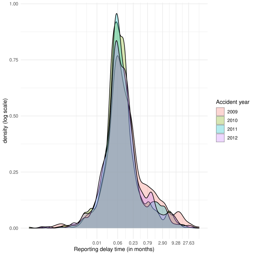
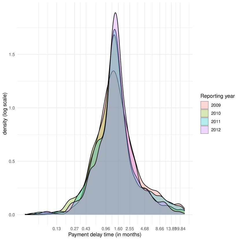
Our statistical modeling study focuses on the evolution of claims, specifically related to reporting delay time and payment times. We illustrate some characteristics of these quantities, such as the distributions in Figure 2 and summarize key statistics in Table 1.
| Variable | Year | Mean | Std. Dev. | Min. | 1st Qu. | Median | 3rd Qu. | Max. |
|---|---|---|---|---|---|---|---|---|
| 2009 | 1.03 | 4.09 | 0.00 | 0.05 | 0.10 | 0.28 | 43.28 | |
| Reporting | 2010 | 0.45 | 1.85 | 0.00 | 0.04 | 0.07 | 0.13 | 25.66 |
| delay time | 2011 | 0.50 | 2.16 | 0.00 | 0.04 | 0.07 | 0.17 | 24.09 |
| 2012 | 0.57 | 2.34 | 0.00 | 0.04 | 0.08 | 0.18 | 32.69 | |
| 2009 | 3.32 | 7.04 | 0.10 | 0.93 | 1.43 | 2.52 | 48.05 | |
| Payment | 2010 | 2.31 | 4.37 | 0.04 | 0.81 | 1.31 | 1.92 | 35.37 |
| delay time | 2011 | 2.82 | 5.41 | 0.03 | 0.91 | 1.41 | 2.14 | 35.38 |
| 2012 | 2.49 | 4.95 | 0.04 | 0.98 | 1.44 | 2.14 | 40.23 |
Upon reviewing the information presented in Figure 2 and Table 1, it is evident that the reporting delay tends to be relatively short, with an average duration of less than a month. However, there is notable variability in the tail behavior of this variable. In contrast, the progression of claim payments typically spans a few months on average, but there are instances where settlement times can extend over several years. It is important to note that the distributions of these variables exhibit complexities that are challenging to capture using simple parametric models. Specifically, they display significant temporal fluctuations, indicating that historical data may not adequately represent future events. To account for this, we define the maximum development time for future analysis as months, with approximately 99.95% of claims being settled within this timeframe.
5.2 Fitting of survival models
To model the reporting delay time, we employ a Cox regression-type model, as outlined in Section 4.1. Likewise, we adopt the reversed-time approach discussed in Section 4 to develop a model for claim evolution. As the maximum development time is 24 months, then the time window from 2009 to 2010 can be only used for training purposes, while the time window from 2011 to 2012 will be used for testing.
For the sake of illustration, we calculate reserves on a monthly basis i.e. several valuation dates each one month apart from the other. To ensure that the estimation captures the most recent evolution of claims as much as possible, we re-fit the models employing a rolling window approach, where only the last two years of data preceding a valuation date are used for the fitting. This approach aligns with the practices employed by industry professionals in their daily work. We do not consider a time-series model via correlated frailties due to the short time window of the training sets i.e only 2 years. Although there may be some variations in model parameters across different dates, the overall fit behaves similarly across time. We proceed to present the fitting processes for only the first valuation date in the testing period.
Reporting delay time
For the reporting delay time, , we fit a Cox regression model as in Equation (11) using the attributes of the policyholder as covariates:
For the sake of interpretability, we work with the standardized version of the continuous covariates. The baseline hazard function, denoted as , is estimated using a B-Spline representation. Additionally, we incorporate a non-linear effect of the covariate “Accident-day” with the term , which is also estimated using a B-Spline representation. This inclusion of a non-linear effect associated with calendar time provides the model with a dynamic alike structure, allowing it to account for some temporal changes.
To estimate the parameters while considering the right truncation of the data, we utilize a generalized additive model implementation via the piece-wise exponential modeling approach, as described by Bender et al., (2018). This approach is available in R packages such as flexsurvreg, pammtools or GJRM. The results of the estimation are presented in Table 2 and Figure 3.
| Coefficient | |||||||
|---|---|---|---|---|---|---|---|
| Value | |||||||
| Std. Err. | |||||||
| p-val |
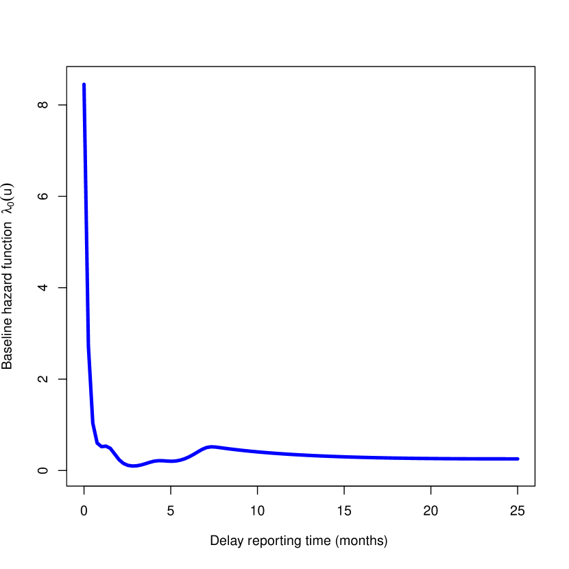
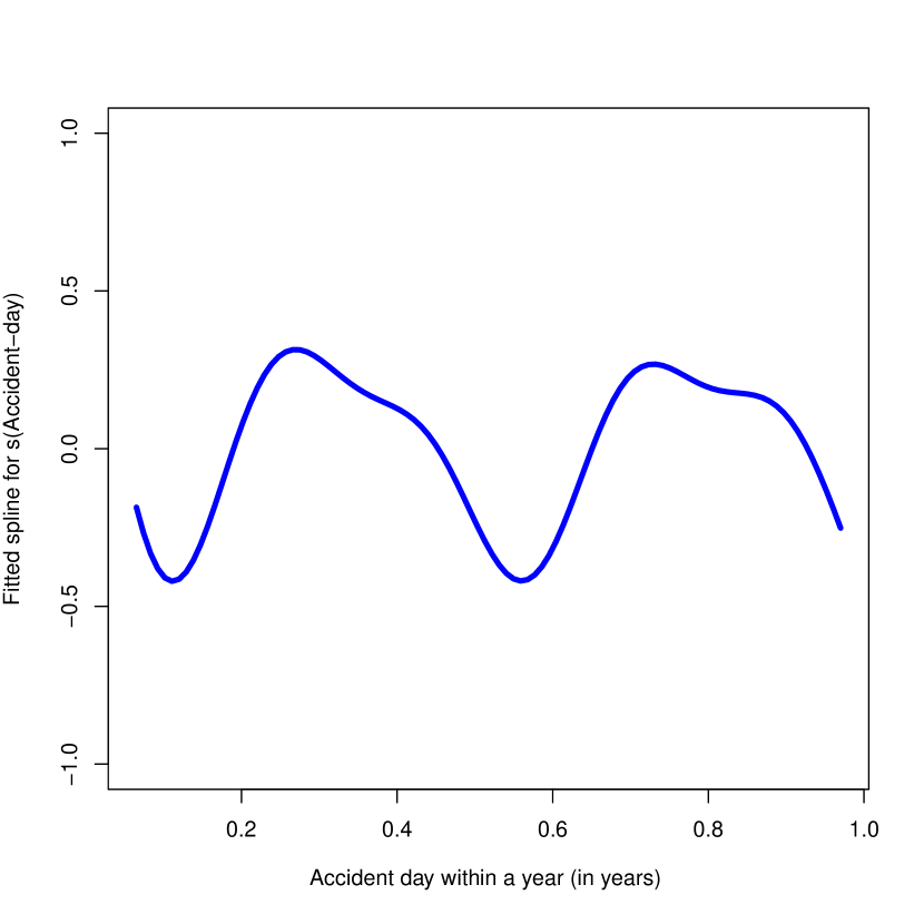
Table 2 shows that all the policyholder attributes included in the model are statistically relevant to describe the behaviour of the reporting delay time. The same conclusion applies to the categorical variable “Region”, although the detailed results are not presented in the table due to its numerous categories. The right panel of Figure 3 illustrates the non-linear effect associated with the accident day within a year. Time 0 is the beginning of the year i.e. January 1 and time 1 indicates the end of the year i.e. December 31. We can appreciate a quarterly seasonal pattern. Specifically, the hazard rate for the reporting delay time is higher in the second and fourth quarters compared to the other two quarters. Furthermore, the left panel of Figure 3 displays the baseline hazard function, indicating a large hazard rate during the initial months, suggesting a concentration of reporting delays within this period. The hazard rate then decreases rapidly but remains nonzero for large delay times, indicating a heavy tail.
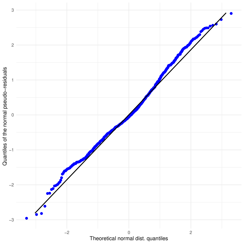
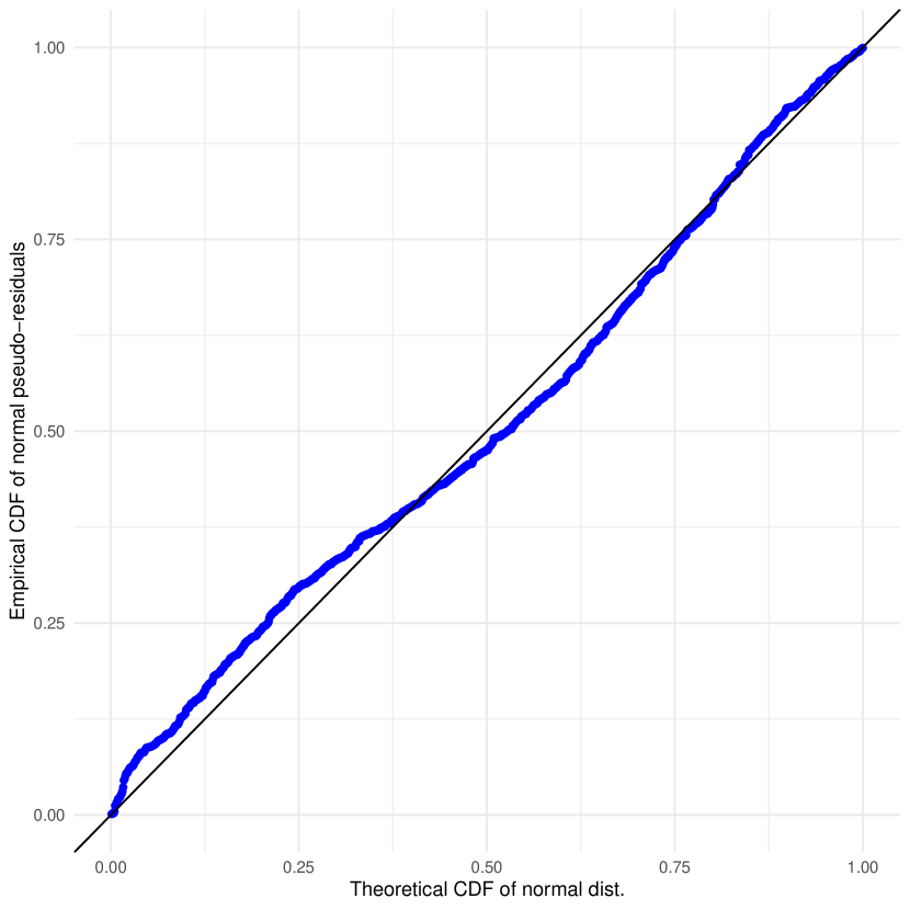
To assess the adequacy of the model fit, we employ normal pseudo residuals, as introduced in Section 4.3. Figure 4 presents QQ and PP plots, comparing these normal pseudo residuals against the theoretical normal distribution. From both plots, it is evident that the normal pseudo residuals exhibit no significant deviations from their expected theoretical counterparts. Hence, there is no evidence suggesting a lack of fit in the fitted distribution function.
Payment delay time
Next, we present the model for claim evolution utilizing the reversed time-counting process estimation approach, in conjunction with a Cox regression model similar to the one previously described. In this case, we consider a maximum settlement time of months, as mentioned earlier, and proceed to model the reversed time random variable . The Cox regression model for the reversed hazard function is defined as follows:
Once again, we work with the standardized version of the continuous covariates for interpretability. The baseline reversed hazard function, denoted as , is estimated using a B-Spline representation. The non-linear effects of the covariate “Reporting-day” are captured through the term , also estimated using a B-Spline representation.
This modeling approach mirrors the methodology presented in the previous section, and thus, we refrain from delving into further details. However, we highlight two key distinctions in this regression model. Firstly, we incorporate the reporting day as a non-linear effect aiming to capture time-related effects. Secondly, we include the observed reporting delay time as a covariate. We remark that these probabilities are based on all the information available at the payment time, which encompasses any additional information obtained during the reporting process.
| Coefficient | ||||||||
|---|---|---|---|---|---|---|---|---|
| Value | ||||||||
| Std. Err. | ||||||||
| p-val |
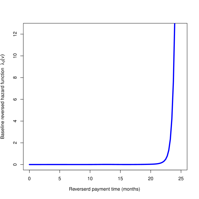
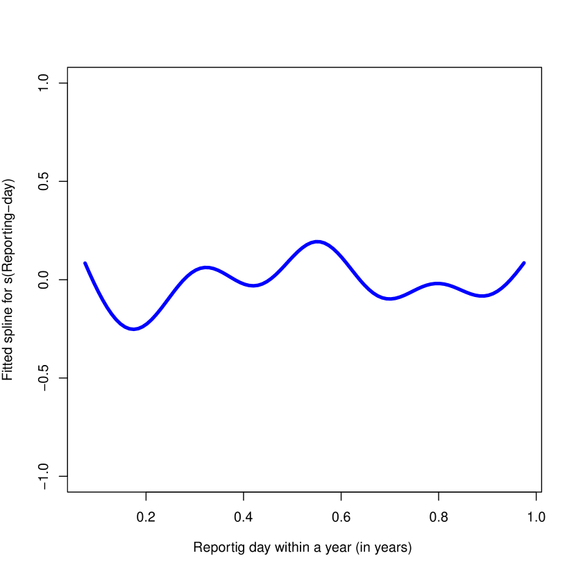
The fitted model is presented in Table 3 and Figure 5. The results exhibit similarities to the previous case, as shown in Table 3, where all policyholder attributes included in the model are statistically significant in describing the behavior of the reversed payment time. The right panel of Figure 5 displays the non-linear effect associated with the reporting day, indicating a quarterly seasonal pattern. However, the pattern is not as distinct as observed for the reporting delay time. The right panel of Figure 5 illustrates the baseline reversed hazard function, which should be interpreted in reverse. In this plot, time 0 and 24 months correspond to time 24 and time 0 months, respectively in the original scale. It is evident that the hazard function is initially high during the first couple of months (in the original scale), implying a significant number of payments occurring within this period. Subsequently, the hazard rate decreases rapidly, approaching zero, indicating the occurrence of some payments after several months from reporting.
To assess the goodness of fit, we employ again the normal pseudo residuals and validate them accordingly. Figure 6 displays QQ and PP plots, comparing these normal pseudo residuals against the theoretical normal distribution. Similar to the previous analysis, there is no significant deviation observed between the normal pseudo residuals and their expected theoretical counterparts in both plots. Hence, there is no evidence indicating a lack of fit in the fitted distribution function.


5.3 Estimation of the reserve for a single date
Here we show the estimation of the outstanding claims (IBNS), RBNS and IBNR reserves for the first date of the testing period. To ease the visualization and comparison, we present the estimation of the reserves in the classical run-off triangle format in Tables 5 and 6, yet however, recall that our method doesn’t rely on a given periodicity for its calculation or the construction of a triangle.
The inclusion probabilities and for the outstanding not settled claims are estimated directly from the models from the previous section using Equations (12), (14) and (1). Figure 7 displays the histogram of such probabilities and Table 4 displays some summary statistics. Briefly, we observe that the inclusion probabilities vary drastically from one claim to another due to the heterogeneity of the claims. Note that the probabilities tend to be closer to 1 than to 0 due to the low average reporting delay and payment time, and therefore only the most recently reported claims have a small probability.
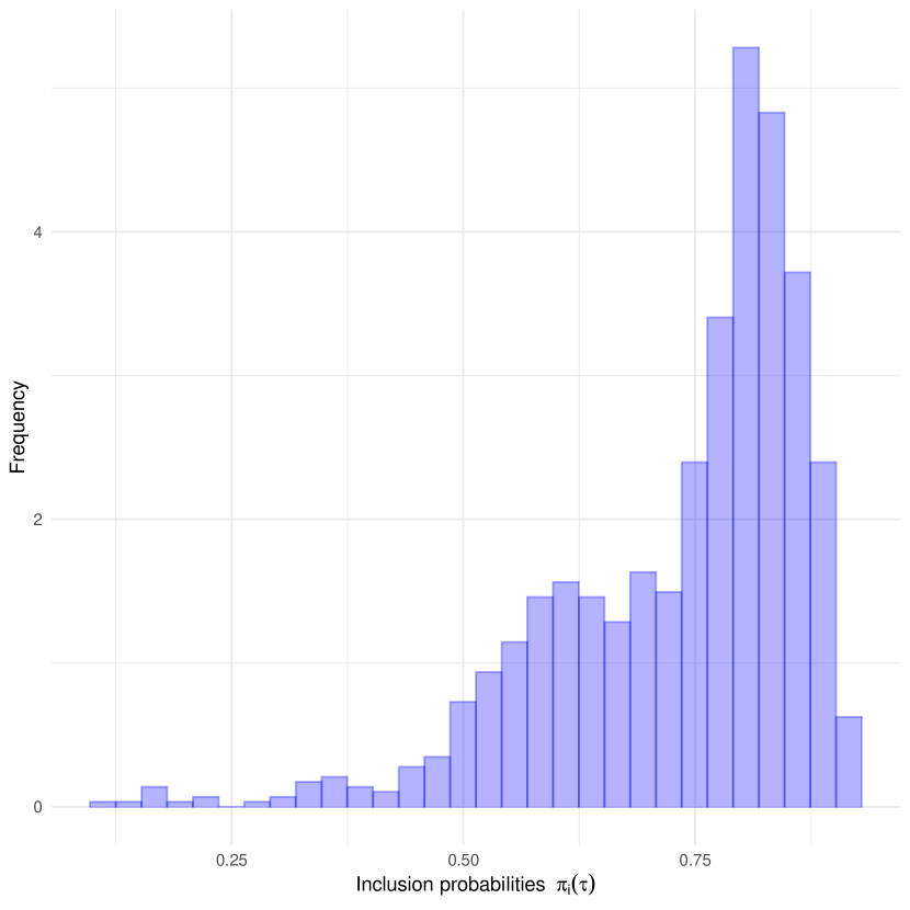
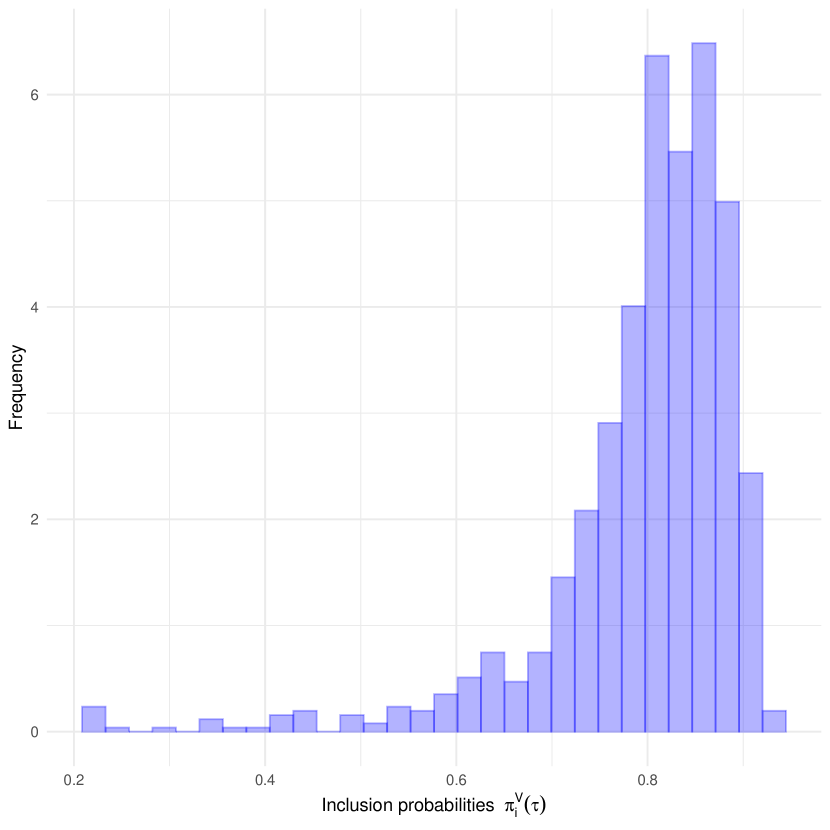
| Probability | Min. | 1st Qu. | Median | Mean | 3rd Qu. | Max. |
|---|---|---|---|---|---|---|
| 0.116 | 0.653 | 0.781 | 0.736 | 0.833 | 0.921 | |
| 0.216 | 0.766 | 0.820 | 0.797 | 0.860 | 0.927 |
Tables 5 and 6 present cumulative run-off triangles for total outstanding claims and reported but not settled claims, respectively, as of the valuation date. The incurred but not reported claims reserve estimation is derived from the difference between these triangles, which is not shown to avoid redundancy. We completed the lower half of the triangles using the true reserve values, the IPW estimator (using Equation (9)), and the Chain-Ladder method, on a monthly basis, for comparison purposes. To maintain readability and practicality, the table is limited to 13 months, representing approximately 98% of settled claims within this period. To differentiate between the RBNS and IBNR claims components in the Chain-Ladder method, we utilize the double Chain-Ladder method (Martínez-Miranda et al., (2012)).
Analyzing the lower half of the triangles in Tables 5 and 6, we observe that the IPW estimator provides cumulative payment estimations that exhibit similar trends and magnitudes as the actual cumulative claims. No evident patterns of under or over-estimation are observed. Additionally, the IPW estimator exhibits different behavior to the Chain-Ladder method, indicating the impact of using the individual level information in the estimation.
| M | 1 | 2 | 3 | 4 | 5 | 6 | 7 | 8 | 9 | 10 | 11 | 12 | 13 | ULT |
|---|---|---|---|---|---|---|---|---|---|---|---|---|---|---|
| 28,059 | ||||||||||||||
| 32,170 | ||||||||||||||
| 1 | 14,134 | 14,134 | 20,211 | 20,211 | 26,314 | 27,371 | 27,371 | 27,371 | 28,059 | 28,059 | 28,059 | 28,059 | 28,059 | 29,864 |
| 266,273 | 268,401 | |||||||||||||
| 268,495 | 323,763 | |||||||||||||
| 2 | 30,727 | 177,519 | 177,519 | 220,701 | 239,987 | 260,631 | 262,010 | 262,010 | 262,010 | 264,832 | 266,273 | 266,273 | 266,369 | 285,454 |
| 247,039 | 247,908 | 297,541 | ||||||||||||
| 249,269 | 272,571 | 309,415 | ||||||||||||
| 3 | 87,856 | 158,587 | 170,758 | 170,758 | 231,602 | 231,602 | 235,675 | 235,675 | 247,039 | 247,039 | 247,039 | 247,265 | 252,047 | 270,071 |
| 289,410 | 290,675 | 290,675 | 297,467 | |||||||||||
| 291,061 | 308,302 | 320,097 | 360,788 | |||||||||||
| 4 | 164,017 | 205,623 | 248,124 | 264,613 | 264,613 | 282,013 | 286,108 | 286,108 | 286,108 | 289,410 | 289,716 | 294,460 | 299,458 | 320,600 |
| 320,340 | 322,591 | 322,591 | 322,591 | 332,056 | ||||||||||
| 322,443 | 355,560 | 373,943 | 388,044 | 435,457 | ||||||||||
| 5 | 119,065 | 225,436 | 279,176 | 296,804 | 300,808 | 306,261 | 314,102 | 314,102 | 320,340 | 320,489 | 325,380 | 330,774 | 335,167 | 358,063 |
| 181,229 | 212,492 | 212,492 | 212,639 | 212,639 | 257,430 | |||||||||
| 182,423 | 194,660 | 202,168 | 207,354 | 211,442 | 222,585 | |||||||||
| 6 | 12,518 | 99,082 | 146,828 | 156,780 | 167,589 | 169,668 | 170,493 | 181,229 | 181,283 | 182,229 | 184,534 | 187,098 | 190,504 | 204,108 |
| 245,323 | 273,696 | 273,696 | 278,910 | 294,019 | 294,909 | 346,304 | ||||||||
| 247,042 | 264,234 | 273,743 | 284,226 | 291,805 | 296,200 | 314,629 | ||||||||
| 7 | 37,174 | 132,479 | 209,631 | 218,619 | 232,507 | 241,423 | 245,323 | 245,494 | 254,273 | 255,601 | 258,672 | 262,410 | 267,209 | 286,328 |
| 285,608 | 290,118 | 295,826 | 296,713 | 312,941 | 312,941 | 315,764 | 321,604 | |||||||
| 290,212 | 327,506 | 346,422 | 369,539 | 389,189 | 398,289 | 408,089 | 442,873 | |||||||
| 8 | 40,234 | 191,089 | 227,720 | 241,797 | 285,608 | 285,608 | 286,667 | 293,846 | 302,802 | 304,561 | 308,474 | 312,988 | 318,639 | 340,750 |
| 229,304 | 233,399 | 234,422 | 234,592 | 235,953 | 235,953 | 258,863 | 259,236 | 782,474 | ||||||
| 232,096 | 257,759 | 272,238 | 285,793 | 324,709 | 344,994 | 374,998 | 386,755 | 434,518 | ||||||
| 9 | 14,251 | 123,802 | 176,626 | 217,705 | 229,304 | 230,700 | 234,301 | 239,968 | 247,470 | 248,875 | 252,014 | 255,766 | 260,134 | 278,538 |
| 372,005 | 408,322 | 411,377 | 413,752 | 413,806 | 415,288 | 417,411 | 417,411 | 417,411 | 483,132 | |||||
| 368,019 | 412,041 | 437,451 | 447,627 | 496,137 | 549,596 | 629,822 | 658,452 | 672,707 | 788,018 | |||||
| 10 | 22,408 | 188,162 | 274,916 | 363,112 | 367,423 | 385,109 | 390,692 | 399,462 | 413,096 | 415,207 | 421,599 | 428,037 | 434,747 | 465,082 |
| 312,148 | 324,473 | 345,710 | 409,621 | 424,520 | 426,909 | 426,909 | 427,083 | 435,422 | 436,328 | 454,346 | ||||
| 319,151 | 371,166 | 397,213 | 408,778 | 422,950 | 461,395 | 492,821 | 496,838 | 503,133 | 513,386 | 546,347 | ||||
| 11 | 22,017 | 256,833 | 312,025 | 315,773 | 337,649 | 354,696 | 359,395 | 367,446 | 380,638 | 382,364 | 387,143 | 392,530 | 400,024 | 428,665 |
| 157,762 | 258,713 | 281,683 | 286,280 | 291,383 | 291,383 | 310,758 | 329,514 | 329,940 | 346,858 | 348,634 | 359,294 | |||
| 114,398 | 172,447 | 195,043 | 204,176 | 217,368 | 245,751 | 282,399 | 287,515 | 290,146 | 295,399 | 300,999 | 321,814 | |||
| 12 | 11,371 | 105,591 | 109,022 | 125,655 | 134,820 | 140,940 | 143,118 | 146,415 | 151,346 | 152,163 | 154,078 | 156,346 | 159,074 | 170,367 |
| 35,614 | 169,336 | 194,656 | 207,267 | 230,055 | 245,208 | 249,372 | 249,372 | 249,372 | 249,372 | 250,671 | 250,671 | 250,922 | ||
| 30,208 | 78,756 | 96,315 | 102,162 | 119,705 | 138,875 | 168,485 | 172,777 | 174,132 | 176,301 | 178,786 | 181,360 | 190,887 | ||
| 13 | 24,662 | 24,662 | 64,017 | 69,236 | 72,943 | 74,363 | 75,853 | 78,469 | 79,224 | 80,102 | 81,156 | 82,654 | 83,441 | 88,919 |
| M | 1 | 2 | 3 | 4 | 5 | 6 | 7 | 8 | 9 | 10 | 11 | 12 | 13 | ULT |
|---|---|---|---|---|---|---|---|---|---|---|---|---|---|---|
| 28,059 | ||||||||||||||
| 32,048 | ||||||||||||||
| 1 | 14,134 | 14,134 | 20,211 | 20,211 | 26,314 | 27,371 | 27,371 | 27,371 | 28,059 | 28,059 | 28,059 | 28,059 | 28,059 | 29,744 |
| 266,273 | 268,401 | |||||||||||||
| 268,495 | 316,876 | |||||||||||||
| 2 | 30,727 | 177,519 | 177,519 | 220,701 | 239,987 | 260,631 | 262,010 | 262,010 | 262,010 | 264,832 | 266,273 | 266,273 | 266,352 | 283,936 |
| 247,039 | 247,908 | 295,920 | ||||||||||||
| 249,269 | 272,571 | 303,666 | ||||||||||||
| 3 | 87,856 | 158,587 | 170,758 | 170,758 | 231,602 | 231,602 | 235,675 | 235,675 | 247,039 | 247,039 | 247,039 | 247,233 | 251,331 | 267,896 |
| 289,410 | 290,675 | 290,675 | 296,975 | |||||||||||
| 291,061 | 308,302 | 320,097 | 335,713 | |||||||||||
| 4 | 164,017 | 205,623 | 248,124 | 264,613 | 264,613 | 282,013 | 286,108 | 286,108 | 286,108 | 289,410 | 289,716 | 294,290 | 298,562 | 318,018 |
| 320,340 | 322,591 | 322,591 | 322,591 | 332,056 | ||||||||||
| 322,443 | 355,527 | 373,910 | 383,230 | 402,049 | ||||||||||
| 5 | 119,065 | 225,436 | 279,176 | 296,804 | 300,808 | 306,261 | 314,102 | 314,102 | 320,340 | 320,456 | 324,742 | 329,669 | 333,381 | 354,482 |
| 181,229 | 212,492 | 212,492 | 212,639 | 212,639 | 257,430 | |||||||||
| 182,423 | 194,408 | 201,907 | 205,999 | 209,165 | 219,408 | |||||||||
| 6 | 12,518 | 99,082 | 146,828 | 156,780 | 167,589 | 169,668 | 170,493 | 181,229 | 181,265 | 181,933 | 183,790 | 186,288 | 189,194 | 201,648 |
| 245,323 | 273,696 | 273,696 | 278,910 | 282,049 | 282,049 | 333,444 | ||||||||
| 247,042 | 263,487 | 272,968 | 277,245 | 280,291 | 282,707 | 297,815 | ||||||||
| 7 | 37,174 | 132,479 | 209,631 | 218,619 | 232,507 | 241,423 | 245,323 | 245,468 | 252,902 | 253,831 | 256,254 | 259,887 | 263,961 | 281,367 |
| 285,608 | 290,118 | 295,826 | 296,713 | 310,655 | 310,655 | 313,478 | 319,318 | |||||||
| 290,212 | 327,506 | 346,422 | 354,353 | 358,311 | 360,353 | 362,343 | 391,250 | |||||||
| 8 | 40,234 | 191,089 | 227,720 | 241,797 | 285,608 | 285,608 | 286,252 | 291,115 | 298,601 | 299,853 | 303,047 | 307,302 | 312,034 | 332,059 |
| 229,304 | 233,399 | 234,422 | 234,592 | 234,592 | 234,592 | 257,501 | 257,874 | 259,624 | ||||||
| 232,096 | 257,759 | 272,238 | 277,845 | 279,895 | 280,390 | 281,496 | 284,773 | 309,678 | ||||||
| 9 | 14,251 | 123,802 | 176,626 | 217,705 | 229,304 | 230,261 | 232,668 | 236,447 | 242,690 | 243,679 | 246,201 | 249,730 | 253,379 | 269,920 |
| 372,005 | 407,354 | 410,409 | 412,784 | 412,838 | 414,320 | 416,443 | 416,443 | 416,443 | 438,292 | |||||
| 368,019 | 412,041 | 437,451 | 447,627 | 451,060 | 451,101 | 451,161 | 454,506 | 464,323 | 499,305 | |||||
| 10 | 22,408 | 188,162 | 274,916 | 363,112 | 366,874 | 378,973 | 382,687 | 388,215 | 399,427 | 400,865 | 406,052 | 411,896 | 417,404 | 444,322 |
| 312,148 | 324,473 | 340,741 | 404,394 | 419,293 | 421,682 | 421,682 | 421,856 | 424,104 | 424,104 | 439,958 | ||||
| 319,151 | 371,166 | 397,213 | 408,778 | 413,575 | 413,949 | 413,949 | 413,969 | 419,168 | 427,627 | 452,425 | ||||
| 11 | 22,017 | 256,833 | 312,025 | 315,615 | 336,465 | 348,095 | 351,263 | 356,156 | 366,992 | 368,139 | 371,767 | 376,883 | 383,052 | 408,325 |
| 157,762 | 258,713 | 280,666 | 284,373 | 288,514 | 288,514 | 303,401 | 314,932 | 315,358 | 322,242 | 324,018 | 333,471 | |||
| 114,398 | 172,447 | 195,043 | 204,176 | 208,635 | 209,811 | 209,811 | 209,812 | 211,616 | 215,341 | 219,281 | 231,872 | |||
| 12 | 11,371 | 105,591 | 108,806 | 124,708 | 133,214 | 137,359 | 138,795 | 140,870 | 144,880 | 145,436 | 146,924 | 149,019 | 151,245 | 161,149 |
| 35,614 | 169,336 | 184,855 | 193,175 | 193,175 | 205,684 | 209,848 | 209,848 | 209,848 | 209,848 | 209,848 | 209,848 | 210,100 | ||
| 30,208 | 77,486 | 94,635 | 100,349 | 103,022 | 103,997 | 104,078 | 104,140 | 104,880 | 106,127 | 107,566 | 109,055 | 113,674 | ||
| 13 | 24,662 | 24,662 | 61,364 | 66,154 | 68,776 | 69,700 | 70,561 | 72,564 | 73,113 | 73,740 | 74,677 | 75,884 | 76,486 | 81,161 |
The overall findings indicate that, at the cell level, the IPW estimator performs similarly to the Chain-Ladder method for the given valuation date. We do note that the IPW tends to better capture the changes in the reserve on the most recent dates as a result of accounting for the composition of the portfolio in the estimation. However, it is important to note that the IPW estimator does not consistently outperform the Chain-Ladder method in all cells of the triangle. We emphasize that, even though the IPW estimator can provide such estimations at the cell level, it may not possess the same precision as the estimation of the reserve as a whole. The more granular the desired estimation (i.e the smaller the subpopulation of interest), the lower the level of accuracy.
| Reserve Type | Method | Ultimate | Reserve | Error | % Error |
|---|---|---|---|---|---|
| IBNS | True value | 4,479,030 | 1,605,716 | - | - |
| IPW | 4,723,264 | 1,849,950 | -244,234 | -15.2% | |
| CL | 3,526,809 | 653,495 | 952,221 | 59.3% | |
| RBNS | True value | 3,813,048 | 939,733 | - | - |
| IPW | 3,905,779 | 1,032,465 | -92,732 | -9.9% | |
| CL | 3,434,026 | 560,712 | 379,022 | 40.3% | |
| IBNR | True value | 665,983 | 665,983 | - | - |
| IPW | 817,485 | 817,485 | -151,502 | -22.7% | |
| CL | 92,783 | 92,783 | 573,199 | 86.1% |
Along those lines, instead of focusing on cell-level comparisons, our emphasis lies now on the aggregation of cells to determine the actual reserve value, which is the ultimate objective of estimation. It is noteworthy that the IPW estimator directly provides an estimation of the total reserves using Equations (3), (7) and (8), eliminating the need for constructing the run-off triangle in comparison to the Chain-Ladder method. Table 7 presents the aggregated reserve values obtained by summing the ultimate values for each accident date, along with the corresponding estimation errors. Our findings reveal that the IPW estimator yields reserve values that closely align with their true counterparts for all reserve types, exhibiting significantly lower estimation errors compared to the Chain-Ladder method.
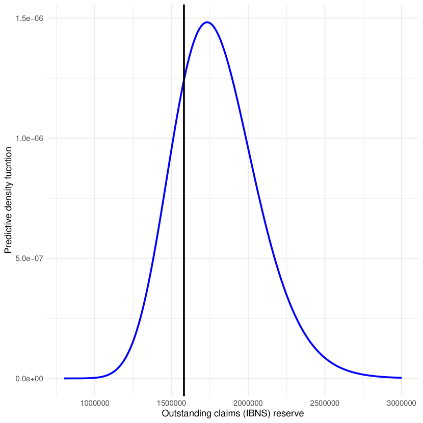
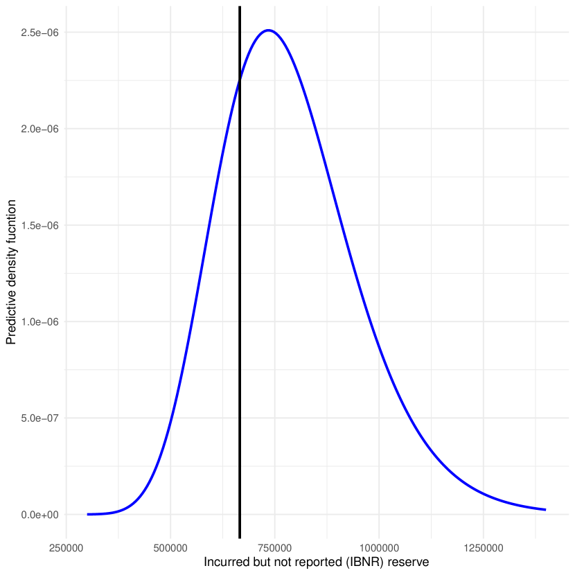
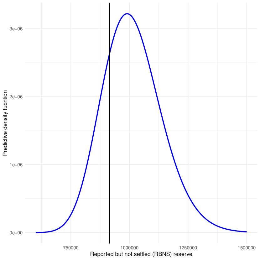
Furthermore, to evaluate the predictive quality of these estimates from a probabilistic standpoint, Figure 8 illustrates the predictive distribution of the reserves based on the sampling distribution of the IPW estimators, juxtaposed with the actual observed values. Notably, we observe that the true values consistently fall within the central region of the distribution, closely aligning with the corresponding modes, which represent the predicted reserve values. Consequently, the IPW-based predictions exhibit consistency with the observed reality.
5.4 Estimation of the reserve for several dates
Here we present the estimation of reserves for all 24 months in the testing period. Figure 9 illustrates the estimations for the outstanding claims compared to the true value of the reserve at the corresponding month. Additionally, Figures 10 and 11 depict the estimation for RBNS and IBNR, respectively. To provide a comprehensive analysis, we include 95% confidence intervals for the estimations and include Chain-Ladder (CL) method estimates for comparison. Furthermore, Table 8 presents error metrics to assess the disparities between the estimations across all dates. We would like to note that this kind of temporal analysis is often overlooked in the claim-reserving literature due to its inherent challenges for having consistent estimations. Our aim is not to boast about the complexity of the analysis but rather to show the behavior of the IPW method in distinct scenarios.
| Reserve Type | Method | ME | RMSE | MAE | MAPE |
|---|---|---|---|---|---|
| IBNS | IPW | 68,779 | 215,368 | 228,874 | 14% |
| CL | 540,239 | 662,345 | 574,588 | 40% | |
| RBNS | IPW | 183,197 | 189,087 | 228,939 | 17% |
| CL | 140,470 | 279,493 | 286,723 | 33% | |
| IBNR | IPW | -114,418 | 198,679 | 209,339 | 37% |
| CL | 399,769 | 328,503 | 399,769 | 76% |
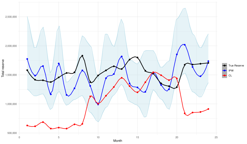
With respect to the total reserve, Figure 9 demonstrates that the IPW estimator produces predictions that closely align with the true value of the reserve for the majority of the observed periods, exhibiting no discernible pattern of under or overestimations. Additionally, the actual reserve value consistently falls within the associated confidence intervals, indicating a consistent fit with the predicted value. Notably, the IPW prediction proves to be more accurate than the traditional Chain-Ladder method during the considered period. This observation is further supported by the results in Table 8, where the error metrics for the IPW over the 24-month period outperform those of the Chain-Ladder method. Therefore, the IPW along with the use of individual information has more predictive power than the macro reserving method.
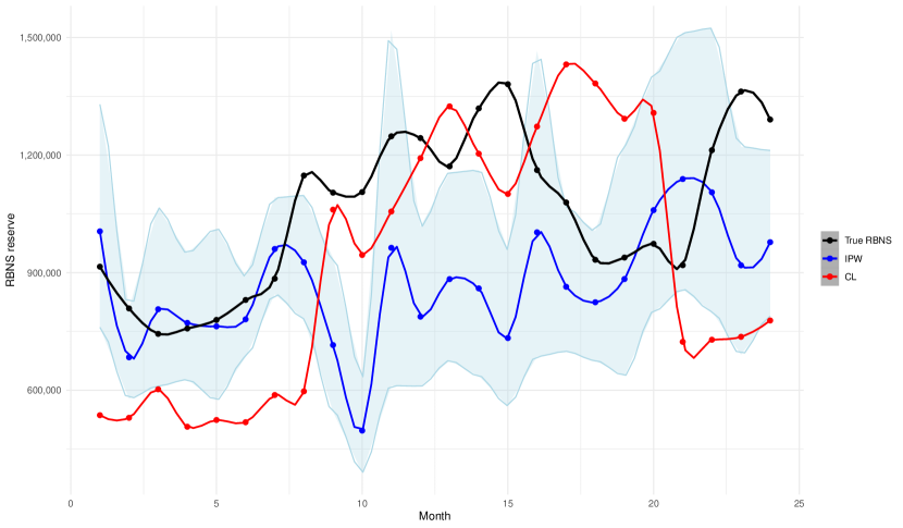
With respect to the RBNS, we observe in Figure 10 that the IPW estimator provides accurate predictions for the majority of the first year within the time window and for a portion of the second half of the second year. However, during the intermediate period (8th month to 17th month), the IPW underestimates the reserve, although some data points in this range still fall within the confidence band. It is worth noting that this period exhibits relatively higher reserve levels compared to the rest of the considered time window, which may be attributed to management-related actions of the insurance company that lead to larger reserves. In such cases, the IPW estimation takes longer to capture these changes, as the distribution estimation relies on the preceding two years of data. Consequently, it takes several months for the most recent data to have a significant impact on the estimation. On the other hand, the Chain-Ladder method appears to be more adept at capturing this particular change. However, outside of this specific period, the Chain-Ladder method demonstrates considerable underperformance. Despite this behavior, the IPW consistently outperforms the Chain-Ladder method on average throughout the entire period, as evidenced by the lower error metrics in Table 8.
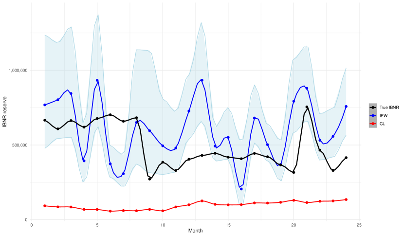
Finally, regarding the IBNR reserve, we observe in Figure 11 that the IPW estimator provides a reasonable estimation for almost the entire considered period, fluctuating around the true reserve. It is worth noting that the IPW estimator exhibits a more variable behavior compared to previous scenarios. This variability is expected because the IBNR, in our case, represents a smaller proportion of the subpopulation due to the relatively low reporting delay time. Generally, as the size of the subpopulation decreases, the estimation variance of the IPW increases. Despite this variability, the IPW estimator consistently outperforms the traditional Chain-Ladder method over the entire 24-month period, as indicated in Table 8. It is interesting to note that the IPW tends to follow the same trends observed in the true value of the reserve i.e. it has congruent patterns of fluctuations and variations in a comparable manner with the true value. We would like to note the fact that the Chain-Ladder estimation is stable throughout the period, while the IPW estimation is not. We attribute this behavior to the fact that the Chain-Ladder assumes a homogeneous portfolio while the IPW does not.
Observation 1.
We encountered instability in the behavior of the IPW estimator (i.e absurdly abnormal large reserves) when performing the estimation on some dates, along the same lines as the behavior described in Section 4.3. To address this issue, we implemented the adjusted version of the IPW estimator, as described in algorithm 1, and compared it to the raw IPW estimator. If the percentual difference between the two estimations exceeded a certain threshold (e.g., more than 3%), we retained the adjusted estimation. For cases where the difference was not significant, we kept the original estimation. As a result, the estimations become more stable across dates.
Note that one may work directly with the adjusted estimation, but it may introduce a systematic downward bias. Therefore, in practical applications, it is advisable to apply the adjustment only when the actuary considers it necessary.
6 Conclusions
Macro-level reserving models, particularly the Chain-Ladder method, overlook the underlying heterogeneity within the portfolio of policyholders, treating all claims equally, and providing most of the time modest estimations. Therefore, the estimation of the reserve does not benefit from the use of the individual attributes of the policyholders, which have been shown to provide a significant improvement in the accuracy of these methods in the literature of micro-level reserving.
In this paper, we address the limitation of macro-level reserving models by proposing a statistically justified macro-level reserve estimator based on Inverse Probability Weighting (IPW). Unlike traditional macro-level models, our method incorporates individual-level information in the weights to improve the accuracy of reserve estimation. Moreover, such incorporation is achieved within a less complex framework compared to micro-level models, in the sense that no explicit assumptions on claim frequency or severity are made.
The IPW estimator serves as a hybrid approach that bridges the gap between macro and micro-level methods. It assigns attribute-driven weights to each claim, allowing for a development factor specific to each claim’s settlement, similar to the familiar principles of the Chain-Ladder method when applied at the granular level. This method represents an initial step towards obtaining more precise reserves from macro-level models and serves as an intermediate stage in the development of a customized micro-level reserving model.
We believe that the IPW estimator offers a possibly seamless transition from macro to micro-level reserving for insurance companies. We hope practitioners find this method appealing as it is a natural extension of the traditional Chain-Ladder method, accounting for portfolio heterogeneity in a statistically justified fashion.
Future research should explore alternative approaches for estimation, potentially through the development of tailored models specifically designed for inclusion probabilities as in the development factor in Equation (13), which is simpler to interpret. Additionally, investigating the connection between claim reserving and population sampling techniques holds promise for further advancements in estimating reserves. We are currently engaged in related research, Calcetero-Vanegas et al., (2023), delving deeper into the implications of survey sampling theory on the claim reserving problem.
Acknowledgments
This work was partly supported by Natural Sciences and Engineering Research Council of Canada [RGPIN 284246, RGPIN-2017-06684]. Sebastián acknowledges the Mountain Pygmy Possum, an endangered species in Australia, for inspiring research on population sampling and also this project.
References
- Andersen et al., (1985) Andersen, P. K., Ørnulf Borgan, Hjort, N. L., Arjas, E., Stene, J., and Aalen, O. (1985). Counting process models for life history data: A review [with discussion and reply]. Scandinavian Journal of Statistics, 12(2):97–158.
- Antonio and Plat, (2014) Antonio, K. and Plat, R. (2014). Micro-level stochastic loss reserving for general insurance. Scandinavian Actuarial Journal, 2014(7):649–669.
- Argyropoulos and Unruh, (2015) Argyropoulos, C. and Unruh, M. L. (2015). Analysis of time to event outcomes in randomized controlled trials by generalized additive models. PLoS One, 10(4):e0123784.
- Arnab, (2017) Arnab, R. (2017). Survey Sampling Theory and Applications. Academic Press.
- Bender et al., (2018) Bender, A., Groll, A., and Scheipl, F. (2018). A generalized additive model approach to time-to-event analysis. Statistical Modelling, 18(3-4):299–321.
- Berger, (1998) Berger, Y. G. (1998). Rate of convergence for asymptotic variance of the horvitz–thompson estimator. Journal of Statistical Planning and Inference, 74(1):149–168.
- Block et al., (1998) Block, H. W., Savits, T. H., and Singh, H. (1998). The reversed hazard rate function. Probability in the Engineering and Informational Sciences, 12(1):69–90.
- Bou-Hamad et al., (2011) Bou-Hamad, I., Larocque, D., and Ben-Ameur, H. (2011). A review of survival trees. Statistics Surveys, 5:44 – 71.
- Boumezoued and Devineau, (2017) Boumezoued, A. and Devineau, L. (2017). Individual claims reserving: a survey. working paper or preprint.
- Buckby et al., (2020) Buckby, J., Wang, T., Zhuang, J., and Obara, K. (2020). Model checking for hidden markov models. Journal of Computational and Graphical Statistics, 29(4):859–874.
- Calcetero-Vanegas et al., (2023) Calcetero-Vanegas, S., Badescu, A., and Lin, S. (2023). A survey sampling theoretical framework for claim reserving. In preparation.
- Carrato and Visintin, (2019) Carrato, A. and Visintin, M. (2019). From the chain ladder to individual claims reserving using machine learning techniques. In ASTIN Colloquium, Cape Town, South Africa, April, pages 2–5.
- Chauvet and Vallée, (2018) Chauvet, G. and Vallée, A.-A. (2018). Inference for two-stage sampling designs with application to a panel for urban policy. working paper or preprint.
- Chen et al., (2017) Chen, Q., Elliott, M. R., Haziza, D., Yang, Y., Ghosh, M., Little, R. J. A., Sedransk, J., and Thompson, M. (2017). Approaches to improving survey-weighted estimates. Statistical Science, 32(2):227–248.
- Cook et al., (2007) Cook, R. J., Lawless, J. F., et al. (2007). The Statistical Analysis of Recurrent Events. Springer.
- Crevecoeur et al., (2022) Crevecoeur, J., Robben, J., and Antonio, K. (2022). A hierarchical reserving model for reported non-life insurance claims. Insurance: Mathematics and Economics, 104:158–184.
- Dempster et al., (1977) Dempster, A. P., Laird, N. M., and Rubin, D. B. (1977). Maximum likelihood from incomplete data via the em algorithm. Journal of the royal statistical society: series B (methodological), 39(1):1–22.
- Efron and Stein, (1981) Efron, B. and Stein, C. (1981). The jackknife estimate of variance. The Annals of Statistics, 9(3):586–596.
- Francis, (2016) Francis, L. (2016). Astin working party releases report on reserving practices for general insurance worldwide. https://ar.casact.org/astin-working-party-releases-report-on-reserving-practices-for-general-insurance-worldwide/. Accessed: 2023-06-04.
- Fung et al., (2021) Fung, T. C., Badescu, A. L., and Lin, X. S. (2021). A new class of severity regression models with an application to ibnr prediction. North American Actuarial Journal, 25(2):206–231.
- Fung et al., (2022) Fung, T. C., Badescu, A. L., and Lin, X. S. (2022). Fitting censored and truncated regression data using the mixture of experts models. North American Actuarial Journal, 26(4):496–520.
- George et al., (2014) George, B., Seals, S., and Aban, I. (2014). Survival analysis and regression models. Journal of nuclear cardiology, 21(4):686–694.
- Gui and Li, (2005) Gui, J. and Li, H. (2005). Threshold gradient descent method for censored data regression with applications in pharmacogenomics. Biocomputing 2005, 1:272–283.
- Hiabu, (2017) Hiabu, M. (2017). On the relationship between classical chain ladder and granular reserving. Scandinavian Actuarial Journal, 2017(8):708–729.
- Hulliger, (1995) Hulliger, B. (1995). Outlier robust horvitz-thompson estimators. Survey Methodology, 21(1):79–87.
- Klein and Moeschberger, (2003) Klein, J. P. and Moeschberger, M. L. (2003). Survival Analysis: Techniques for Censored and Truncated Data, volume 1230. Springer.
- Maciak et al., (2021) Maciak, M., Okhrin, O., and Pešta, M. (2021). Infinitely stochastic micro reserving. Insurance: Mathematics and Economics, 100:30–58.
- Mack, (1994) Mack, T. (1994). Which stochastic model is underlying the chain ladder method? Insurance: mathematics and economics, 15(2-3):133–138.
- Martínez-Miranda et al., (2012) Martínez-Miranda, M. D., Nielsen, J. P., and Verrall, R. (2012). Double chain ladder. ASTIN Bulletin: The Journal of the IAA, 42(1):59–76.
- Quarg and Mack, (2004) Quarg, G. and Mack, T. (2004). Munich chain ladder. Blätter der DGVFM, 26(4):597–630.
- Rüschendorf, (2009) Rüschendorf, L. (2009). On the distributional transform, sklar’s theorem, and the empirical copula process. Journal of statistical planning and inference, 139(11):3921–3927.
- Särndal et al., (2003) Särndal, C.-E., Swensson, B., and Wretman, J. (2003). Model Assisted Survey Sampling. Springer Science & Business Media.
- Schmidt, (2017) Schmidt, K. D. (2017). A bibliography on loss reserving. https://www.researchgate.net/profile/Klaus-Schmidt-6/publication/321369245_A_Bibliography_on_Loss_Reserving_Update_November_2017/links/5a1ef6f8458515a4c3d3b2ac/A-Bibliography-on-Loss-Reserving-Update-November-2017.pdf. Accessed: 2023-06-04.
- Shakur et al., (2021) Shakur, A. H., Huang, S., Qian, X., and Chang, X. (2021). Survfit: doubly sparse rule learning for survival data. Journal of Biomedical Informatics, 117:103691.
- Sonabend et al., (2021) Sonabend, R., Király, F. J., Bender, A., Bischl, B., and Lang, M. (2021). mlr3proba: an r package for machine learning in survival analysis. Bioinformatics, 37(17):2789–2791.
- Taha et al., (2021) Taha, A., Cosgrave, B., Rashwan, W., and McKeever, S. (2021). Insurance reserve prediction: Opportunities and challenges. In 2021 International Conference on Computational Science and Computational Intelligence (CSCI), pages 290–295.
- Taylor et al., (2008) Taylor, G., McGuire, G., and Sullivan, J. (2008). Individual claim loss reserving conditioned by case estimates. Annals of Actuarial Science, 3(1-2):215–256.
- Thompson, (2012) Thompson, S. K. (2012). Sampling, volume 755. John Wiley & Sons.
- Tseung et al., (2021) Tseung, S. C., Badescu, A. L., Fung, T. C., and Lin, X. S. (2021). Lrmoe. jl: a software package for insurance loss modelling using mixture of experts regression model. Annals of Actuarial Science, 15(2):419–440.
- Verbelen et al., (2015) Verbelen, R., Gong, L., Antonio, K., Badescu, A., and Lin, S. (2015). Fitting mixtures of erlangs to censored and truncated data using the em algorithm. ASTIN Bulletin: The Journal of the IAA, 45(3):729–758.
- Verrall and Wüthrich, (2016) Verrall, R. J. and Wüthrich, M. V. (2016). Understanding reporting delay in general insurance. Risks, 4(3):25.
- Wiegrebe et al., (2023) Wiegrebe, S., Kopper, P., Sonabend, R., and Bender, A. (2023). Deep learning for survival analysis: A review. arXiv preprint arXiv:2305.14961.
- (43) Wüthrich, M. V. (2018a). Machine learning in individual claims reserving. Scandinavian Actuarial Journal, 2018(6):465–480.
- (44) Wüthrich, M. V. (2018b). Neural networks applied to chain–ladder reserving. European Actuarial Journal, 8:407–436.
- Wüthrich and Merz, (2008) Wüthrich, M. V. and Merz, M. (2008). Stochastic Claims Reserving Methods in Insurance. John Wiley & Sons.
- Yanez and Pigeon, (2021) Yanez, J. S. and Pigeon, M. (2021). Micro-level parametric duration-frequency-severity modeling for outstanding claim payments. Insurance: Mathematics and Economics, 98:106–119.
- Yao et al., (2021) Yao, L., Chu, Z., Li, S., Li, Y., Gao, J., and Zhang, A. (2021). A survey on causal inference. ACM Transactions on Knowledge Discovery from Data (TKDD), 15(5):1–46.
- Zong et al., (2018) Zong, X., Zhu, R., and Zou, G. (2018). Improved horvitz-thompson estimator in survey sampling. arXiv preprint arXiv:1804.04255.