Communication-Efficient Split Learning via
Adaptive Feature-Wise Compression

Abstract

This paper proposes a novel communication-efficient split learning (SL) framework, named SplitFC, which reduces the communication overhead required for transmitting intermediate feature and gradient vectors during the SL training process. The key idea of SplitFC is to leverage different dispersion degrees exhibited in the columns of the matrices. SplitFC incorporates two compression strategies: (i) adaptive feature-wise dropout and (ii) adaptive feature-wise quantization. In the first strategy, the intermediate feature vectors are dropped with adaptive dropout probabilities determined based on the standard deviation of these vectors. Then, by the chain rule, the intermediate gradient vectors associated with the dropped feature vectors are also dropped. In the second strategy, the non-dropped intermediate feature and gradient vectors are quantized using adaptive quantization levels determined based on the ranges of the vectors. To minimize the quantization error, the optimal quantization levels of this strategy are derived in a closed-form expression. Simulation results on the MNIST, CIFAR-10, and CelebA datasets demonstrate that SplitFC provides more than a 5.6% increase in classification accuracy compared to state-of-the-art SL frameworks, while they require 320 times less communication overhead compared to the vanilla SL framework without compression.

I Introduction

Federated learning (FL) has received a great deal of attention as a privacy-enhancing distributed learning technique, in which multiple devices participate in the training of a global model (e.g., a neural network) through a parameter server (PS) [1, 2, 3, 4, 5]. The basic idea of FL is to train the global model by aggregating locally trained models on the devices, minimizing data sharing across the system [6, 7, 8, 9]. However, despite its advantages, the training procedure of FL incurs substantial computational costs and storage requirements on devices, especially when training large-scale models, which may hinder its practical applicability [10, 11, 12, 13].

Split learning (SL) has emerged as a promising solution to address computational limitations in distributed learning [14, 15]. In a standard SL setup, the global model is divided into two sub-models: the device-side model, containing the first few layers of the global model stored on the device, and the server-side model, comprising the remaining layers stored on the PS. The SL training procedure operates in a round-robin fashion across devices. For every training iteration, each device performs forward propagation on its device-side model using a mini-batch stored exclusively on the device, generating an intermediate feature matrix of size (batch size) $\times$ (the dimension of the intermediate features for a single input data). This intermediate feature matrix is transmitted to the PS, which continues forward propagation on the server-side model using the received matrix. After completing forward propagation for both models, the PS initiates backward propagation on the server-side model, producing an intermediate gradient matrix with the same size as the intermediate feature matrix. The device receives this intermediate gradient matrix and continues backward propagation on its device-side model. Upon finishing backward propagation for both models, gradients are calculated, and the global model is updated accordingly. This process is repeated for the next device.

SL is a promising alternative to FL for large-scale model training because SL distributes the parameter management workload between device-side and server-side models, thereby reducing computational costs and storage requirements on devices [16, 17]. At the same time, SL helps to enhance data privacy of the devices, as the training data of the devices are never shared with the PS, similar to FL. The training procedure of SL, however, brings several new challenges. A key challenge is the substantial communication overhead required for transmitting intermediate feature and gradient matrices during each iteration [16, 17], which is exacerbated as both the mini-batch size and the dimension of the intermediate features for a single input data increase. For example, consider a scenario where the capacity of the wireless link between the device and the PS is limited to 10 Mbps, and the global model is a neural network with a batch size of 256 and an intermediate feature dimension of 8,192 for a single input data. In this scenario, transmitting intermediate features and gradients over 100 iterations with 100 devices would take approximately $1.34\times 10^{5}$ seconds. Such extensive communication times may not be suitable for low-power devices and practical SL applications, which often require operation at lower latencies.

I-A Prior Works

To address the challenge of communication overhead in SL, various communication-efficient SL frameworks have been studied in the literature [18, 19, 20, 21, 22]. The primary objective of these works is to compress intermediate features or gradients during the training procedure in SL. Three representative approaches to achieve this goal are (i) reducing the frequency of intermediate matrices transfer, (ii) incorporating autoencoders, and (iii) applying sparsification or quantization.

The first approach directly reduces the communication overhead in SL by decreasing the frequency of intermediate feature or gradient matrix transfer [18, 19]. In [18], the authors proposed a loss threshold that determines whether to exchange intermediate feature and gradient matrices at the PS. In [19], the authors introduced a local loss-based SL framework that avoids the need to send the intermediate gradient matrix from the PS to the devices, while making no changes in the transmission of the intermediate feature matrix from the devices to the PS. The second approach employs a pre-trained autoencoder, where the encoder is inserted at the output of the device-side model, and the decoder is inserted at the input of the server-side model [20]. This configuration enables the reduction of the number of columns for both intermediate feature and gradient matrices. The third approach involves applying sparsification or quantization techniques to compress the intermediate feature and gradient matrices [21, 22]. In [21], the authors leveraged the top-$S$ sparsification technique for both matrices. In [22], the authors proposed a quantization technique in which the intermediate feature matrix is quantized based on $K$-means clustering.

It is worth noting that the third approach is orthogonal to the previous two approaches; therefore, the sparsification or quantization techniques in the third approach can be combined with either of the first two approaches to further enhance communication efficiency in SL. However, despite this potential benefit, the existing communication-efficient SL frameworks often result in degraded converged performance or convergence rates, especially as the compression level increases to achieve a larger reduction in communication overhead. This is mainly because these techniques apply the same level of compression to all intermediate feature vectors, prioritizing all features equally, which exacerbates the problem of performance degradation. As a result, it remains a challenge to effectively reduce the communication overhead of SL while avoiding severe degradation of SL performance.

I-B Contributions

This paper presents a novel communication-efficient SL framework, named SplitFC, which reduces the communication overhead of SL while mitigating any resulting SL performance degradation. The key idea of SplitFC is to adaptively compress intermediate feature and gradient vectors by leveraging dispersion levels that vary across the vectors. Based on this idea, the presented framework incorporates two compression strategies: (i) adaptive feature-wise dropout and (ii) adaptive feature-wise quantization.

The major contributions of this paper can be summarized as follows:

• We propose the adaptive feature-wise dropout strategy, which probabilistically drops intermediate feature vectors with adaptive dropout probabilities. To achieve this, we first normalize the feature vectors and then determine the dropout probabilities based on the standard deviation of these vectors. Unlike traditional dropout strategies, our strategy prioritizes more informative intermediate feature vectors, resulting in reduced communication overhead without significant performance degradation. Moreover, our strategy also allows the PS to reduce the communication overhead for transmitting the intermediate gradient vectors: by the chain rule, the PS only needs to transmit the intermediate gradient vectors associated with the non-dropped intermediate feature vectors.

• We propose the adaptive feature-wise quantization strategy, which quantizes the non-dropped intermediate feature and gradient vectors using adaptive quantization levels determined based on the vector ranges. In particular, we employ a two-stage quantizer for intermediate vectors with large ranges, which reduces the number of quantization bits needed to determine a proper quantization range for each vector. For intermediate vectors with small ranges, we use a mean value quantizer which quantizes the mean of the vector instead of its entries, so that the number of quantization bits does not depend on the batch size. By taking advantage of both quantizers, our strategy is able to achieve a substantial reduction in the communication overhead required for transmitting the non-dropped vectors.

• To minimize the quantization error in our proposed adaptive feature-wise quantization strategy, we optimize the quantization levels allocated for both the two-stage and mean value quantizers under the constraint of a total bit budget. This is achieved by analytically characterizing the quantization errors, and determining closed-form expressions for the optimal quantization levels based on the error analysis. Our analytical results reveal the optimal rule for adjusting the quantization levels according to the ranges of intermediate feature and gradient vectors. These results further inform our selection of the number of intermediate vectors that need to be quantized using the two-stage quantizer.

• Through extensive numerical evaluation on various image classification tasks, we demonstrate the superiority of SplitFC compared to state-of-the-art SL frameworks. Our results demonstrate that SplitFC achieves a classification accuracy increase of more than 5.6% compared to the state-of-the-art SL frameworks when the communication overhead for transmitting intermediate feature vectors is only 0.1 bit per intermediate feature entry. Our results also reveal that SplitFC experiences only a marginal performance degradation, typically less than 1%, compared to the vanilla SL framework without compression, while SplitFC requires 160 times less communication overhead. Furthermore, the effectiveness of optimizing the quantization level is verified in terms of the improvement it provides in classification accuracy.

Organization

The remainder of this paper is organized as follows. In Sec. II, we first introduce a typical SL system and discuss a communication overhead problem in SL. In Sec. III, we present the motivation and overview of the proposed SplitFC framework, which alleviates the communication overhead problem. In Sec. IV, we introduce the adaptive feature-wise dropout strategy in SplitFC. In Sec. V, we present the adaptive feature-wise quantization strategy employed in SplitFC, along with our quantization level allocation strategy. In Sec. VI, we provide simulation results that demonstrate the superiority of the proposed framework. Finally, in Sec. VII, we present our conclusions and outline future research directions.

Notation

Upper-case and lower-case boldface letters denote matrices and column vectors, respectively. $\mathbb{E}[\cdot]$ is the statistical expectation and $\mathbb{P}(\cdot)$ is the probability. $\lceil\cdot\rceil$ is the ceiling function, $\lfloor\cdot\rfloor$ is the floor function, and $|\cdot|$ is the absolute value. $\mathbbm{1}_{n}$ and ${\bm{0}}_{n}$ are vectors with all entries equal to one and zero, respectively.

II System Model

We consider an SL system in which a PS and $K$ devices collaborate to train a global model (e.g., neural network) [14, 15]. In this system, the global model is divided into two sub-models: (i) the device-side model and (ii) the server-side model. The device-side model comprises the first few layers of the global model, while the server-side model consists of the remaining layers of the global model. The parameter vectors of these two sub-models are denoted by ${\bm{w}}_{\rm d}\in\mathbb{R}^{N_{\rm d}}$ and ${\bm{w}}_{\rm s}\in\mathbb{R}^{N_{\rm s}}$, respectively, where $N_{\rm d}$ and $N_{\rm s}$ represent the number of parameters for each model. The parameter vector of the entire global model is represented by ${\bm{w}}=[{\bm{w}}_{\rm d}^{\sf T},{\bm{w}}_{\rm s}^{\sf T}]^{\sf T}$.

In SL, it is common to assume that each device possesses a local training dataset $\mathcal{D}_{k},\forall k\in\mathcal{K}=\{1,\ldots,K\}$, while the PS is not allowed to explicitly access local training datasets. Let $f({\bm{w}};{\bm{u}})$ be a sample-wise loss function that quantifies how well the global model with parameter vector ${\bm{w}}$ fits a training data sample ${\bm{u}}\in\cup_{k}\mathcal{D}_{k}$. Given the nature of SL, where the global model is split into two sub-models, the sample-wise loss function $f$ can also be expressed as

$$f({\bm{w}};{\bm{u}})=h({\bm{w}}_{\rm s};g({\bm{w}}_{\rm d};{\bm{u}})),$$ (1)

where $g$ is the device-side function that maps the input data to the feature space, and $h$ is the server-side function that maps the output of $g$ to a scalar loss value. Then, the local loss function for device $k$ is defined as $F_{k}({\bm{w}})=\frac{1}{|\mathcal{D}_{k}|}\sum_{{\bm{u}}\in\mathcal{D}_{k}}f({\bm{w}};{\bm{u}}),\forall k\in\mathcal{K}$. Similarly, the global loss function is defined as

$$F({\bm{w}})=\frac{1}{\sum_{j\in\mathcal{K}}|\mathcal{D}_{j}|}\sum_{k\in\mathcal{K}}|\mathcal{D}_{k}|F_{k}({\bm{w}}).$$ (2)

The primary goal of SL is to find the best parameter vector ${\bm{w}}^{\star}$ that minimizes the global loss function, i.e., ${\bm{w}}^{\star}=\operatornamewithlimits{argmin}_{\bm{w}}F({\bm{w}})$.

II-A A Typical SL Framework

In a standard SL system, to find the best parameter vector ${\bm{w}}^{\star}$, the global model is trained in a round-robin fashion across the devices, i.e., after one device participates in training, the next device engages. The training procedure between a device $k\in\mathcal{K}$ and the PS consists of forward and backward propagation processes, which are described below.

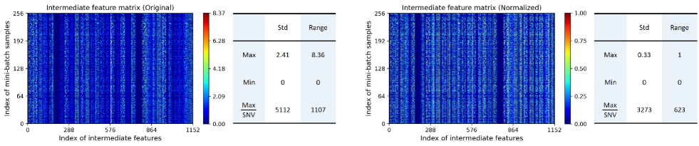
(a) IID

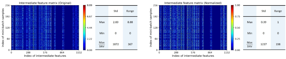
(b) non-IID

Figure 1: Visualization of original and normalized intermediate feature matrices for the MNIST dataset with $B=256$ and $\bar{D}=1,152$. The terms Std and SNV refer to the standard deviation and the smallest non-zero values, respectively.

• Forward propagation: Assume that device $k$ and the PS are engaged at iteration $t\in\{1,\ldots,T\}$, where $T$ is the total number of iterations. The parameter vectors of the device-side and server-side models are denoted by ${\bm{w}}_{\rm d}^{(t,k)}\in\mathbb{R}^{N_{\rm d}}$ and ${\bm{w}}_{\rm s}^{(t,k)}\in\mathbb{R}^{N_{\rm s}}$, respectively. A mini-batch for device $k$ at iteration $t$ is denoted by ${\bm{U}}^{(t,k)}=\{{\bm{u}}_{1}^{(t,k)},\ldots,{\bm{u}}_{B}^{(t,k)}\}$, where ${\bm{u}}_{i}^{(t,k)}\in\mathcal{D}_{k}$ and $B$ is the mini-batch size. The forward propagation process begins by transmitting the parameter vector of the device-side model ${\bm{w}}_{\rm d}^{(t,k)}$ from the PS or device $k-1$ to device $k$. Upon receiving this vector, device $k$ computes the intermediate feature matrix defined as

  $${\bm{F}}^{(t,k)}=g({\bm{w}}_{\rm d}^{(t,k)};{\bm{U}}^{(t,k)})\in\mathbb{R}^{B\times\bar{D}},$$ (3)

  where $\bar{D}$ is the dimension of intermediate features for one input data. Each column of ${\bm{F}}^{(t,k)}$ is denoted by ${\bm{f}}_{i}^{(t,k)},i\in\{1,\ldots,\bar{D}\}$ and each entry is denoted by $f_{b,i}^{(t,k)},b\in\{1,\ldots,B\}$. After computing the intermediate feature matrix in (3), device $k$ sends it along with the corresponding labels to the PS. Upon receiving ${\bm{F}}^{(t,k)}$ and the corresponding labels, the PS continues the forward propagation and then computes the mini-batch loss defined as

  $$h({\bm{w}}_{\rm s}^{(t,k)};{\bm{F}}^{(t,k)}) \triangleq\frac{1}{B}\sum_{i=1}^{B}f({\bm{w}}^{(t,k)};{\bm{u}}_{i}^{(t,k)}),$$ (4)

  where ${\bm{w}}^{(t,k)}=\big{[}({\bm{w}}_{\rm d}^{(t,k)})^{\sf T},({\bm{w}}_{\rm s}^{(t,k)})^{\sf T}\big{]}^{\sf T}$.

• Backward propagation: The backward propagation process begins by computing a gradient vector with respect to the server-side model, which is represented by ${\bm{g}}_{\rm s}^{(t,k)}=\nabla_{{\bm{w}}_{\rm s}}h({\bm{w}}_{\rm s}^{(t,k)};{\bm{F}}^{(t,k)})$. The PS then computes the intermediate gradient matrix defined as

  $${\bm{G}}^{(t,k)}=\nabla_{{\bm{F}}}h({\bm{w}}_{\rm s}^{(t,k)};{\bm{F}}^{(t,k)})\in\mathbb{R}^{B\times\bar{D}}.$$ (5)

  After computing the intermediate gradient matrix in (5), the PS transmits it to device $k$. Upon receiving ${\bm{G}}^{(t,k)}$, device $k$ proceeds with the backward propagation based on the chain rule. As a result, device $k$ obtains a gradient vector with respect to the device-side model, namely ${\bm{g}}_{\rm d}^{(t,k)}=\nabla_{{\bm{w}}_{\rm d}}h({\bm{w}}_{\rm s}^{(t,k)};{\bm{F}}^{(t,k)})$. Assuming that device $k$ and PS employ the SGD algorithm to update the parameter vectors of both device-side and server-side models, each parameter vector is updated as follows:

  $${\bm{w}}_{p}^{(t,k+1)} ={\bm{w}}_{p}^{(t,k)}-\eta{\bm{g}}_{p}^{(t,k)},~{}{p}\in\{{\rm d},{\rm s}\},$$ (6)

  where $\eta$ is the learning rate. After updating the parameters, the parameter vector of the device-side model is transmitted to the next device, and then the forward propagation process for that device is initiated. If the index $k$ reaches $K$, the forward propagation process for device $1$ is initiated, while the index $(t,K+1)$ is replaced with $(t+1,1)$. Meanwhile, if device $k$ and PS employ an alternative model updating algorithm, such as ADAM in [23], the gradient vector ${\bm{g}}_{\rm d}^{(t,k)}$ is transmitted from device $k$ to the PS, and then the PS updates both models.

II-B Key Challenge in SL

A key challenge in implementing the SL framework is the significant communication overhead necessary for transmitting the intermediate feature matrix in (3) from the device and the intermediate gradient matrix in (5) from the PS. This issue becomes increasingly problematic as the mini-batch size $B$ and the dimension $\bar{D}$ of intermediate feature for each input data grow. In order to make SL more practical, it is crucial to reduce the communication overhead for transmitting the intermediate feature matrix as well as the intermediate gradient matrix.

III Motivation and Overview

In this section, we present a novel communication-efficient SL framework designed to alleviate the communication overhead problem in SL. The proposed framework incorporates two adaptive feature-wise compression strategies: (i) adaptive feature-wise dropout and (ii) adaptive feature-wise quantization. We refer to this framework as SplitFC because it is a modified version of the original SL framework via feature-wise compression. In what follows, we first present the motivation behind developing two adaptive feature-wise compression strategies. Following that, we provide an overview of the SplitFC framework.

III-A Motivation

In a deep neural network, each intermediate layer can be thought of as a measurable feature, obtained by an output node of the device-side model from an attribute of the data sample [24]. As a result, some intermediate features may have similar values, indicating that the corresponding output nodes have captured common attributes in the mini-batch data samples. Conversely, some features may have significantly different values, suggesting that the corresponding output nodes have captured unique attributes. For example, consider SL for an image classification task using the MNIST dataset which consists of handwritten digit images. Certain output nodes of the device-side model may identify shared patterns such as loops or line segments common to multiple digits, leading to intermediate features with similar values. Other output nodes may distinguish between digits by recognizing unique attributes such as specific angles or intersections, resulting in intermediate features with dissimilar values. Consequently, intermediate features can exhibit varying levels of dispersion, which are typically measured by metrics such as standard deviation and range.

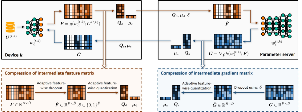
Figure 2: Illustration of the proposed SL framework with two adaptive feature-wise compression strategies.

To demonstrate the phenomenon described above, we present a simple numerical example in Fig. 1. This example involves an image classification task using the MNIST dataset, considering both independent and identically distributed (IID) and non-IID data distributions, with $T=100$. Further details of the simulation can be found in Sec. VI. In Fig. 1, we highlight the minimum, maximum, and ratio between the maximum and smallest non-zero values for both the standard deviation and range. The left-hand side of Fig. 1 shows that the intermediate feature vectors exhibit significant differences in their values, standard deviations, and ranges. Fig. 1 also shows that some intermediate vectors have almost no changes in their values. These results align with our hypothesis on the dispersion levels in the intermediate feature vectors. In the right-hand side (RHS) of Fig. 1, intermediate features are normalized to values between 0 and 1. Details of the normalization process will be elaborated in Sec. IV. The RHS of Fig. 1 provides additional insight into the issue of feature dispersion, showing that even after normalization, intermediate feature vectors still exhibit different ranges and standard deviations. However, the overall disparity of their values, standard deviations, and ranges across different intermediate feature vectors is significantly reduced. For instance, in the IID case, the original intermediate feature vectors with indices between $1,000$ and $1,050$ exhibit relatively low values. However, after normalization, these values become comparable to other large values. These results demonstrate the effectiveness of the normalization process in reducing the overall disparity of feature vectors and facilitating a fair comparison of their importance, as will be elaborated in Sec. IV.

III-B Overview of SplitFC

Motivated by the discussion in Sec. III-A, in SplitFC, we put forth the adaptive feature-wise dropout and quantization strategies for compressing the intermediate feature and gradient matrices, which leverage different dispersion degrees exhibited in the intermediate feature and gradient vectors. The high-level procedure of SplitFC is illustrated in Fig. 2 and summarized in Algorithm 1.

III-B1 Compression of the intermediate feature matrix

In each iteration, at each device, some of the intermediate feature vectors are probabilistically dropped using the adaptive feature-wise dropout strategy denoted by a function ${\sf FWDP}(\cdot)$. Following the dropout process, the remaining non-dropped intermediate feature vectors are quantized using the adaptive feature-wise quantization strategy denoted by a function ${\sf FWQ}(\cdot)$. Then, the compressed intermediate feature vectors, along with their corresponding indices, are transmitted to the PS. This compression procedure is summarized in lines 6 and 7 of Algorithm 1. Details on the adaptive feature-wise dropout strategy will be presented in Sec. IV.

III-B2 Compression of the intermediate gradient matrix

In each iteration, at the PS, the intermediate gradient matrix is computed based on the compressed intermediate feature matrix transmitted by each device. Then, by the chain rule, the intermediate gradient vectors corresponding to the indices of the dropped intermediate feature vectors are also dropped at the PS, while the remaining gradient vectors are quantized using the adaptive feature-wise quantization strategy. This compression procedure is summarized in lines 15 and 16 of Algorithm 1. Details on the adaptive feature-wise quantization strategy will be presented in Sec. V.

Algorithm 1 Communication-Efficient Split Learning via Adaptive Feature-Wise Compression (SplitFC)

1:Initial parameter vector ${\bm{w}}^{(1,1)}$, dimensionality reduction ratio $R$, communication overhead at the devices $C_{\rm e,d}$ (bits/entry), and communication overhead at the PS $C_{\rm e,s}$ (bits/entry)

2:Final parameter vector ${\bm{w}}^{(T,K)}$

3:for $t=1$ to $T$ do

4:   for $k=1$ to $K$ do

5:      $\bullet$ At the device $k$:

6:         Receive ${\bm{w}}_{\rm d}^{(t,k)}$ from device $(k-1)$ or the PS

7:         ${\bm{F}}=g({\bm{w}}_{\rm d}^{(t,k)};{\bm{U}}^{(t,k)})$

8:         $\tilde{\bm{F}},{\bm{\delta}}={\sf FWDP}\big{(}{\bm{F}},R\big{)}$ (Algorithm 2)

9:         ${\bm{Q}}_{\rm d},{\bm{\mu}}_{\rm d}={\sf FWQ}\big{(}\tilde{\bm{F}},C_{\rm e,d}\big{)}$ (Algorithm 3)

10:         Transmit ${\bm{Q}}_{\rm d}$, ${\bm{\mu}}_{\rm d}$, and ${\bm{\delta}}$ to the PS       

11:      $\bullet$ At the PS:

12:         Determine $\hat{\bm{F}}$ using ${\bm{Q}}_{\rm d}$, ${\bm{\mu}}_{\rm d}$, and ${\bm{\delta}}$

13:         Compute the mini-batch loss $h({\bm{w}}_{\rm s}^{(t,k)};\hat{\bm{F}})$

14:         Compute the gradient vector ${\bm{g}}_{\rm s}$ for ${\bm{w}}_{\rm s}^{(t,k)}$

15:         Update ${\bm{w}}_{\rm s}^{(t,k)}$ based on ${\bm{g}}_{\rm s}$

16:         ${\bm{G}}=\nabla_{\hat{\bm{F}}}h({\bm{w}}_{\rm s}^{(t,k)};\hat{\bm{F}})$

17:         Determine $\tilde{\bm{G}}$ by dropping $\{{\bm{g}}_{j}\}_{\forall j\notin\mathcal{I}}$

18:         ${\bm{Q}}_{\rm s},{\bm{\mu}}_{\rm s}={\sf FWQ}(\tilde{\bm{G}},C_{\rm e,s})$ (Algorithm 3)

19:         Transmit ${\bm{Q}}_{\rm s}$ and ${\bm{\mu}}_{\rm s}$ to device $k$       

20:      $\bullet$ At the device $k$:

21:         Determine $\hat{\bm{G}}$ using ${\bm{Q}}_{\rm s}$, ${\bm{\mu}}_{\rm s}$, and ${\bm{\delta}}$

22:         Compute the gradient vector ${\bm{g}}_{\rm d}$ for ${\bm{w}}_{\rm d}^{(t,k)}$

23:         Update ${\bm{w}}_{\rm d}^{(t,k)}$ based on ${\bm{g}}_{\rm d}$       

24:   end

25:end

IV Adaptive Feature-Wise Dropout Strategy

In this section, we present the adaptive feature-wise dropout strategy which aims at reducing the communication overhead required to transmit the intermediate feature and gradient matrices. The primary approach of this strategy is to probabilistically drop some of the intermediate feature vectors in order to reduce the size of the intermediate feature matrix prior to transmission. To ensure that important information within the intermediate feature matrix is preserved, feature vectors with high standard deviations are given priority and are less likely to be dropped. In the following, we provide the basic compression process of this strategy and then introduce the design of dropout probability for dropping intermediate feature vectors.

Algorithm 2 Adaptive Feature-Wise Dropout Strategy

1:Intermediate feature matrix ${\bm{F}}\in\mathbb{R}^{B\times\bar{D}}$ and dimensionality reduction ratio $R$

2:Compressed intermediate feature matrix $\tilde{\bm{F}}\in\mathbb{R}^{B\times\hat{D}}$ and index vector ${\bm{\delta}}$

3:procedure ${\sf FWDP}({\bm{F}},R)$

4:   $\displaystyle f_{\mathcal{I}_{h}}^{\rm max}=\max_{b\in\{1,\ldots,B\},i\in\mathcal{I}_{h}}f_{b,i},~{}f_{\mathcal{I}_{h}}^{\rm min}=\min_{b\in\{1,\ldots,B\},i\in\mathcal{I}_{h}}f_{b,i},$

5:   $\forall h\in\{1,\ldots,H\}$

6:   ${f}_{b,j}^{\rm norm}=({{f}_{b,j}-f_{\mathcal{I}_{h}}^{\rm min}})/({f_{\mathcal{I}_{h}}^{\rm max}-f_{\mathcal{I}_{h}}^{\rm min}}),$

7:   $\forall b\in\{1,\ldots,B\},\forall j\in\mathcal{I}_{h},\forall h$

8:   $\mu_{i}=\frac{1}{B}\sum_{b=1}^{B}f_{b,i}^{\rm norm},\forall i\in\{1,\ldots,\bar{D}\}$

9:   $\sigma_{i}=\big{\{}\frac{1}{B}\sum_{b=1}^{B}({f}_{b,i}^{\rm norm}-\mu_{i})^{2}\big{\}}^{1/2},\forall i$

10:   $D=\bar{D}/R$

11:   $q_{i}=({\sigma_{i}D})/({\sum_{j=1}^{\bar{D}}\sigma_{j}}),\forall i$

12:   $q^{\rm max}=\max_{i}q_{i}$

13:   $p_{i}=\begin{cases}1-q_{i},&q^{\rm max}\leq 1\\ 1-\frac{(\sigma_{i}+C)D}{\sum_{j=1}^{\bar{D}}(\sigma_{j}+C)},&q^{\rm max}>1\end{cases},\forall i$

14:   Generate the index vector ${\bm{\delta}}$ using $\{p_{i}\}_{\forall i}$

15:   $\hat{\bm{f}}_{i}={\delta_{i}}/({1-p_{i}}){\bm{f}}_{i},\forall i$

16:   $\mathcal{I}=\{i:\delta_{i}=1\}$

17:   Determine $\tilde{\bm{F}}$, with each column being $\hat{\bm{f}}_{j},j\in\mathcal{I}$

18:   return $\tilde{\bm{F}}$ and ${\bm{\delta}}$

19:end procedure

IV-A Basic Compression Process of Feature-Wise Dropout

In the proposed adaptive feature-wise dropout strategy, each intermediate feature vector ${\bm{f}}_{i},i\in\{1,\ldots,\bar{D}\}$ is dropped probabilistically with a dropout probability $p_{i}$ during training. Any non-dropped intermediate feature vectors are then scaled by a factor of $\frac{1}{1-p_{i}}$ to ensure that the expected value of the scaled feature vector remains the same as that of the original feature vector. The resulting intermediate feature vector of this strategy is denoted by $\hat{\bm{f}}_{i}$ and can be expressed as

$$\hat{\bm{f}}_{i}=\frac{\delta_{i}}{1-p_{i}}{\bm{f}}_{i},$$ (7)

where $\delta_{i}\in\{0,1\}$ is a Bernoulli random variable with $\mathbb{P}(\delta_{i}=1)=1-p_{i}$, indicating whether ${\bm{f}}_{i}$ is dropped or not. Let $\mathcal{I}=\{i:\delta_{i}=1\}$ be the index set of non-dropped feature vectors and $\bar{\bm{G}}=\nabla_{\hat{\bm{F}}}h({\bm{w}}_{\rm s};\hat{\bm{F}})\in\mathbb{R}^{B\times\bar{D}}$ be the intermediate gradient matrix computed at the PS. Then, based on the chain rule, the intermediate gradient vector that needs to be transmitted to the device can be expressed as

$$\hat{\bm{g}}_{j}=\begin{cases}\bar{\bm{g}}_{j},&j\in\mathcal{I},\\ {\bm{0}}_{B},&j\notin\mathcal{I}.\end{cases}$$ (8)

Let $\hat{D}=\sum_{i}\delta_{i}$ be the number of non-dropped feature vectors, $\tilde{\bm{F}}\in\mathbb{R}^{B\times\hat{D}}$ be the compressed intermediate feature matrix with each column being $\hat{\bm{f}}_{j},j\in\mathcal{I}$, and $\tilde{\bm{G}}\in\mathbb{R}^{B\times\hat{D}}$ be the compressed intermediate gradient matrix with each column being $\hat{\bm{g}}_{j},j\in\mathcal{I}$. Then, the equations in (7) and (8) show that the device only needs to transmit the compressed intermediate feature matrix $\tilde{\bm{F}}$, while the PS only needs to transmit the compressed intermediate gradient matrix $\tilde{\bm{G}}$, provided that the device and PS share the information of the index vector ${\bm{\delta}}$. Therefore, the feature-wise dropout strategy allows both the device and PS to achieve $\frac{\bar{D}}{\hat{D}}$ times reduction in the communication overhead for transmitting the intermediate feature and gradient matrices.

IV-B Design of Dropout Probability

To ensure that important features are preserved during the dropout process, we design the dropout probabilities by taking into account the standard deviations of the intermediate feature vectors. In our design, we prioritize intermediate feature vectors with high standard deviation to reduce the likelihood of dropping them. This prioritization is based on our assertion that intermediate feature vectors composed of dissimilar elements are likely to provide more valuable information for training the global model than those composed of similar elements. The rationale behind this assertion is that intermediate feature vectors composed of dissimilar elements contain unique attributes inherent in the training data and training the global model using these attributes can help to avoid overfitting to shared patterns in the training data, leading to better performance of the global model. In the following, we provide the details of our dropout probability design.

It is worth nothing that comparing the importance of feature vectors based solely on raw standard deviation may not be fair, as the range of feature values can vary significantly across different feature vectors (see Fig, 1(a)). To resolve this problem, we define a normalized feature as

$$\qquad\quad{f}_{b,j}^{\rm norm}=\frac{{f}_{b,j}-f_{\mathcal{I}_{h}}^{\rm min}}{f_{\mathcal{I}_{h}}^{\rm max}-f_{\mathcal{I}_{h}}^{\rm min}},$$

$$j\in\mathcal{I}_{h},b\in\{1,\ldots,B\},h\in\{1,\ldots,H\},$$ (9)

where $H$ represents the number of channels of the original intermediate feature map, $\mathcal{I}_{h}$ is the index set of feature vectors corresponding to $h$-th channel such that $\bigcup_{h=1}^{H}\mathcal{I}_{h}=\{1,\ldots,\bar{D}\}$ and $\mathcal{I}_{h_{1}}\cap\mathcal{I}_{h_{2}}=\emptyset,\forall h_{1}\neq h_{2}$. The minimum and maximum values among the feature vectors in the $h$-th channel are denoted by $f_{\mathcal{I}_{h}}^{\rm min}$ and $f_{\mathcal{I}_{h}}^{\rm max}$, respectively i.e., $f_{\mathcal{I}_{h}}^{\rm min}=\min_{b\in\{1,\ldots,B\},i\in\mathcal{I}_{h}}f_{b,i}$ and $f_{\mathcal{I}_{h}}^{\rm max}=\max_{b\in\{1,\ldots,B\},i\in\mathcal{I}_{h}}f_{b,i}$. The normalization step in (IV-B) ensures that each feature vector has values between 0 and 1 (see Fig. 1(b)), and allows a fair comparison of the importance of feature vectors. After the normalization, we compute the standard deviation of a normalized feature vector as follows:

$$\sigma_{i}=\sqrt{\frac{1}{B}\sum_{b=1}^{B}\left({f}_{b,i}^{\rm norm}-\mu_{i}\right)^{2}},$$ (10)

where $i\in\{1,\ldots,\bar{D}\}$ and $\mu_{i}=\frac{1}{B}\sum_{b=1}^{B}f_{b,i}^{\rm norm}$. Let $D$ be the average number of non-dropped feature vectors. Then, based on the standard deviation in (10), we define a constant $q_{i}$ as

$$q_{i}=\frac{\sigma_{i}D}{\sum_{j=1}^{\bar{D}}\sigma_{j}},$$ (11)

which quantifies the relative importance of the feature vector ${\bm{f}}_{i}$ compared to the others. We finally determine the dropout probability $p_{i}$ for the feature vector ${\bm{f}}_{i}$ as

$$p_{i}=\begin{cases}1-q_{i},&q^{\rm max}\leq 1,\\ 1-\frac{(\sigma_{i}+C_{\rm bias})D}{\sum_{j=1}^{\bar{D}}(\sigma_{j}+C_{\rm bias})},&q^{\rm max}>1,\end{cases}$$ (12)

where $q^{\rm max}=\max_{i\in\{1,\ldots,\bar{D}\}}q_{i}$, $\sigma^{\rm max}=\max_{i\in\{1,\ldots,\bar{D}\}}\sigma_{i}$ and $C_{\rm bias}\geq\frac{\sigma^{\rm max}D-\sum_{j}\sigma_{j}}{\bar{D}-D}$ is a hyper-parameter that serves as a bias to ensure that feature vectors with low standard deviation are selected while satisfying the probability axiom $0\leq p_{i}\leq 1$. The dropout probability in (12) shows that the larger the standard deviation, the smaller the dropout probability. This implies that intermediate feature vectors with high standard deviation are less likely to be dropped. From this principle, our adaptive feature-wise dropout strategy prioritizes feature vectors with higher standard deviations, ultimately reducing the likelihood of dropping important feature vectors. We summarize the overall procedure of this strategy in Algorithm 2.

Remark 1 (Average communication overhead of adaptive feature-wise dropout strategy): The expected value of $\hat{D}$ is determined as $\mathbb{E}[\hat{D}]=\mathbb{E}[\sum_{i}\delta_{i}]=\sum_{i}(1-p_{i})=D$. Therefore, the average communication overhead required by the device for transmitting the intermediate feature matrix in (7) is determined as

$$C_{\rm d}=\frac{32B\bar{D}}{R}+\bar{D},$$ (13)

where $R=\bar{D}/{D}>1$ is a dimensionality reduction ratio that controls the degree of compression and the second term on the RHS represents the communication overhead for transmitting the index vector ${\bm{\delta}}$. Similarly, the average communication overhead required by the PS for transmitting the intermediate gradient matrix in (8) is determined as

$$C_{\rm s}=\frac{32B\bar{D}}{R}.$$ (14)

The equations in (13) and (14) show that the dimensionality reduction ratio $R$ controls both uplink and downlink communication overheads.

Remark 2 (Comparison with traditional dropout): The traditional dropout strategy in [25, 26] is a widely-used regularization technique that generally involves randomly dropping individual features $\{f_{b,i}\}_{\forall b,i}$ according to certain dropout probabilities. In contrast, our adaptive feature-wise dropout strategy aims to reduce communication overhead in SL by probabilistically dropping individual feature vectors ${\bm{f}_{i}}$ with adaptive dropout probabilities. It is also noteworthy that our adaptive feature-wise dropout strategy can be applied to any model architecture, including dropout and pooling layers, making it more flexible and easier to incorporate into existing models. As such, this strategy can serve as a stand-alone technique or be used in conjunction with traditional dropout methods to further enhance model performance.

Algorithm 3 Adaptive Feature-Wise Quantization Strategy

1:Intermediate matrix ${\bm{A}}\in\mathbb{R}^{B\times\hat{D}}$ and communication overhead $C_{\rm e}$ (bits/entry)

2:$B\times M^{\star}$ matrix ${\bm{Q}}$, $(\hat{D}-M^{\star})$-dimensional vector ${\bm{\mu}}$

3:(Assuming that the intermediate feature vectors $\{{\bm{a}}_{i}\}_{i=1}^{\hat{D}}$ are sorted in descending order based on their range, without loss of generality)

4:procedure ${\sf FWQ}({\bm{A}},C_{\rm e})$

5:   $\displaystyle a_{i}^{\rm max}=\max_{b\in\{1,\ldots,B\}}a_{b,i},a_{i}^{\rm min}=\min_{b\in\{1,\ldots,B\}}a_{b,i},\forall i$

6:   $\bar{a}_{i}=\frac{1}{B}\sum_{b=1}^{B}a_{b,i},\forall i$

7:   Set $p^{\prime}$ to a large enough number

8:   for $n=1$ to $N$ do

9:      $M=M_{N-n+1}$

10:      $\displaystyle a^{\rm max}=\max_{j\in\{1,\ldots,M\}}a_{j}^{\rm max},a^{\rm min}=\max_{j\in\{1,\ldots,M\}}a_{j}^{\rm min}$

11:      $(\hat{a}_{u_{j}^{\rm min}},\hat{a}_{u_{j}^{\rm max}})={\sf Q}_{\rm ep}(a_{j}^{\rm min},a_{j}^{\rm max}),\forall j\in\{1,\ldots,M\}$

12:      $\displaystyle\bar{a}^{\rm max}=\max_{k\in\{M+1,\ldots,\hat{D}\}}\bar{a}_{k},~{}\bar{a}^{\rm min}=\min_{k\in\{M+1,\ldots,\hat{D}\}}\bar{a}_{k}$

13:      Solve the problem $({\bf P})$ and determine $\{\hat{Q}_{l}\}_{l=0}^{M}$

14:      $p=f(\hat{Q}_{0},\ldots,\hat{Q}_{M})$

15:      if $p>p^{\prime}$ then

16:         $\hat{Q}_{l}=\hat{Q}_{l}^{\prime},\forall l$, and $M^{\star}=M^{\prime}$

17:         break

18:      else if $n=N$ then

19:         $M^{\star}=M$

20:      else

21:         $\hat{Q}_{l}^{\prime}=\hat{Q}_{l},\forall l$, and $M^{\prime}=M$

22:      end

23:   end

24:   Quantize $\{{\bm{a}}_{j}\}_{j=1}^{M^{\star}}$ using the two-stage quantizer

25:   Quantize $\{\bar{a}_{k}\}_{k={M^{\star}+1}}^{\hat{D}}$ using the mean-value quantizer

26:   Determine ${\bm{Q}}$, with each column being ${\sf Q}_{j}({\bm{a}}_{j})$

27:   Determine ${\bm{\mu}}$, with each entry being ${\sf Q}_{0}(\bar{a}_{k})$

28:   return ${\bm{Q}}$ and ${\bm{\mu}}$

29:end procedure

V Adaptive Feature-Wise Quantization Strategy

The use of the adaptive feature-wise dropout strategy in Sec. IV effectively reduces the size of the intermediate feature and gradient matrices that need to be transmitted by each device and the PS, respectively. This size reduction alone, however, may not be sufficient for achieving a significant reduction in the communication overhead required for transmitting intermediate features and gradients. To further reduce the communication overhead in SL, in this section, we present the adaptive feature-wise quantization strategy which reduces the number of quantization bits for representing the compressed intermediate feature and gradient matrices, $\tilde{\bm{F}}$ and $\tilde{\bm{G}}$. For the sake of simplicity, in the remainder of this section, we will use the term “intermediate matrix” denoted by ${\bm{A}}\in\mathbb{R}^{B\times\hat{D}}$, which is a generic term for the aforementioned matrices. We will also use the term “intermediate vector” denoted by ${\bm{a}}_{i}\in\mathbb{R}^{B},i\in\{1,\ldots,\hat{D}\}$, representing $i$th column of ${\bm{A}}$. In addition, we shall assume that the intermediate vectors $\{{\bm{a}}_{i}\}_{i=1}^{\hat{D}}$ are sorted in descending order of the range without loss of generality.

V-A Quantizer Design

The fundamental idea of the adaptive feature-wise quantization strategy is to assign different quantization levels to intermediate vectors based on their ranges. Our key observation is that some intermediate vectors have almost no changes in their values, as can be seen in Fig. 1; thereby, quantizing the means of these vectors, instead of their entries, can effectively reduce the communication overhead even without significant quantization error. Motivated by this observation, we employ two types of quantizers: (i) a two-stage quantizer, and (ii) a mean-value quantizer. The two-stage quantizer is used for quantizing intermediate vectors with the $M$ largest ranges, while the mean-value quantizer is used for quantizing the mean of each of the remaining $\hat{D}-M$ vectors.

V-A1 Two-stage quantizer

Our two-stage quantizer, used for quantizing the intermediate vectors with the $M$ largest ranges, works as follows: In the first stage, the maximum and minimum values of the intermediate vector are quantized using an endpoint quantizer. This process helps determine the upper and lower limits of the vector’s entries using a lower bit budget. Then, in the second stage, the entries of the intermediate vector are quantized using an entry quantizer whose codebook is adpatively designed according the upper and lower limits determined by the endpoint quantizer. Let ${\sf Q}_{\rm ep}:\mathbb{R}^{2}\rightarrow\mathcal{C}_{\rm ep}^{2}$ be the endpoint quantizer which is common for the $M$ intermediate vectors, where $\mathcal{C}_{\rm ep}$ is the codebook of ${\sf Q}_{\rm ep}$ such that $|\mathcal{C}_{\rm ep}|=Q_{\rm ep}$, and $Q_{\rm ep}$ is the quantization level of ${\sf Q}_{\rm ep}$. To determine the endpoint quantizer, the maximum and minimum values of the entries of the $M$ intermediate vectors are computed as

$$a^{\rm max}=\min_{j\in\{1,\ldots,M\}}a_{j}^{\rm max}~{}\text{and}~{}a^{\rm min}=\min_{j\in\{1,\ldots,M\}}a_{j}^{\rm min},$$ (15)

respectively, where $a_{j}^{\rm max}=\max_{b\in\{1,\ldots,B\}}a_{b,j}$ and $a_{j}^{\rm min}=\min_{b\in\{1,\ldots,B\}}a_{b,j}$. Then, the $Q_{\rm ep}$-level uniform quantizer between $a^{\rm min}$ and $a^{\rm max}$ is employed as the endpoint quantizer, implying that $\mathcal{C}_{\rm ep}=\{\hat{a}_{1},\ldots,\hat{a}_{Q_{\rm ep}}\}$ with

$$\hat{a}_{u}=a^{\rm min}+(u-1)\Delta_{\rm ep},u\in\{1,\ldots,Q_{\rm ep}\},$$ (16)

and $\Delta_{\rm ep}=\frac{a^{\rm max}-a^{\rm min}}{Q_{\rm ep}-1}$. We assume that the quantization level $Q_{\rm ep}$ is shared by the PS and all the devices, while $a^{\rm min}$ and $a^{\rm max}$ are transmitted from the device to the PS. Under this assumption, the same codebook $\mathcal{C}_{\rm ep}$ can be generated at both the PS and the devices without explicitly exchanging the codebook itself. Utilizing the above quantizer, the maximum and minimum values of the $j$-th intermediate vector ${\bm{a}}_{j}$ are quantized as ${\sf Q}_{\rm ep}(a_{j}^{\rm min},a_{j}^{\rm max})=(\hat{a}_{u_{j}^{\rm min}},\hat{a}_{u_{j}^{\rm max}})$, where

$$u_{j}^{\rm min}=\left\lfloor\frac{a_{j}^{\rm min}-a^{\rm min}}{\Delta_{\rm ep}}\right\rfloor+1,~{}u_{j}^{\rm max}=\left\lceil\frac{a_{j}^{\rm max}-a^{\rm min}}{\Delta_{\rm ep}}\right\rceil+1,$$ (17)

for $j\in\{1,\ldots,M\}$. By the definition, the outputs of the endpoint quantizer, $\hat{a}_{u_{j}^{\rm max}}$ and $\hat{a}_{u_{j}^{\rm min}}$, correspond to the upper and lower limits of the entries in ${\bm{a}}_{j}$, respectively, i.e., $\hat{a}_{u_{j}^{\rm min}}\leq a_{b,j}\leq\hat{a}_{u_{j}^{\rm max}}$, $\forall b\in\{1,\ldots,B\}$. This implies that a proper range for quantizing the entries in ${\bm{a}}_{j}$ can be specified by using $2\log_{2}Q_{\rm ep}$ bits. Thanks to this feature, our endpoint quantization with $\log_{2}Q_{\rm ep}\ll 32$ requires a lower bit budget compared to explicitly transmitting the maximum and minimum values of ${\bm{a}}_{j}$. In the second stage, the entry quantizer for the $j$-th intermediate vector is determined by utilizing its upper and lower limits ($\hat{a}_{u_{j}^{\rm max}}$ and $\hat{a}_{u_{j}^{\rm min}}$) determined by the endpoint quantizer. Let ${\sf Q}_{j}:\mathbb{R}^{B}\rightarrow\mathcal{C}_{j}^{B}$ be the entry quantizer for the $j$-th intermediate vector for $j\in\{1,\ldots,M\}$, where $\mathcal{C}_{j}$ is the codebook of ${\sf Q}_{j}$ such that $|\mathcal{C}_{j}|=Q_{j}$, and $Q_{j}$ is the quantization level of ${\sf Q}_{j}$. The $Q_{j}$-level uniform quantizer between $\hat{a}_{u_{j}^{\rm min}}$ and $\hat{a}_{u_{j}^{\rm max}}$ is employed as the entry quantizer for ${\bm{a}}_{j}$, implying that $\mathcal{C}_{j}$ consists of $Q_{j}$ values that are equally spaced between $\hat{a}_{u_{j}^{\rm min}}$ and $\hat{a}_{u_{j}^{\rm max}}$. Then, the entries of the $j$-th intermediate vector are quantized using the quantizer ${\sf Q}_{j}$ for $j\in\{1,\ldots,M\}$. Let ${\bm{Q}}$ be a $B\times M$ matrix with each column being ${\sf Q}_{j}({\bm{a}}_{j})$. Then, the bit budget for transmitting ${\bm{Q}}$ is given by $B\sum_{j=1}^{M}\log_{2}Q_{j}$.

V-A2 Mean-value quantizer

Our mean-value quantizer, used for quantizing the means of the intermediate vectors with the $\hat{D}-M$ smallest ranges, is designed using a uniform quantizer. Let ${\sf Q}_{0}:\mathbb{R}\rightarrow{\mathcal{C}}_{0}$ be the mean-value quantizer which is common for the $\hat{D}-M$ intermediate vectors, where $\mathcal{C}_{0}$ is the codebook of ${\sf Q}_{0}$ such that $|\mathcal{C}_{0}|=Q_{0}$, and $Q_{0}$ is the quantization level of ${\sf Q}_{0}$. To determine the mean-value quantizer, the mean of each of the $\hat{D}-M$ intermediate vectors, denoted by $\bar{a}_{k}=\frac{1}{B}\sum_{b=1}^{B}a_{b,k}$, is computed for $k\in\{M+1,\ldots,\hat{D}\}$. Utilizing the computed means, the maximum and minimum mean values are computed as $\bar{a}^{\rm max}=\max_{k\in\{M+1,\ldots,\hat{D}\}}\bar{a}_{k}$ and $\bar{a}^{\rm min}=\min_{k\in\{M+1,\ldots,\hat{D}\}}\bar{a}_{k}$, respectively. We assume that $\bar{a}^{\rm min}$ and $\bar{a}^{\rm max}$ are transmitted from the device to the PS. Then, the $Q_{0}$-level uniform quantizer between $\bar{a}^{\rm min}$ and $\bar{a}^{\rm max}$ is employed as the mean-value quantizer, implying that ${\mathcal{C}}_{0}$ consists of $Q_{0}$ values that are equally spaced between $\bar{a}^{\rm min}$ and $\bar{a}^{\rm max}$. Utilizing this quantizer, the mean values in $\{\bar{a}_{k}\}_{k=M+1}^{\hat{D}}$ are quantized. Let ${\bm{\mu}}$ be a $(\hat{D}-M)$-dimensional vector with each entry being ${\sf Q}_{0}(\bar{a}_{k})$. Then, the bit budget for transmitting ${\bm{\mu}}$ is given by $(\hat{D}-M)\log_{2}Q_{0}$.

The total number of the quantization bits required by our adaptive feature-wise quantization strategy is given by

$$C_{\rm overhead}= ~{}2M\log_{2}Q_{\rm ep}+B\sum_{j=1}^{M}\log_{2}Q_{j}$$

$$+(\hat{D}-M)\log_{2}Q_{0}+\hat{D}+32\cdot 4.$$ (18)

In (18), the first and second term represent the total bit budget for the endpoint and entry quantization, respectively. The third term represents the bit budget for the mean-value quantization using the mean-value quantizer ${\sf Q}_{0}$. The fourth term represents the bit budget for indicating whether each intermediate vector is quantized by the two-stage quantizer or not. The fifth term represents the bit budget for explicitly transmitting $a^{\rm max}$, $a^{\rm min}$, $\bar{a}^{\rm max}$, and $\bar{a}^{\rm min}$ using floating-point representation.

One prominent feature of our strategy is the use of the mean value quantizer, which quantizes the mean of the intermediate vector instead of quantizing its entries independently. This quantizer can be an effective means of quantizing some intermediate vectors with almost no changes in their values, as can be seen from the numerical example in Fig. 1. Meanwhile, the mean value quantizer is dimension-free and therefore requires significantly fewer bits compared to an entry-wise quantizer. Another key feature of our strategy is the reduction of substantial bits required to determine a proper quantization range for each intermediate vector, by quantizing the maximum and minimum values of the vector using the endpoint quantizer. The quantization error of our strategy can be minimized by optimizing the quantization levels and the number $M$ of the intermediate vectors that need to be quantized using the two-stage quantizer, which will be discussed in the following subsections. The overall procedure of this strategy is summarized in Algorithm 3.

V-B Quantization Level Allocation

To minimize the quantization error of the proposed adaptive feature-wise quantization strategy, we optimize the quantization levels of the two-stage quantizers and the mean value quantizer. The quantization error of our strategy can be expressed as

$$\sum_{i=1}^{\hat{D}}\|{\bm{a}}_{i}-{\sf Q}_{i}({\bm{a}}_{i})\|^{2}=\sum_{i=1}^{{M}}{\sf QE}({\bm{a}}_{i},Q_{i})+\sum_{i=M+1}^{\hat{D}}{\sf QE}({\bm{a}}_{i},\bar{a}_{i}),$$ (19)

where ${\sf QE}({\bm{a}}_{i},Q_{i})=\|{\bm{a}}_{i}-{\sf Q}_{i}({\bm{a}}_{i})\|^{2}$, and ${\sf QE}({\bm{a}}_{i},\bar{a}_{i})=\|{\bm{a}}_{i}-{\sf Q}_{0}(\bar{a}_{i})\mathbbm{1}_{B}\|^{2}$. Considering the quantization of endpoints in the two-stage quantizer, the first term on the RHS of (19) is upper-bounded as

$${\sf QE}({\bm{a}}_{j},Q_{j})\overset{(a)}{\leq}\frac{\tilde{a}_{j}^{2}B}{4(Q_{j}-1)^{2}},$$ (20)

for all $j\in\{1,\ldots,M\}$, where $\tilde{a}_{j}=\hat{a}_{u_{j}^{\rm max}}-\hat{a}_{u_{j}^{\rm min}}$ and $(a)$ follows from the quantization error bound of uniform quantizer [27]. Considering the quantization of mean values in the mean-value quantizer, the second term on the RHS of (19) is upper-bounded as

$${\sf QE}({\bm{a}}_{k},\bar{a}_{k}) =\|{\bm{a}}_{k}-{\sf Q}_{0}(\bar{a}_{k})\mathbbm{1}_{B}\|^{2}$$

$$=\|{\bm{a}}_{k}-\bar{a}_{k}\mathbbm{1}_{B}+\bar{a}_{k}\mathbbm{1}_{B}-{\sf Q}_{0}(\bar{a}_{k})\mathbbm{1}_{B}\|^{2}$$

$$\leq 2\|{\bm{a}}_{k}-\bar{a}_{k}\mathbbm{1}_{B}\|^{2}+2\|\bar{a}_{k}\mathbbm{1}_{B}-{\sf Q}_{0}(\bar{a}_{k})\mathbbm{1}_{B}\|^{2}$$

$$\overset{(a)}{\leq}2\|{\bm{a}}_{k}-\bar{a}_{k}\mathbbm{1}_{B}\|^{2}+\frac{\tilde{a}_{0}^{2}B}{2(Q_{0}-1)^{2}},$$

$$\overset{(b)}{\leq}\frac{(a_{k}^{\rm max}-a_{k}^{\rm min})^{2}B}{2}+\frac{\tilde{a}_{0}^{2}B}{2(Q_{0}-1)^{2}},$$ (21)

for all $k\in\{M+1,\ldots,\hat{D}\}$, where $\tilde{a}_{0}=\bar{a}^{\rm max}-\bar{a}^{\rm min}$, $(a)$ follows from the quantization error bound of uniform quantizer [27] and $(b)$ follows from the result below.

$$\|{\bm{a}}_{k}-\bar{a}_{k}\mathbbm{1}_{B}\|^{2}$$

$$=\sum_{b=1}^{B}(a_{k,b}-a_{k}^{\rm min}+a_{k}^{\rm min}-\bar{a}_{k})^{2}$$

$$=\sum_{b=1}^{B}(a_{k,b}-a_{k}^{\rm min})^{2}-B(a_{k}^{\rm min}-\bar{a}_{k})^{2}$$

$$\overset{(a)}{\leq}(a_{k}^{\rm max}-a_{k}^{\rm min})\sum_{b=1}^{B}(a_{k,b}-a_{k}^{\rm min})-B(a_{k}^{\rm min}-\bar{a}_{k})^{2}$$

$$=B(\bar{a}_{k}-a_{k}^{\rm min})\{(a_{k}^{\rm max}-a_{k}^{\rm min})+(a_{k}^{\rm min}-\bar{a}_{k})\}$$

$$\overset{(b)}{\leq}\frac{(a_{k}^{\rm max}-a_{k}^{\rm min})^{2}B}{4},$$ (22)

where $(a)$ follows from $0\leq(a_{k,b}-a_{k}^{\rm min})\leq(a_{k}^{\rm max}-a_{k}^{\rm min})$ and $(b)$ follows from the arithmetic mean-geometric mean inequality.

Let $C_{\rm e}$ (bits/entry) be the maximum communication overhead (in terms of the bits per entry) allowed for transmitting $\tilde{\bm{F}}$ or $\tilde{\bm{G}}$. Then, the available bit budget for the adaptive feature-wise quantization strategy is given as follows:

1. If the device quantizes the compressed intermediate feature matrix $\tilde{\bm{F}}$, the index vector ${\bm{\delta}}\in\{0,1\}^{D}$ needs to be transmitted to the PS along with the quantized intermediate matrix. In this case, the available bit budget is given by

   $$C_{\rm ava}=B\bar{D}C_{\rm e}-\bar{D},$$ (23)

   where the second term on the RHS is the communication overhead for transmitting the index vector ${\bm{\delta}}$.

2. If the PS quantizes the compressed intermediate gradient matrix $\tilde{\bm{G}}$, the index vector ${\bm{\delta}}$ does not need to be transmitted. In this case, the available bit budget is given by

   $$C_{\rm ava}=B\bar{D}C_{\rm e}.$$ (24)

We then formulate the quantization level allocation problem given the available communication overhead $C_{\rm ava}$, by substituting the results in (20) and (V-B) into (19) as follows:

$$({\bf P})~{} \min_{\{Q_{i}\}_{i=0}^{M}}~{}\bigg{\{}f(Q_{0},\ldots,Q_{M})=\sum_{i=1}^{M}\frac{\tilde{a}_{i}^{2}B}{4(Q_{i}-1)^{2}}$$

$$\,\,\,\,+\sum_{i=M+1}^{\hat{D}}\frac{(a_{i}^{\rm max}-a_{i}^{\rm min})^{2}B}{2}+\frac{\tilde{a}_{0}^{2}B(\hat{D}-M)}{2(Q_{0}-1)^{2}}\bigg{\}},$$ (25)

$$~{}\text{s.t.}~{}1\leq\log_{2}Q_{l}\leq 32,\forall l\in\{0,\ldots,M\},$$ (26)

$$\quad\,\,\,\,C_{\rm overhead}\leq C_{\rm ava},$$ (27)

where the constraint in (26) specifies the maximum quantization level allowed for the entry quantizer for each intermediate vector. The problem $({\bf P})$ is a convex optimization problem and belongs to the family of water-filling problems, specifically cave-filling problems [28, 29]. Therefore, by utilizing the Karush-Kuhn-Tucker (KKT) conditions, we derive the optimal solution of the problem $({\bf P})$ as given in the following theorem:

Theorem 1:

The optimal solution of the problem $({\bf P})$ is

$$Q_{l}^{\star}=\min\left\{2^{32},\max\left\{2,\frac{(\frac{2}{3})^{\frac{1}{3}}u_{l}^{\star}}{v_{l}^{\star}}+\frac{v_{l}^{\star}}{2^{\frac{1}{3}}3^{\frac{2}{3}}}+1\right\}\right\},$$ (28)

for all $l\in\{0,\ldots,M\}$, where $u_{0}^{\star}=\frac{\tilde{a}_{0}^{2}B\log 2}{\nu^{\star}}$, $u_{j}^{\star}=\frac{\tilde{a}_{j}^{2}\log 2}{2\nu^{\star}},j\in\{1,\ldots,M\}$, $v_{l}^{\star}=(u_{l}^{\star}\sqrt{81-12u_{l}^{\star}}+9u_{l}^{\star})^{\frac{1}{3}},\forall l$, and $\nu^{\star}$ is the optimal Lagrange multiplier.

Proof:

See Appendix A. ∎

Theorem 1 demonstrates that the quantizer for an intermediate vector with a large range is allocated with a higher quantization level than that for an intermediate vector with a small range. This implies that the quantization level allocation in (28) naturally balances the quantization errors of intermediate vectors based on their ranges. Recall that the ranges of intermediate vectors can significantly differ as already discussed in Sec. III-A. Therefore, our quantization strategy with the optimal quantization level allocation effectively reduces the overall quantization error by adaptively quantizing the intermediate vectors according to their ranges.

The optimal Lagrange multiplier $\nu^{\star}$ in Theorem 1 can be easily obtained using various water-filling algorithms, such as the bisection search algorithm [29] and the fast water-filling algorithm [30]. Once $\nu^{\star}$ is acquired through any water-filling algorithm, the optimal quantization level is determined as shown in (28). However, in practical scalar quantizers, the quantization level is restricted to an integer value that is greater than or equal to two, denoted by $\hat{Q}_{l}$. As a result, the optimal solution in (28) might not be suitable for practical quantizers. One possible method to resolve this issue is to round down the solutions in (28) to consistently satisfy the bit budget constraint in (27) [31]. This approach has low computational complexity but may leave many unused bits. An alternative approach for better utilizing the available bit budget is to round off the solutions in (28) and then adjust the quantization levels based on $C_{\rm ava}$ and the differences denoted by $d_{j}=B(\log_{2}Q_{j}^{\star}-\log_{2}\hat{Q}_{j}),\forall j$ and $d_{0}=(\hat{D}-M)(\log_{2}Q_{0}^{\star}-\log_{2}\hat{Q}_{0})$ [32]. This technique satisfies the bit budget constraint in (27) while minimizing the number of unused bits.

The optimal quantization levels in Theorem 1 can be determined not only at the device, but also at the PS. This is because all the constants $\{\tilde{a}_{l}\}_{l=0}^{M}$ required for determining the optimal quantization levels can be computed at the PS using the information of $\bar{a}^{\rm max}$, $\bar{a}^{\rm min}$, and $\{\hat{a}_{u_{j}^{\rm min}},\hat{a}_{u_{j}^{\rm max}}\}_{j=1}^{M}$ which are already assumed to be transmitted from the device. Moreover, if the device explicitly transmits the optimal Lagrange multiplier $\nu^{\star}$, it is even not necessary to run the the water-filling algorithm at the PS. It is worth noting that the communication overhead required for transmitting a single constant $\nu^{\star}$ is negligible compared to the total communication overhead $C_{\rm overhead}$. These facts imply that both the device and the PS can generate the same optimal quantizers without explicitly exchanging the whole codebooks.

V-C Optimization of $M$

Utilizing the quantization error analysis and the optimal quantization levels presented in Sec. V-B, we also determine the best number $M^{\star}$ of the intermediate vectors that need to be quantized using the two-stage quantizer. To achieve this, we consider a pre-defined candidate set for $M$, given by $\mathcal{M}=\{M_{1},\ldots,M_{N}:0\leq M_{1}<\cdots<M_{N}\leq\hat{D}\}$. For each candidate $M\in\mathcal{M}$, we solve the problem $({\bf P})$, as described earlier, and evaluate the objective function in (V-B) using integer-valued quantization levels, i.e., $f(\hat{Q}_{0},\ldots,\hat{Q}_{M})$. We then determine the best number $M^{\star}$ by comparing the objective values and selecting the one that minimizes the objective function. To further reduce the computational complexity for determining $M^{\star}$, we can employ a stopping condition during the optimization process. For example, we can evaluate the objective values in descending order of $M$ and establish a stopping condition such that the evaluation halts if the current objective value is greater than the previous objective value. This method can save computation time, but still provides a reasonable estimate of $M^{\star}$. An outline of this method can be found in lines 12–21 of Algorithm 3.

VI Simulation Results and Analysis

In this section, we demonstrate the superiority of SplitFC over existing SL frameworks, using simulations. To account for communication overheads that occur during the training process, we define the uplink and downlink communication overheads required to transmit each entry of intermediate feature matrix ${\bm{F}}$ and intermediate gradient matrix ${\bm{G}}$ as $C_{\rm e,d}$ (bits/entry) and $C_{\rm e,s}$ (bits/entry), respectively. Our simulations are conducted for the image classification task using three publicly accessible datasets: MNIST [33], CIFAR-10 [34], and CelebA [35]. Details of the learning scenarios for each dataset are described below.

• MNIST: The global model is a simple variant of LeNet-5 in [33]. The device-side model includes an input layer, a $3\times 3$ convolutional layer with $16$ channels and one zero-padding, a $2\times 2$ max pooling layer with a stride size of $2$, a $3\times 3$ convolutional layer with $32$ channels, and a $2\times 2$ max pooling layer with a stride size of $2$. The server-side model comprises a fully connected layer with $1,152$ nodes, followed by another fully connected layer with $128$ nodes, and finally an output layer with softmax activation. The activation function used for the hidden layers in both models is the rectified linear unit. The device-side model contains $N_{\rm d}=4,800$ parameters, while the server-side model includes $N_{\rm s}=148,874$ parameters. To update both models, the ADAM optimizer in [23] is adopted with an initial learning rate of $0.001$. For the MNIST dataset, both IID and non-IID data distributions are considered. In the non-IID data distribution, data samples with the same label are divided into subsets, and each device is assigned only two subsets, each containing different labels [36]. In the simulations, the non-IID data distribution is considered unless otherwise specified, as it is a more realistic scenario in the context of SL [37]. The numbers of devices and communication rounds are set to be $K=30$ and $T=200$, respectively. The dimension of intermediate features for one input data is determined as $\bar{D}=1,152$, and the mini-batch size is set to be $B=256$.

• CIFAR-10: The global model is the VGG-16 network pre-trained on the ImageNet dataset [38], which comprises $40$ layers, and it is divided at the $20$th layer. The device-side model contains $N_{\rm d}=2,915,648$ parameters, while the server-side model includes $N_{\rm s}=131,385,866$ parameters. To update both models, the ADAM optimizer in [23] with an initial learning rate $0.0001$ is adopted. The data distribution is non-IID, determined by a Dirichlet distribution with a concentration parameter $\beta=0.3$ [36]. The numbers of devices and communication rounds are set to be $K=20$ and $T=200$, respectively. The dimension of intermediate features for one input data is determined as $\bar{D}=8,192$, and the mini-batch size is set to be $B=256$.

• CelebA: The global model is the MobileNetV3-Large network pre-trained on the ImageNet dataset [39], which comprises 192 layers, and it is divided at the $82$nd layer. The device-side model contains $N_{\rm d}=93,200$ parameters, while the server-side model includes $N_{\rm s}=4,111,394$ parameters. To update both models, the ADAM optimizer in [23] with an initial learning rate $0.0001$ is adopted. Each local training dataset is determined by randomly grouping $20$ writers in CelebA dataset [40]. The numbers of devices and communication rounds are set to be $K=100$ and $T=100$, respectively. The dimension of intermediate features for one input data is determined as $\bar{D}=13,440$, and the mini-batch size is set to be $B=64$.

For performance comparisons, we consider the following baselines:

• Vanilla SL: This framework assumes lossless transmission of the intermediate feature and gradient matrices with no compression, as described in Sec. II.

• SplitFC: This framework is the proposed SL framework summarized in Algorithm 1. In this framework, we set the hyper-parameter $C_{\rm bias}$ in (12) to $\frac{\sigma^{\rm max}D-\sum_{j}\sigma_{j}}{\bar{D}-D}$, the quantization level for endpoints to $Q_{\rm ep}=200$, and the candidate set as follows:

  $$\mathcal{M}=\left\{D^{\rm max}\cdot\frac{n}{10}:n\in\{1,\ldots,10\}\right\},$$ (29)

  where $D^{\rm max}=\min\big{(}\bar{D},\frac{C_{\rm ava}-2\hat{D}-32\cdot 4}{B+2\log_{2}Q_{\rm ep}-1}\big{)}$ represents the largest feasible value of $M$ for a specified bit budget $C_{\rm ava}$. Unless otherwise specified, we set the dimensionality reduction ratio $R$ to $16$.

• SplitFC-Rand: This framework is a simple modification of the adaptive feature-wise dropout strategy in the proposed SplitFC framework. In this framework, each intermediate feature vector ${\bm{f}}_{i}$ is randomly dropped with a dropout probability given by

  $$p_{i}=1-\frac{1}{R},\quad\forall i\in\{1,\ldots,\bar{D}\}.$$ (30)

• SplitFC-Deterministic: This framework is a simple modification of the adaptive feature-wise dropout strategy in the proposed SplitFC framework. In this framework, $(\bar{D}-D)$ intermediate feature vectors with small standard deviation in (10) are dropped.

• FedLite: This framework is the communication-efficient SL framework developed in [22]. In this framework, only the intermediate feature matrix is compressed, while the intermediate gradient matrix is transmitted with no compression. The number of groups is set to one, and the number of subvectors is carefully selected as a constant that yields the highest classification accuracy among the divisors of $\bar{D}$.

• Top-$S$: This framework is an extension of the communication-efficient federated learning framework in [21], with enhancements in performance and scalability. In this framework, the intermediate feature matrix is sparsified by retaining only the top-$S_{\rm d}$ entries with the largest magnitudes. The intermediate gradient matrix is sparsified using a similar technique to our SplitFC framework, where the intermediate gradient entries corresponding to the indices of the dropped intermediate feature entries are dropped. This is a key step for enhancing performance and reducing communication overhead. Additionally, if the downlink communication overhead is less than the uplink communication overhead, the remaining intermediate gradient entries are dropped by retaining only the top-$S_{\rm s}$ entries with the largest magnitudes. The sparsification levels $S_{\rm d}$ and $S_{\rm s}$ are determined as the largest integers $S_{1}$ and $S_{2}$ such that $32S_{1}+\log_{2}\big{(}\begin{smallmatrix}B\bar{D}\\ S_{1}\end{smallmatrix}\big{)}\leq B\bar{D}C_{\rm e,d}$ and $32S_{2}+\log_{2}\big{(}\begin{smallmatrix}S_{\rm d}\\ S_{2}\end{smallmatrix}\big{)}\leq B\bar{D}C_{\rm e,s}$, respectively.

In the simulations below, we compare the highest classification accuracies achieved by the considered SL frameworks within the same number of iterations $T$ to ensure a fair comparison.

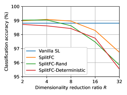
(a) IID

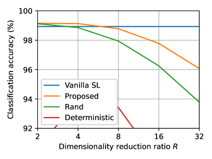
(b) non-IID

Figure 3: Classification accuracy of SplitFC-based frameworks for the MNIST dataset with different values of $R$.

In Fig. 3, we compare the classification accuracies of SplitFC-based frameworks, namely SplitFC, SplitFC-Rand, and SplitFC-Deterministic, for the MNIST dataset when the adaptive feature-wise quantization strategy is not applied. Fig. 3 demonstrates that SplitFC exhibits greater robustness against the decrease in the dimensionality reduction ratio $R$ compared to SplitFC-Rand and SplitFC-Deterministic. This result shows the limitations of randomly and deterministically dropping feature vectors, which do not consider the importance and fairness of individual intermediate feature vectors during the training process, respectively. Furthermore, this result supports our assertion that intermediate feature vectors containing dissimilar elements provide more valuable information for training the global model than those composed of similar elements, as discussed in Sec. IV-B. Meanwhile, SplitFC and SplitFC-Rand frameworks with low values of $R$ yield higher classification accuracy compared to the vanilla SL framework. This result suggests that the proposed adaptive feature-wise dropout strategy not only reduces the communication overhead but also has the potential to prevent neural networks from overfitting, as already reported in [25, 26].

TABLE I: Classification accuracy vs. uplink communication overhead for different SL frameworks.

Compression ratio		$1\times$	$80\times$	$160\times$	$320\times$
$C_{\rm e,d}$ (bits/entry)		$32$	$0.4$	$0.2$	$0.1$
MNIST	Vanilla SL	$98.93$	-	-	-
	SplitFC	-	${\bf 97.78}$	${\bf 97.77}$	${\bf 95.96}$
	FedLite	-	$94.73$	$85.25$	$70.19$
	Top-$S$	-	$89.62$	$79.05$	$78.28$
CIFAR-10	Vanilla SL	$86.88$	-	-	-
	SplitFC	-	${\bf 86.09}$	${\bf 85.98}$	${\bf 85.31}$
	FedLite	-	$85.04$	$80.57$	$75.56$
	Top-$S$	-	$83.16$	$82.01$	$79.71$
CelebA	Vanilla SL	$91.90$	-	-	-
	SplitFC	-	${\bf 92.23}$	${\bf 92.22}$	${\bf 91.84}$
	FedLite	-	$86.63$	$82.44$	$70.50$
	Top-$S$	-	$62.18$	$56.76$	$53.02$

In Table I, we compare the classification accuracies of various SL frameworks for the MNIST, CIFAR-10, and CelebA datasets. In these simulations, we apply only uplink compression while assuming lossless transmission of the intermediate gradient matrix for all baselines. Table I shows that the proposed SplitFC framework consistently achieves the highest classification accuracy, irrespective of the uplink communication overhead $C_{\rm e,d}$. In particular, the performance gap between SplitFC and the other baselines becomes more significant as the compression ratio increases. For instance, on the CelebA dataset, SplitFC achieves an accuracy of 97.84%, which is 21.34% higher than the second-best baseline, while they require 320 times less communication overhead compared to the vanilla SL framework. This result demonstrates the superiority of SplitFC and its robustness against the reduction in the uplink communication overhead.

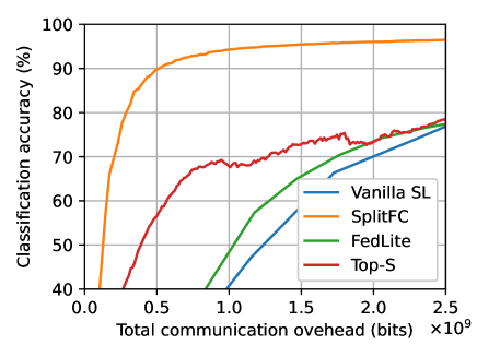
Figure 4: Classification accuracy vs. total communication overhead for different SL frameworks with the MNIST dataset.

In Fig. 4, we present a comprehensive evaluation of the classification accuracies achieved by various SL frameworks for the MNIST dataset. Our evaluation considers the total communication overhead of SL, computed as the sum of the communication costs required for transmitting parameters of device-side models at the PS, intermediate feature matrices at the devices, intermediate gradient matrices at the PS, and either parameters or gradients of device-side models at the devices. We assume that both the parameters and gradients of the device-side model are represented as 32-bit floating point values. Except for the vanilla SL framework, we set the uplink communication overhead as $C_{\rm e,d}=0.2$ bits/entry. Fig. 4 shows that the proposed SplitFC framework outperforms all baselines in terms of classification accuracy while maintaining a relatively low communication overhead. Specifically, SplitFC consistently exhibits a performance gap of over 15% compared to the other baselines across all levels of total communication overhead. Meanwhile, it is worth noting that the performance gap between SplitFC and other baselines can increase when the gradients of the device-side models are compressed using gradient compression techniques such as [8] and [41].

TABLE II: Classification accuracy vs. downlink communication overhead for different SL frameworks when the uplink communication overhead is $C_{\rm e,d}=0.4$ bits/entry.

Compression ratio		$1\times$	$40\times$	$80\times$	$160\times$
$C_{\rm e,s}$ (bits/entry)		$32$	$0.8$	$0.4$	$0.2$
MNIST	Vanilla SL	$98.93$	-	-	-
	$(C_{\rm e,d}=32)$
	SplitFC	-	$97.78$	${\bf 97.78}$	${\bf 97.74}$
	Top-$S$	-	-	$89.62$	$88.88$
CIFAR-10	Vanilla SL	$86.88$	-	-	-
	$(C_{\rm e,d}=32)$
	SplitFC	-	$86.06$	${\bf 85.99}$	${\bf 85.86}$
	Top-$S$	-	-	$83.23$	$83.18$
CelebA	Vanilla SL	$91.90$	-	-	-
	$(C_{\rm e,d}=32)$
	SplitFC	-	$92.23$	${\bf 92.21}$	${\bf 92.21}$
	Top-$S$	-	-	$62.18$	$61.81$

In Table II, we evaluate the classification accuracy of SplitFC for MNIST, CIFAR-10, and CelebA datasets when $C_{\rm e,d}=0.4$ bits/entry and $C_{\rm e,s}\in\{0.2,0.4,0.8\}$ bits/entry. Table II shows that the proposed SplitFC framework achieves the highest classification accuracy, consistently outperforming the Top-$S$ framework for all datasets. Moreover, Table II demonstrates that the classification accuracy of SplitFC does not degrade significantly even if the downlink communication overhead decreases. These results suggest that SplitFC effectively reduces the downlink communication overhead at the PS as well as the uplink communication overhead at the devices.

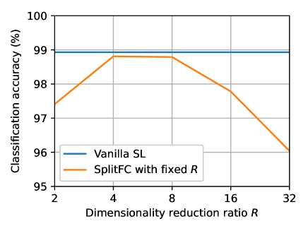
Figure 5: Classification accuracy of SplitFC for the MNIST dataset with various choices of $R$ when $C_{\rm e,d}=0.4$ bits/entry.

In Fig. 5, we evaluate the classification accuracy of SplitFC for the MNIST dataset by considering various choices of $R$. In this simulation, we assume lossless transmission of the intermediate gradient matrix and set the uplink communication overhead as $C_{\rm e,d}=0.4$ bits/entry. Fig. 5 shows that there exists an optimal selection of $R$ that yields the highest classification accuracy, even when the communication overhead remains constant (i.e., for a fixed $C_{\rm e,d}$). This phenomenon can be attributed to the fact that the performance of SplitFC relies on two types of errors: (i) dimensionality reduction error, and (ii) quantization error, both of which are determined by $R$. More specifically, as $R$ increases, the dimensionality reduction error also increases, resulting in performance degradation, as depicted in Fig. 3. Conversely, when $R$ increases, the quantization error decreases because the dimension of the intermediate matrix needed for quantization becomes smaller, even though the available bit-budget stays constant. For example, the performance with $R=16$ is shown to be worse than that with $R=8$ because of the dominant dimensionality reduction error. Although we have observed that there exists an optimal selection of $R$ that balances the trade-off between dimensionality reduction error and quantization error, deriving an analytic expression for this optimal $R$ remains an open problem, which is an important area for future work.

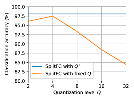
Figure 6: Classification accuracy of SplitFC with and without the quantization level optimization for the MNIST dataset with $C_{\rm e,d}=0.2$ bits/entry.

In Fig. 6, we compare the classification accuracy of SplitFC with and without the quantization level optimization discussed in Sec. V-B for the MNIST dataset. In this simulation, we assume lossless transmission of the intermediate gradient matrix and set the uplink communication overhead as $C_{\rm e,d}=0.2$ bits/entry. Without quantization level optimization, we set $Q_{l}=Q\in\{2,4,8,16,32\}$ for all $l\in\{0,\ldots,D_{Q}^{\rm max}\}$. Here, $D_{Q}^{\rm max}=\min\big{(}\bar{D},\frac{C_{\rm ava}-\hat{D}-32\cdot 4-\hat{D}\log_{2}Q}{B\log_{2}Q+2\log_{2}Q_{\rm ep}-\log_{2}Q}\big{)}$ is the largest feasible value of $M$ for a specified bit budget $C_{\rm ava}$ and a fixed quantization level $Q$. Fig. 6 shows that SplitFC with the quantization level optimization achieves a $13.6\%$ improvement in classification accuracy compared to SplitFC with the worst-case parameter (i.e., $Q=32$ case). This result demonstrates the effectiveness of our quantization level optimization in enhancing the overall performance of SplitFC.

VII Conclusion

In this paper, we have presented a communication-efficient SL framework that adaptively compresses intermediate feature and gradient matrices by exploiting various dispersion degrees exhibited in the columns of these matrices. In this framework, we have developed the adaptive feature-wise dropout and quantization strategies, which significantly reduce both uplink and downlink communication overheads in SL. Furthermore, we have minimized the quantization error of the presented framework by optimizing quantization levels allocated to different intermediate feature/gradient vectors. An important direction of future research is to extend the presented framework by considering the structure of intermediate features/gradients, such as channel-wise compression, to further enhance the SL performance under a limited communication overhead. Another promising research direction is to optimize the design of the dropout probabilities in the adaptive dropout strategy, by applying some advanced approaches, such as reinforcement learning.

Appendix A Proof of Theorem 1

The Lagrangian function for (V-B) is given by

$$\mathcal{L} (\{Q_{i}\}_{i=0}^{M},\nu,\lambda_{i},\gamma_{i})$$

$$= \sum_{i=1}^{M}\frac{\tilde{a}_{i}^{2}B}{4(Q_{i}-1)^{2}}+\sum_{i=M+1}^{\hat{D}}\frac{(a_{i}^{\rm max}-a_{i}^{\rm min})^{2}B}{2}$$

$$+\frac{\tilde{a}_{0}^{2}B(\hat{D}-M)}{2(Q_{0}-1)^{2}}$$

$$+\nu\bigg{\{}B\sum_{i=1}^{M}\log_{2}Q_{i}+(\hat{D}-M)\log_{2}Q_{0}+C_{\rm const}-C_{\rm ava}\bigg{\}}$$

$$+\sum_{i=0}^{M}\lambda_{i}(2-Q_{i})+\sum_{i=0}^{M}\gamma_{i}(Q_{i}-2^{32}),$$ (31)

where $C_{\rm const}=2M\log_{2}Q_{\rm ep}+\hat{D}+32\cdot 4$. Then, the KKT conditions for (A) are represented by

$$1\leq\log_{2}Q_{i}\leq 32,\forall i\in\{0,\ldots,M\},$$ (32)

$$\nu,\lambda_{i},\gamma_{i}\geq 0,\forall i,$$ (33)

$$\lambda_{i}(2-Q_{i})=0,\forall i,$$ (34)

$$\gamma_{i}(Q_{i}-2^{32})=0,\forall i,$$ (35)

$$\nu\bigg{\{}B\sum_{i=1}^{M}\log_{2}Q_{i}+(\hat{D}-M)\log_{2}Q_{0}+C_{\rm const}-C_{\rm ava}\bigg{\}}=0,$$ (36)

$$\frac{\nu B}{Q_{j}\log 2}-\frac{\tilde{a}_{j}^{2}B}{2(Q_{j}-1)^{3}}-\lambda_{j}+\gamma_{j}=0,\forall j\in\{1,\ldots,M\},$$ (37)

$$\frac{\nu(\hat{D}-M)}{Q_{0}\log 2}-\frac{\tilde{a}_{0}^{2}B(\hat{D}-M)}{(Q_{0}-1)^{3}}-\lambda_{0}+\gamma_{0}=0.$$ (38)

By multiplying (37) with $(2-Q_{j})$ and substituting (34) into the resulting expression, we obtain the following equation:

$$\bigg{(}\frac{\nu B}{Q_{j}\log 2}-\frac{\tilde{a}_{j}^{2}B}{2(Q_{j}-1)^{3}}+\gamma_{j}\bigg{)}(2-Q_{j})=0.$$ (39)

Under the condition in (32), two cases emerge from (39):

1. If ${Q_{j}}>2$, then the equation $\frac{\nu B}{Q_{j}\log 2}-\frac{\tilde{a}_{j}^{2}B}{2(Q_{j}-1)^{3}}+\gamma_{j}=0$ holds. Then, using the condition $\gamma_{j}\geq 0$ from (33), we can deduce that $\frac{\tilde{a}_{j}^{2}B}{2(Q_{j}-1)^{3}}-\frac{\nu B}{Q_{j}\log 2}\geq 0$. Solving this inequality with the consideration of $Q_{j}>2$, we obtain

   $$\nu<\tilde{a}_{j}^{2}\log 2,~{}\text{for}~{}Q_{j}>2.$$ (40)

2. If $Q_{j}=2$, then $\gamma_{j}=0$ from (35). Substituting this into (37) and using the condition $\lambda_{j}\geq 0$ from (33), we have

   $$\nu\geq\tilde{a}_{j}^{2}\log 2,~{}\text{for}~{}Q_{j}=2.$$ (41)

Next, multiplying (37) with $(Q_{j}-2^{32})$ and substituting (35) into the resulting expression, we have the following equation:

$$\bigg{(}\frac{\nu B}{Q_{j}\log 2}-\frac{\tilde{a}_{j}^{2}B}{2(Q_{j}-1)^{3}}-\lambda_{j}\bigg{)}(Q_{j}-2^{32})=0.$$ (42)

Under the condition in (32), two cases arise from (42):

1. If $Q_{j}<2^{32}$, then the equation $\frac{\nu B}{Q_{j}\log 2}-\frac{\tilde{a}_{j}^{2}B}{2(Q_{j}-1)^{3}}-\lambda_{j}=0$ holds. Then, using the condition $\lambda_{j}\geq 0$ from (33), we can derive that $\frac{\nu B}{Q_{j}\log 2}-\frac{\tilde{a}_{j}^{2}B}{2(Q_{j}-1)^{3}}\geq 0$. Solving this inequality with the consideration of $Q_{j}<2^{32}$, we have

   $$\nu>\frac{2^{31}\tilde{a}_{j}^{2}\log 2}{(2^{32}-1)^{3}},~{}\text{for}~{}Q_{j}<2^{32}.$$ (43)

2. If $Q_{j}=2^{32}$, then $\lambda_{j}=0$ from (34). Substituting this into (37) and using the condition $\gamma_{j}\geq 0$ from (33), we have

   $$\nu\leq\frac{2^{31}\tilde{a}_{j}^{2}\log 2}{(2^{32}-1)^{3}},~{}\text{for}~{}Q_{j}=2^{32}.$$ (44)

Next, consider the case $2<Q_{j}<2^{32}$. In this case, both $\lambda_{j}$ and $\gamma_{j}$ are equal to 0 according to conditions (34) and (35), respectively. Substituting these values into the condition in (37), we obtain the following equation:

$$(Q_{j}-1)^{3}=\frac{\tilde{a}_{j}^{2}\log 2}{2\nu}Q_{j},~{}\text{for}~{}2<Q_{j}<2^{32}.$$ (45)

Given the results in (40) and (43), we know that $\frac{1}{2}<\frac{\tilde{a}_{j}^{2}\log 2}{2\nu}<\frac{(2^{32}-1)^{3}}{2^{32}}$. Utilizing this inequality, we can derive the unique solution for (45) as follows:

$$Q_{j}=\frac{(\frac{2}{3})^{\frac{1}{3}}u_{j}}{v_{j}}+\frac{v_{j}}{2^{\frac{1}{3}}3^{\frac{2}{3}}}+1,~{}\text{for}~{}2<Q_{j}<2^{32},$$ (46)

where $u_{j}=\frac{\tilde{a}_{j}^{2}\log 2}{2\nu}$ and $v_{j}=(u_{j}\sqrt{81-12u_{j}}+9u_{j})^{\frac{1}{3}}$. Finally, combining the results in (41), (44), and (46), we obtain

$$Q_{j}=\begin{cases}2,&\nu\geq\tilde{a}_{j}^{2}\log 2,\\ \frac{(\frac{2}{3})^{\frac{1}{3}}u_{j}}{v_{j}}+\frac{v_{j}}{2^{\frac{1}{3}}3^{\frac{2}{3}}}+1,&\frac{2^{31}\tilde{a}_{j}^{2}\log 2}{(2^{32}-1)^{3}}<\nu<\tilde{a}_{j}^{2}\log 2,\\ 2^{32},&\nu\leq\frac{2^{31}\tilde{a}_{j}^{2}\log 2}{(2^{32}-1)^{3}}.\end{cases}$$ (47)

Similarly, we can determine the value of $Q_{0}$ using a procedure analogous to the one described above. Specifically, $Q_{0}$ is obtained as follows:

$$Q_{0}=\begin{cases}2,&\nu\geq\tilde{a}_{0}^{2}B\log 4,\\ \frac{(\frac{2}{3})^{\frac{1}{3}}u_{0}}{v_{0}}+\frac{v_{0}}{2^{\frac{1}{3}}3^{\frac{2}{3}}}+1,&\frac{2^{32}\tilde{a}_{0}^{2}B\log 2}{(2^{32}-1)^{3}}<\nu<\tilde{a}_{0}^{2}B\log 4,\\ 2^{32},&\nu\leq\frac{2^{32}\tilde{a}_{0}^{2}\log 2}{(2^{32}-1)^{3}},\end{cases}$$ (48)

where $u_{0}=\frac{\tilde{a}_{0}^{2}B\log 2}{\nu}$ and $v_{0}=(u_{0}\sqrt{81-12u_{0}}+9u_{0})^{\frac{1}{3}}$. The Lagrange multiplier $\nu$ must fulfill the condition in (36), and the optimal Lagrange multiplier $\nu^{\star}$ can be obtained using a variety of water-filling algorithms found in the literature [29, 30]. Once $\nu^{\star}$ is obtained, the optimal quantization level can be determined as shown in (28) of Theorem 1.

References

- [1] J. Konečnỳ, B. McMahan, and D. Ramage, “Federated optimization: Distributed optimization beyond the datacenter,” in Proc. Neural Inf. Process. Syst. (NIPS) Workshop Optim. Mach. Learn., Montreal, QC, Canada, Dec. 2015, pp. 1–5.
- [2] B. McMahan, E. Moore, D. Ramage, S. Hampson, and B. A. y. Arcas, “Communication-efficient learning of deep networks from decentralized data,” in Proc. Int. Conf. Artificial Intell. Statist. (AISTATS), vol. 54, Fort Lauderdale, FL, USA, Apr. 2017, pp. 1273–1282.
- [3] S. Niknam, H. S. Dhillon, and J. H. Reed, “Federated learning for wireless communications: Motivation, opportunities, and challenges,” IEEE Commun. Mag., vol. 58, no. 6, pp. 46–51, Jun. 2020.
- [4] Y.-S. Jeon, M. M. Amiri, J. Li, and H. V. Poor, “A compressive sensing approach for federated learning over massive MIMO communication systems,” IEEE Trans. Wireless Commun., vol. 20, no. 3, pp. 1990–2004, Mar. 2021.
- [5] F. Sattler, S. Wiedemann, K.-R. Müller, and W. Samek, “Robust and communication-efficient federated learning from non-iid data,” IEEE Trans. Neural Netw. Learn. Syst., vol. 31, no. 9, pp. 3400–3413, Sep. 2020.
- [6] M. Chen, Z. Yang, W. Saad, C. Yin, H. V. Poor, and S. Cui, “A joint learning and communications framework for federated learning over wireless networks,” IEEE Trans. Wireless Commun., vol. 20, no. 1, pp. 269–283, Jan. 2021.
- [7] G. Zhu, D. Liu, Y. Du, C. You, J. Zhang, and K. Huang, “Toward an intelligent edge: Wireless communication meets machine learning,” IEEE Commun. Mag., vol. 58, no. 1, pp. 19–25, May 2020.
- [8] Y. Oh, N. Lee, Y.-S. Jeon, and H. V. Poor, “Communication-efficient federated learning via quantized compressed sensing,” IEEE Trans. Wireless Commun., vol. 22, no. 2, pp. 1087–1100, Feb. 2023.
- [9] Y. Oh, Y.-S. Jeon, M. Chen, and W. Saad, “FedVQCS: Federated learning via vector quantized compressed sensing,” 2022, arXiv:2204.07692.
- [10] C. Thapa, P. C. M. Arachchige, S. Camtepe, and L. Sun, “SplitFed: When federated learning meets split learning,” in Proc. AAAI Conf. Artif. Intell., Jun. 2022, pp. 8485–8493.
- [11] T. Guo, S. Guo, F. Wu, W. Xu, J. Zhang, Q. Zhou, Q. Chen, and W. Zhuang, “Tree learning: Towards promoting coordination in scalable multi-client training acceleration,” IEEE Trans. Mobile Comput., early access, Mar. 20, 2023, doi: 10.1109/TMC.2023.3259007.
- [12] T. Li, A. K. Sahu, A. Talwalkar, and V. Smith, “Federated learning: Challenges, methods, and future directions,” IEEE Signal Process. Mag., vol. 37, no. 3, pp. 50–60, May 2020.
- [13] D.-J. Han, D.-Y. Kim, M. Choi, C. G. Brinton, and J. Moon, “SplitGP: Achieving both generalization and personalization in federated learning,” in Proc. IEEE Int. Conf. Comput. Commun. (INFOCOM), New York, NY, USA, May 2023.
- [14] O. Gupta and R. Raskar, “Distributed learning of deep neural network over multiple agents,” J. Netw. Comput. Appl., vol. 116, pp. 1–8, Aug. 2018.
- [15] P. Vepakomma, O. Gupta, T. Swedish, and R. Raskar, “Split learning for health: Distributed deep learning without sharing raw patient data,” in Proc. Int. Conf. Learn. Represent. (ICLR) Workshop AI Social Good, New Orleans, LA, USA, May 2019, pp. 1–7.
- [16] K. B. Letaief, Y. Shi, J. Lu, and J. Lu, “Edge artificial intelligence for 6g: Vision, enabling technologies, and applications,” IEEE J. Sel. Areas Commun., vol. 40, no. 1, pp. 5–36, Jan. 2022.
- [17] N.-P. Tran, N.-N. Dao, T.-V. Nguyen, and S. Cho, “Privacy-preserving learning models for communication: A tutorial on advanced split learning,” in Int. Conf. Inf. Commun. Technol. Convergence (ICTC), Jeju Island, Republic of Korea, Oct. 2022, pp. 1059–1064.
- [18] X. Chen, J. Li, and C. Chakrabarti, “Communication and computation reduction for split learning using asynchronous training,” in Proc. IEEE Workshop Signal Process. Syst. (SiPS), Coimbra, Portugal, Oct. 2021, pp. 76–81.
- [19] D.-J. Han, H. I. Bhatti, J. Lee, and J. Moon, “Accelerating federated learning with split learning on locally generated losses,” in Proc. Int. Conf. Mach. Learn. (ICML) Workshop Federated Learn. User Privacy Data Confidentiality, Jul. 2021.
- [20] A. Ayad, M. Renner, and A. Schmeink, “Improving the communication and computation efficiency of split learning for IoT applications,” in Proc. IEEE Glob. Commun. Conf. (GLOBECOM), Madrid, Spain, Dec. 2021, pp. 1–6.
- [21] B. Yuan, S. Ge, and W. Xing, “A federated learning framework for healthcare IoT devices,” 2020, arXiv:2005.05083.
- [22] J. Wang, H. Qi, A. S. Rawat, S. Reddi, S. Waghmare, F. X. Yu, and G. Joshi, “FedLite: A scalable approach for federated learning on resource-constrained clients,” 2022, arXiv:2201.11865.
- [23] D. P. Kingma and J. Ba, “Adam: A method for stochastic optimization,” in Proc. Int. Conf. Learn. Represent. (ICLR), San Diego, CA, USA, May 2015, pp. 1–13.
- [24] Y. LeCun, Y. Bengio, and G. Hinton, “Deep learning,” Nature, vol. 521, no. 7553, pp. 436–444, May 2015.
- [25] G. E. Hinton, N. Srivastava, A. Krizhevsky, I. Sutskever, and R. R. Salakhutdinov, “Improving neural networks by preventing co-adaptation of feature detectors,” 2012, arXiv:1207.0580.
- [26] N. Srivastava, G. Hinton, A. Krizhevsky, I. Sutskever, and R. Salakhutdinov, “Dropout: A simple way to prevent neural networks from overfitting,” J. Mach. Learn. Res., vol. 15, no. 56, pp. 1929–1958, Jun. 2014.
- [27] S. K. Mitra, Digital signal processing: A computer-based approach. New York, NY, USA: McGraw-Hill, 2001.
- [28] F. Gao, T. Cui, and A. Nallanathan, “Optimal training design for channel estimation in decode-and-forward relay networks with individual and total power constraints,” IEEE Trans. Signal Process., vol. 56, no. 12, pp. 5937–5949, Dec. 2008.
- [29] L. Zhang, Y. Xin, Y.-C. Liang, and H. V. Poor, “Cognitive multiple access channels: Optimal power allocation for weighted sum rate maximization,” IEEE Trans. Commun., vol. 57, no. 9, pp. 2754–2762, Sep. 2009.
- [30] X. Ling, B. Wu, P.-H. Ho, F. Luo, and L. Pan, “Fast water-filling for agile power allocation in multi-channel wireless communications,” IEEE Commun. Lett., vol. 16, no. 8, pp. 1212–1215, Aug. 2012.
- [31] Y. Du, S. Yang, and K. Huang, “High-dimensional stochastic gradient quantization for communication-efficient edge learning,” IEEE Trans. Signal Process., vol. 68, pp. 2128–2142, Mar. 2020.
- [32] P. S. Chow, J. M. Cioffi, and J. A. C. Bingham, “A practical discrete multitone transceiver loading algorithm for data transmission over spectrally shaped channels,” IEEE Trans. Commun., vol. 43, no. 2/3/4, pp. 773–775, Feb./Mar./Apr. 1995.
- [33] Y. Lecun, L. Bottou, Y. Bengio, and P. Haffner, “Gradient-based learning applied to document recognition,” Proc. IEEE, vol. 86, no. 11, pp. 2278–2324, Nov. 1998.
- [34] A. Krizhevsky, “Learning multiple layers of features from tiny images,” M.S. thesis, Univ. Toronto, Toronto, ON, Canada, 2009.
- [35] S. Caldas, S. M. K. Duddu, P. Wu, T. Li, J. Konečnỳ, H. B. McMahan, V. Smith, and A. Talwalkar, “Leaf: A benchmark for federated settings,” in Proc. Neural Inf. Process. Syst. (NIPS), Vancouver, BC, Canada, Dec. 2019, pp. 1–14.
- [36] Q. Li, Y. Diao, Q. Chen, and B. He, “Federated learning on non-iid data silos: An experimental study,” in IEEE Int. Conf. Data Eng. (ICDE), Kuala Lumpur, Malaysia, May 2022, pp. 965–978.
- [37] Y. Gao, M. Kim, S. Abuadbba, Y. Kim, C. Thapa, K. Kim, S. A. Camtep, H. Kim, and S. Nepal, “End-to-end evaluation of federated learning and split learning for internet of things,” in Int. Symp. Reliable Distrib. Syst. (SRDS), Shanghai, China, Sep. 2020, pp. 91–100.
- [38] K. Simonyan and A. Zisserman, “Very deep convolutional networks for large-scale image recognition,” in Proc. Int. Conf. Learn. Represent. (ICLR), San Diego, CA, USA, May 2015, pp. 1–14.
- [39] A. Howard, M. Sandler, G. Chu, L.-C. Chen, B. Chen, M. Tan, W. Wang, Y. Zhu, R. Pang, V. Vasudevan, Q. V. Le, and H. Adam, “Searching for MobileNetV3,” in Proc. IEEE/CVF Int. Conf. Comput. Vis. (ICCV), Oct. 2019, pp. 1314–1324.
- [40] Y. Jiang, S. Wang, V. Valls, B. J. Ko, W.-H. Lee, K. K. Leung, and L. Tassiulas, “Model pruning enables efficient federated learning on edge devices,” IEEE Trans. Neural Netw. Learn. Syst., early access, Apr. 25, 2022, doi: 10.1109/TNNLS.2022.3166101.
- [41] J. Bernstein, Y.-X. Wang, K. Azizzadenesheli, and A. Anandkumar, “SignSGD: Compressed optimisation for non-convex problems,” in Proc. Int. Conf. Mach. Learn. (ICML), Stockholmsmässan, Stockholm Sweden, Jul. 2018, pp. 560–569.