Spatial-Temporal Data Mining for Ocean Science: Data, Methodologies and Opportunities

Abstract.

With the rapid amassing of spatial-temporal (ST) ocean data, many spatial-temporal data mining (STDM) studies have been conducted to address various oceanic issues, including climate forecasting and disaster warning. Compared with typical ST data (e.g., traffic data), ST ocean data is more complicated but with unique characteristics, e.g., diverse regionality and high sparsity. These characteristics make it difficult to design and train STDM models on ST ocean data. To the best of our knowledge, a comprehensive survey of existing studies remains missing in the literature, which hinders not only computer scientists from identifying the research issues in ocean data mining but also ocean scientists to apply advanced STDM techniques. In this paper, we provide a comprehensive survey of existing STDM studies for ocean science. Concretely, we first review the widely-used ST ocean datasets and highlight their unique characteristics. Then, typical ST ocean data quality enhancement techniques are explored. Next, we classify existing STDM studies in ocean science into four types of tasks, i.e., prediction, event detection, pattern mining, and anomaly detection, and elaborate on the techniques for these tasks. Finally, promising research opportunities are discussed. This survey can help scientists from both computer science and ocean science better understand the fundamental concepts, key techniques, and open challenges of STDM for ocean science.

1. Introduction

Ocean, covering more than two-thirds of the earth, plays an important role in various applications (e.g., climate forecasting and ocean transportation (Lou et al., 2023)), and is critical to human survival and sustainable development. Many real-world events and phenomena (e.g., El Ni$\mathrm{\tilde{n}}$o, typhoons and ocean currents) occurring in ocean generally not only are associated with spatial locations but also change over time. Thus, the collected ocean data for monitoring these events and phenomena are typically spatial-temporal (ST) data in nature and require specific spatial-temporal data mining (STDM) techniques to conduct data analysis. As shown in Fig. 2, STDM for ocean science aims to uncover the ST patterns and correlations from various ST ocean data, helps us better understand the ocean system, and provides valuable support for various real-world applications. For example, accurate prediction of sea surface temperature (SST) is of great significance in weather forecasting, El Ni$\mathrm{\tilde{n}}$o event detection, and disaster warning, and could also benefit aquaculture and agriculture (Aguilar-Martinez and Hsieh, 2009).

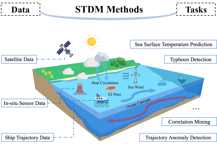
Figure 1. The illustration of STDM for ocean science, which utilizes various STDM methods to discover unknown but potentially useful patterns from different ocean data sources for a number of data mining tasks.

Figure 2. 1980-2022 publications of STDM studies for ocean science (Results from Web of Science with query keywords: [Spatial temporal & ocean] or [Spatio-temporal & ocean]).

The past decades have witnessed ever-increasing ST ocean data and lots of research on STDM for ocean science, which lays the solid foundation for addressing various oceanic issues in the data-driven paradigm. With the rapid development of data sensing technologies, numerous ocean observation sensors of different types have been deployed on various platforms including space remote satellites, automatic buoys, and vessels all over the world, producing large amounts of ST data of ocean. To be more specific, an estimate puts the size of ST ocean data in 2030 at 350 Petabytes (1 PB = 1,000 TB), and this number is predicted to grow exponentially (Overpeck et al., 2011). With such huge amounts of ST ocean data, an increasing number of studies on STDM for ocean science have been conducted. According to incomplete statistics of the related publications from 1980 to 2022 on Web of Science, as shown in Fig. 2, ocean STDM receives increasing attention over time and the increasing trend in the last three years is especially obvious. This trend indicates that STDM for ocean science has become a hot research topic in recent years.

Though STDM for ocean science is a vibrant interdisciplinary field, there are still some obstacles that hinder its development and applications.

First, there is a lack of review on available ST ocean datasets and their unique data characteristics. In the past decades, ST ocean datasets collected from different sources have been released by various producers, e.g., National Oceanic and Atmospheric Administration (NOAA), National Aeronautics and Space Administration (NASA), and European Centre for Medium-Range Weather Forecasts (ECMWF). However, these datasets have diverse data collection protocols, sensors, and technologies, leading to diversity in data resolution, coverage, and quality. Currently, there is no systematic review of these data to facilitate researchers to choose appropriate datasets for studying different problems and tasks of ocean science. Moreover, ST ocean data has some unique characteristics, e.g., diverse regionality, high sparsity, inherent uncertainty, and deep ST dependencies, which are also not well investigated. For example, due to the large-scale coverage of the ocean on Earth, there exists diverse regionality in different areas. The collected ST ocean data in the Arctic Ocean may have opposite seasonality patterns from the data near the equator, which is difficult to model in a unified system. According to (Lian et al., 2023), the extreme weather in remote regions (e.g., the Antarctica Ocean) makes it difficult to deploy the in-situ sensors to collect data, and the heavy cloud in some periods may cause more than 80% of satellite data to be lost, which are two main reasons for the data sparsity problem. The sensors’ stability and transmission loss may both cause uncertainty in ocean data. In addition, the complex and unknown ocean circulation as well as teleconnection between different regions in the ocean (Li et al., 2021a) may bring deep and hidden ST dependencies in the data. Ignoring these unique data characteristics could lead to low accuracy and bad interpretability of the STDM methods for ocean science. Therefore, from the data perspective, it is necessary to analyze the widely-used ST ocean datasets and identify their unique data characteristics.

Table 1. A summary of the related surveys on STDM.

Year	Ref.	Contribution	Scope
			Data	Data Quality	Tasks & Methodologies
					ST Prediction	Event Detection	Pattern Mining	Anomaly Detection
2014	(Faghmous and Kumar, 2014)	Overview the STDM methods and give some case studies of climate data.			✓	✓	✓
2015	(Shekhar et al., 2015)	Provide a complexity comparison of typical STDM methods.				✓	✓
2019	(Wang et al., 2022a)	Summarize the latest deep learning methods in STDM.			✓		✓	✓
2020	(Kim et al., 2020)	Overview the GAN-based models for ST data completion.		✓
2021	(Haghbin et al., 2021)	Overview the ST methods for SST prediction.	✓		✓
2022	(Wu et al., 2022)	Summarize the current research methodologies and the challenges of STDM in ocean domain.	✓		✓	✓		✓
2022	(Sharma et al., 2022)	Overview of the latest STDM methods for mutilple fieids.			✓	✓	✓
2022	(Hamdi et al., 2022)	Summarize some challenging issues and open problems of multiple STDM directions.			✓		✓	✓
Ours		A survey of STDM methods for ocean science: multi-source datasets with unique characteristics, data quality enhancement methods, advanced models in various tasks, and future directions.	✓	✓	✓	✓	✓	✓

Second, although there are already some surveys on STDM in the literature, we do not see any systematic and comprehensive surveys on STDM techniques for ocean science. Table 1 summarizes and compares the related surveys of STDM in terms of contribution and scope. To provide a clear comparison, we put different oceanic STDM tasks into four types, i.e., ST prediction, event detection, pattern mining, and anomaly detection, which will be discussed in detail in Section 4. Concretely, Faghous et al. (Faghmous and Kumar, 2014) reviewed the STDM methods and conducted several case studies in the climate domain. Ki et al. (Shekhar et al., 2015) provided an introduction to typical STDM methods from the perspective of computational complexity. Wang et al. (Wang et al., 2022a) surveyed recent studies on deep learning techniques for STDM. Kim et al. (Kim et al., 2020) summarized the data completion methods for improving the quality of ST data for downstream applications. Haghbin et al. (Haghbin et al., 2021) reviewed the datasets and different types of methods for sea surface temperature (SST) prediction. Wu et al. (Wu et al., 2022) classified the STDM methods for ocean into statistic methods and machine learning methods, and gave case studies on some STDM tasks in ocean. Sharma et al. (Sharma et al., 2022) analyzed the typical problems of STDM, with emphasis on the tasks of prediction and clustering for ST data. Handi et al. (Hamdi et al., 2022) summarized some challenging issues in STDM, e.g., dynamic ST dependencies and poor data quality. Although these studies above give introduction to some STDM methods related to ocean, there does not exist a survey that covers all the key components of STDM for ocean science, including available ST datasets, data processing methods to enhance data quality, STDM methods for various tasks, and future directions.

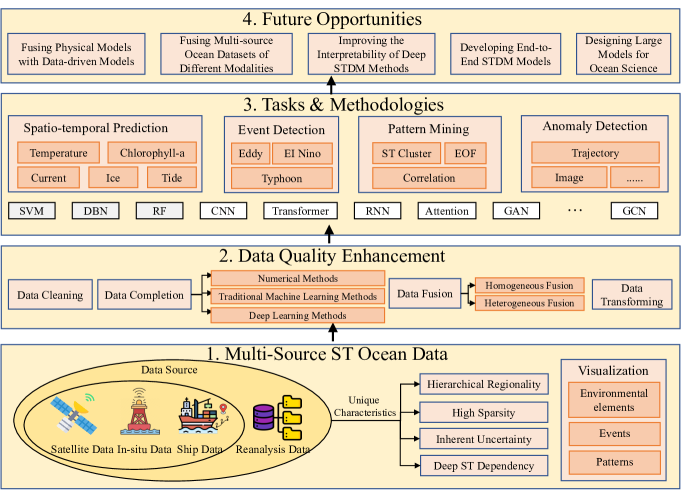
Figure 3. The content and organization of this survey.

Third, STDM for ocean science is a typical multi-disciplinary research field, where rapidly evolving computer science meets conventional ocean science. The development of STDM for ocean science will not only help computer scientists identify new research issues, but also assist the researchers of ocean science in applying advanced STDM methods to solving their problems, which could benefit various oceanic applications. However, the existing and ever-arising challenges and opportunities of STDM for ocean science are not well studied. For example, most existing methods only directly apply STDM methods to addressing ocean issues with large amounts of ST ocean data, ignoring the underlying physical laws of the ocean, which usually lack robustness and interpretability (Haghbin et al., 2021; Wu et al., 2022). Thus, to further promote the development of STDM for ocean science, it is urgent to systemically and comprehensively summarize the related STDM studies for ocean science, and discuss their advantages and disadvantages to help researchers both in computer science and ocean science areas identify potential directions for further exploration.

Keep these in mind, in this paper, as shown in Fig. 3, we provide a comprehensive survey to systematically summarize the available ST ocean datasets, data quality enhancement methods, and STDM techniques for solving various ocean issues, and highlight the arising challenges. In summary, the contributions of this survey are fourfold as follows:

• Summarizing the wide-used and accessible ocean datasets. We review different categories of ST ocean data, including satellite data, in-situ data, ship data, and reanalysis data, and present the popular datasets that are widely used from multiple dimensions (e.g., spatial resolution, temporal coverage, and related studies). In addition, we identify the unique data characteristics of ST ocean data and discuss typical data visualization methods.

• Reviewing the quality enhancement methods for ST ocean data. We analyze the fundamental but necessarily important data quality enhancement methods, including data cleaning, data completion, data fusion, and data transforming for ST ocean data, and provide the corresponding representative models.

• Classifying the advanced STDM methods of typical ocean tasks. This survey provides a comprehensive overview of the recent advances in STDM techniques for ocean science, and subsumes the main tasks into four types, i.e., ST prediction, event detection, pattern mining, and anomaly detection. For each type of these tasks, we provide a detailed review of the corresponding STDM techniques.

• Pinpointing the existing challenges and future directions. We also identify the open problems that have not been well solved and provide some promising research directions in the future, which could help researchers in both computer science and ocean science identify new research topics and promote the development of smart ocean.

The rest of this survey is organized as follows: Section 2 presents different categories of ST ocean datasets, identifies their unique characteristics, and provides typical ST ocean data visualization methods. Section 3 summarizes the techniques for improving the quality of ST ocean data, including data cleaning, data completion, data fusion, and data transforming. Section 4 classifies typical STDM tasks for ocean science into four types and presents a gallery of the technologies for each task. Section 5 discusses the existing challenges and suggests future potential directions. We finally conclude this survey in Section 6.

2. Data Sources, Unique Characteristics and Visualization

In this section, as shown in Table 2, we first summarize four categories of ST ocean data, i.e., satellite data, in-situ data, ship data, and reanalysis data, according to the data sources, and present the representative datasets with their basic information, including temporal periods, spatial resolution, spatial coverage, temporal resolution, and accessible storage. After that, we identify four unique data characteristics of ST ocean data, enabling researchers to understand the key difficulties in applying STDM techniques to solving ocean issues. Finally, the widely-used visualization methods for ST ocean data are discussed.

2.1. Multi-source ST Ocean Data

Typically, existing ST ocean data covers various ocean factors such as temperature, chlorophyll-a, ocean current, sea ice, and tide. The majority of these data are collected by various measurement devices (e.g., satellite sensors, in-situ sensors, and ship sensors) or from the outputs of reanalysis systems (e.g., ECMWF reanalysis system and NOAA reanalysis system). According to the data sources, ST ocean data can be divided into four categories, including satellite data, in-situ sensor data, ship data, and reanalysis data. Table 2 briefly summarizes the advantages and disadvantages of the four categories of ST ocean data. The satellite data and reanalysis data usually have wide spatial coverage and a long-term observation period but have low timeliness to obtain the original data. The ship data and in-situ sensor data have better timeliness but lower data quality due to the data sparsity issue. In this section, we will introduce the typical and commonly used ST ocean datasets of the four data categories and summarize their features in Table 3.

Table 2. Comparison of different categories of ST ocean data.

Category	Spatial coverage	Temporal coverage	Spatial resolution	Temporal resolution	Quality	Timeliness
Satellite data	global	long	low	days	medium	low
In-situ data	local	short	high	hours	medium	high
Ship data	local	short	high	minutes	low	medium
Reanalysis data	global	long	low	days	high	low

Table 3. Public datasets and their features.

Category	Name	Period	Spatial Resolution	Coverage	Temporal Resolution	Citation	Type	Source
Satellite Data	MODIS	2000 to present	0.041x0.041	Global	8 days	(Koner, 2019; Huang et al., 2021a; Hussein et al., 2021; Koner, 2020)	Sea surface temperature, ocean color, sea surface salinity	https://modis.gsfc.nasa.gov/
		2002 to present	1 km x 1 km	Global	daily	(Vazquez-Cuervo et al., 2019)
		2002 to present	0.083°x 0.083°	Global	monthly	(Kilpatrick et al., 2015, 2019)
	AVHRR	1979 to present	1.1 km x 1.1 km	Global	daily	(Koner, 2019; He et al., 2003; Hosoda and Sakaida, 2016)	Sea surface temperature, ocean color	https://www.eumetsat.int/avhrr
	Sentinel-3	2016 to present	1.2 km x 1.2 km	Global	5 days	(Huber et al., 2023; Binh et al., 2022; Fernández-Beltran et al., 2022; Lian et al., 2022; Boy et al., 2022; Xu and Liu, 2022; Liu et al., 2022)	Sea surface temperature, ocean color	https://sentinels.copernicus.eu/web/sentinel/
	GOCI	2010 to 2021	0.5 km x 0.5 km	Korean sea	houtly	(Yeom et al., 2022; Park and Park, 2021; Sun et al., 2019; Liu et al., 2017b)	Sea surface chlorophy-ll, ocean color	https://oceancolor.gsfc.nasa.gov/data/goci/
	CZCS	1978-1986	0.825 km x 0.825 km	Global	8 days	(Zhang et al., 1996; Mukai et al., 1992; Rao et al., 2005; Mélin et al., 2022)	Sea surface chlorophy-ll	https://oceancolor.gsfc.nasa.gov/data/CZCS/
	OCM-2	2009 to present	1-4 km x 1-4 km	Global	2 days	(Rao et al., 2005)	Ocean color	https://ioccg.org/sensor/ocm-2/
	SeaWIFS	1997-2010	1-4 km x 1-4 km	Global	daily	(Mélin et al., 2022; Wang et al., 2019; Li et al., 2015a; Chen and Gao, 2013)	Ocean color	https://oceancolor.gsfc.nasa.gov/SeaWiFS/
In-situ data	Argo	1996-present	Trajectories of about 14060 floats	Global	1-10 days	(Banks et al., 2012; Bhaskar and Jayaram, 2015; Chen et al., 2022; Xue et al., 2022; Xiao et al., 2022)	sea surface temperature, sea surface salinity	https://argo.ucsd.edu/
	GO-BGC	2021-present	Trajectories of about 500 floats	Global	10 days	(Xing et al., 2020; Shu et al., 2022; Cai et al., 2019; Hu et al., 2023)	Sea $O_{2}$, sea Ph	https://www.go-bgc.org/
	SOCCOM	2004-present	Trajectories of about 200 floats	Antarctic Ocean	10 days	(Johnson et al., 2022; Chamberlain et al., 2023)	Ocean carbon	https://soccom.princeton.edu/
Ships Data	AIS	2016 to 2018	Trajectories of about 70,000 vessels	Global	30 seconds - 1 day	(Huang et al., 2021c; Elvidge et al., 2022; Galotto-Tébar et al., 2022; Brandoli et al., 2022)	Trajectory anomalies, ship tracking	https://www.vmsdata.com/
	VMS	April, 2020	Trajectories of 750,000 vessels	Global	30 seconds - 1 day	(Shahir et al., 2019; Storm-Furru and Bruckner, 2020; Guan et al., 2021)	Trajectory anomalies	https://marinecadastre.gov/
Reanalysis Data	OISST	1979-present	0.25°x0.25°	Global	daily	(Zhu et al., 2022; Zhang et al., 2022a; Xie et al., 2022a; Jahanbakht et al., 2022)	Sea surface temperature	https://www.ncei.noaa.gov
	ERA-5	1959-present	4°x4°	Global	12-hour	(Zhang et al., 2022b; McNicholl et al., 2022; Liu et al., 2023; Kuchinskaia et al., 2023)	Sea surface temperature	https://www.ecmwf.int
	CMEMS Level 3 SLA	2004 to present	0.125°x0.125°	Global	daily	(Aouf et al., 2018; Gbagir and Colpaert, 2020)	Sea level anomalies	https://marine.copernicus.eu/
	CMEMS	1993-2020	0.25°x0.25°	Global	daily	(Aouf et al., 2018)	Sea surface height anomaly	https://marine.copernicus.eu/
	HadCRUT4	1961-1990	5°x5°	Global	monthly	(Cowtan and Way, 2014; Morice et al., 2012; Schurer et al., 2018)	Air/Marine temperature anomalies	https://www.metoffice.gov.uk/
	COBE SST	1891 to present	1°x1°	Global	monthly	(Chen et al., 2020; Hausfather et al., 2017)	Sea surface temperature	https://psl.noaa.gov/data/
	COBE-SST 2 and Sea Ice	1850 to 2019	1°x1°	Global	monthly	(Tang et al., 2022), (Chen et al., 2020)	Sea surface temperature, sea ice concentration	https://psl.noaa.gov/data/
	CMAP Precipitation	1979 the present.	2.5°x2.5°	Global	monthly	(Li et al., 2015b; Dong et al., 2023; Kim et al., 2019a)	Pentad global gridded precipitation means.	https://psl.noaa.gov/data/
	WOD	1772 to 2017.	1°x1°	Global	daily	(Boyer et al., 2013)	Sea temperature, salinity, oxygen	https://www.ncei.noaa.gov/products/world-ocean-database

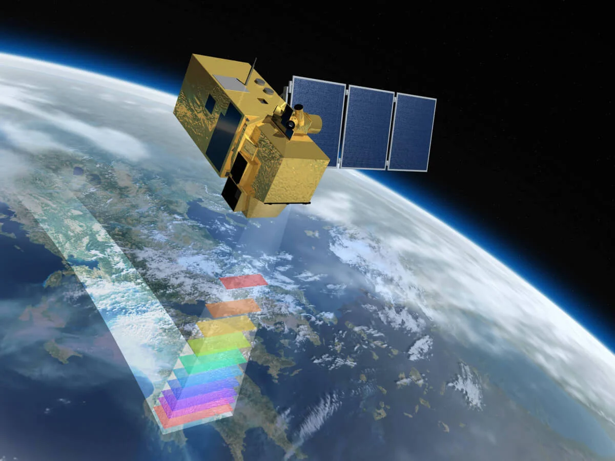
(a) The collection of original satellite data.

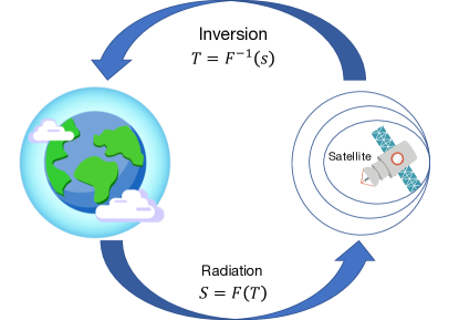
(b) The inversion process of satellite data.

Figure 4. Satellite data collection and inversion. (a) Satellite data collection with different bands (Steve, 2020); (b) Data inversion to process the original satellite data.

2.1.1. Satellite Data

Satellite data, also named remote sensing data, became available in the late 1960s and are a source of high-quality data for monitoring the ocean (Liu and Zhou, 2006). The view from space allows ocean factors  (e.g., SST, and sea surface chlorophyll-a) to be measured globally, especially in remote regions where is not convenient to deploy sensors. Additionally, satellites can ensure large spatial coverage and frequent observation, even in extreme weather conditions. During the past decade, much progress has been made in ocean monitoring using satellites, and the quality of satellite instruments and the accuracy of inversion algorithms have improved considerably, making satellite observations be widely used in various ocean tasks, e.g., sea ice prediction (Zakhvatkina et al., 2019) and typhoon detection (Ruttgers et al., 2018).

As shown in Fig. 4(a), satellite data collection is to detect the thermal energy emitted by the earth’s surface using spaceborne microwave or infrared radiometers (Jiménez-Muñoz and Sobrino, 2003). The surface radiation is modified in its passage through the atmosphere to the radiometer by a bunch of processes, e.g., atmospheric absorption, emission, and scattering. Thus, with appropriate data inversion, we can obtain valid estimates of various ocean factors. The general satellite data inversion process is shown in Fig. 4(b), where $S$ denotes the radiation signal emitted by the ocean surface, and $T$ is the target data obtained by the data inversion function $F$. The data inversion function $F$ is generally non-linear, its inverse function is $F^{-1}$. Through the data inversion algorithms (Liu and Zhou, 2006; Zhang et al., 2009; Shi et al., 2018; Li et al., 2011b), the radiation signal can be transferred to ST time series data of various ocean factors, e.g., SST and sea surface chlorophyll-a.

Many countries have launched satellites for various ocean applications and we introduce the wide-used satellite data as below.

• MODIS: The Moderate Resolution Imaging Spectroradiometer (MODIS) is a key instrument onboard the Earth Observing System (EOS) Terra and Aqua platforms, and designed to monitor the atmosphere, ocean, and land surface. MODIS has a viewing swath width of 2,330 km and views the entire surface of the Earth every two days. It measures 36 spectral bands between 0.405 and 14.385 $\upmu$m, and acquires data at three spatial resolutions, i.e., 0.25km, 0.5km, and 1km.

• AVHRR: The Advanced Very High-Resolution Radiometer (AVHRR) multi-purpose imaging instrument is used for monitoring global cloud cover, sea surface temperature, ice, snow, and vegetation cover characteristics. AVHRR provides four-to-six-band multispectral data from the NOAA polar-orbiting satellite series. AVHRR provides continuous global coverage since June 1979 and its spatial resolution is 1.1 km.

• Sentinel-3: Sentinel-3 is a dedicated Copernicus satellite mission delivering a variety of high-quality ocean and atmosphere measurements. The main objective of the mission is to collect parameters such as sea surface topography, sea surface temperature, and ocean surface color. It provides two-day global coverage optical data with two satellites and altimetry measurements for sea and land applications with real-time data products delivered in less than three hours. The spatial resolution of Sentinel-3 is 1.2 km.

• GOCI: Geostationary Ocean Color Imager (GOCI) is the first ocean color sensor launched to monitor ocean color around the Korean Peninsula. GOCI has a large temporal coverage and it has a revisit time of around 1 hour. The spatial resolution of GOCI is about 0.5 km.

• CZCS: The Coastal Zone Color Scanner (CZCS) is a multi-channel scanning radiometer aboard the ocean remote sensing satellite Nimbus 7. CZCS could map chlorophyll concentration, sediment distribution, salinity, ocean currents, and the temperature of coastal waters. CZCS measures reflect solar energy in six channels at a spatial resolution of 0.8 km.

• SeaWIFS: Sea-viewing Wide Field-of-view Sensor (SeaWiFS) is loaded on the OrbView-2 satellite launched by NASA in 1997. SeaWIFS aims to obtain accurate ocean color data for the global ocean and makes this data readily available to researchers. SeaWiFS has 6 watercolor bands with a bandwidth of 20nm, i.e., 412nm, 443nm, 490nm, 510nm, 555nm, and 670nm. Compared with CZCS, the performance indicators of this sensor have been greatly improved, such as more reasonable band settings, higher signal-to-noise ratio, and richer band information. SeaWiFS has two spatial resolutions, i.e., 1.1 km and 4.5 km, and its temporal resolution is daily or once every two days.

2.1.2. In-situ Sensor Data

In-situ sensor data refers to the data collected where the instrument is physically located. It is a traditional but important way to collect data for ocean factors and has a long history since the 1600s (Faghmous and Kumar, 2014). In the past few decades, numerous in-situ sensors of different types, e.g., buoys sensors, underwater sensors, and station sensors, have been deployed all over the world. However, considering the wide spatial coverage of the ocean, in-situ sensor data are still sparse in space and time since they are only available when and where the sensors are physically located. In addition, due to the data privacy issue, there is only a small portion of in-situ sensor data available to the public. We introduce the three available and widely used in-situ sensor datasets, i.e., Argo, Go-BGC, and SOCCOM, as below.

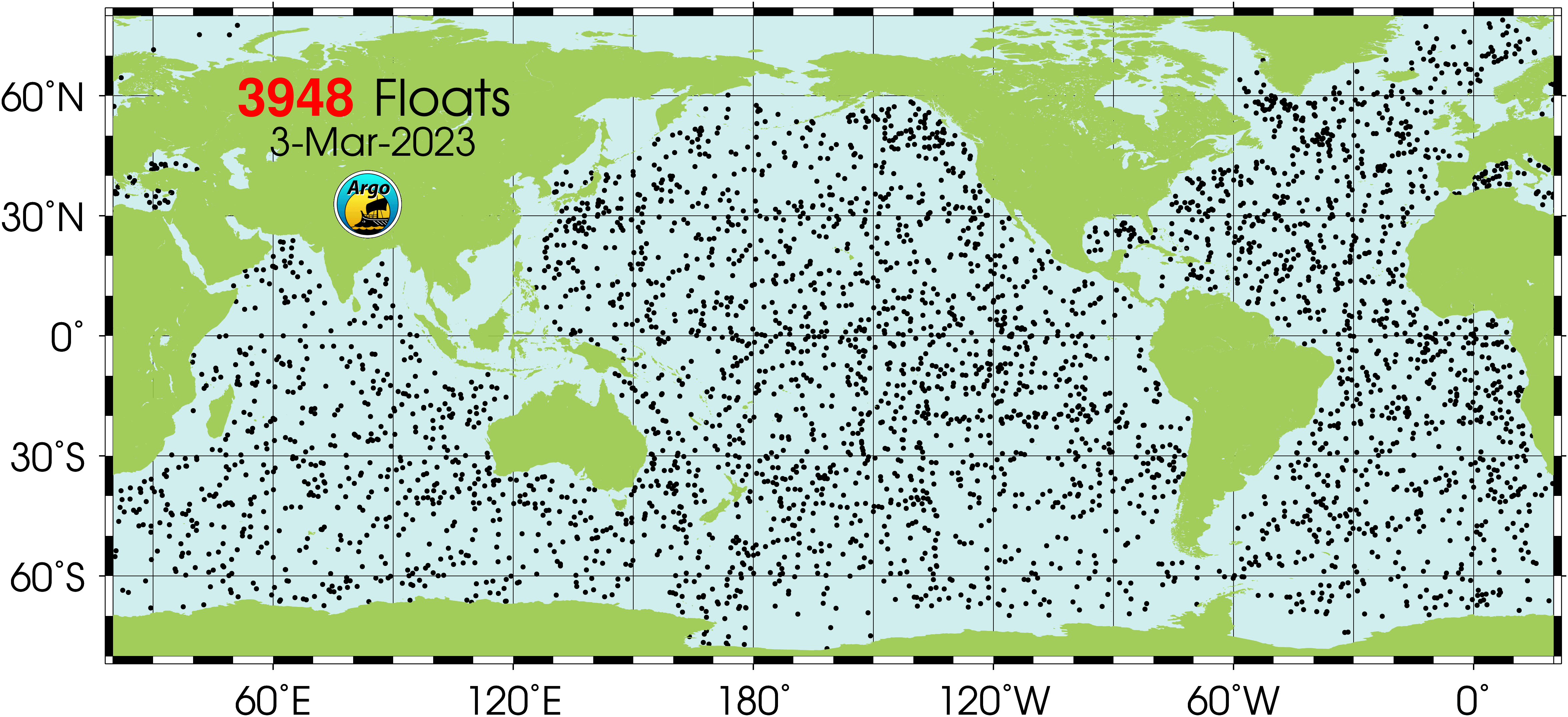
Figure 5. The global distribution of Argo sensors in 2023 (Pic, 2018).

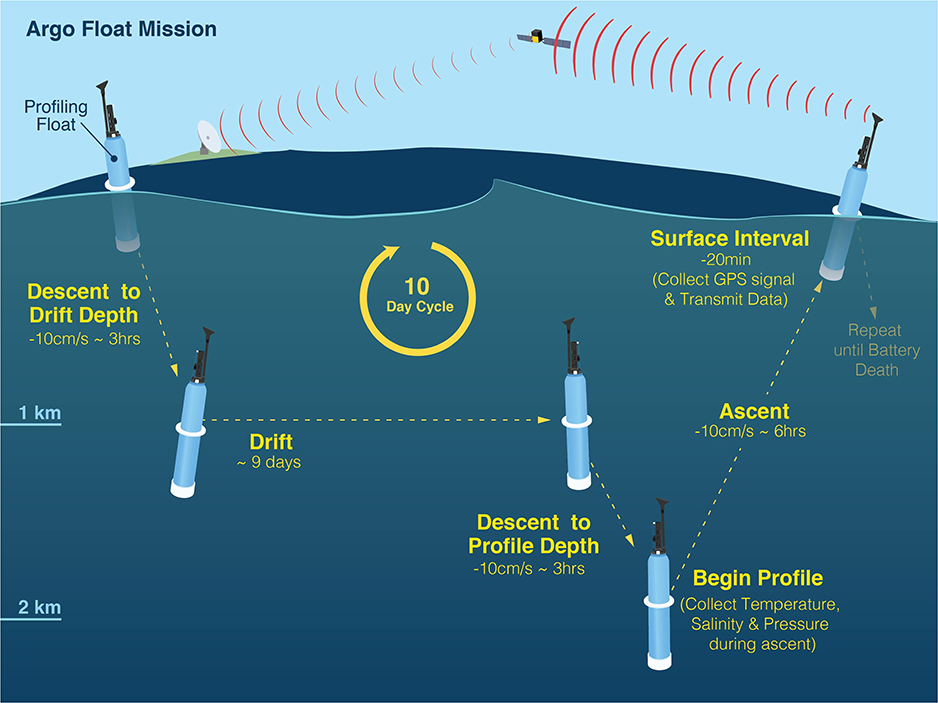
Figure 6. The workflow of Argo sensors (Pic, 2023b).

• Argo: Array for Real-time Geostrophic Oceanography (Argo) is an international program that uses profiling floats to observe temperature, salinity, currents, and other factors in the ocean. It has been in operation since the early 2000s and provides real-time data for studying climate and oceanography. Fig. 6 shows the global distribution of 3948 sensors from the Argo program (Pic, 2018). As shown in Fig. 6, the Argo float mission is a 10-day cycle, and Argo sensors drift at a depth of 1000 meters (the so-called parking depth) and measure the conductivity, the temperature, etc, as it moves back up to the ocean surface. Once the float is on the surface, it will communicate with a satellite and send its location and collected data to them, then continue its mission (around 4-5 years).

• GO-BGC: The Global Ocean Biogeochemistry (GO-BGC) Array is a project to build a global network of chemical and biological sensors on profiling floats. The network monitors biogeochemical cycles and ocean health, including the elemental cycles of carbon, oxygen, and nitrogen through all seasons of the year.

• SOCCOM: The Southern Ocean Carbon and Climate Observations and Modeling project (SOCCOM) is a multi-institutional program focusing on unlocking the mysteries of the Antica Ocean, exploring the influence of carbon, nutrients, oxygen, and other factors on global climate.

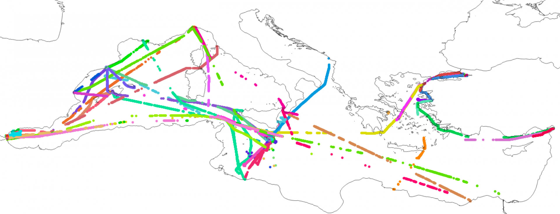
Figure 7. The visualization of ship trajectories in the Automatic Identification System (AIS) (Pic, 2023a).

2.1.3. Ship Data

Ship data is collected by ships and vessels for directly observing the ocean factors, collecting biology samples, and investigating the ocean (Storm-Furru and Bruckner, 2020). Ships can collect marine data at different locations along their trajectories. Here, we introduce two common tracking systems that record the information of ships.

• AIS: Automatic identification system (AIS) is an operation tracking system that provides ships’ information such as the type of ship, location, and speed. Fig. 7 visualizes several AIS trajectories of ships. AIS was used by the U.S. Coast Guard in 2009 for the first time to monitor and transmit the locations of huge vessels. According to International Maritime Organization (IMO), the goals of developing AIS are to help recognize ships, assist in target tracking, enhance the safety of marine traffic, and make the flow of vessel traffic smooth. Since 2004, installing AIS transponders for vessels over 300 tons of weight is mandatory in the International Convention for Safety of Life at Sea (SOLAS) guideline.

• VMS: Vessel Monitoring System (VMS) is a form of satellite tracking using transmitters on board fishing vessels. It tracks vessels in a similar way to AIS but is restricted to government regulators or other fisheries authorities. All European Union, Faroese, and Norwegian vessels which exceed 12 meters overall length must be fitted with VMS units. VMS collects the locations, times, and oceanic features, along the trajectories of vessels.

2.1.4. Reanalysis Data

It is important to have complete observations of the ocean system in both spatial and temporal dimensions. However, the observations discussed above are usually unevenly distributed. Even in satellite data, the observations cannot provide a complete recording of the state of the ocean system across the globe at a given point in time. Reanalysis data is the most completed data, which fills the gaps in the observational records through the simulation models or the physic models (Zhu et al., 2022). Reanalysis datasets are often globally complete and consistent in time, and referred to as ‘maps without gaps’. They are among the most-used datasets in ocean, especially in various data-driven ocean applications. We introduce the two widely-used reanalysis datasets, i.e., ERA5 and OISST, as follows:

• ERA5: ECMWF Reanalysis Atmosphere V5 (ERA5) is published by ECMWF for monitoring the global climate, which provides hourly data with estimates of uncertainty for the parameters of atmospheric, land-surface, and ocean. ERA5 data are available in the Climate Data Store on regular latitude-longitude grids at 0.25°x0.25° resolution, providing atmospheric parameters on 37 pressure levels, sea surface temperature, sea wave height, etc.

• OISST: NOAA’s Optimum Interpolation Sea Surface Temperature (OISST, also known as Reynolds’ SST) is a series of global reanalysis products, including the weekly OISST data on 1°x1° grids and daily OISST data on 0.25°x0.25° grids. OISST generates smoothed and complete ocean observation data by conducting interpolating and extrapolating operations based on a combination of ocean temperature observations from satellites and in-situ platforms (e.g., ships and buoys). The input data is first mapped to specific regular grids since they are usually irregularly distributed in space. Then, statistical methods, e.g., optimum interpolation (OI) (Huang et al., 2021b), are applied to fill in the missing values.

2.2. Unique Data Characteristics

Compared with typical ST data (e.g., traffic flow data and epidemic outbreak data), ST ocean data not only contains ST dependencies between adjacent locations but also has a lot of complex and unique characteristics. Here, we summarize four unique characteristics of ST ocean data as below.

Diverse Regionality. In general, the ocean can be divided into a lot of regions from different aspects. For example, one general partition is based on the climate zones to divide the ocean into various regions, such as tropical zones and frigid zones. On the one hand, each region has diverse patterns from others. For example, the collected ocean data in the Arctic Ocean may have opposite patterns from the data near the equator (Yang et al., 2023). On the other hand, when learning the ST correlations in ocean, it is of high importance to capture the ST correlations between regions since the ocean is a unified system. Moreover, due to the ocean current and atmospheric circulation, the correlations between regions are not static but dynamically changing over time. This regionality brings difficulties for one model to learn the diverse features of all ocean regions, thus requiring adaptive learning for different regions.

High Sparsity. Sparsity is an important characteristic of ST ocean data. For in-situ data and ship data, they are collected in a sparse and uneven distribution in both space and time, which leads to high sparsity in observation data for certain periods and some ocean areas. For satellite data, the collected data may be highly missed due to the cloud covering and the scanning cycle of satellites, and the sensors’ stability and transmission loss. For example, according to (Lian et al., 2023), the missing rate of MODIS satellite data could be higher than 80% in some periods. As a result, it is difficult to obtain continuous, accurate, and uniform ST ocean data in a wide range. In this case, STDM models have to learn knowledge and patterns from incomplete data, which makes the overfitting problem more serious. Thus, how to address the sparsity issue in ST ocean data is an important yet challenging task for developing STDM methods for ocean science.

Inherent Uncertainty. Another characteristic of ST ocean data is the inherent uncertainty due to the instability of the data collection process, which may cause the collected data to contain noise and deviate from real values. Concretely, the uncertainty in ST ocean data stems from the fact that many ocean datasets have biases in sampling and measurement. For instance, uncertainty might occur because a particular thermometer is miscalibrated or poorly sited. However, data producers seldom provide uncertain information about data. For example, one may have access to three different SST datasets: one reanalysis dataset at 2.5°x 2.5° spatial resolution, another dataset at 0.75°x 0.75° spatial resolution, and a satellite dataset at 0.25°x 0.25° spatial resolution. Given that each dataset has its own biases, how to effectively fuse these datasets to obtain the correct information remains a challenging issue.

Deep Spatial-temporal Dependency. With the wide spatial coverage of the global ocean and long-term temporal record, ST ocean data has more complex and deep ST dependencies than typical ST data. Concretely, from the spatial view, the wide spatial coverage brings complicated ST dependencies between different ocean locations. For example, the well-known El Ni$\mathrm{\tilde{n}}$o event, occurring in the equatorial Pacific Ocean, has been proven to cause intense storms and extreme temperatures in many regions far away from the Pacific Ocean via the tropical tropospheric and atmospheric bridge mechanism (Yang et al., 2018b). From the temporal view, ST ocean data may have long-term temporal dependencies and short-term dependencies, which requires STDM methods to have the capability to model such hierarchical temporal dependencies. For example, SST shows a certain cyclical pattern in the year, and the SST in winter is usually differently distributed from that in summer. In addition, the spatial dependency and temporal dependency in ST ocean data are often entangled, which makes learning the ST dependencies a non-trivial task.

2.3. Data Visualization

Visualization of ocean data is important for scientists and engineers to understand various ocean phenomena and discover their underlying complex and dynamic patterns. Since interactive visual analysis integrates the experts’ knowledge into the design of the models and algorithms (Li et al., 2011a), it allows us to interactively explore, analyze and assess data at different spatial-temporal scales to gain more insights into the data than traditional ways of data analysis. We introduce three typical types of visualization methods for ST ocean data as below.

• Ocean environmental elements visualization. Ocean environmental elements are a number of basic physical properties that affect the ocean ecosystem, including scalar data (e.g., temperature and salinity) and flow fields (e.g., trajectories and ocean currents). 2D plots (e.g., points, lines, surfaces, particles, and glyphs) and 3D volume rendering are widely-used methods for the visualization of these ocean environmental elements. For example, Fig. 8 visualizes the global SST at different depths and the distribution of global surface ocean pH. Currently, with the rapid development of hardware technology, the GPU-based hybrid graphics visualization approach is popular (Li et al., 2011a). Su et al. (Su et al., 2016) developed an ocean data visualization system that supports line contouring, volume rendering, and dynamic simulation of the sea current field. The system employs GPU-based rendering to visualize scalar or flow fields efficiently and is used for monitoring the changing processes of ocean environmental elements. Liu and Chen (Liu et al., 2017a) also developed a framework for interactive visual analysis of heterogeneous marine data. Ocean environmental elements visualization could help us well understand the inherent operating processes of the ocean system.

  

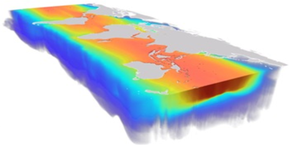
  (a) The visualization of global SST at different depths.

  

  (b) The visualization of global surface ocean pH.

  Figure 8. The visualizations of ocean environmental elements: (a) The global SST at different depths (Pic, 2020), and (b) the global surface ocean pH from two different analysis projects (Jiang et al., 2019).

  

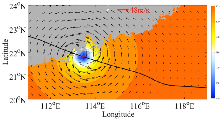
  Figure 9. The visualization of typhoon Hato at 04:00 UTC on 23 August 2017, where the black line shows the path of Hato (Du et al., 2020).

  

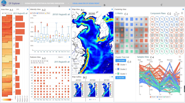
  Figure 10. The interface of OFExplorer, a visualization tool for exploring and discovering SST characteristics and patterns (Xie et al., 2022b).

• Ocean event visualization. The interaction between various ocean environmental elements constitutes a variety of ocean events. For instance, ocean eddies, ocean fronts, typhoons, and EI Ni$\mathrm{\tilde{n}}$o are common events occurring in the ocean, which often last for several days to several months. Each event has different characters and needs special algorithms for visualization. Various methods have been proposed to visualize these events. For example. Fig. 10 visualizes the trajectory of typhoon Hato in 2017. George et al. (George et al., 2014) proposed a framework for the visual analysis of the sea level rise event, and provided multiple visual analytic tools for interactive hydrodynamic flux calculation on spatial-temporal and multivariate data. Hollt et al.(Hollt et al., 2014) developed an interactive visualization system for sea surface height data to support interactive exploration and analysis of the spatial distribution and the temporal evolution of ocean eddies. In general, the spatial and temporal scales of ocean events are often different, which requires event visualization methods to be adaptable to changeable scales (Köthur et al., 2014).

• Ocean pattern visualization. Ocean patterns are related to complex ocean processes, which are hidden in the spatial and temporal variability of ocean data. ST pattern visualization is used for understanding the evolution characteristics of the ocean environmental elements (e.g., temperature and salinity) or phenomena (e.g., eddies and fronts) over time to detect trends, periodicity, and other important factors. For example, Xie et al. (Xie et al., 2022b) developed the visualization tool OFExplorer, as shown in Fig. 10, to discover the changing patterns of SST. Another ocean pattern visualization approach integrates the changes of ocean environmental elements in both time and space into a 3D volume rendering (Resch et al., 2014) by reducing the feature dimension through slicing, averaging, and aggregation operations, or using PCA-like methods (Sacha et al., 2017; Sips et al., 2012).

3. Data Quality Enhancement

High data quality is of great significance to ensure that the results of STDM are reliable, accurate, and complete (Kim et al., 2020). However, in practice, it is difficult to get ST ocean data with high quality for many reasons such as the limited spatial and temporal coverage, the failures of data collection devices, and the loss during data transmission and storage. Meanwhile, the diversity of the data sources and the big volume of ST ocean data also seriously affect the quality of ST ocean data. Therefore, to address the data quality issue, a number of studies have been conducted on data quality enhancement, which can make ST ocean data more suitable for specific applications. In this section, we overview three foundational data processing operations, i.e., data cleaning, data completion, and data fusion, and the corresponding techniques to improve the quality of ST ocean data. In addition, we introduce the data transforming process, which aims to transform the data representation to meet the specific requirements of the STDM tasks.

3.1. Data Cleaning

Data cleaning aims to remove incorrectly formatted data which may result in inaccurate analysis and unreliable results. Data cleaning requires a good understanding of the real distributions and statistical implications of the original data. Existing methods, e.g., statistical analysis methods, proximity measurement methods and density-based clustering methods, for data cleaning usually use constraints, rules, and patterns to detect and remove the outliers in data (Zhou et al., 2020). Statistical analysis methods (Dasu and Loh, 2012) detect the outliers that do not follow the given data distributions or regression equations. Proximity measurement methods first define a proximity measure between data points and then identify those abnormal data points that are far away from the other data points. Density-based clustering methods (Duan et al., 2009) detect the data outliers by comparing their local density with the neighboring data points and are suitable for non-uniformly distributed data. For the ST data in ocean, we utilize the above methods to remove the incorrectly formatted data points and improve the data quality for downstream STDM tasks.

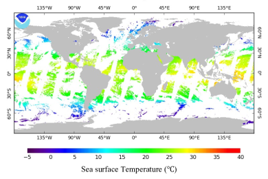
(a) The spatial distribution of SST records from AVHRR satellite data on 3 October 2021, where the white areas have no data, and the gray areas are lands (Pic, 2021a).

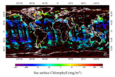
(b) The spatial distribution of Chl-a records from MODIS satellite data on 3 October 2021, where the black areas have no data (Pic, 2021b).

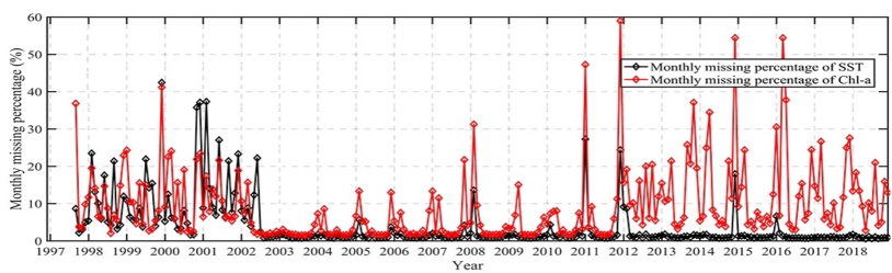
(c) The monthly missing percentages of SST and Chl-a in the area of Northern South China Sea from 1997 to 2018 (Ma et al., 2021).

Figure 11. Distributions and missing rates of global SST and Chl-a data. (a) / (b) The spatial distribution of SST / Chl-a records from AVHRR / MODIS satellite data on 3 October 2021, and (c) the monthly average missing rates of SST and Chl-a in the Northern South China Sea from 1997 to 2018.

3.2. Data Completion

The issue of data missing or sparsity is very common in ST ocean data due to the influence of various inevitable factors such as cloud occlusion, bad weather, and sensor failure. If missing values are not well treated, the data analysis results may be unreliable and inaccurate, leading to bias in further applications. As shown in Fig. 11(a) and Fig. 11(b), due to the cloud occlusion, both AVHRR data and MODIS data have many missing values. According to Fig. 11(c), the monthly missing rate of MODIS data in the Northern South China Sea is often between 20% and 50% and the missing rate of SST even reaches 60% in 2012, let alone the daily data missing rates. Apparently, compared with typical ST data such as traffic data and crowd volume data, the missing rate in ocean data is extremely high, making it difficult to conduct data analysis and restricting the development of real-world applications (e.g., weather forecasting and typhoon detection). Therefore, data completion is regarded as a necessary step in ST ocean data quality enhancement and a variety of data completion methods have been proposed. In this section, we briefly introduce the problem definition of data completion and the related techniques.

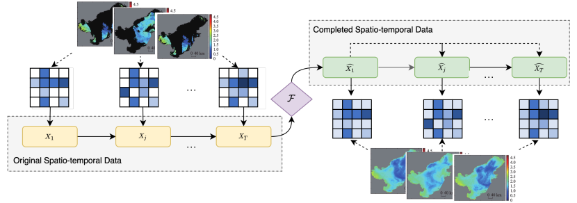
Figure 12. The general framework of ST data completion, where the input is incomplete ST data, the output is completed data, and $\mathcal{F}$ could be various data completion algorithms.

As shown in Fig. 12, we use matrix $X=(X_{1},...,X_{j},...,X_{T})\in{{\mathbb{R}}^{N\times T}}$ to represent the time-series of recorded ocean data for $N$ nodes (e.g., grid ocean regions and sensor locations) at $T$ timestamps, where $X_{j}$ represents the observation values for all nodes at timestamp $\tau_{j}$, and $x_{i,j}$ is the observation value of node $v_{i}$ at timestamp $\tau_{j}$. In addition, a masked matrix $M=(M_{1},...,M_{j},...,M_{T})\textbf{}\in{{\mathbb{R}}^{N\times T}}$ is introduced for $X$, where each entry $m_{i,j}=0$ if the entry $x_{i,j}\in X$ is missing, otherwise $m_{i,j}=1$.

Given the incomplete data matrix $X$ and its masked matrix $M$, the data completion problem aims to fill the missing values in $X$ and ensure that the filled values are close to the real values, i.e.,

(1) $${{\widehat{X}}}=\bm{\mathcal{F}_{\theta}}\{{{X}},{M}\},$$

(2) $${{\widetilde{X}}}={{X}}+{{\widehat{X}}}\odot\left({\mathrm{O}}-M\right),$$

where ${{\widehat{X}}}$ is the generated data matrix by data completion model function $\bm{\mathcal{F}}$, $\theta$ denotes all the learnable parameters in the model, ${\mathrm{O}}$ is a matrix whose entries are all ones, and $\odot$ denotes Hadamard product. Finally, we can get the completed data ${{\widetilde{X}}}$.

Existing ST data completion methods can be roughly divided into three categories, i.e., numerical methods, traditional machine learning-based methods, and deep learning methods. And the summarization and comparison of these methods are in Table 4.

Table 4. Major existing methods of ocean data completion.

Category	Strengths	Weaknesses	Model	Year	Approach
Numerical methods	Need a small amount of data, simple, fast, flexible, and adaptable.	Cannot model non-linear data, depend on a correct domain knowledge.	OI (Huang et al., 2021b)	1987	min-variance
			Kriging  (Oliver and Webster, 1990)	1990	linear combination of nearby data
			IDW (Bartier and Keller, 1996)	1996	averaging neighbors’ data
			DINEOF (Alvera-Azcárate et al., 2005)	2005	Empirical Orthogonal Function (EOF)
Traditional machine learning based methods	Can model dynamic, non-linear, and noisy data, easy to set up, self-adaptable, self-organizing, and error tolerant.	Have a high computational cost and tend to overfit when applied to long-term data.	RF (Park et al., 2020)	2006	a multitude of decision trees
			XGBoost (Shen et al., 2018)	2014	gradient boosting decision trees
			ANN (Pisoni et al., 2008)	2015	artificial neural network
			KNN (Hu et al., 2021)	2013	averaging k-nearest neighbors
			SOM (Jouini et al., 2013)	2013	self-organizing map
			SVR (Mohebzadeh et al., 2021)	2005	calculating the best model to fit points
			MF (Liu and Li, 2022)	2006	matrix decomposition
Deep learning methods	Extract deep features from the data, can work with noisy data, captures temporal dependencies over variable periods of time, high accuracy.	High complexity, high computational cost, need to be tuned carefully lack of interpretability	NN (Jamet et al., 2012)	2012	neural network
			CNN (Vient et al., 2021)	2020	convolutional neural network
			DINCAE (Jouini et al., 2013)	2016	convolutional auto-encoder
			GAN (Pan et al., 2021)	2021	generative adversarial network
			GCN (Lian et al., 2023)	2022	graph completion network
			STA-GAN (Wang et al., 2022b)	2023	generative adversarial network

3.2.1. Numerical methods

Numerical methods learn the linear correlations from past observations and the domain knowledge  (e.g., physical laws of the ocean) to achieve data completion. History average (HA) only uses the average of past data to fill in the missing values, which is too simple to learn the non-linear relationships. To simulate the true data distribution, the Optimal Interpolation (OI) method (Huang et al., 2021b) uses the min-variance to obtain the ideal unbiased approximation of missing data and is widely used to build cloud-free SST products by fusing data from multiple platforms, such as satellite data, in-situ data, and ship data. For example, the OI method is employed in the NOAA OISST products (Huang et al., 2021b) and the blended foundation SST products (Hosoda and Sakaida, 2016). In addition, the OI method is popular for analyzing daily SST by fusing the AVHRR satellite data and the Tropical Rainfall Measuring Mission Microwave Imager products (He et al., 2003). Distance-based data completion methods fill the miss data with the average of the data within a certain physical distance and are also popular in the early ages. For example, Kriging (Bhattacharjee et al., 2014; Lu and Wong, 2008) and IDW (Shen et al., 2018)) achieve good performance on SST data completion based on the spatial relevance of original data. Beckers proposed the DINEOF method (Beckers and Rixen, 2003) to achieve missing value completion in oceanographic data based on the Empirical Orthogonal Function (EOF). DINEOF is widely used for the completion of Chl-a data (Liu and Wang, 2018; Guo et al., 2022), SST data (Li et al., 2021b; Ma et al., 2021), ocean wind data (Zhao et al., 2010) and multivariate ocean factors (Alvera-Azcárate et al., 2007).

In practice, numerical methods are simple and flexible, and widely used for filling in missing values in various ocean data products. However, they cannot well learn the complex nonlinear relationships in ocean data, and some methods are highly dependent on expert knowledge to set the values of parameters, which is not sufficient to achieve accurate ST data completion.

3.2.2. Traditional machine learning-based methods

Traditional machine learning-based methods aim to utilize historical ocean data to train machine learning models to simulate data distributions for data completion. Various machine learning methods, e.g., Random Forest (RF), eXtreme Gradient Boosting (XGBoost), and Matrix Factorization (MF), have been applied for ST ocean data completion (Hu et al., 2021; Mohebzadeh et al., 2021; Park et al., 2019). Shen et al. (Shen et al., 2018) utilize the RF method to fill the missing values in satellite data by constructing multiple decision trees. Chen et al. (Chen et al., 2019a) used RF to improve the coverage of Chl-a data with two external factors, i.e., the Ocean Color Index and the Rayleigh-corrected Reflectivity. Hu et al. (Hu et al., 2021) proposed an RF method with XGBoost to complete the sea surface Chl-a data. KNN and SVR have been also adopted to fill missing values of ocean data based on distance measurement (Sunder et al., 2020; Mohebzadeh et al., 2021; Hu et al., 2021). Jouini et al. (Jouini et al., 2013) proposed the Self-Organizing Map (SOM) network to complete Chl-a data under heavy cloud coverage by integrating SST and sea surface height (SSH). Artificial Neural Network (ANN) is applied for the completion of SST data in the Mediterranean (Pisoni et al., 2008). Hankel Matrix Factorization (HMF) is introduced for data completion in the Global Navigation Satellite System (GNSS) (Liu and Li, 2022).

In sum, traditional machine learning-based methods are easy to set up, have the ability to model the dynamic, non-linear, and noisy features of ST ocean data, and also achieve good performance on short-term data. However, they have a high computational cost, tend to overfit when applied to long-term data, and cannot well capture the complex ST dependencies in ocean data.

3.2.3. Deep learning-based methods

To capture the complex ST dependencies, deep learning-based data completion methods have been introduced to improve the quality of sparse ST ocean data. For example, the Neural Classification method is proposed for filling the cloud covering values in SST data (Jouini et al., 2013). Jean-Marie (Vient et al., 2021) achieved the completion of SST data using a neural network (NN) and proved that the NN is superior to the OI and EOF methods. Zhao et al. (Zhao et al., 2023b) proposed an LSTM-based method to fill the missing values of wave height data. Barth et al. proposed the Data-Interpolating Convolutional Auto-Encoder (DINCAE) for the completion of Chl-a data (Barth et al., 2020) and SST data (Han et al., 2020b). Generative Adversarial Imputation Network (GAIN) (Pan et al., 2021) with different generation rules has been introduced for missing data completion, and can effectively learn the complex data distribution. GCN-based models (Lian et al., 2023) have been adopted to utilize an algebraic framework termed Graph-Tensor Singular Value Decompositions (GT-SVD) to extract hidden spatial information in ocean monitoring data. Wang et al. (Wang et al., 2022b) combined attention and GCN (Wang et al., 2022b) to capture both short-term temporal dependence and dynamic spatial dependence in ST ocean data and achieved good performance in satellite data completion. Moreover, the diffusion model has been applied in this field due to its superior generative ability. Tashiro et al. (Tashiro et al., 2021) proposed a score-based diffusion model for filling incomplete values and developed a self-supervised training method by using available observation values to train the model.

Deep learning-based data completion algorithms could achieve high accuracy in ST ocean data completion and can capture dynamic dependencies over time. However, they still have some weaknesses. First, deep learning-based data completion algorithms are of high complexity, and their training and tuning processes are time-consuming. Besides, the deep learning methods are treated as ”black boxes” and have low interpretability. Therefore, it is still worth exploring to reduce the time complexity of deep ST ocean data completion methods and enhance models’ interpretability in the future.

3.3. Data Fusion

For many STDM tasks, e.g., climate forecasting and typhoon tracking, multi-source ocean data collected by various producers, e.g., NOAA, NASA, and ECMWF, are required to obtain comprehensive knowledge. These different datasets usually have diverse data collecting standards, equipment, and technologies, leading to different ST resolutions, different ST coverage, and different data quality. For example, in-situ observations can provide precise information about the ocean at specific locations, but they have issues of sparsity, uneven distribution, and low resolution. Meanwhile, satellite data can provide continuous observation of the ocean over a wide area and for long periods, but is unable to obtain fine-grained information at the location level. Therefore, how to combine the benefits of multi-source observation data to build high-quality ST ocean datasets is an important yet challenging problem. Specifically, for STDM in ocean, data fusion is to integrate multiple data sources to obtain more comprehensive and consistent information about the ocean. Existing methods for fusing multi-source ST ocean data can be roughly classified into two categories, i.e., homogeneous data fusion methods and heterogeneous data fusion methods.

3.3.1. Homogeneous data fusion methods

Homogeneous data fusion aims to combine the datasets from the same source into a comprehensive dataset to improve the data quality. At early ages, the most common way to fuse homogeneous data is to utilize their statistical characteristics (e.g., local mean matching, regression analysis, and statistical region merging) (Cressie, 1996). However, it is difficult to fuse the observation records of two datasets from the same source with different spatial and temporal scales. To solve this problem, Nguyen et al. (Nguyen et al., 2012) presented the spatial data fusion methodology based on the spatial-random-effects model, where the spatial distribution is learned based on the data of different temporal scales within the same region. Kang et al. (Ma and Kang, 2020) proposed the Dynamic Fused Gaussian Process (DFGP) to combine a low-rank representation with a general covariance matrix with a dynamic-statistical approach to fuse the satellite data from different sensors. Jung et al. (Jung et al., 2022) utilized the RF to fuse two satellite datasets to acquire high-quality SST data. To extract fine-grained data information from ocean data, many researchers utilize deep learning methods to learn the data embedding to fusion the data for downstream tasks (e.g., SST prediction). Hou et al. (Hou et al., 2022) proposed an ST ocean data fusion model based on ConvLSTM to combine three different satellite datasets and achieve good SST prediction results. Raizer et al. (Raizer, 2013) proposed a digital wavelet transform method for combining the information in both spatial and temporal domains on two satellite datasets.

3.3.2. Heterogeneous data fusion methods

Heterogeneous data fusion aims to combine data from different data sources, thus providing more comprehensive information than the dataset from a single source. Due to the variety in form and content across spatial and temporal scales, it is much more difficult to fuse heterogeneous data than homogeneous data. Wikle and Berliner (Wikle and Berliner, 2005) proposed a hierarchical Bayesian model to fuse the satellite data with reanalysis data by adjusting the data of different spatial resolutions with its areal-averaged data. McMillan et al. (McMillan et al., 2010) proposed an ST model that combines in-situ observations and the reanalysis model’s gridded outputs by assuming that the data collected at the same location has the same data distribution. Chen et al. (Acharya et al., 2017) provided a Bayesian inference model to fuse the in-situ data and satellite data for the accurate estimation of chlorophyll-a. Han et al. (Han et al., 2021b) proposed a CNN-based fusion algorithm to combine the satellite image data and time-series data and achieved good performance in downstream applications. Wang et al. (Wang et al., 2023) provided an ODF-net to fuse in-situ observations, satellite observations, and reanalysis data with a self-training attention mechanism.

In conclusion, fusing multi-source data can enhance data consistency and quality, and improve the accuracy of STDM tasks for ocean science. However, existing methods for fusing ST ocean data usually rely heavily on prior statistical knowledge of linear principles, normal distributions, and error covariances. In addition, these methods are often tailored for specific datasets and tasks, and there are no unified data fusion frameworks that can fuse various ST ocean data sources. These limitations are still open issues that need further exploration.

3.4. Data Transforming

In practice, different ocean application scenarios correspond to different categories of STDM tasks and problem formulations, and different STDM tasks usually have different requirements for the formats of input data. Therefore, the original data from multiple sources cannot be directly used for various STDM tasks. An important process before putting data into STDM models is to transform the data to meet the specific requirements of the data mining task. As shown in Fig. 13, we provide a clear mapping from different data sources to different data instances (i.e., ST points, Trajectories, Time series, and ST raster) and four types of tasks (cf. Section 4 for the details). For example, an ST point refers to a tuple containing spatial and temporal information as well as ocean features (e.g., temperature and chlorophyll-a), which can be obtained by in-situ sensors and ship sensors. Then, a series of ST points collected at different locations can be utilized for detecting various events (e.g., El Ni$\mathrm{\tilde{n}}$o and typhoon). A trajectory, usually collected by a sailing ship or moving sensor, consists of the continuous measurements of an ST feature over a set of moving reference points in space and time and can be utilized in ship anomaly detection, and pattern mining tasks. ST raster data refers to the measurement of a continuous or discrete ST field recorded at fixed locations in space and at fixed points in time, which is usually collected by the satellite sensors and obtained from the outputs of reanalysis models. ST raster data is an important data format for STDM tasks and also can be transformed into other data instances (e.g., ST points and time series) for different tasks.

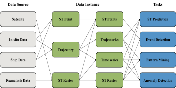
Figure 13. A mapping from the data sources to the data instances and the four types of ocean STDM tasks.

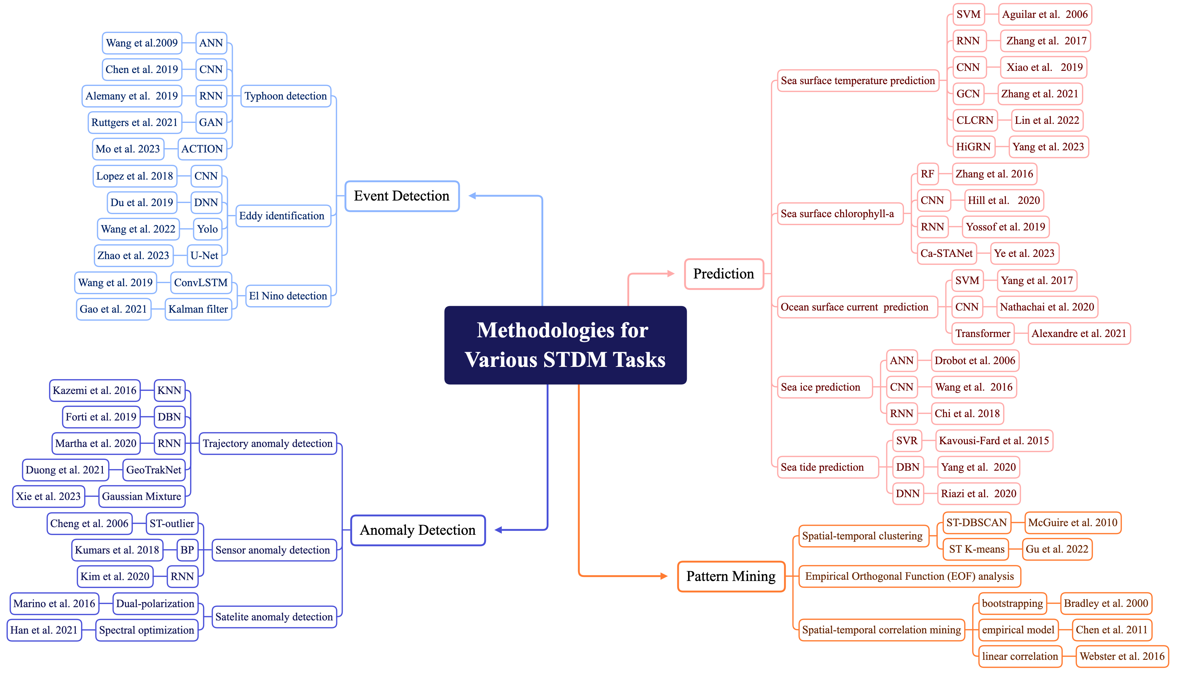
Figure 14. A taxonomy of methodologies of different ocean STDM tasks.

4. Tasks & Methodologies

As shown in Fig. 14, to provide a clear overview of the STDM techniques for ocean science, we classify the STDM tasks in ocean into four typical categories, i.e., prediction, event detection, pattern mining, and anomaly detection, based on the problem formulation. And Fig. 15 illustrates the distribution of published research papers on these tasks, among which SST prediction and typhoon detection are the most popular. In addition, Table 5 further presents the representative tasks for each category of STDM tasks.

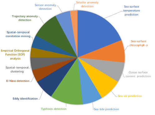
Figure 15. The distribution of publications of various ocean STDM tasks (data from the Web of Science.

Table 5. Representative ocean STDM tasks.

Task Categories	Tasks	Related studies
Spatial-temporal Prediction	Sea surface temperature prediction	(Repelli and Nobre, 2004),(Storto and Masina, 2015),(Storto et al., 2016),(Buongiorno Nardelli et al., 2013),(Zivot and Wang, 2003), (Zhang, 2003), (Xue and Leetmaa, 2000),(Aguilar-Martinez and Hsieh, 2009),(Lins et al., 2013), (Wu et al., 2006), (Zhang et al., 2017), (Yang et al., 2018a),(Zhang et al., 2020),(Krizhevsky et al., 2012),(Xiao et al., 2019),(Hou et al., 2021),(Zhang et al., 2022a),(Sun et al., 2021), (Haghbin et al., 2021), (Acharya et al., 2017), (Koner, 2019),(Hussein et al., 2021) .
	Sea surface chlorophyll-a prediction	(Kiyofuji et al., 2006),(Liu et al., 2010),(Recknagel et al., 2002), (Zhang et al., 2016),(Hill et al., 2020),(Yussof et al., 2021),(Lee and Lee, 2018),(Wang and Xu, 2020),(Hussein et al., 2021).
	Ocean surface current prediction	(Frolov et al., 2012),(Barrick et al., 2012),(Sarkar et al., 2018),(Guozhen et al., 2017),(Remya et al., 2012),(Sarkar et al., 2019),(Immas et al., 2021),(Thongniran et al., 2019).
	Sea ice prediction	(Zakhvatkina et al., 2019),(Lindsay et al., 2008),(Wang et al., 2016),(Drobot et al., 2006),(Wang et al., 2017),(Petrou and Tian, 2017),(Chi and Kim, 2017), (Liu et al., 2021),(Liu et al., 2021).
	Sea tide prediction	(Lee and Jeng, 2002),(Sarkar et al., 2016),(Kavousi-Fard and Su, 2017; Kavousi-Fard, 2016),(Granata and Di Nunno, 2021),(Okwuashi and Ndehedehe, 2017),(Yang et al., 2021),(Riazi, 2020).
Spatial-temporal Event Detection	Typhoon detection	(Ali et al., 2007),(Wang et al., 2011),(Kim et al., 2011),(Yang et al., 2017),(Chu et al., 2012),(Loridan et al., 2017), (Kim et al., 2019b),(Alemany et al., 2019), (Chen et al., 2019b), (Koner, 2019),(Baik and Paek, 2000),(Ruttgers et al., 2018),(Giffard-Roisin et al., 2018).
	Eddy identification	(Weiss, 1991),(Chelton et al., 2011),(Shu et al., 2021),(Min and Jin-song, 2013),(Schuler and Lee, 2006),(Lguensat et al., 2018),(Lopez et al., 2018),(Du et al., 2019b).
	El Ni${\mathrm{\tilde{n}}}$o detection & prediction	(Gao et al., 2021),(Cane et al., 1986),(Tang et al., 2018),(Wang et al., 2021a),(Kirtman, 2003).
Spatial-temporal Pattern Mining	Spatial-temporal clustering	(Hoffman et al., 2005),(White et al., 2005),(McGuire et al., 2010),(Gu et al., 2022),(Huang et al., 2020),(Acharya et al., 2017)
	Empirical Orthogonal Function (EOF) analysis	(Cressie and Wikle, 2015),(Mestas-Nuñez and Enfield, 1999),(Munagapati and Tiwari, 2021),(Prebet et al., 2019).
	Spatial-temporal correlation mining	(Goldenberg and Shapiro, 1996),(Webster et al., 2005),(Chen et al., 2011),(Hoyos et al., 2006),(Efron and Tibshirani, 1991).
Spatial-temporal Anomaly Detection	Trajectory anomaly detection	(Soleimani et al., 2015),(Kazemi et al., 2013),(Wolsing et al., 2022),(Han et al., 2021a),(Ferreira et al., 2022),(Anneken et al., 2015),(Rong et al., 2019),(Rong et al., 2020),(Forti et al., 2021), (Soleimani et al., 2015),(Nguyen et al., 2021).
	Sensor anomaly detection	(Mahmoodi and Ghassemi, 2018),(Barua and Alhajj, 2007),(Wu et al., 2008),(Anbaroğlu, 2009),(Kim et al., 2021),(Cheng and Li, 2006).
	Satelite anomaly detection	(Marino et al., 2016),(Han et al., 2021c),(Fahn et al., 2019).

4.1. Spatial-temporal Prediction

Spatial-temporal prediction is an important STDM task for ocean science and can predict the future change of many ocean factors (e.g., temperature, chlorophyll-a, and ice concentration). ST prediction aims at understanding the regularity of past observations and predicting future observations, enabling related decision-making and applications.

Given the time series ${\mathcal{X}}=\{X_{:0},X_{:1},\cdots,X_{:t}\}$, we have $X_{:t}=\{x_{1,t},$ $x_{2,t},\cdots,x_{N,t}\}\in\mathbb{R}^{N\times d}$ that records $d$-dimension data at $N$ locations at time $t$, where $d$ represents the dimension of observed factors. Then, ST prediction can be formulated as seeking a function $\mathcal{F}$ to predict these features in upcoming $\tau$ time steps based on the historical data of the last $T$ time steps, i.e.,

(3) $$\{\hat{X}_{:t+1},\hat{X}_{:t+2},\cdots,\hat{X}_{:t+\tau}\}=\bm{\mathcal{F}_{\theta}}\{X_{:t-T+1},X_{:t-T},\cdots,X_{:t}\}$$

where $\theta$ denotes all the learnable parameters in the prediction function $\mathcal{F}$.

The key challenge in ST prediction is that ocean factors have complex spatial and temporal dependencies. For example, events occurring in a region may affect other regions far away (spatially and temporally). For ST prediction in ocean, we overview five representative tasks, i.e., sea surface temperature prediction, sea surface chlorophyll-a prediction, ocean surface current prediction, sea surface chlorophyll-a prediction, and sea tide prediction, which are of high importance for various ocean applications.

4.1.1. Sea surface temperature prediction

Sea surface temperature (SST) is one critical parameter for monitoring global climate change, and accurate SST prediction is important to weather forecasting, disaster warning, and ocean environment protection. The major challenge in predicting SST is that SST has dynamic patterns changing over time, and tends to have long-term temporal dependencies and complex spatial dependencies. SST prediction has been studied for decades by many researchers and existing methods for SST prediction can be roughly grouped into three categories, i,e., physical models (Repelli and Nobre, 2004; Storto and Masina, 2015; Storto et al., 2016; Buongiorno Nardelli et al., 2013), temporal methods (Zivot and Wang, 2003; Zhang, 2003; Xue and Leetmaa, 2000; Aguilar-Martinez and Hsieh, 2009; Zhang et al., 2017), and spatial-temporal methods (Lin et al., 2022; Yang et al., 2018a; Hou et al., 2021; Zhang et al., 2022a).

The main idea of physical models is to combine the laws of physics, e.g., Newton’s laws of motion, the law of conservation of energy, and the seawater equation of state, to predict SST. For instance, the Global Forecast System (GFS) (Repelli and Nobre, 2004) conducts SST prediction by combining the Navier-Stokes equation, solar radiation function, and ocean latent heat circulation equation to simulate the changes of SST. Although physical models are widely used in the past decades, they require a good understanding of the underlying mechanism of SST to choose the determining factors of physical functions. However, the mechanism is dynamic and complicated, which makes it difficult to use only the factors of explicit equations to capture SST patterns.

Temporal methods, as a widely used type of SST prediction methods, formulate SST prediction as a time series prediction problem that can be solved by various temporal models, e.g., vector autoregressive models (Zivot and Wang, 2003), autoregressive integrated moving average (ARIMA) (Zhang, 2003), hidden Markov models (HMM) (Xue and Leetmaa, 2000), support vector machines (SVM) model (Aguilar-Martinez and Hsieh, 2009), and some temporal deep learning methods (Lin et al., 2022; Zhang et al., 2017; Yang et al., 2018a). For example, Xue et al. (Xue and Leetmaa, 2000) proposed a seasonally varying HMM method to construct a multivariate space of the observed SST and achieved good prediction performance. Aguilar et al. (Wu et al., 2006) introduced warm water volume as an additional feature to enhance SST prediction with an SVM model. Generally speaking, these are linear models that use a window of past information to predict the SST records in the future. Although these methods can predict the trend of SST to a certain extent, they ignore the long-term dependencies, leading to low overall prediction accuracy. Zhang et al. (Zhang et al., 2017) employed a fully connected LSTM to predict future SST in Bohai, where the LSTM structure models SST sequences and the fully connected structure produces the prediction results. These temporal methods mainly focus on extracting the temporal features of SST and cannot well capture the spatial correlations among the SST time series.

Spatial-temporal prediction methods combine typical deep learning methods such as CNN (Krizhevsky et al., 2012), RNN (Elman, 1990), and GCN (Kipf and Welling, 2016) to capture the ST dependencies in ocean data. Xiao et al. (Xiao et al., 2019) employed the ConvLSTM model for SST prediction by using CNN to extract the spatial information of gridded SST and LSTM to capture the temporal dependencies of SST. Hou et al. (Hou et al., 2021) proposed a dilated convolutional model to obtain long-term dependencies of SST series and the model achieves better prediction performance than ConvLSTM. To learn the complicated non-adjacent connections among SST series, researchers also model the spatial correlations of SST time series with GCN. As shown in Fig. 16, CLCRN (Lin et al., 2022) utilizes a GCN-based method to establish local spaces for modeling the dependencies of the spatial neighbors and predicting future SST. Zhang et al. (Zhang et al., 2022a) developed the memory GCN to build a distance-based adjacency matrix to represent the spatial correlations of SST series at different locations. Yang et al. (Yang et al., 2023) proposed the HiGRN to capture the hierarchical relationship between regions and achieved good performance. Spatial-temporal prediction methods have been wide-used to capture the ST dependencies in SST and achieve good performance. However, most of them focus on capturing the static dependencies in SST, ignoring the dynamic ST dependencies and the combination with the physic models, which is still worth exploring in the future.

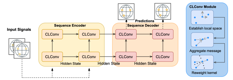
Figure 16. The framework of the CLCRN model, which is implemented based on the Sequence to Sequence architecture with the encoder fed with previously observed data and the decoder generating the predictions (Lin et al., 2022).

4.1.2. Sea surface chlorophyll-a prediction

Predicting the sea surface chlorophyll-a (Chl-a) concentration could facilitate the monitoring and early warning of harmful algal bloom events which have serious impacts on marine fisheries. For Chl-a prediction, the major difficulty is to model the seasonality and the related factors affecting Chl-a. Vollenweider (Vollenweider, 1975) et al. proposed a simple first-order equation to predict Chl-a by adjusting the parameters of the equation. ARIMA is one of the most common predictive models for predicting the Chl-a and has been applied to predict the distribution of Chl-a in the Japan Sea based on satellite data (Kiyofuji et al., 2006). Although these models are able to predict the linear dependencies in Chl-a, they do not consider other factors affecting Chl-a. Liu et al. (Liu et al., 2010) used the absolute principal components score (APCS) method to simulate the effects of multiple chemical variables on Chl-a in Lake Qilu. However, these statistical methods are of low prediction accuracy.

In recent years, various machine learning methods (e.g., neural networks, SVM, decision trees (DT), RF, feed-forward neural network (FFNN), and regression models) are widely used for Chl-a prediction (Zhang et al., 2016). For example, an FFNN model (Recknagel et al., 2002) was used to forecast the Chl-a concentration seven days in advance in the Lake Kasumigaura of Japan and obtained better performance than the statistical methods. These models can capture the complex relationship by training the parameters with past observations and achieving good performance. To further explore the ST dependencies between different ocean locations, Hill et al. (Hill et al., 2020) used a CNN to predict Chl-a concentrations within the Gulf of Mexico region and achieved better performance than traditional machine learning methods. Yossof et al. (Yussof et al., 2021) adapted an LSTM model and a CNN model to predict the harmful algal blooms on the western coast of Sabah.

To well learn the seasonality and tendency of Chl-a for long-term prediction, we need to capture the dynamic dependencies of Chl-a over time. Liu et al. (Na et al., 2022) combined the CNN-LSTM model with ST trend analyses, and increased the prediction accuracy of Chl-a in future 3 years. Wang and Xu (Wang and Xu, 2020) used a dual-stage attention-based RNN (DA-RNN) to predict Chl-a concentration. The results show that the LSTM model outperforms the CNN model in terms of prediction accuracy. Ye et al. (Ye et al., 2023) proposed the Spatiotemporal attention network predict the Chl-a with gap-filled Chl-a data and achieve high long-term accuracy. Although they are many existing methods adapting machine learning algorithms to predict Chl-a, they seldom model the relationship between Chl-a and other ocean factors (e.g., temperature and PH). Moreover, due to the difference in hydrology, climate, geochemistry, and biological characteristics of different ocean regions, existing Chl-a prediction methods may not have the transferability to be suitable for all ocean regions. In this case, how to design a general Chl-a prediction model is still an ongoing research problem.

4.1.3. Ocean surface current prediction

Ocean surface current refers to the large-scale, regular, and stable flows of water on the surface of ocean in a certain direction throughout the year. Accurate prediction of ocean currents can not only assist shipping, fishery, and tourism to produce economic benefits but also play an important role in many marine tasks such as vessel path planning and Autonomous Underwater Vehicles (AUS) controlling. The major challenge in ocean surface current prediction is to model the dynamics of slow and large-scale currents. Earlier studies on ocean current prediction mostly used numerical modeling methods such as physical models of ocean circulation and linear statistical models. For example, the physical methods calculate currents from the sea surface height with physical equations (Le Traon and Morrow, 2001; Sinha and Abernathey, 2021). As for statistical models, Frolov et al. (Frolov et al., 2012) developed an ocean surface current prediction model based on the linear autoregressive technique. Barrick et al. (Barrick et al., 2012) presented a short-term statistical system that only requires a few hours of previous data to predict future ocean surface currents in Northern Norway. Nevertheless, these physical and statistical methods require substantial processing expenses and predetermined parameters that must be manually given by domain experts.

With the development of machine learning, non-parametric prediction methods are gradually used for ocean current prediction. Many machine learning algorithms, e.g., Gaussian Processes, SVM, Genetic Algorithm, and Artificial Neural Network (ANN) have been utilized to improve the prediction accuracy of currents (Sarkar et al., 2018; Guozhen et al., 2017; Remya et al., 2012). For example, Sarkar et al. (Sarkar et al., 2019) proposed an ANN method with fully connected layers and recurrent LSTM layers to predict the tidal currents in a given region and achieved good results. Alexandre et al. (Immas et al., 2021) proposed a Transformer model with LSTM to capture the ST dependencies using real-time in-situ data to predict ocean currents. Nathachai et al. (Thongniran et al., 2019) proposed an ST model that takes advantage of noticeable domain characteristics by using a CNN to capture the spatial property and the GRU to capture the temporal property.

Although existing studies can already capture the ST information in ocean surface current data and achieve good prediction performance, the large-scale spatial dependencies and the correlations with other related factors (e.g., wind flow and the ocean tides) are still not well considered, which affect the prediction accuracy of ocean surface currents.

4.1.4. Sea ice prediction

Sea ice is simply frozen ocean water. Sea ice prediction is a crucial task to monitor and prevent global warming and also plays an important role in coastal port traffic and vessel path planning. For the study of sea ice, data from satellites are often the main or even the only data source because it is difficult to obtain in-situ sea ice observation data in extreme weather. According to (Mu et al., 2023), the ever-increasing melting speed has made it more difficult to make accurate sea ice predictions. Consequently, how to utilize the limited data to predict future sea ice data is a challenging issue.

Currently, the majority of the studies on sea ice prediction are data-driven methods (Lindsay et al., 2008). Traditional machine learning methods, e.g., BP network, ANN, and linear regression (Drobot et al., 2006), are widely used for sea ice prediction. For example. Li et al. (Li et al., 2021c) provided a sea ice-intensive degree-day prediction method that combines kernel Granger Causality analysis (KGC) and SVM to predict the sea ice. However, these machine learning methods ignore the ST dependencies in sea ice data, which leads to low prediction accuracy. To further capture the spatial dependencies, Wang et al. (Wang et al., 2016) proposed a CNN-based method to estimate the sea ice in the melting seasons by using image data from satellites. Wang et al. (Wang et al., 2017) provided the fully convolutional neural networks (FCNN) model to predict sea ice along the east coast of Canada and the model achieves high prediction accuracy. To capture the temporal dependencies in sea ice data, Petrou et al. (Petrou and Tian, 2017) used ConvLSTM to learn the temporal information and obtain good performance in short-term sea ice prediction. Chi et al. (Chi and Kim, 2017) proposed a monthly sea ice prediction model using MLP and LSTM, and achieved good performance on the arctic sea ice concentration data. To identify the impactful factors on sea ice, Mu et al. (Mu et al., 2023) proposed an interpretable long-term prediction model (IceTFT) which fuses multiple atmospheric and oceanic variables as input to train the model, and utilizes the temporal fusion transformer and the multi-head attention mechanism to automatically adjust the weights of predictors and filter spuriously correlated variables.

Most of the current studies on sea ice prediction are purely data-driven methods (Liu et al., 2021). However, it has been proven that combining physical knowledge with machine learning is an effective way to achieve accurate sea ice prediction. Currently, how to combine the physical mechanisms of sea ice with data-driven methods remains a challenging issue for achieving accurate sea ice prediction.

4.1.5. Sea tide prediction

Tides are periodic fluctuations of the ocean surface and are caused by the gravitational pull of the sun and moon. Tidal energy generated by the fluctuation of tidal water level is a vital renewable energy source (Lee and Jeng, 2002). For a long time, tide prediction provides safety guarantees for port operations, shipping traffic, and coastal protection, and also provides important support for offshore aquaculture and the prevention of natural disasters.

In the early ages, the most commonly used technique to predict sea tides is harmonic analysis which forecasts the tidal variations with historical observations. However, harmonic analysis suffers from the fact that the parameters are numerous and some of which have a very long return period, thus costing a lot of time. Currently, the widely-used methods for tidal prediction are also based on machine learning. For example, Sarkar et al. (Sarkar et al., 2016) used the BP algorithm, cascade correlation algorithm, and conjugate gradient algorithm to predict the tides continuously. Kavousi-Fard et al. (Kavousi-Fard, 2016) proposed a probabilistic method that uses Lower Upper bound Estimation (LUBE) to model the uncertainties of tidal current prediction, and achieves good prediction performance in the Bay of Fundy, NS, Canada. Granata et al. (Granata and Di Nunno, 2021; Okwuashi and Ndehedehe, 2017) used tree regression, RF, and multilayer perceptron to predict the tide level of Venice based on satellite data.

Due to the high sparsity and large spatial resolution of satellite data, it is difficult to build a high-quality unified sea tide prediction model. Meanwhile, the geology and geomorphology of the local environment are also crucial for predicting the sea tide. However, these methods above do not consider multiple source data and external factors, resulting in low prediction accuracy. To address this issue, some researchers integrate multi-source sea tide data and external factors to predict tides. For example, Yang et al. (Yang et al., 2021) integrated satellite data and tide gauge data to estimate tidal sea level using a Deep Belief Network (DBN). Riazi et al. (Riazi, 2020) built a DNN to achieve tidal level prediction by using tidal generating force, and geological and biological factors as inputs. However, the deep ST correlations in sea tide data are still not fully utilized by existing methods to improve the prediction accuracy for sea tides.

In a word, with the development of various STDM methods, ST prediction has gained a lot of attention and boosted the prediction accuracy of various ocean factors as discussed above. Further uncovering the hidden and deep ST correlations in ST ocean data and fusing them into the prediction models are still an open problem for ST prediction in ocean.

4.2. Spatial-temporal Event Detection

In ocean science, an ST event usually means that there are significant and persistent changes happening at a particular time and location, such as typhoons, eddies, and other extreme ocean phenomena. Monitoring and detecting these events can provide early warning to prevent severe damage to personal safety and social safety. In recent years, extreme ocean events become more and more frequent under the circumstance of global warming. Therefore, accurate detection and automatic identification of ST events in ocean are of significance and attract a variety of researchers. Specifically, in this section, we give a brief overview of the detection of typical ST ocean events, i.e., typhoons, eddy, and El Ni$\mathrm{\tilde{n}}$o event.

4.2.1. Typhoon detection

A typhoon refers to a large storm system that has a circular or spiral system of violent winds and typically has hundreds of kilometers in diameter. Typhoon often occurs in the tropical ocean and is usually accompanied by strong winds, heavy rain, and storm surge. Typhoon detection is of high importance to provide early warnings for disaster management in coastal areas. Typhoons usually move rapidly and are affected by multiple environmental parameters, e.g., SST, cloud cover, atmospheric pressure, and wind speed. To detect a typhoon, it is crucial to capture the extreme changes of these factors at a particular time and location. Typhoon detection has been studied for decades and existing methods can be roughly grouped into two categories, i.e., statistical-based methods and image-based methods, according to the type of data.

For the statistical-based methods, typhoon-related atmospheric and oceanic factors (e.g., SST and wind speed) and tide-gauge data are collected for the detection of typhoons. For example, Ali et al. (Ali et al., 2007) used ANNs and BP methods to achieve the 24-hour track prediction of cyclones in the Indian Ocean and the Northwest Pacific Ocean. Alemany et al. (Alemany et al., 2019) established a fully connected RNN by using typhoon center location, wind speed, and central pressure at 6-hour intervals from NOAA to reduce truncation error in classical numerical prediction methods. Sophie et al. (Giffard-Roisin et al., 2018) combined the NOAA unifying tropical cyclone data with the ERA reanalysis wind field data to construct a fusion neural network for typhoon path prediction. To predict the typhoon formation process and intensity, Chen et al. (Chen et al., 2019b) combined the CNN and LSTM to learn the spatial relationship and temporal relationship, respectively, among typhoon-related atmospheric and oceanic variables. Moreover, many researchers formulate typhoon detection as an ST clustering problem, which can not only discover the typhoon but also localize central typhoon cyclones. Kim et al. (Kim et al., 2011) evaluated the typhoon detection performance of three different clustering methods (i.e., K-means clustering, Fuzzy C-means clustering (FCM), and hierarchical clustering), and the results show that FCM is better in clustering efficiency and fitting degree. Yang et al. (Yang et al., 2017) used the mixed regression clustering algorithm and the mass moment of the typhoon cyclone trajectory method to identify the typhoon tracks in the South China Sea.

With the development of computer vision and the increasing amount of satellite image data, CNN-based methods are widely used to discover typhoons. Kovordanyi et al. (Koner, 2019) established a multi-layer ANN to predict the movement of cyclones based on the AVHRR images from NOAA. Ruttgers et al. (Ruttgers et al., 2018) proposed the GAN-based detection method and found that combining the reanalysis data of physical models and satellite image data can improve detection performance. Kim et al. (Kim et al., 2019b) proposed a ConvLSTM-based ST model to ascertain the tracks of typhoons and predict their future positions. Considering that typhoons are relatively rare weather phenomena and the proportion of positive and negative samples could be seriously unbalanced, Zhao et al. (Zhao et al., 2020) proposed a CNN-based detection method with data enhancement technology, such as shearing, rotation, and gray-level transformation, to generate new samples for better typhoon events detection.

The state-of-the-art typhoon detection methods can already achieve quite good detection performance. However, achieving real-time typhoon detection is still a challenging problem due to the high complexity of detection methods and the complex dynamics in the development of typhoons.

4.2.2. Ocean eddy identification

An eddy is a circular current of water. Ocean eddies play an important role in ocean energy transfer and nutrient distribution. Accurately identifying the variation of ocean eddies is the key to understanding the oceanic flow and ocean circulation system (Weiss, 1991). It is challenging to autonomously detect eddies since they are not static objects, but a distortion evolving through a continuous field. Images obtained from satellite sensors have a large spatial resolution and a wide swath of observation, which makes them effective sources for gaining comprehensive and detailed information to detect ocean eddies. Existing methods for ocean eddy identification can be roughly grouped into two categories, i.e., physical-based methods and data-driven methods.

The physical-based methods describe and detect the eddies with their physical information. The Okubo-Weiss method (Weiss, 1991) is the most popular statical and physical procedure to discover the patterns of eddies, and it also has good interpretability. Chelton et al. (Chelton et al., 2011) tracked and investigated the eddies’ variability globally using sixteen years of unified sea surface height data. Yang et al. (Min and Jin-song, 2013) proposed a logarithmic spiral edge fitting-based method to extract eddy information such as the center position, diameter, and edge size, from satellite images. These methods are dependent on the physical parameters, geometrics, and handcrafted features related to eddies. However, eddies are highly dynamic and the underlying physical processes are too complex to be described using the physical models with predetermined parameters.

Instead of extracting factors based on expert knowledge, data-driven models can learn high-level eddy features automatically from data. For example, Du et al. (Du et al., 2019b) utilized a spatial pyramid model and an SVM classifier method to recognize the eddies in satellite image data. As shown in Fig. 17, Wang et al. (Wang et al., 2022c) proposed the object detection method using the Data-Attention-Yolo to process the satellite data and achieved high performance on eddy identification. And Zhao et al. (Zhao et al., 2023a) developed the pyramid split attention (PSA) eddy detection U-Net architecture (PSA-EDUNet) that targets oceanic eddy identification from ocean remote sensing imagery and gain good result. These data-driven methods utilizing satellite data are proven to be effective for eddy detection. However, due to the limited resolution of satellite data, existing methods can only discover eddies with a large diameter but lack the ability to detect eddies with a diameter smaller than 50km.

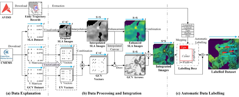
Figure 17. The framework of data-attention-YOLO for eddy identification. Here, (a) the two input datasets, (b) the data processing and integration process, and (c) automatic data labeling that is designed to transform the original eddy data to the labeled integrated data (Wang et al., 2022c).

4.2.3. El Ni${\tilde{n}}$o detection

El Ni$\mathrm{\tilde{n}}$o is an irregularly periodic variation in winds and SST over the tropical Eastern Pacific Ocean, and it can cause extreme weather events, e.g., floods and droughts, around the world. An El Ni$\mathrm{\tilde{n}}$o event can be identified if the absolute value of the 3-month mean of SST in the Ni$\mathrm{\tilde{n}}$o 3.4 region ($5^{\circ}$S-$5^{\circ}$N, $170^{\circ}$E - $120^{\circ}$W) reaches or exceeds $0.5^{\circ}C$ and lasts for at least 5 months. Since the 1970s, there are many researchers working on El Ni$\mathrm{\tilde{n}}$o detection and various models have been proposed to identify the presence of a shift into El Ni$\mathrm{\tilde{n}}$o events in advance and predict the event duration and strength to allow early preparation for the related disasters. In general, El Ni$\mathrm{\tilde{n}}$o event has mutual influence with many other regions across the world. Therefore, the biggest challenge for El Ni$\mathrm{\tilde{n}}$o detection is to capture the complex ST dependencies of the SST in different regions within a large spatial coverage.

Most early El Ni$\mathrm{\tilde{n}}$o detection models use physical laws and mathematical equations to deduce the results from the complicated interaction between the atmosphere and ocean (Kirtman, 2003). However, these methods need domain knowledge and require a lot of factor setting of functions. To address this issue, many researchers use data mining methods for El Ni$\mathrm{\tilde{n}}$o detection, which do not involve physical equations and achieve better performance than the physical type (Tang et al., 2018; Cane et al., 1986). For example. Cane et al. (Cane et al., 1986) proposed a linear dynamical model to identify the El Ni$\mathrm{\tilde{n}}$o event one year ahead.

Recently, with sufficient observational data and increasing computational power, deep learning methods are introduced to achieve long-term (e.g., more than one year) prediction and detection of El Ni$\mathrm{\tilde{n}}$o events. For instance, Wang et al. (Wang et al., 2021a) combined the ConvLSTM Encoder-Decoder model with the Empirical Mode Decomposition (EMD) technique to achieve El Ni$\mathrm{\tilde{n}}$o prediction three years in advance. Gao et al. (Gao et al., 2021) proposed a new inflation scheme based on a local ensemble transform Kalman filter to improve the long-term prediction of El Ni$\mathrm{\tilde{n}}$o events. Though these methods can provide valuable suggestions on whether El Ni$\mathrm{\tilde{n}}$o events will occur, it is still difficult to detect the onset of an El Ni$\mathrm{\tilde{n}}$o event because a series of reactions together lead to the El Ni$\mathrm{\tilde{n}}$o events. Moreover, the existing detection models do not have good interpretability, which leads to poor confidence in the results.

4.3. Spatial-temporal Pattern Mining

ST patterns mining is a fundamental task of STDM to discover the hidden, potentially useful, and unknown associations and correlations among ST ocean data. Classifying and identifying specific patterns or key features in ST ocean data are of great importance for various applications such as finding circulation regimes, discovering teleconnection patterns between weather phenomena at widely separated locations, identifying extreme-causing weather patterns, and evaluating the effects of climate changes. In this section, we will review some notable ST pattern mining approaches, i.e., clustering, EOF analysis, and correlation mining, in ocean.

4.3.1. Spatial-temporal clustering

Clustering is one key data analysis task in data mining, which aims to group the input data samples and put the samples of high similarity into one class. In general, each data sample to be classified is defined as an input vector, and the clustering result is determined by calculating the similarity between the input vector and the clustered vectors. If the similarity reaches a certain value, the input vector is divided into the corresponding classes. Compared with linear regression analysis, clustering methods (e.g., hierarchical clustering, K-means clustering, and self-organizing maps clustering) are able to reveal unknown and hidden patterns without prior knowledge from domain experts.

At an early age, hierarchical clustering methods are utilized to discover the spatial patterns of ocean circulation in the northern hemisphere (Mo and Ghil, 1988; Cheng and Wallace, 1993). Hoffman et al. (Hoffman et al., 2005) developed a quantitative statistical clustering technique termed Multivariate Spatio-Temporal Clustering (MSTC) to identify the regions with similar environmental characteristics, e.g., the dry high-altitude weather of North American and Asian winters, warming weather in Antarctica and western Greenland. White et al. (White et al., 2005) utilized the K-means method to generate the climate and vegetation clusters which were used to infer phenological responses to climate changes. Gu et al. (Gu et al., 2022) provided a hybrid estimation method that combines the k-means clustering algorithm and an ANN model to reveal the seasonal variation patterns of SST and salinity in the Indian Ocean. Moreover, Rafael et al. (Meza-Padilla et al., 2019) applied the dual SOM method to analyze the ocean salinity and currents data from 1993 to 2012 to discover the ocean circulation and its variability patterns, thus revealing the recurrent circulation patterns during different seasons. McGuire et al. (McGuire et al., 2010) developed a spatial neighborhood generation method combined with a temporal interval generation method to identify the regions with similar characteristics in SST data.

Although there are already numerous studies on ST clustering, the physical meaning, and significance of generated clusters are sometimes debatable. Moreover, there are no guarantees to find meaningful ST patterns because of the high spatial and temporal variability in ocean data. Therefore, how to develop an effective ST clustering method to produce clustering patterns with physical meanings is still a big problem for ocean science.

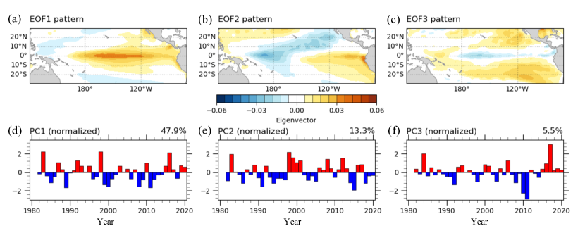
Figure 18. Spatial distributions (a,b,c) and time series (d,e,f) of the SST anomalies of the first three modes by EOF decomposition in the North Pacific Ocean from 1982 to 2020.

4.3.2. Empirical Orthogonal Function analysis

One of the most fundamental tools in ST pattern finding is Empirical Orthogonal Function (EOF) analysis. EOF is synonymous with the eigenvectors in the traditional eigenvalue decomposition of a covariance matrix (Hannachi et al., 2007). As pointed out by Cressie and Wikle (Cressie and Wikle, 2015), in the discrete case, EOF analysis is simply principle component analysis (PCA). In the continuous case, it is a Karhunen-Loeve (KL) expansion.

EOF analysis has been traditionally used to identify a low-dimensional subspace that best explains the ST variance of ocean data. In order to better understand the spatial distribution characteristics of the SST in the North Pacific, the EOF method (Jiang and Zhu, 2018) is used to analyze the variability of SST in during 1980-2020, and three spatial distributions with large variance contribution were obtained, as shown in Fig. 18. To capture clear ST patterns, researchers seek to identify dominant spatial structures and their evolution over time. For instance, Harika and Virendra (Munagapati and Tiwari, 2021) utilized EOF to identify the three broad divisions of the ocean region, i.e., western, central, and eastern, based on the seasonal ice mass gain or loss from satellite data, which corresponds to the climatic changes. Yan et al. (Prebet et al., 2019) proposed an EOF-based method to retrieve the displacement signal for decorrelating targets in satellite data.

In a word, EOF is a powerful analysis method that has been widely used in ocean science. However, in the big data era, the existing versions of EOF are slightly out of date, and there is a need to develop new EOF-related methods to take full advantage of the large amount of ST ocean data and the advanced STDM techniques.

4.3.3. Spatial-temporal correlation mining

Correlation mining in ocean aims to analyze the relationship between ocean variables, e.g., understanding ocean-atmosphere interaction, studying the effects of climate change, and finding the hidden correlations of teleconnection patterns. Various methods, including linear analysis methods and statistical decomposition methods, have been proposed for ST correlation mining in ocean. Goldenberg and Shapiro (Goldenberg and Shapiro, 1996) used linear and partial linear correlations to analyze the relationship between the vertical wind shear in the Atlantic and the SST and Sahel rainfall patterns. Webster et al. (Webster et al., 2005) analyzed the linear correlations between basin-wide mean SST and seasonal Tropical Cyclone counts in all the major basins between 1970-2005 and concluded that the upward trend in Atlantic Tropical Cyclone seasonal counts cannot be attributed to the increased SST. Chen et al. (Chen et al., 2011) used the linear regression method to discover the correlations between different oceanic regions and fire activity in Amazon from the global SST data. Hoyos et al. (Hoyos et al., 2006) used composite analysis to quantify how well one variable (e.g., SST and humidity) explains the intensity in a typhoon event. Yang et al. (Yang and Lau, 2004) utilized singular value decomposition (SVD) to discover the correlations between the summertime cloud over Central-eastern China and the warming trend of SST in the Indian Ocean. Liu et al. (Liu et al., 2012) applied linear analysis to reveal the significant correlation between the forest resources and SST over the western-north Pacific Ocean area. Liu et al. (Liu et al., 2016) adopted the SOM method to reveal the patterns of the loop current system in the eastern Gulf of Mexico.

4.4. Spatial-temporal Anomaly Detection

Anomalies refer to the sets of observations that appear to deviate from expected behavior as compared with other observations. ST anomaly detection in ocean domain is an important task and is used in a wide variety of ocean applications. For example, trajectory anomaly detection can be used to detect whether a ship is currently undertaking a voyage that may cause an accident or whether it has changed its route to avoid bad weather conditions. In this section, we summarize three typical ST anomaly detection tasks, i.e., trajectory anomaly detection, sensor time-series anomaly detection, and satellite image anomaly detection, for STDM in ocean.

4.4.1. Trajectory anomaly detection

During the voyage of the ship, various abnormal situations may be encountered, such as equipment failure, rocking and collision, and illegal activities. It is of high significance to implement effective trajectory anomaly detection, which enables timely detection and notification of abnormal events, and helps quickly take measures to protect property safety and people safety. With over 1,490,776 ships tracking worldwide (Wolsing et al., 2022), it is difficult and time-consuming to manually find anomalies. Therefore, automatically analyzing the trajectory data to quickly and accurately detect anomalies is of high necessity. To this end, many trajectory anomaly detection methods have been proposed, and these methods can be roughly divided into two categories, i.e., rule-based methods, and learning-based methods.

Rule-based methods use a set of rules for anomaly detection, which requires a good understanding of the anomalies (Kazemi et al., 2013; Soleimani et al., 2015; Riveiro and Falkman, 2009). For example, Soleimani et al. (Soleimani et al., 2015) proposed a near-optimal path method to detect ship trajectory anomalies and can also provide reasonable explanations for the detected anomalies. However, in practice, it is difficult to design a complete set of rules to cover various trajectory anomalies. Moreover, rule-based methods are often time-consuming and labor-intensive, which also limits their applications.

For learning-based methods, many researchers utilize stochastic methods and machine learning methods, e.g., the classification model (Fahn et al., 2019), gaussian process (Rong et al., 2019), gaussian mixture model (Anneken et al., 2015), density estimation model (Rong et al., 2020), and bayesian network (Forti et al., 2021), to achieve trajectory anomaly detection. For example, Fahn et al. (Fahn et al., 2019) proposed a typical classification method based on SVM and K-Nearest Neighbors (KNN) to classify ship trajectories for detecting the abnormal ones. However, classification-based detection methods require manually labeling the trajectories, and are prone to the risk of overfitting (Han et al., 2020a). To solve this problem, Han et al. (Han et al., 2021a) introduced the density-based clustering method DBSCAN to learn the distribution of trajectories without labeling and achieved good performance. Xie et al. (Xie et al., 2023) developed the Gaussian Mixture Variational Autoencoder (GMVAE) using an unsupervised classification method and achieved a high detection rate (91.26%). Martha et al.(Ferreira et al., 2022) combined autoregressive and cluster analysis to detect anomalies in maritime navigation trajectories. To further capture the hidden and deep correlations, Duong et al. (Nguyen et al., 2021) proposed GeoTrakNet which utilizes neural networks to learn the probability representation of AIS trajectories for detecting trajectory anomalies. Fig. 19 visualizes the results of three typical trajectory anomaly detection methods on the same dataset, where the GeoTrakNet achieves the best performance. Kexin et al. (Li et al., 2023) proposed an adaptive vessel trajectory anomaly detection model based on transfer learning and transformer architecture, which introduces multiple attention modules to mine the dynamic dependencies between data points in the trajectory sequence.

Although there exist many methods for trajectory anomaly detection in ocean, an objective and fair comparison between these methods is hardly possible due to closed evaluation datasets and missing ground truth for anomalies. Therefore, it is worthwhile to further explore unsupervised or semi-supervised trajectory anomaly detection methods based on the large volume of unlabeled trajectory data and limited labeled data.

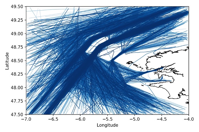
(a) All AIS tracks

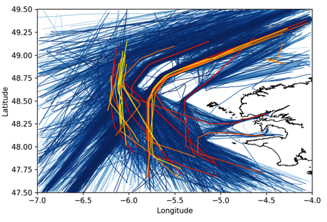
(b) LSTM

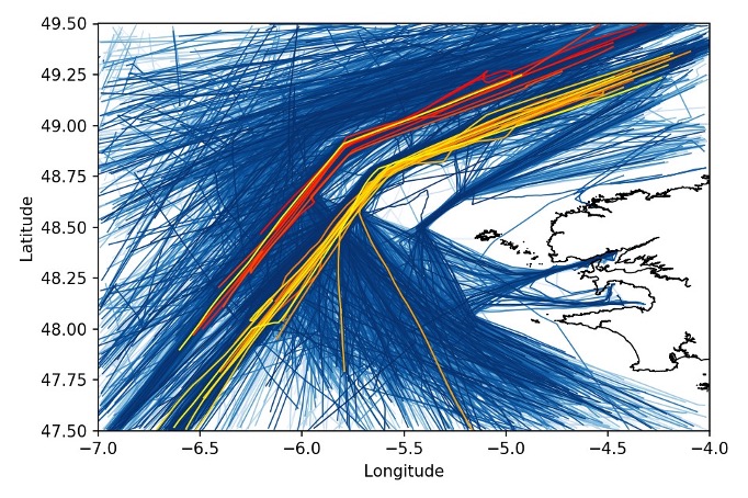
(c) DBSCAN-based

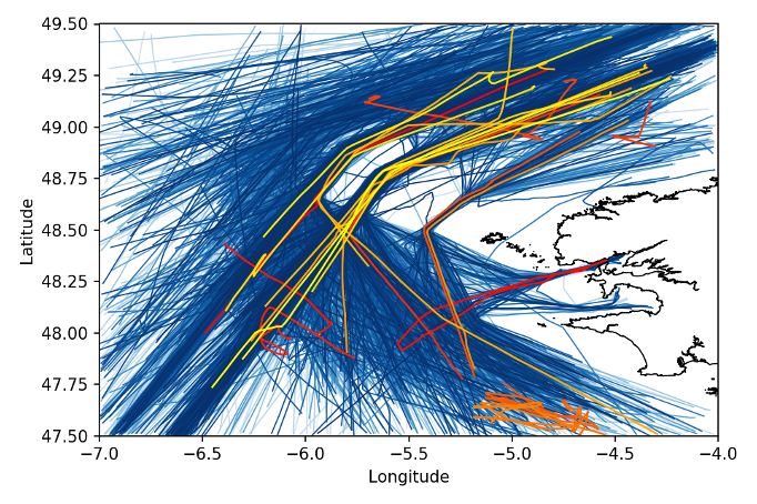
(d) GeoTrackNet

Figure 19. The visualization of AIS trajectories and the corresponding detection results of three trajectory anomaly detection methods (Nguyen et al., 2021) from January 1 to March 31, 2017, where blue color indicates normal trajectories and other colors indicate the detected abnormal trajectories.

4.4.2. Sensor time-series anomaly detection

Many in-situ sensors are usually located in harsh environmental conditions and transmit the collected data across networks. Hence, the collected data usually contain a series of outliers and anomalies. Detecting these outliers and anomalies is very important for improving the quality and reliability of the ST ocean datasets. To this end, the major difficulty is to differentiate the true anomaly rather than the regular fluctuation, which requires a good understanding of the corresponding environmental circumstances. Researchers have developed many automated statistical and machine-learning methods to jointly use spatial and temporal information for detecting sensor time-series anomalies. For example, Barua (Barua and Alhajj, 2007) used a parallel wavelet transform to detect ST outliers in SST time-series data. Kumars (Mahmoodi and Ghassemi, 2018) utilized three typical outlier detection algorithms, i.e., Box-plot (BP), Local Distance-based Outlier Factor (LDOF), and Local Outlier Factor (LOF), to detect the outliers in wave height time-series records. Anbaro (Anbaroğlu, 2009) used an ST ARIMA model to define the coherent ST neighborhoods and then detected the outliers which have their values significantly different from the mean of nearby ST neighborhoods. Wu et al. (Wu et al., 2008) detected the ST outliers in precipitation data by storing high discrepancy spatial regions over time in a tree. Ali et al. (Haj-Hassan et al., 2020) utilized a robust z-score algorithm and isolation forest to detect outliers in sensor networks, achieving good detection accuracy with a low false alarm rate. Cheng and Li (Cheng and Li, 2006) developed a multi-scale algorithm to detect abnormal coastal anomalies by evaluating the changes between ST scales. Recently, Kim et al. (Kim et al., 2021) developed an autoencoder-based unsupervised learning method to detect outliers in SST data.

4.4.3. Satellite image anomaly detection

Satellite image anomalies refer to defective remote sensing images which may contain abnormal color, color cast, and unknown objects. Satellite image anomaly detection has a broad application, e.g., ship invading detection and extreme cloud detection. Detecting image anomalies is more difficult than detecting the anomalies in trajectory data and time series data because visual features are more difficult to capture than numerical features. Marino et al. (Marino et al., 2016) proposed an incoherent dual-polarization detector to identify the anomaly of small icebergs of satellite images. Han et al. (Han et al., 2021c) proposed a spectral anomaly detection method based on dictionary optimization with sparse and low-rank constraints. The error matrix that cannot be fully expressed by the optimized spectral dictionary is defined as anomalies.

Recently, various CNN-based methods have been applied for satellite image anomaly detection due to their high capability in analyzing image data and achieved promising detection results (Wang et al., 2018, 2021b). For example, Wang et al. (Wang et al., 2018) proposed a spatial pyramid pooling net combining the multivariate Gaussian distribution to extract candidate regions of ships by regarding a ship as an abnormal ocean area. However, most satellite image anomaly detection methods still rely on the labeled images with manual expert annotations, and cannot take full advantage of the large amount of unlabeled satellite image data.

5. Future Opportunities

The progress in STDM for ocean science has made significant impacts on various ocean applications as discussed above. However, there still exist many open issues that require continuous efforts from both computer science and ocean science. In this section, we highlight some promising research directions for further advancing the techniques of ocean STDM.

Fusing physical models with data-driven models. The physical models utilize a series of functions or theories to model the physical processes within the ocean (e.g., ocean circulation and heat circulation) and are an important type of technique for various oceanic problems. In the past centuries, many classical physical ocean models, including ocean calculation models (Haidvogel and Beckmann, 1999; Dijkstra, 2005), numerical ocean models (Crowley, 1968), and physical oceanography models (Stewart, 2008), have been developed. These methods only have a small number of factors determined based on expert knowledge but achieve good performance on many oceanic tasks. Recently, data-driven models have received increasing attention and are of high ability to capture hidden information by utilizing historical data for model training (Wang et al., 2022a). Some recent studies find that it is reasonable and feasible to combine physical models with data-driven methods (Von Rueden et al., 2021), which can produce more robust and accurate models that combine the advantages of both physics models and data-driven models. Typical examples include physics-aware AI, physics-informed machine learning, and physics-guided machine learning (Karniadakis et al., 2021; Ahmad and Özönder, 2020). Taking the SST prediction task as an example, Arka et al. (Jia et al., 2021) integrate traditional physical laws (e.g., temperature density and energy conservation) and recurrent graph networks to predict SST. Compared with the traditional STDM methods, the physical-guided machine learning models can achieve high physical consistency and reduce the uncertainty of results. However, there also exist multiple obstacles, e.g., the difference in data formats, problem definitions, and model structures, to fuse physical models with data-driven models. Therefore, in the future designing a general paradigm to fuse physical models with data-driven models is an interesting research direction.

Fusing multi-source ocean datasets of different modalities. As discussed in Section 2, the ocean data used in STDM tasks usually has multiple sources, including satellite data, in-situ data, ship data, and reanalysis data, and these datasets are in different modalities. Fusing multi-source datasets can obtain comprehensive information to make STDM models achieve better performance than using a single dataset or data of a single modality. Although there are already some studies on data fusion (cf. Section 3.3), there are still many challenges in fusing multi-source datasets. First, most existing ocean STDM methods focus on fusing different data sources for the same ocean factor (e.g., SST) in single tasks (e.g., SST prediction), and cannot combine the observations of multiple factors (e.g., SST, ocean current, and Chl-a) for multiple tasks (e.g., SST prediction, current prediction, and Chl-a prediction) at the same time. Second, it is difficult to handle the heterogeneity in spatial and temporal resolutions for different datasets. Furthermore, how to fuse the image satellite data, gridded reanalysis data, and ST points data is also a challenging problem. Recently, some researchers try to use transfer learning and meta-learning methods to fuse different ocean data sources and introduce the pre-training models in computer vision and urban computing (Willard et al., 2021) to capture the features of multi-modal ocean datasets. However, the challenges mentioned above are still not well addressed and require deeper investigation in the future.

Improving the interpretability of deep STDM methods. Many STDM approaches are based on deep-learning models, e.g., CNN, RNN, and Transformer, and achieve good performance on various tasks. However, these approaches are typically regarded as black boxes with poor interpretability (Fan et al., 2021). The interpretability of STDM methods means the ability to present and explain the model behaviors in understandable forms to humans, which enables users to easily make reasonable and convincing decisions (Du et al., 2019a). For ocean science, it is of high importance to build a connection between the STDM results and the underlying physics to provide valuable advice for various ocean applications, e.g., the warning of extreme weather conditions. Although attention mechanisms have been used in some previous STDM studies for ocean science to increase the model interpretability (e.g., periodicity and local spatial dependency), how to develop more interpretable STDM methods to reveal the natural laws of the ocean remains an open problem in this field (Zhang et al., 2021).

Developing end-to-end STDM models. Currently, many STDM methods for ocean science require that the input ST ocean data are complete and of high quality. To meet such requirements, data cleaning, data completion, and data fusion are conducted over the original ST ocean data. However, these processes are time-consuming and may lead to the loss of some crucial data information. For example, in the SST prediction task, the missing rate of SST records retrieved from the satellite data may be higher than 80% for some periods and locations due to the cloud coverage (Lian et al., 2023). Existing methods for SST prediction usually utilize data completion methods (e.g., history average, optimal interpolation, and GAN-based networks) to fill in the missing values before conducting the prediction. However, these methods ignore the sparse distribution of original data and the reasons behind the sparsity (e.g., typhoons and heavy rainfall), which seriously damages the prediction accuracy. Therefore, developing end-to-end STDM models to learn knowledge and patterns directly from the original sparse ST ocean data is a promising direction.

Designing large models for ocean science. Recently, the large models (e.g., BERT (Devlin et al., 2018), GPT (Floridi and Chiriatti, 2020), and ViT (Ranftl et al., 2021)) have received tremendous popularity in computer science, and surpassed many state-of-the-art machine learning models by pre-training on big datasets and fine-tuning for different downstream tasks. In ocean science, large ST ocean datasets of wide spatial coverage have been utilized to train STDM models for various oceanic tasks, which lays the solid foundation for designing unified large models. For example, a recent big weather forecasting model (i.e., Pangu-Weather (Bi et al., 2023)) is trained on 39-year global weather datasets and achieves great performance on various downstream tasks such as medium-range weather forecasting, extreme weather forecasting, and ensemble weather forecasting. In fact, pre-training models trained on large ST ocean datasets can capture the underlying patterns and regularity more effectively and produce more accurate analyzing results for various oceanic tasks. Therefore, designing large models in the domain of ocean science is of high necessity to address the heterogeneity issues in data and tasks.

6. Conclusion

The increasing numbers of satellites, buoys, and other ocean observation facilities have generated a flood of ST ocean data, which makes it possible to develop STDM methods for various ocean applications, e.g., weather forecasting and typhoon detection. The past decades have witnessed the rapid development of STDM techniques for ocean science, which enable us to uncover the underlying ST dependencies within ocean data for solving the challenging problems in ocean science. This survey provides a comprehensive overview of the existing ocean STDM studies, including the publically available ST ocean datasets and their unique characteristics as well as the data visualization tools, the data quality enhancement methods, and the methodologies for different types of STDM tasks. In addition, some promising research opportunities for future research are also pinpointed. We hope that this paper can help computer scientists identify important research issues of ocean big data, and inspire researchers in ocean science to apply advanced STDM techniques to a variety of ocean applications.

References

- (1)
- Pic (2018) 2018. Argo Floats to Improve Our Knowledge of the Ocean. https://www.euro-argo.eu/Outreach/Educational-material/Discover-Argo-floats/How-do-the-Argo-floats-fulfill-their-mission-in-the-Ocean, Last accessed on 2018-10-25.
- Pic (2020) 2020. ArcGIS Pro. https://www.esriuk.com/en-gb/arcgis/, Last accessed on 2020-8-11.
- Pic (2021a) 2021a. AVHRR. https://www.eumetsat.int/avhrr, Last accessed on 2021-10-03.
- Pic (2021b) 2021b. MODIS. https://modis.gsfc.nasa.gov/gallery/, Last accessed on 2021-10-03.
- Pic (2023a) 2023a. The visualization of trajectories of automatic identification system. https://www.marinetraffic.com/research/dataset/marinetraffic-automatic-identification-system-ais/, Last accessed on 2023-1-25.
- Pic (2023b) 2023b. The workflow of Argo sensors. https://globalocean.noaa.gov/research/argo-program/, Last accessed on 2023-1-2.
- Acharya et al. (2017) Tri Dev Acharya, Kyung Wan Yoo, and Dong Ha Lee. 2017. GIS-based Spatio-temporal Analysis of Marine Accidents Database in the Coastal Zone of Korea. Journal of Coastal Research 79, sp1 (2017), 114 – 118.
- Aguilar-Martinez and Hsieh (2009) Silvestre Aguilar-Martinez and William W. Hsieh. 2009. Forecasts of Tropical Pacific Sea Surface Temperatures by Neural Networks and Support Vector Regression. International Journal of Oceanography (2009), 1–13.
- Ahmad and Özönder (2020) Muhammad Aurangzeb Ahmad and Şener Özönder. 2020. Physics inspired models in artificial intelligence. In Proceedings of the 26th ACM SIGKDD International Conference on Knowledge Discovery & Data Mining. 3535–3536.
- Alemany et al. (2019) Sheila Alemany, Jonathan Beltran, Adrian Perez, and Sam Ganzfried. 2019. Predicting hurricane trajectories using a recurrent neural network. In Proceedings of the AAAI Conference on Artificial Intelligence, Vol. 33. 468–475.
- Ali et al. (2007) MM Ali, CM Kishtawal, and Sarika Jain. 2007. Predicting cyclone tracks in the north Indian Ocean: An artificial neural network approach. Geophysical research letters 34, 4 (2007).
- Alvera-Azcárate et al. (2007) A. Alvera-Azcárate, A. Barth, J.-M. Beckers, and R. H. Weisberg. 2007. Multivariate Reconstruction of Missing Data in Sea Surface Temperature, Chlorophyll, and Wind Satellite Fields. Journal of Geophysical Research 112, C3 (2007).
- Alvera-Azcárate et al. (2005) Aïda Alvera-Azcárate, Alexander Barth, Michel Rixen, and Jean-Marie Beckers. 2005. Reconstruction of incomplete oceanographic data sets using empirical orthogonal functions: application to the Adriatic Sea surface temperature. Ocean Modelling 9, 4 (2005), 325–346.
- Anbaroğlu (2009) Tao Cheng Berk Anbaroğlu. 2009. Spatio-temporal outlier detection in environmental data. Spatial and Temporal Reasoning for Ambient Intelligence Systems (2009), 1–10.
- Anneken et al. (2015) Mathias Anneken, Yvonne Fischer, and Jürgen Beyerer. 2015. Evaluation and comparison of anomaly detection algorithms in annotated datasets from the maritime domain. In 2015 SAI Intelligent Systems Conference (IntelliSys). IEEE, 169–178.
- Aouf et al. (2018) Lotfi Aouf, Danièle Hauser, Celine Tison, and Bertrand Chapron. 2018. On the Assimilation of Multi-Source of Directional Wave Spectra from Sentinel-1A and 1B, and CFOSAT in the Wave Model MFWAM: Toward an Operational Use in CMEMS-MFC. In 2018 IEEE International Geoscience and Remote Sensing Symposium, IGARSS 2018, Valencia, Spain, July 22-27, 2018. IEEE, 5663–5666.
- Baik and Paek (2000) Jong-Jin Baik and Jong-Su Paek. 2000. A neural network model for predicting typhoon intensity. Journal of the Meteorological Society of Japan. Ser. II 78, 6 (2000), 857–869.
- Banks et al. (2012) Christopher J. Banks, Christine Gommenginger, Meric Srokosz, and Helen M. Snaith. 2012. Validating SMOS Ocean Surface Salinity in the Atlantic With Argo and Operational Ocean Model Data. IEEE Trans. Geosci. Remote. Sens. 50, 5-1 (2012), 1688–1702.
- Barrick et al. (2012) Donald Barrick, Vicente Fernandez, Maria I Ferrer, Chad Whelan, and Øyvind Breivik. 2012. A short-term predictive system for surface currents from a rapidly deployed coastal HF radar network. Ocean Dynamics 62 (2012), 725–740.
- Barth et al. (2020) Alexander Barth, Aida Alvera-Azcárate, Matjaz Licer, and Jean-Marie Beckers. 2020. DINCAE 1.0: A Convolutional Neural Network with Error Estimates to Reconstruct Sea Surface Temperature Satellite Observations. Geoscientific Model Development 13, 3 (2020), 1609–1622.
- Bartier and Keller (1996) Patrick M Bartier and C Peter Keller. 1996. Multivariate interpolation to incorporate thematic surface data using inverse distance weighting (IDW). Computers & Geosciences 22, 7 (1996), 795–799.
- Barua and Alhajj (2007) Sajib Barua and Reda Alhajj. 2007. Parallel wavelet transform for spatio-temporal outlier detection in large meteorological data. In Intelligent Data Engineering and Automated Learning-IDEAL 2007: 8th International Conference, Birmingham, UK, December 16-19, 2007. Proceedings 8. Springer, 684–694.
- Beckers and Rixen (2003) J. M. Beckers and M. Rixen. 2003. EOF Calculations and Data Filling from Incomplete Oceanographic Datasets*. Journal of Atmospheric and Oceanic Technology 20, 12 (2003), 1839–1856.
- Bhaskar and Jayaram (2015) Tata V. S. Udaya Bhaskar and Chiranjivi Jayaram. 2015. Evaluation of Aquarius Sea Surface Salinity With Argo Sea Surface Salinity in the Tropical Indian Ocean. IEEE Geosci. Remote. Sens. Lett. 12, 6 (2015), 1292–1296.
- Bhattacharjee et al. (2014) Shrutilipi Bhattacharjee, Pabitra Mitra, and Soumya K. Ghosh. 2014. Spatial Interpolation to Predict Missing Attributes in GIS Using Semantic Kriging. IEEE Transactions on Geoscience and Remote Sensing 52, 8 (2014), 4771–4780.
- Bi et al. (2023) Kaifeng Bi, Lingxi Xie, Hengheng Zhang, Xin Chen, Xiaotao Gu, and Qi Tian. 2023. Accurate medium-range global weather forecasting with 3D neural networks. Nature (2023), 1–6.
- Binh et al. (2022) Nguyen An Binh, Pham Viet Hoa, Giang Thi Phuong Thao, Ho Dinh Duan, and Phan Minh Thu. 2022. Evaluation of Chlorophyll-a estimation using Sentinel 3 based on various algorithms in southern coastal Vietnam. Int. J. Appl. Earth Obs. Geoinformation 112 (2022), 102951.
- Boy et al. (2022) François Boy, Jean-François Crétaux, Malik Boussaroque, and Céline Tison. 2022. Improving Sentinel-3 SAR Mode Processing Over Lake Using Numerical Simulations. IEEE Trans. Geosci. Remote. Sens. 60 (2022), 1–18.
- Boyer et al. (2013) Timothy P Boyer, John I Antonov, Olga K Baranova, Hernan E Garcia, Daphne R Johnson, Alexey V Mishonov, Todd D O’Brien, Dan Seidov, Igor Smolyar, Melissa M Zweng, et al. 2013. World ocean database 2013. (2013).
- Brandoli et al. (2022) Bruno Brandoli, Alessandra Raffaetà, Marta Simeoni, Pedram Adibi, Fateha Khanam Bappee, Fabio Pranovi, Giulia Rovinelli, Elisabetta Russo, Claudio Silvestri, Amílcar Soares, and Stan Matwin. 2022. From multiple aspect trajectories to predictive analysis: a case study on fishing vessels in the Northern Adriatic sea. GeoInformatica 26, 4 (2022), 551–579.
- Buongiorno Nardelli et al. (2013) B. Buongiorno Nardelli, C. Tronconi, A. Pisano, and R. Santoleri. 2013. High and Ultra-High resolution processing of satellite Sea Surface Temperature data over Southern European Seas in the framework of MyOcean project. Remote Sensing of Environment 129 (2013), 1–16.
- Cai et al. (2019) Wen-Yu Cai, Zi-Qiang Liu, and Mei-Yan Zhang. 2019. Trajectory Clustering Based Oceanic Anomaly Detection Using Argo Profile Floats. In Communications and Networking - 14th EAI International Conference, ChinaCom 2019, Shanghai, China, November 29 - December 1, 2019, Proceedings, Part I (Lecture Notes of the Institute for Computer Sciences, Social Informatics and Telecommunications Engineering, Vol. 312). Springer, 498–508.
- Cane et al. (1986) Mark A Cane, Stephen E Zebiak, and Sean C Dolan. 1986. Experimental forecasts of EL Nino. Nature 321, 6073 (1986), 827–832.
- Chamberlain et al. (2023) Paul Chamberlain, Bruce Cornuelle, Lynne D. Talley, Kevin Speer, Cathrine Hancock, and Stephen Riser. 2023. Acoustic Float Tracking with the Kalman Smoother. Journal of Atmospheric and Oceanic Technology 40, 1 (2023), 15–35.
- Chelton et al. (2011) Dudley B. Chelton, Michael G. Schlax, and Roger M. Samelson. 2011. Global observations of nonlinear mesoscale eddies. Progress in Oceanography 91, 2 (2011), 167–216.
- Chen et al. (2022) Jianqiang Chen, Xun Gong, Xinyu Guo, Xiaogang Xing, Keyu Lu, Huiwang Gao, and Xiang Gong. 2022. Improved Perceptron of Subsurface Chlorophyll Maxima by a Deep Neural Network: A Case Study with BGC-Argo Float Data in the Northwestern Pacific Ocean. Remote. Sens. 14, 3 (2022), 632.
- Chen et al. (2019b) Rui Chen, Xiang Wang, Weimin Zhang, Xiaoyu Zhu, Aiping Li, and Chao Yang. 2019b. A hybrid CNN-LSTM model for typhoon formation forecasting. GeoInformatica 23 (2019), 375–396.
- Chen et al. (2019a) Shuangling Chen, Chuanmin Hu, Brian B. Barnes, Yuyuan Xie, Gong Lin, and Zhongfeng Qiu. 2019a. Improving Ocean Color Data Coverage through Machine Learning. Remote Sensing of Environment 222 (2019), 286–302.
- Chen and Gao (2013) Wei Chen and Bo-Cai Gao. 2013. A Multispectral Decomposition Technique for the Recovery of True SeaWiFS Top-of-Atmosphere Radiances. IEEE Geosci. Remote. Sens. Lett. 10, 2 (2013), 288–292.
- Chen et al. (2011) Yang Chen, James T. Randerson, Douglas C. Morton, Ruth S. DeFries, G. James Collatz, Prasad S. Kasibhatla, Louis Giglio, Yufang Jin, and Miriam E. Marlier. 2011. Forecasting Fire Season Severity in South America Using Sea Surface Temperature Anomalies. Science 334, 6057 (2011), 787–791.
- Chen et al. (2020) Zhuomin Chen, Young-Oh Kwon, Ke Chen, Paula Fratantoni, Glen Gawarkiewicz, and Terrence M Joyce. 2020. Long-term SST variability on the Northwest Atlantic continental shelf and slope. Geophysical Research Letters 47, 1 (2020), e2019GL085455.
- Cheng and Li (2006) Tao Cheng and Zhilin Li. 2006. A multiscale approach for spatio-temporal outlier detection. Transactions in GIS 10, 2 (2006), 253–263.
- Cheng and Wallace (1993) Xinhua Cheng and John M Wallace. 1993. Cluster analysis of the Northern Hemisphere wintertime 500-hPa height field: Spatial patterns. Journal of atmospheric sciences 50, 16 (1993), 2674–2696.
- Chi and Kim (2017) Junhwa Chi and Hyun-choel Kim. 2017. Prediction of arctic sea ice concentration using a fully data driven deep neural network. Remote Sensing 9, 12 (2017), 1305.
- Chu et al. (2012) Hone-Jay Chu, Churn-Jung Liau, Chao-Hung Lin, and Bo-Song Su. 2012. Integration of fuzzy cluster analysis and kernel density estimation for tracking typhoon trajectories in the Taiwan region. Expert Systems with Applications 39, 10 (2012), 9451–9457.
- Cowtan and Way (2014) Kevin Cowtan and Robert G Way. 2014. Coverage bias in the HadCRUT4 temperature series and its impact on recent temperature trends. Quarterly Journal of the Royal Meteorological Society 140, 683 (2014), 1935–1944.
- Cressie and Wikle (2015) Noel Cressie and Christopher K Wikle. 2015. Statistics for spatio-temporal data. John Wiley & Sons.
- Cressie (1996) Noel A Cressie. 1996. Change of support and the modifiable areal unit problem. (1996).
- Crowley (1968) WP Crowley. 1968. A global numerical ocean model: Part I. J. Comput. Phys. 3, 1 (1968), 111–147.
- Dasu and Loh (2012) Tamraparni Dasu and Ji Meng Loh. 2012. Statistical Distortion: Consequences of Data Cleaning. Proceedings of the VLDB Endowment 5, 11 (2012).
- Devlin et al. (2018) Jacob Devlin, Ming-Wei Chang, Kenton Lee, and Kristina Toutanova. 2018. Bert: Pre-training of deep bidirectional transformers for language understanding. arXiv preprint arXiv:1810.04805 (2018).
- Dijkstra (2005) Henk A Dijkstra. 2005. Nonlinear physical oceanography: a dynamical systems approach to the large scale ocean circulation and El Niño. Vol. 532. Springer.
- Dong et al. (2023) Zizhen Dong, Ruowen Yang, Jie Cao, and Lin Wang. 2023. Effect of Anthropogenic Forcing on Increased Winter Precipitation in Southeast Asia from 1979 to 2014. Frontiers in Environmental Science 10 (2023), 2723.
- Drobot et al. (2006) Sheldon D Drobot, James A Maslanik, and Charles Fowler. 2006. A long-range forecast of Arctic summer sea-ice minimum extent. Geophysical Research Letters 33, 10 (2006).
- Du et al. (2020) Mei Du, Yijun Hou, Po Hu, and Kai Wang. 2020. Effects of typhoon paths on storm surge and coastal inundation in the Pearl River Estuary, China. Remote Sensing 12, 11 (2020), 1851.
- Du et al. (2019a) Mengnan Du, Ninghao Liu, and Xia Hu. 2019a. Techniques for interpretable machine learning. Commun. ACM 63, 1 (2019), 68–77.
- Du et al. (2019b) Yanling Du, Wei Song, Qi He, Dongmei Huang, Antonio Liotta, and Chen Su. 2019b. Deep learning with multi-scale feature fusion in remote sensing for automatic oceanic eddy detection. Information Fusion 49 (2019), 89–99.
- Duan et al. (2009) Lian Duan, Lida Xu, Ying Liu, and Jun Lee. 2009. Cluster-based outlier detection. Annals of Operations Research 168 (2009), 151–168.
- Efron and Tibshirani (1991) Bradley Efron and Robert Tibshirani. 1991. Statistical Data Analysis in the Computer Age. Science 253, 5018 (1991), 390–395.
- Elman (1990) Jeffrey L Elman. 1990. Finding structure in time. Cognitive science 14, 2 (1990), 179–211.
- Elvidge et al. (2022) Christopher D. Elvidge, Tilottama Ghosh, Feng-Chi Hsu, and Mikhail N. Zhizhin. 2022. VIIRS Monitoring and Reporting on Lit Fishing Vessel Detections in Southeast Asia. In IEEE International Geoscience and Remote Sensing Symposium, IGARSS 2022, Kuala Lumpur, Malaysia, July 17-22, 2022. IEEE, 4779–4782.
- Faghmous and Kumar (2014) James H. Faghmous and Vipin Kumar. 2014. Spatio-Temporal Data Mining for Climate Data: Advances, Challenges, and Opportunities. In Data Mining and Knowledge Discovery for Big Data. Vol. 1. Springer Berlin Heidelberg, Berlin, Heidelberg, 83–116.
- Fahn et al. (2019) C Fahn, Jer Ling, M Yeh, P Huang, and M Wu. 2019. Abnormal maritime activity detection in satellite image sequences using trajectory features. International Journal of Future Computer and Communication 8, 1 (2019), 29–33.
- Fan et al. (2021) Feng-Lei Fan, Jinjun Xiong, Mengzhou Li, and Ge Wang. 2021. On interpretability of artificial neural networks: A survey. IEEE Transactions on Radiation and Plasma Medical Sciences 5, 6 (2021), 741–760.
- Fernández-Beltran et al. (2022) Rubén Fernández-Beltran, Damian Ibañez, Jian Kang, and Filiberto Pla. 2022. Time-Resolved Sentinel-3 Vegetation Indices Via Inter-Sensor 3-D Convolutional Regression Networks. IEEE Geosci. Remote. Sens. Lett. 19 (2022), 1–5.
- Ferreira et al. (2022) Martha Dais Ferreira, Jessica NA Campbell, and Stan Matwin. 2022. A novel machine learning approach to analyzing geospatial vessel patterns using AIS data. GIScience & Remote Sensing 59, 1 (2022), 1473–1490.
- Floridi and Chiriatti (2020) Luciano Floridi and Massimo Chiriatti. 2020. GPT-3: Its nature, scope, limits, and consequences. Minds and Machines 30 (2020), 681–694.
- Forti et al. (2021) Nicola Forti, Leonardo M Millefiori, Paolo Braca, and Peter Willett. 2021. Bayesian filtering for dynamic anomaly detection and tracking. IEEE Trans. Aerospace Electron. Systems 58, 3 (2021), 1528–1544.
- Frolov et al. (2012) Sergey Frolov, Jeffrey Paduan, Michael Cook, and James Bellingham. 2012. Improved statistical prediction of surface currents based on historic HF-radar observations. Ocean Dynamics 62 (2012), 1111–1122.
- Galotto-Tébar et al. (2022) M. M. Galotto-Tébar, A. Pomares-Padilla, I. A. Czerwinski, and J. C. Gutiérrez-Estrada. 2022. Is the vessel fishing? Discrimination of fishing activity with low-cost intelligent mobile devices through traditional and heuristic approaches. Expert Syst. Appl. 200 (2022), 117091.
- Gao et al. (2021) Yanqiu Gao, Youmin Tang, Xunshu Song, and Zheqi Shen. 2021. Parameter Estimation Based on a Local Ensemble Transform Kalman Filter Applied to El Niño–Southern Oscillation Ensemble Prediction. Remote Sensing 13, 19 (2021), 3923.
- Gbagir and Colpaert (2020) Augustine-Moses Gaavwase Gbagir and Alfred Colpaert. 2020. Assessing the Trend of the Trophic State of Lake Ladoga Based on Multi-Year (1997-2019) CMEMS GlobColour-Merged CHL-OC5 Satellite Observations. Sensors 20, 23 (2020), 6881.
- George et al. (2014) Richard L. S. F. George, Peter E. Robins, Alan G. Davies, Panagiotis D. Ritsos, and Jonathan C. Roberts. 2014. Interactive Visual Analytics of Hydrodynamic Flux for the Coastal Zone. Environmental Earth Sciences 72, 10 (2014), 3753–3766.
- Giffard-Roisin et al. (2018) Sophie Giffard-Roisin, Mo Yang, Guillaume Charpiat, Balázs Kégl, and Claire Monteleoni. 2018. Fused deep learning for hurricane track forecast from reanalysis data. In Climate Informatics Workshop Proceedings 2018.
- Goldenberg and Shapiro (1996) Stanley Goldenberg and Lloyd Shapiro. 1996. Physical Mechanisms for the Association of El Nino and West African Rainfall with Atlantic Major Hurricane Activity. Journal of Climate - J CLIMATE 9 (06 1996), 1169–1187.
- Granata and Di Nunno (2021) Francesco Granata and Fabio Di Nunno. 2021. Artificial Intelligence models for prediction of the tide level in Venice. Stochastic Environmental Research and Risk Assessment 35, 12 (2021), 2537–2548.
- Gu et al. (2022) Chen Gu, Jifeng Qi, Yizhi Zhao, Wenming Yin, and Shanliang Zhu. 2022. Estimation of the Mixed Layer Depth in the Indian Ocean from Surface Parameters: A Clustering-Neural Network Method. Sensors 22, 15 (2022), 5600.
- Guan et al. (2021) Yanan Guan, Jie Zhang, Xi Zhang, Zhongwei Li, Junmin Meng, Genwang Liu, Meng Bao, and Chenghui Cao. 2021. Identification of Fishing Vessel Types and Analysis of Seasonal Activities in the Northern South China Sea Based on AIS Data: A Case Study of 2018. Remote. Sens. 13, 10 (2021), 1952.
- Guo et al. (2022) Junting Guo, Jingfang Lu, Yuming Zhang, Chen Zhou, Shufang Zhang, Daosheng Wang, and Xianqing Lv. 2022. Variability of Chlorophyll-a and Secchi Disk Depth (1997–2019) in the Bohai Sea Based on Monthly Cloud-Free Satellite Data Reconstructions. Remote Sensing 14, 3 (2022), 639.
- Guozhen et al. (2017) Yang Guozhen, Wang Haifeng, Qian Hui, and Fang Jianming. 2017. Tidal current short-term prediction based on support vector regression. In IOP Conference Series: Materials Science and Engineering, Vol. 199. IOP Publishing, 012024.
- Haghbin et al. (2021) Masoud Haghbin, Ahmad Sharafati, Davide Motta, Nadhir Al-Ansari, and Mohamadreza Hosseinian Moghadam Noghani. 2021. Applications of Soft Computing Models for Predicting Sea Surface Temperature: A Comprehensive Review and Assessment. Progress in Earth and Planetary Science 8, 1 (2021), 4.
- Haidvogel and Beckmann (1999) Dale B Haidvogel and Aike Beckmann. 1999. Numerical ocean circulation modeling. World Scientific.
- Haj-Hassan et al. (2020) Ali Haj-Hassan, Carol Habib, and Jad Nassar. 2020. Real-time Spatio-Temporal based Outlier Detection Framework for Wireless Body Sensor Networks. In 2020 IEEE International Conference on Advanced Networks and Telecommunications Systems (ANTS). 1–6.
- Hamdi et al. (2022) Ali Hamdi, Khaled Shaban, Abdelkarim Erradi, Amr Mohamed, Shakila Khan Rumi, and Flora D Salim. 2022. Spatiotemporal data mining: a survey on challenges and open problems. Artificial Intelligence Review (2022), 1–48.
- Han et al. (2020a) X Han, C Armenakis, and M Jadidi. 2020a. DBSCAN optimization for improving marine trajectory clustering and anomaly detection. International Archives of the Photogrammetry, Remote Sensing & Spatial Information Sciences 43 (2020).
- Han et al. (2021a) Xuyang Han, Costas Armenakis, and Mojgan Jadidi. 2021a. Modeling vessel behaviours by clustering ais data using optimized dbscan. Sustainability 13, 15 (2021), 8162.
- Han et al. (2021c) Xiaolin Han, Huan Zhang, and Weidong Sun. 2021c. Spectral anomaly detection based on dictionary learning for sea surfaces. IEEE Geoscience and Remote Sensing Letters 19 (2021), 1–5.
- Han et al. (2021b) Yanling Han, Yekun Liu, Zhonghua Hong, Yun Zhang, Shuhu Yang, and Jing Wang. 2021b. Sea ice image classification based on heterogeneous data fusion and deep learning. Remote Sensing 13, 4 (2021), 592.
- Han et al. (2020b) Zhaohui Han, Yijun He, Guoqiang Liu, and William Perrie. 2020b. Application of DINCAE to Reconstruct the Gaps in Chlorophyll-a Satellite Observations in the South China Sea and West Philippine Sea. Remote Sensing 12, 3 (2020), 480.
- Hannachi et al. (2007) Abdel Hannachi, Ian T Jolliffe, and David B Stephenson. 2007. Empirical orthogonal functions and related techniques in atmospheric science: A review. International Journal of Climatology: A Journal of the Royal Meteorological Society 27, 9 (2007), 1119–1152.
- Hausfather et al. (2017) Zeke Hausfather, Kevin Cowtan, David C Clarke, Peter Jacobs, Mark Richardson, and Robert Rohde. 2017. Assessing recent warming using instrumentally homogeneous sea surface temperature records. Science advances 3, 1 (2017), e1601207.
- He et al. (2003) Ruoying He, Robert H. Weisberg, Haiying Zhang, Frank E. Muller-Karger, and Robert W. Helber. 2003. A Cloud-Free, Satellite-Derived, Sea Surface Temperature Analysis for the West Florida Shelf: SEA SURFACE TEMPERATURE ANALYSIS. Geophysical Research Letters 30, 15 (2003).
- Hill et al. (2020) Paul R. Hill, Anurag Kumar, Marouane Temimi, and David R. Bull. 2020. HABNet: Machine Learning, Remote Sensing-Based Detection of Harmful Algal Blooms. IEEE Journal of Selected Topics in Applied Earth Observations and Remote Sensing 13 (2020), 3229–3239.
- Hoffman et al. (2005) Forrest M Hoffman, William W Hargrove Jr, David J Erickson III, and Robert J Oglesby. 2005. Using clustered climate regimes to analyze and compare predictions from fully coupled general circulation models. Earth Interactions 9, 10 (2005), 1–27.
- Hollt et al. (2014) Thomas Hollt, Ahmed Magdy, Peng Zhan, Guoning Chen, Ganesh Gopalakrishnan, Ibrahim Hoteit, Charles D. Hansen, and Markus Hadwiger. 2014. Ovis: A Framework for Visual Analysisof Ocean Forecast Ensembles. IEEE Transactions on Visualization and Computer Graphics 20, 8 (2014), 1114–1126.
- Hosoda and Sakaida (2016) Kohtaro Hosoda and Futoki Sakaida. 2016. Global Daily High-Resolution Satellite-Based Foundation Sea Surface Temperature Dataset: Development and Validation against Two Definitions of Foundation SST. Remote Sensing 8, 11 (2016), 962.
- Hou et al. (2021) Siyun Hou, Wengen Li, Tianying Liu, Shuigeng Zhou, Jihong Guan, Rufu Qin, and Zhenfeng Wang. 2021. D2CL: A Dense Dilated Convolutional LSTM Model for Sea Surface Temperature Prediction. IEEE Journal of Selected Topics in Applied Earth Observations and Remote Sensing (2021), 12514–12523.
- Hou et al. (2022) Siyun Hou, Wengen Li, Tianying Liu, Shuigeng Zhou, Jihong Guan, Rufu Qin, and Zhenfeng Wang. 2022. MUST: A Multi-source Spatio-Temporal data fusion Model for short-term sea surface temperature prediction. Ocean Engineering 259 (2022), 111932.
- Hoyos et al. (2006) C. D. Hoyos, P. A. Agudelo, P. J. Webster, and J. A. Curry. 2006. Deconvolution of the Factors Contributing to the Increase in Global Hurricane Intensity. Science 312, 5770 (2006), 94–97.
- Hu et al. (2021) Chuanmin Hu, Lian Feng, and Qi Guan. 2021. A Machine Learning Approach to Estimate Surface Chlorophyll a Concentrations in Global Oceans From Satellite Measurements. IEEE Transactions on Geoscience and Remote Sensing 59, 6 (2021), 4590–4607.
- Hu et al. (2023) Qiwei Hu, Xiaoyan Chen, Yan Bai, Xianqiang He, Teng Li, and Delu Pan. 2023. Reconstruction of 3-D Ocean Chlorophyll a Structure in the Northern Indian Ocean Using Satellite and BGC-Argo Data. IEEE Trans. Geosci. Remote. Sens. 61 (2023), 1–13.
- Huang et al. (2021b) Boyin Huang, Chunying Liu, Viva Banzon, Eric Freeman, Garrett Graham, Bill Hankins, Tom Smith, and Huai-Min Zhang. 2021b. Improvements of the Daily Optimum Interpolation Sea Surface Temperature (DOISST) Version 2.1. Journal of Climate 34, 8 (2021), 2923–2939.
- Huang et al. (2021a) Huang Huang, Lewis R Blake, Matthias Katzfuss, and Dorit M Hammerling. 2021a. Nonstationary Spatial Modeling of Massive Global Satellite Data. arXiv preprint arXiv:2111.13428 (2021).
- Huang et al. (2021c) Jie Huang, Fengwei Zhu, Zejun Huang, Jian Wan, and Yongjian Ren. 2021c. Research on Real-Time Anomaly Detection of Fishing Vessels in a Marine Edge Computing Environment. Mob. Inf. Syst. 2021 (2021), 5598988:1–5598988:15.
- Huang et al. (2020) Mingfeng Huang, Kuan Zhang, Zhiwen Zeng, Tian Wang, and Yuxin Liu. 2020. An AUV-Assisted Data Gathering Scheme Based on Clustering and Matrix Completion for Smart Ocean. IEEE Internet of Things Journal 7, 10 (2020), 9904–9918.
- Huber et al. (2023) Manuel Huber, Craig Donlon, and Montserrat Pinol Sole. 2023. Global Surface Water Density Masks to Refine Sentinel 3 Data Acquisitions. IEEE Geosci. Remote. Sens. Lett. 20 (2023), 1–5.
- Hussein et al. (2021) Khalid A Hussein, Khameis Al Abdouli, Dawit T Ghebreyesus, Pakorn Petchprayoon, Naeema Al Hosani, and Hatim O. Sharif. 2021. Spatiotemporal variability of chlorophyll-a and sea surface temperature, and their relationship with bathymetry over the coasts of UAE. Remote Sensing 13, 13 (2021), 2447.
- Immas et al. (2021) Alexandre Immas, Ninh Do, and Mohammad-Reza Alam. 2021. Real-time in situ prediction of ocean currents. Ocean Engineering 228 (2021), 108922.
- Jahanbakht et al. (2022) Mohammad Jahanbakht, Wei Xiang, and Mostafa Rahimi Azghadi. 2022. Sea Surface Temperature Forecasting With Ensemble of Stacked Deep Neural Networks. IEEE Geosci. Remote. Sens. Lett. 19 (2022), 1–5.
- Jamet et al. (2012) Cédric Jamet, Hubert Loisel, and D Dessailly. 2012. Retrieval of the spectral diffuse attenuation coefficient Kd () in open and coastal ocean waters using a neural network inversion. Journal of Geophysical Research: Oceans 117, C10 (2012).
- Jia et al. (2021) Xiaowei Jia, Jacob Zwart, Jeffrey Sadler, Alison Appling, Samantha Oliver, Steven Markstrom, Jared Willard, Shaoming Xu, Michael Steinbach, Jordan Read, et al. 2021. Physics-guided recurrent graph model for predicting flow and temperature in river networks. In Proceedings of the 2021 SIAM International Conference on Data Mining (SDM). SIAM, 612–620.
- Jiang et al. (2019) Li-Qing Jiang, Brendan R Carter, Richard A Feely, Siv K Lauvset, and Are Olsen. 2019. Surface ocean pH and buffer capacity: past, present and future. Scientific reports 9, 1 (2019), 18624.
- Jiang and Zhu (2018) Ning Jiang and Congwen Zhu. 2018. Asymmetric Changes of ENSO Diversity Modulated by the Cold Tongue Mode Under Recent Global Warming. Geophysical Research Letters 45 (10 2018).
- Jiménez-Muñoz and Sobrino (2003) Juan C Jiménez-Muñoz and José A Sobrino. 2003. A generalized single-channel method for retrieving land surface temperature from remote sensing data. Journal of geophysical research: atmospheres 108, D22 (2003).
- Johnson et al. (2022) Kenneth S. Johnson, Matthew R. Mazloff, Mariana B. Bif, Yuichiro Takeshita, Hans W. Jannasch, Tanya L. Maurer, Joshua N. Plant, Ariane Verdy, Peter M. Walz, Stephen C. Riser, and Lynne D. Talley. 2022. Carbon to Nitrogen Uptake Ratios Observed Across the Southern Ocean by the SOCCOM Profiling Float Array. Journal of Geophysical Research: Oceans 127, 9 (2022), e2022JC018859.
- Jouini et al. (2013) Manel Jouini, Marina Lévy, Michel Crépon, and Sylvie Thiria. 2013. Reconstruction of Satellite Chlorophyll Images under Heavy Cloud Coverage Using a Neural Classification Method. Remote Sensing of Environment 131 (2013), 232–246.
- Jung et al. (2022) Sihun Jung, Cheolhee Yoo, and Jungho Im. 2022. High-resolution seamless daily sea surface temperature based on satellite data fusion and machine learning over Kuroshio Extension. Remote Sensing 14, 3 (2022), 575.
- Karniadakis et al. (2021) George Em Karniadakis, Ioannis G Kevrekidis, Lu Lu, Paris Perdikaris, Sifan Wang, and Liu Yang. 2021. Physics-informed machine learning. Nature Reviews Physics 3, 6 (2021), 422–440.
- Kavousi-Fard (2016) Abdollah Kavousi-Fard. 2016. Modeling uncertainty in tidal current forecast using prediction interval-based SVR. IEEE Transactions on Sustainable Energy 8, 2 (2016), 708–715.
- Kavousi-Fard and Su (2017) Abdollah Kavousi-Fard and Wencong Su. 2017. A Combined Prognostic Model Based on Machine Learning for Tidal Current Prediction. IEEE Transactions on Geoscience and Remote Sensing 55, 6 (2017), 3108–3114.
- Kazemi et al. (2013) Samira Kazemi, Shahrooz Abghari, Niklas Lavesson, Henric Johnson, and Peter Ryman. 2013. Open data for anomaly detection in maritime surveillance. Expert Systems with Applications 40, 14 (2013), 5719–5729.
- Kilpatrick et al. (2015) Katheriene A Kilpatrick, Guillermo Podestá, Susan Walsh, Elizabeth Williams, Vicki Halliwell, Malgorzata Szczodrak, OB Brown, PJ Minnett, and Robert Evans. 2015. A decade of sea surface temperature from MODIS. Remote Sensing of Environment 165 (2015), 27–41.
- Kilpatrick et al. (2019) Katherine A Kilpatrick, Guillermo Podestá, Elizabeth Williams, Susan Walsh, and Peter J Minnett. 2019. Alternating decision trees for cloud masking in MODIS and VIIRS NASA sea surface temperature products. Journal of atmospheric and oceanic technology 36, 3 (2019), 387–407.
- Kim et al. (2021) Hyeon-Jae Kim, Dong-Hoon Kim, Chaewook Lim, Yongtak Shin, Sang-Chul Lee, Youngjin Choi, and Seung-Buhm Woo. 2021. An outlier detection using autoencoder for ocean observation data. Journal of Korean Society of Coastal and Ocean Engineers 33, 6 (2021), 265–274.
- Kim et al. (2011) Hyeong-Seog Kim, Joo-Hong Kim, Chang-Hoi Ho, and Pao-Shin Chu. 2011. Pattern classification of typhoon tracks using the fuzzy c-means clustering method. Journal of Climate 24, 2 (2011), 488–508.
- Kim et al. (2020) Jaeyoon Kim, Donghyun Tae, and Junhee Seok. 2020. A survey of missing data imputation using generative adversarial networks. In 2020 International conference on artificial intelligence in information and communication (ICAIIC). IEEE, 454–456.
- Kim et al. (2019a) Kwang-Yul Kim, Jinwon Kim, Kyung-On Boo, Sungbo Shim, and Youngmi Kim. 2019a. Intercomparison of precipitation datasets for summer precipitation characteristics over East Asia. Climate Dynamics 52, 5-6 (2019), 3005–3022.
- Kim et al. (2019b) Sookyung Kim, Hyojin Kim, Joonseok Lee, Sangwoong Yoon, Samira Ebrahimi Kahou, Karthik Kashinath, and Mr Prabhat. 2019b. Deep-hurricane-tracker: Tracking and forecasting extreme climate events. In 2019 IEEE Winter Conference on Applications of Computer Vision (WACV). IEEE, 1761–1769.
- Kipf and Welling (2016) Thomas N Kipf and Max Welling. 2016. Semi-supervised classification with graph convolutional networks. arXiv preprint arXiv:1609.02907 (2016).
- Kirtman (2003) Ben P Kirtman. 2003. The COLA anomaly coupled model: Ensemble ENSO prediction. Monthly weather review 131, 10 (2003), 2324–2341.
- Kiyofuji et al. (2006) H. Kiyofuji, T. Hokimoto, and S.-I. Saitoh. 2006. Predicting the spatiotemporal chlorophyll-a distribution in the Sea of Japan based on SeaWiFS ocean color satellite data. IEEE Geoscience and Remote Sensing Letters 3, 2 (2006), 212–216.
- Koner (2019) Prabhat K Koner. 2019. Daytime sea surface temperature retrieval using short-wave infrared channel (s). In Remote Sensing of the Ocean, Sea Ice, Coastal Waters, and Large Water Regions 2019, Vol. 11150. SPIE, 232–244.
- Koner (2020) Prabhat K. Koner. 2020. A transformative approach to enhance the parameter information from microwave and infrared remote sensing measurements. Big Earth Data 4, 3 (2020), 322–347.
- Köthur et al. (2014) Patrick Köthur, Mike Sips, Andrea Unger, Julian Kuhlmann, and Doris Dransch. 2014. Interactive visual summaries for detection and assessment of spatiotemporal patterns in geospatial time series. Information Visualization 13, 3 (2014), 283–298.
- Krizhevsky et al. (2012) Alex Krizhevsky, Ilya Sutskever, and Geoffrey E. Hinton. 2012. ImageNet Classification with Deep Convolutional Neural Networks. In Proceedings of the 25th International Conference on Neural Information Processing Systems - Volume 1 (NIPS’12). Curran Associates Inc., 1097–1105.
- Kuchinskaia et al. (2023) Olesia Kuchinskaia, Ilia Bryukhanov, Maxim Penzin, Evgeny Ni, Anton Doroshkevich, Vadim Kostyukhin, Ignatii Samokhvalov, Konstantin Pustovalov, Iurii Bordulev, Valentina Bryukhanova, Alexander Stykon, Nikolay Kirillov, and Ivan Zhivotenyuk. 2023. ERA5 Reanalysis for the Data Interpretation on Polarization Laser Sensing of High-Level Clouds. Remote. Sens. 15, 1 (2023), 109.
- Le Traon and Morrow (2001) PY Le Traon and R Morrow. 2001. Ocean currents and eddies. In International Geophysics. Vol. 69. Elsevier, 171–xi.
- Lee and Lee (2018) Sangmok Lee and Donghyun Lee. 2018. Improved prediction of harmful algal blooms in four Major South Korea’s Rivers using deep learning models. International journal of environmental research and public health 15, 7 (2018), 1322.
- Lee and Jeng (2002) T.L. Lee and D.S. Jeng. 2002. Application of artificial neural networks in tide-forecasting. Ocean Engineering 29, 9 (2002), 1003–1022.
- Lguensat et al. (2018) Redouane Lguensat, Miao Sun, Ronan Fablet, Pierre Tandeo, Evan Mason, and Ge Chen. 2018. EddyNet: A Deep Neural Network For Pixel-Wise Classification of Oceanic Eddies. In IGARSS 2018 - 2018 IEEE International Geoscience and Remote Sensing Symposium. 1764–1767.
- Li et al. (2015a) Chi Li, Yong Xue, Quanhua Liu, Karim Ouazzane, and Jiahua Zhang. 2015a. Using SeaWiFS Measurements to Evaluate Radiometric Stability of Pseudo-Invariant Calibration Sites at Top of Atmosphere. IEEE Geosci. Remote. Sens. Lett. 12, 1 (2015), 125–129.
- Li et al. (2023) Kexin Li, Jian Guo, Ranchong Li, Yujun Wang, Zongming Li, Kun Miu, and Hui Chen. 2023. The Abnormal Detection Method of Ship Trajectory with Adaptive Transformer Model Based on Migration Learning. In International Conference on Spatial Data and Intelligence. Springer, 204–220.
- Li et al. (2021c) Ming Li, Ren Zhang, and Kefeng Liu. 2021c. Machine Learning Incorporated With Causal Analysis for Short-Term Prediction of Sea Ice. Frontiers in Marine Science 8 (2021), 649378.
- Li et al. (2011a) Wenqing Li, Ge Chen, Qianqian Kong, Zhenzhen Wang, and Chengcheng Qian. 2011a. A VR-Ocean System for Interactive Geospatial Analysis and 4D Visualization of the Marine Environment around Antarctica. Computers & Geosciences 37, 11 (2011), 1743–1751.
- Li et al. (2021a) Xichen Li, Wenju Cai, Gerald A Meehl, Dake Chen, Xiaojun Yuan, Marilyn Raphael, David M Holland, Qinghua Ding, Ryan L Fogt, Bradley R Markle, et al. 2021a. Tropical teleconnection impacts on Antarctic climate changes. Nature Reviews Earth & Environment 2, 10 (2021), 680–698.
- Li et al. (2015b) Xiaofan Li, Guoqing Zhai, Shouting Gao, and Xinyong Shen. 2015b. Decadal trends of global precipitation in the recent 30 years. Atmospheric Science Letters 16, 1 (2015), 22–26.
- Li et al. (2021b) Yuheng Li, Weifu Sun, Jie Zhang, Junmin Meng, and Yujia Zhao. 2021b. Reconstruction of Arctic SST Data and Generation of Multi-Source Satellite Fusion Products with High Temporal and Spatial Resolutions. Remote Sensing Letters 12, 7 (2021), 695–703.
- Li et al. (2011b) ZHU Li, GU Xing-fa, WANG Qiao, YU Tao, and LI Li. 2011b. A regional algorithm to estimate sea surface temperature in the east China sea. Remote Sensing Technology and Application 23, 5 (2011), 495–499.
- Lian et al. (2022) Ting Lian, Xiaozhou Xin, Zhiqing Peng, Fugen Li, Hailong Zhang, Shanshan Yu, and Huiyuan Liu. 2022. Estimating Evapotranspiration over Heterogeneous Surface with Sentinel-2 and Sentinel-3 Data: A Case Study in Heihe River Basin. Remote. Sens. 14, 6 (2022), 1349.
- Lian et al. (2023) Zheng Lian, Lan Chen, Licai Sun, Bin Liu, and Jianhua Tao. 2023. GCNet: Graph Completion Network for Incomplete Multimodal Learning in Conversation. IEEE Transactions on Pattern Analysis and Machine Intelligence (2023).
- Lin et al. (2022) Haitao Lin, Zhangyang Gao, Yongjie Xu, Lirong Wu, Ling Li, and Stan Z Li. 2022. Conditional local convolution for spatio-temporal meteorological forecasting. In Proceedings of the AAAI Conference on Artificial Intelligence, Vol. 36. 7470–7478.
- Lindsay et al. (2008) RW Lindsay, Jinlun Zhang, AJ Schweiger, and MA Steele. 2008. Seasonal predictions of ice extent in the Arctic Ocean. Journal of Geophysical Research: Oceans 113, C2 (2008).
- Lins et al. (2013) Isis Didier Lins, Moacyr Araujo, Márcio das Chagas Moura, Marcus André Silva, and Enrique López Droguett. 2013. Prediction of Sea Surface Temperature in the Tropical Atlantic by Support Vector Machines. Computational Statistics & Data Analysis (2013), 187–198.
- Liu et al. (2022) Huizeng Liu, Xianqiang He, Qingquan Li, Xianjun Hu, Joji Ishizaka, Susanne Kratzer, Chao Yang, Tiezhu Shi, Shuibo Hu, Qiming Zhou, and Guofeng Wu. 2022. Evaluation of Ocean Color Atmospheric Correction Methods for Sentinel-3 OLCI Using Global Automatic In Situ Observations. IEEE Trans. Geosci. Remote. Sens. 60 (2022), 1–19.
- Liu and Li (2022) Hanlin Liu and Linchao Li. 2022. Missing Data Imputation in GNSS Monitoring Time Series Using Temporal and Spatial Hankel Matrix Factorization. Remote Sensing 14, 6 (2022), 1500.
- Liu et al. (2017b) Jianfei Liu, William J. Emery, Xiongbin Wu, Miao Li, Chuan Li, and Lan Zhang. 2017b. Computing Ocean Surface Currents From GOCI Ocean Color Satellite Imagery. IEEE Trans. Geosci. Remote. Sens. 55, 12 (2017), 7113–7125.
- Liu and Zhou (2006) Liangming Liu and Junyuan Zhou. 2006. Using MODIS imagery to map sea surface temperature. Geospatial Information 4, 2 (2006), 7–9.
- Liu et al. (2023) Qinghua Liu, Qiming Zeng, and Zhiliang Zhang. 2023. Evaluation of InSAR Tropospheric Correction by Using Efficient WRF Simulation with ERA5 for Initialization. Remote. Sens. 15, 1 (2023), 273.
- Liu et al. (2021) Quanhong Liu, Ren Zhang, Yangjun Wang, Hengqian Yan, and Mei Hong. 2021. Daily prediction of the arctic sea ice concentration using reanalysis data based on a convolutional lstm network. Journal of Marine Science and Engineering 9, 3 (2021), 330.
- Liu et al. (2017a) Shuai Liu, Ge Chen, Shifeng Yao, Fenglin Tian, and Wei Liu. 2017a. A Framework for Interactive Visual Analysis of Heterogeneous Marine Data in an Integrated Problem Solving Environment. Computers & Geosciences 104 (2017), 20–28.
- Liu et al. (2012) Xiaohong Liu, Wenling An, Kerstin Treydte, Xuemei Shao, Steven Leavitt, Shugui Hou, Tuo Chen, Weizhen Sun, and Dahe Qin. 2012. Tree-ring 18O in southwestern China linked to variations in regional cloud cover and tropical sea surface temperature. Chemical Geology 291 (2012), 104–115.
- Liu and Wang (2018) Xiaoming Liu and Menghua Wang. 2018. Gap Filling of Missing Data for VIIRS Global Ocean Color Products Using the DINEOF Method. IEEE Transactions on Geoscience and Remote Sensing 56, 8 (2018), 4464–4476.
- Liu et al. (2010) Yong Liu, Huaicheng Guo, and Pingjian Yang. 2010. Exploring the influence of lake water chemistry on chlorophyll a: A multivariate statistical model analysis. Ecological Modelling 221, 4 (2010), 681–688.
- Liu et al. (2016) Yonggang Liu, Robert H. Weisberg, Stefano Vignudelli, and Gary T. Mitchum. 2016. Patterns of the loop current system and regions of sea surface height variability in the eastern Gulf of Mexico revealed by the self-organizing maps. Journal of Geophysical Research: Oceans 121, 4 (2016), 2347–2366.
- Lopez et al. (2018) Josue Lopez, Stewart Santos, Clement Atzberger, and Deni Torres. 2018. Convolutional Neural Networks for Semantic Segmentation of Multispectral Remote Sensing Images. In 2018 IEEE 10th Latin-American Conference on Communications (LATINCOM). 1–5.
- Loridan et al. (2017) Thomas Loridan, Ryan P Crompton, and Eugene Dubossarsky. 2017. A machine learning approach to modeling tropical cyclone wind field uncertainty. Monthly Weather Review 145, 8 (2017), 3203–3221.
- Lou et al. (2023) Ranran Lou, Zhihan Lv, and Mohsen Guizani. 2023. Wave Height Prediction Suitable for Maritime Transportation Based on Green Ocean of Things. IEEE Trans. Artif. Intell. 4, 2 (2023), 328–337.
- Lu and Wong (2008) George Y. Lu and David W. Wong. 2008. An Adaptive Inverse-Distance Weighting Spatial Interpolation Technique. Computers & Geosciences 34, 9 (2008), 1044–1055.
- Ma et al. (2021) Chunlei Ma, Jun Zhao, Bin Ai, and Shaojie Sun. 2021. Two-Decade Variability of Sea Surface Temperature and Chlorophyll-a in the Northern South China Sea as Revealed by Reconstructed Cloud-Free Satellite Data. IEEE Transactions on Geoscience and Remote Sensing 59, 11 (2021), 9033–9046.
- Ma and Kang (2020) Pulong Ma and Emily L Kang. 2020. Spatio-Temporal data fusion for massive sea surface temperature data from MODIS and AMSR-E instruments. Environmetrics 31, 2 (2020), e2594.
- Mahmoodi and Ghassemi (2018) Kumars Mahmoodi and Hassan Ghassemi. 2018. Outlier Detection in Ocean Wave Measurements by Using Unsupervised Data Mining Methods. Polish Maritime Research 25, 1 (2018), 44–50.
- Marino et al. (2016) Armando Marino, Wolfgang Dierking, and Christine Wesche. 2016. A depolarization ratio anomaly detector to identify icebergs in sea ice using dual-polarization SAR images. IEEE Transactions on Geoscience and Remote Sensing 54, 9 (2016), 5602–5615.
- McGuire et al. (2010) Michael P McGuire, Vandana P Janeja, and Aryya Gangopadhyay. 2010. Spatiotemporal neighborhood discovery for sensor data. In Knowledge Discovery from Sensor Data: Second International Workshop, Sensor-KDD 2008, Las Vegas, NV, USA, August 24-27, 2008, Revised Selected Papers. Springer, 203–225.
- McMillan et al. (2010) Nancy J McMillan, David M Holland, Michele Morara, and Jingyu Feng. 2010. Combining numerical model output and particulate data using Bayesian space–time modeling. Environmetrics: The official journal of the International Environmetrics Society 21, 1 (2010), 48–65.
- McNicholl et al. (2022) Barry McNicholl, Yee Hui Lee, Abraham G. Campbell, and Soumyabrata Dev. 2022. Evaluating the Reliability of Air Temperature From ERA5 Reanalysis Data. IEEE Geosci. Remote. Sens. Lett. 19 (2022), 1–5.
- Mélin et al. (2022) Frédéric Mélin, Paolo Colandrea, Pieter De Vis, and Samuel E. Hunt. 2022. Sensitivity of Ocean Color Atmospheric Correction to Uncertainties in Ancillary Data: A Global Analysis With SeaWiFS Data. IEEE Trans. Geosci. Remote. Sens. 60 (2022), 1–18.
- Mestas-Nuñez and Enfield (1999) Alberto M Mestas-Nuñez and David B Enfield. 1999. Rotated global modes of non-ENSO sea surface temperature variability. Journal of Climate 12, 9 (1999), 2734–2746.
- Meza-Padilla et al. (2019) Rafael Meza-Padilla, Cecilia Enriquez, Yonggang Liu, and Christian M. Appendini. 2019. Ocean Circulation in the Western Gulf of Mexico Using Self-Organizing Maps. Journal of Geophysical Research: Oceans 124, 6 (2019), 4152–4167.
- Min and Jin-song (2013) Yang Min and Zhong Jin-song. 2013. A method based on logarithmic spiral edge fitting for information extraction of eddy in the SAR image. Journal of Radars 2, 2 (2013), 226–233.
- Mo and Ghil (1988) Kingtse Mo and Michael Ghil. 1988. Cluster analysis of multiple planetary flow regimes. Journal of Geophysical Research: Atmospheres 93, D9 (1988), 10927–10952.
- Mohebzadeh et al. (2021) Hamid Mohebzadeh, Esmaiil Mokari, Prasad Daggupati, and Asim Biswas. 2021. A Machine Learning Approach for Spatiotemporal Imputation of MODIS Chlorophyll-a. International Journal of Remote Sensing 42, 19 (2021), 7381–7404.
- Morice et al. (2012) Colin P Morice, John J Kennedy, Nick A Rayner, and Phil D Jones. 2012. Quantifying uncertainties in global and regional temperature change using an ensemble of observational estimates: The HadCRUT4 data set. Journal of Geophysical Research: Atmospheres 117, D8 (2012).
- Mu et al. (2023) Bin Mu, Xiaodan Luo, Shijin Yuan, and Xi Liang. 2023. IceTFT v 1.0. 0: Interpretable Long-Term Prediction of Arctic Sea Ice Extent with Deep Learning. Geoscientific Model Development Discussions (2023), 1–28.
- Mukai et al. (1992) Sonoyo Mukai, Itaru Sano, Kazuhiko Masuda, and Tsutomu Takashima. 1992. Atmospheric correction for ocean color remote sensing: optical properties of aerosols derived from CZCS imagery. IEEE Trans. Geosci. Remote. Sens. 30, 4 (1992), 818–824.
- Munagapati and Tiwari (2021) Harika Munagapati and Virendra M. Tiwari. 2021. Spatio-Temporal Patterns of Mass Changes in Himalayan Glaciated Region from EOF Analyses of GRACE Data. Remote Sensing 13, 2 (2021).
- Na et al. (2022) Liu Na, Chen Shaoyang, Cheng Zhenyan, Wang Xing, Xiao Yun, Xiao Li, Gong Yanwei, Wang Tingting, Zhang Xuefeng, and Liu Siqi. 2022. Long-term prediction of sea surface chlorophyll-a concentration based on the combination of spatio-temporal features. Water Research 211 (2022), 118040.
- Nguyen et al. (2021) Duong Nguyen, Rodolphe Vadaine, Guillaume Hajduch, René Garello, and Ronan Fablet. 2021. GeoTrackNet A maritime anomaly detector using probabilistic neural network representation of AIS tracks and a contrario detection. IEEE Transactions on Intelligent Transportation Systems 23, 6 (2021), 5655–5667.
- Nguyen et al. (2012) Hai Nguyen, Noel Cressie, and Amy Braverman. 2012. Spatial statistical data fusion for remote sensing applications. J. Amer. Statist. Assoc. 107, 499 (2012), 1004–1018.
- Okwuashi and Ndehedehe (2017) Onuwa Okwuashi and Christopher Ndehedehe. 2017. Tide modelling using support vector machine regression. Journal of Spatial Science 62, 1 (2017), 29–46.
- Oliver and Webster (1990) Margaret A Oliver and Richard Webster. 1990. Kriging: a method of interpolation for geographical information systems. International Journal of Geographical Information System 4, 3 (1990), 313–332.
- Overpeck et al. (2011) Jonathan T Overpeck, Gerald A Meehl, Sandrine Bony, and David R Easterling. 2011. Climate data challenges in the 21st century. science 331, 6018 (2011), 700–702.
- Pan et al. (2021) Yang Pan, Mingwu Jin, Shunrong Zhang, and Yue Deng. 2021. TEC Map Completion Through a Deep Learning Model: SNP-GAN. Space Weather 19, 11 (2021), e2021SW002810.
- Park et al. (2020) Jinku Park, Hyun-Cheol Kim, Dukwon Bae, and Young-Heon Jo. 2020. Data Reconstruction for Remotely Sensed Chlorophyll-a Concentration in the Ross Sea Using Ensemble-Based Machine Learning. Remote Sensing 12, 11 (2020), 1898.
- Park et al. (2019) Jinku Park, Jeong-Hoon Kim, Hyun-cheol Kim, Bong-Kuk Kim, Dukwon Bae, Young-Heon Jo, Naeun Jo, and Sang Heon Lee. 2019. Reconstruction of Ocean Color Data Using Machine Learning Techniques in Polar Regions: Focusing on Off Cape Hallett, Ross Sea. Remote Sensing 11, 11 (2019), 1366.
- Park and Park (2021) Ji-Eun Park and Kyung-Ae Park. 2021. Application of Deep Learning for Speckle Removal in GOCI Chlorophyll-a Concentration Images (2012-2017). Remote. Sens. 13, 4 (2021), 585.
- Petrou and Tian (2017) Zisis I Petrou and YingLi Tian. 2017. Prediction of sea ice motion with recurrent neural networks. In 2017 IEEE International Geoscience and Remote Sensing Symposium (IGARSS). IEEE, 5422–5425.
- Pisoni et al. (2008) E. Pisoni, F. Pastor, and M. Volta. 2008. Artificial Neural Networks to Reconstruct Incomplete Satellite Data: Application to the Mediterranean Sea Surface Temperature. Nonlinear Processes in Geophysics 15, 1 (2008), 61–70.
- Prebet et al. (2019) Remi Prebet, Yajing Yan, Matthias Jauvin, and Emmanuel Trouve. 2019. A Data-Adaptive EOF-Based Method for Displacement Signal Retrieval From InSAR Displacement Measurement Time Series for Decorrelating Targets. IEEE Transactions on Geoscience and Remote Sensing 57, 8 (2019), 5829–5852.
- Raizer (2013) Victor Raizer. 2013. Multisensor data fusion for advanced ocean remote sensing studies. In 2013 IEEE International Geoscience and Remote Sensing Symposium-IGARSS. IEEE, 1622–1625.
- Ranftl et al. (2021) René Ranftl, Alexey Bochkovskiy, and Vladlen Koltun. 2021. Vision transformers for dense prediction. In Proceedings of the IEEE/CVF international conference on computer vision. 12179–12188.
- Rao et al. (2005) N. Srinivasa Rao, M. M. Ali, M. V. Rao, and I. V. Ramana. 2005. Estimation of ship velocities from MODIS and OCM. IEEE Geosci. Remote. Sens. Lett. 2, 4 (2005), 437–439.
- Recknagel et al. (2002) Friedrich Recknagel, Jason Bobbin, Peter Whigham, and Hugh Wilson. 2002. Comparative application of artificial neural networks and genetic algorithms for multivariate time-series modelling of algal blooms in freshwater lakes. Journal of Hydroinformatics 4, 2 (03 2002), 125–133.
- Remya et al. (2012) P.G. Remya, Raj Kumar, and Sujit Basu. 2012. Forecasting tidal currents from tidal levels using genetic algorithm. Ocean Engineering 40 (2012), 62–68.
- Repelli and Nobre (2004) Carlos Alberto Repelli and Paulo Nobre. 2004. Statistical prediction of sea-surface temperature over the tropical Atlantic. International Journal of Climatology: A Journal of the Royal Meteorological Society 24, 1 (2004), 45–55.
- Resch et al. (2014) Bernd Resch, Ralf Wohlfahrt, and Christoph Wosniok. 2014. Web-Based 4D Visualization of Marine Geo-Data Using WebGL. Cartography and Geographic Information Science 41, 3 (2014), 235–247.
- Riazi (2020) Amin Riazi. 2020. Accurate tide level estimation: A deep learning approach. Ocean Engineering 198 (2020), 107013.
- Riveiro and Falkman (2009) Maria Riveiro and Göran Falkman. 2009. Interactive visualization of normal behavioral models and expert rules for maritime anomaly detection. In 2009 Sixth International Conference on Computer Graphics, Imaging and Visualization. IEEE, 459–466.
- Rong et al. (2019) H Rong, AP Teixeira, and C Guedes Soares. 2019. Ship trajectory uncertainty prediction based on a Gaussian Process model. Ocean Engineering 182 (2019), 499–511.
- Rong et al. (2020) H Rong, AP Teixeira, and C Guedes Soares. 2020. Data mining approach to shipping route characterization and anomaly detection based on AIS data. Ocean Engineering 198 (2020), 106936.
- Ruttgers et al. (2018) Mario Ruttgers, Sangseung Lee, and Donghyun You. 2018. Typhoon track prediction using satellite images in a Generative Adversarial Network. arXiv preprint arXiv:1808.05382 (2018).
- Sacha et al. (2017) Dominik Sacha, Leishi Zhang, Michael Sedlmair, John A. Lee, Jaakko Peltonen, Daniel Weiskopf, Stephen C. North, and Daniel A. Keim. 2017. Visual Interaction with Dimensionality Reduction: A Structured Literature Analysis. IEEE Transactions on Visualization and Computer Graphics 23, 1 (2017), 241–250.
- Sarkar et al. (2016) Dripta Sarkar, Michael Osborne, and Thomas Adcock. 2016. A Machine Learning Approach to the Prediction of Tidal Currents.. In The 26th International Ocean and Polar Engineering Conference. OnePetro.
- Sarkar et al. (2018) Dripta Sarkar, Michael A. Osborne, and Thomas A.A. Adcock. 2018. Prediction of tidal currents using Bayesian machine learning. Ocean Engineering 158 (2018), 221–231.
- Sarkar et al. (2019) Dripta Sarkar, Michael A. Osborne, and Thomas A. A. Adcock. 2019. Spatiotemporal Prediction of Tidal Currents Using Gaussian Processes. Journal of Geophysical Research: Oceans 124, 4 (2019), 2697–2715.
- Schuler and Lee (2006) D. Schuler and J Lee. 2006. Mapping ocean surface features using biogenic slick-fields and SAR polarimetric decomposition techniques. Radar, Sonar and Navigation, IEE Proceedings - 153 (07 2006), 260– 270.
- Schurer et al. (2018) Andrew P Schurer, K Cowtan, E Hawkins, Michael E Mann, Vivian Scott, and SFB Tett. 2018. Interpretations of the Paris climate target. Nature Geoscience 11, 4 (2018), 220–221.
- Shahir et al. (2019) Amir Yaghoubi Shahir, Mohammad A. Tayebi, Uwe Glässer, Tilemachos Charalampous, Zahra Zohrevand, and Hans Wehn. 2019. Mining Vessel Trajectories for Illegal Fishing Detection. In 2019 IEEE International Conference on Big Data (IEEE BigData), Los Angeles, CA, USA, December 9-12, 2019. IEEE, 1917–1927.
- Sharma et al. (2022) Arun Sharma, Zhe Jiang, and Shashi Shekhar. 2022. Spatiotemporal Data Mining: A Survey. arXiv:2206.12753
- Shekhar et al. (2015) Shashi Shekhar, Zhe Jiang, Reem Ali, Emre Eftelioglu, Xun Tang, Venkata Gunturi, and Xun Zhou. 2015. Spatiotemporal Data Mining: A Computational Perspective. ISPRS International Journal of Geo-Information 4, 4 (2015), 2306–2338.
- Shen et al. (2018) Jiaxing Shen, Jiannong Cao, Xuefeng Liu, and Chisheng Zhang. 2018. DMAD: Data-Driven Measuring of Wi-Fi Access Point Deployment in Urban Spaces. ACM Transactions on Intelligent Systems and Technology 9, 1 (2018), 1–29.
- Shi et al. (2018) Tianyang Shi, Zhengxia Zou, Zhenwei Shi, Jialan Chu, Jianhua Zhao, Ning Gao, Ning Zhang, and Xinzhong Zhu. 2018. Mudflat aquaculture labeling for infrared remote sensing images via a scanning convolutional network. Infrared Physics Technology 94 (2018), 16–22.
- Shu et al. (2022) Chan Shu, Peng Xiu, Xiaogang Xing, Guoqiang Qiu, Wentao Ma, Robert J. W. Brewin, and Stefano Ciavatta. 2022. Biogeochemical Model Optimization by Using Satellite-Derived Phytoplankton Functional Type Data and BGC-Argo Observations in the Northern South China Sea. Remote. Sens. 14, 5 (2022), 1297.
- Shu et al. (2021) Sijing Shu, Ji Yang, Chuanxun Yang, Hongda Hu, Wenlong Jing, Yiqiang Hu, and Yong Li. 2021. Performance Analysis of Ocean Eddy Detection and Identification by L-Band Compact Polarimetric Synthetic Aperture Radar. Remote Sensing 13, 23 (2021).
- Sinha and Abernathey (2021) Anirban Sinha and Ryan Abernathey. 2021. Estimating Ocean Surface Currents With Machine Learning. Frontiers in Marine Science 8 (2021).
- Sips et al. (2012) Mike Sips, Patrick Kothur, Andrea Unger, Hans-Christian Hege, and Doris Dransch. 2012. A Visual Analytics Approach to Multiscale Exploration of Environmental Time Series. IEEE Transactions on Visualization and Computer Graphics 18, 12 (2012), 2899–2907.
- Soleimani et al. (2015) Behrouz Haji Soleimani, Erico N De Souza, Casey Hilliard, and Stan Matwin. 2015. Anomaly detection in maritime data based on geometrical analysis of trajectories. In 2015 18th International Conference on Information Fusion (Fusion). IEEE, 1100–1105.
- Steve (2020) Don Steve. 2020. Satellite remote sensing. https://www.austintommy.com.ng/satellite-remote-sensing/, Last accessed on 2020-6-25.
- Stewart (2008) Robert H Stewart. 2008. Introduction to physical oceanography. Robert H. Stewart.
- Storm-Furru and Bruckner (2020) S. Storm-Furru and Stefan Bruckner. 2020. VA-TRAC: Geospatial Trajectory Analysis for Monitoring, Identification, and Verification in Fishing Vessel Operations. Comput. Graph. Forum 39, 3 (2020), 101–114.
- Storto and Masina (2015) Andrea Storto and Simona Masina. 2015. The CMCC Global Ocean Physical Reanalysis System (C-GLORS) Version 3.1: Configuration and Basic Validation. (2015), 12.
- Storto et al. (2016) Andrea Storto, Simona Masina, and Antonio Navarra. 2016. Evaluation of the CMCC Eddy-permitting Global Ocean Physical Reanalysis System (C-GLORS, 1982–2012) and Its Assimilation Components. Quarterly Journal of the Royal Meteorological Society 142, 695 (2016), 738–758.
- Su et al. (2016) Tianyun Su, Zhu Cao, Zhihan Lv, Chang Liu, and Xinfang Li. 2016. Multi-Dimensional Visualization of Large-Scale Marine Hydrological Environmental Data. Advances in Engineering Software 95 (2016), 7–15.
- Sun et al. (2019) Deyong Sun, Xiaoping Su, Zhongfeng Qiu, Shengqiang Wang, Zhihua Mao, and Yijun He. 2019. Remote Sensing Estimation of Sea Surface Salinity from GOCI Measurements in the Southern Yellow Sea. Remote. Sens. 11, 7 (2019), 775.
- Sun et al. (2021) Yongjiao Sun, Xin Yao, Xin Bi, Xuechun Huang, Xiangguo Zhao, and Baiyou Qiao. 2021. Time-Series Graph Network for Sea Surface Temperature Prediction. Big Data Research (2021), 100237.
- Sunder et al. (2020) Swathy Sunder, Raaj Ramsankaran, and Balaji Ramakrishnan. 2020. Machine Learning Techniques for Regional Scale Estimation of High-Resolution Cloud-Free Daily Sea Surface Temperatures from MODIS Data. ISPRS Journal of Photogrammetry and Remote Sensing 166 (2020), 228–240.
- Tang et al. (2022) Chaoli Tang, Dewei Hao, Yuanyuan Wei, Fengmei Zhao, Han Lin, and Xin Wu. 2022. Analysis of Influencing Factors of SST in Tropical West Indian Ocean Based on COBE Satellite Data. Journal of Marine Science and Engineering 10, 8 (2022), 1057.
- Tang et al. (2018) Youmin Tang, Rong-Hua Zhang, Ting Liu, Wansuo Duan, Dejian Yang, Fei Zheng, Hongli Ren, Tao Lian, Chuan Gao, Dake Chen, et al. 2018. Progress in ENSO prediction and predictability study. National Science Review 5, 6 (2018), 826–839.
- Tashiro et al. (2021) Yusuke Tashiro, Jiaming Song, Yang Song, and Stefano Ermon. 2021. CSDI: Conditional score-based diffusion models for probabilistic time series imputation. Advances in Neural Information Processing Systems 34 (2021), 24804–24816.
- Thongniran et al. (2019) Nathachai Thongniran, Peerapon Vateekul, Kulsawasd Jitkajornwanich, Siam Lawawirojwong, and Panu Srestasathiern. 2019. Spatio-Temporal Deep Learning for Ocean Current Prediction Based on HF Radar Data. In 2019 16th International Joint Conference on Computer Science and Software Engineering (JCSSE). 254–259.
- Vazquez-Cuervo et al. (2019) Jorge Vazquez-Cuervo, Jose Gomez-Valdes, Marouan Bouali, Luis E Miranda, Tom Van der Stocken, Wenqing Tang, and Chelle Gentemann. 2019. Using saildrones to validate satellite-derived sea surface salinity and sea surface temperature along the California/Baja Coast. Remote Sensing 11, 17 (2019), 1964.
- Vient et al. (2021) Jean-Marie Vient, Frederic Jourdin, Ronan Fablet, Baptiste Mengual, Ludivine Lafosse, and Christophe Delacourt. 2021. Data-Driven Interpolation of Sea Surface Suspended Concentrations Derived from Ocean Colour Remote Sensing Data. Remote Sensing 13, 17 (2021), 3537.
- Vollenweider (1975) Richard A Vollenweider. 1975. Input-output models: with special reference to the phosphorus loading concept in limnology. Schweizerische Zeitschrift für Hydrologie 37, 1 (1975), 53–84.
- Von Rueden et al. (2021) Laura Von Rueden, Sebastian Mayer, Katharina Beckh, Bogdan Georgiev, Sven Giesselbach, Raoul Heese, Birgit Kirsch, Julius Pfrommer, Annika Pick, Rajkumar Ramamurthy, et al. 2021. Informed Machine Learning–A taxonomy and survey of integrating prior knowledge into learning systems. IEEE Transactions on Knowledge and Data Engineering 35, 1 (2021), 614–633.
- Wang et al. (2021b) Haibo Wang, Wenyong Yu, Jiangbin You, Ruolin Ma, Weilin Wang, and Bo Li. 2021b. A Unified Framework for Anomaly Detection of Satellite Images Based on Well-Designed Features and an Artificial Neural Network. Remote Sensing 13, 8 (2021).
- Wang et al. (2017) Lei Wang, K Andrea Scott, David A Clausi, and Yan Xu. 2017. Ice concentration estimation in the gulf of St. Lawrence using fully convolutional neural network. In 2017 IEEE International Geoscience and Remote Sensing Symposium (IGARSS). IEEE, 4991–4994.
- Wang et al. (2016) Lei Wang, K Andrea Scott, Linlin Xu, and David A Clausi. 2016. Sea ice concentration estimation during melt from dual-pol SAR scenes using deep convolutional neural networks: A case study. IEEE Transactions on Geoscience and Remote Sensing 54, 8 (2016), 4524–4533.
- Wang et al. (2023) Mingqing Wang, Danni Wang, Yanfei Xiang, Yishuang Liang, Ruixue Xia, Jinkun Yang, Fanghua Xu, and Xiaomeng Huang. 2023. Fusion of ocean data from multiple sources using deep learning: Utilizing sea temperature as an example. Frontiers in Marine Science 10 (2023), 1112065.
- Wang et al. (2018) Nan Wang, Bo Li, Qizhi Xu, and Yonghua Wang. 2018. Automatic ship detection in optical remote sensing images based on anomaly detection and SPP-PCANet. Remote Sensing 11, 1 (2018), 47.
- Wang et al. (2022a) Senzhang Wang, Jiannong Cao, and Philip S. Yu. 2022a. Deep Learning for Spatio-Temporal Data Mining: A Survey. IEEE Transactions on Knowledge and Data Engineering 34, 8 (2022), 3681–3700.
- Wang et al. (2022b) Shuyu Wang, Wengen Li, Siyun Hou, Jihong Guan, and Jiamin Yao. 2022b. STA-GAN: A Spatio-Temporal Attention Generative Adversarial Network for Missing Value Imputation in Satellite Data. Remote Sensing 15, 1 (2022), 88.
- Wang et al. (2021a) Si Wang, Lin Mu, and Darong Liu. 2021a. A hybrid approach for El Niño prediction based on Empirical Mode Decomposition and convolutional LSTM Encoder-Decoder. Computers & Geosciences 149 (2021), 104695.
- Wang et al. (2022c) Xinning Wang, Xuegong Wang, Chong Li, Yuben Zhao, and Peng Ren. 2022c. Data-attention-YOLO (DAY): A comprehensive framework for mesoscale eddy identification. Pattern Recognition 131 (2022), 108870.
- Wang and Xu (2020) Xiaofan Wang and Lingyu Xu. 2020. Unsteady multi-element time series analysis and prediction based on spatial-temporal attention and error forecast fusion. Future Internet 12, 2 (2020), 34.
- Wang et al. (2019) Yueqi Wang, Zhiqiang Gao, and Dongyan Liu. 2019. Multivariate DINEOF Reconstruction for Creating Long-Term Cloud-Free Chlorophyll-a Data Records From SeaWiFS and MODIS: A Case Study in Bohai and Yellow Seas, China. IEEE J. Sel. Top. Appl. Earth Obs. Remote. Sens. 12, 5 (2019), 1383–1395.
- Wang et al. (2011) Yuanfei Wang, Wei Zhang, and Wen Fu. 2011. Back Propogation (BP)-neural network for tropical cyclone track forecast. In 2011 19th International Conference on Geoinformatics. IEEE, 1–4.
- Webster et al. (2005) P. J. Webster, G. J. Holland, J. A. Curry, and H.-R. Chang. 2005. Changes in Tropical Cyclone Number, Duration, and Intensity in a Warming Environment. Science 309, 5742 (2005), 1844–1846.
- Weiss (1991) John Weiss. 1991. The dynamics of enstrophy transfer in two-dimensional hydrodynamics. Physica D: Nonlinear Phenomena 48, 2 (1991), 273–294.
- White et al. (2005) Michael A White, Forrest Hoffman, William W Hargrove, and Ramakrishna R Nemani. 2005. A global framework for monitoring phenological responses to climate change. Geophysical Research Letters 32, 4 (2005).
- Wikle and Berliner (2005) Christopher K Wikle and L Mark Berliner. 2005. Combining information across spatial scales. Technometrics 47, 1 (2005), 80–91.
- Willard et al. (2021) Jared D. Willard, Jordan S. Read, Alison P. Appling, Samantha K. Oliver, Xiaowei Jia, and Vipin Kumar. 2021. Predicting Water Temperature Dynamics of Unmonitored Lakes With Meta-Transfer Learning. Water Resources Research 57, 7 (2021), e2021WR029579.
- Wolsing et al. (2022) Konrad Wolsing, Linus Roepert, Jan Bauer, and Klaus Wehrle. 2022. Anomaly detection in maritime AIS tracks: A review of recent approaches. Journal of Marine Science and Engineering 10, 1 (2022), 112.
- Wu et al. (2006) Aiming Wu, William W. Hsieh, and Benyang Tang. 2006. Neural network forecasts of the tropical Pacific sea surface temperatures. Neural Networks 19, 2 (2006), 145–154. Earth Sciences and Environmental Applications of Computational Intelligence.
- Wu et al. (2008) Elizabeth Wu, Wei Liu, and Sanjay Chawla. 2008. Spatio-temporal Outlier Detection in Precipitation Data. In Knowledge Discovery from Sensor Data, Second International Workshop, Sensor-KDD 2008, Las Vegas, NV, USA, August 24-27, 2008, Revised Selected Papers (Lecture Notes in Computer Science, Vol. 5840). Springer, 115–133.
- Wu et al. (2022) Song Wu, Xiaoyong Li, Wei Dong, Senzhang Wang, Xiaojiang Zhang, and Zichen Xu. 2022. Multi-Source and Heterogeneous Marine Hydrometeorology Spatio-Temporal Data Analysis with Machine Learning: A Survey. World Wide Web (2022).
- Xiao et al. (2019) Changjiang Xiao, Nengcheng Chen, Chuli Hu, Ke Wang, Zewei Xu, Yaping Cai, Lei Xu, Zeqiang Chen, and Jianya Gong. 2019. A Spatiotemporal Deep Learning Model for Sea Surface Temperature Field Prediction Using Time-Series Satellite Data. Environmental Modelling & Software 120 (2019), 104502.
- Xiao et al. (2022) Changjiang Xiao, Xiaohua Tong, Dandan Li, Xiaojian Chen, Qiquan Yang, Xiong Xv, Hui Lin, and Min Huang. 2022. Prediction of long lead monthly three-dimensional ocean temperature using time series gridded Argo data and a deep learning method. Int. J. Appl. Earth Obs. Geoinformation 112 (2022), 102971.
- Xie et al. (2022b) Cui Xie, Jian Song, and Junyu Dong. 2022b. OFExplorer: multi-facetted visual analysis of ocean front. Journal of Visualization (2022), 1–12.
- Xie et al. (2022a) Jiang Xie, Jiaming Ouyang, Jiyuan Zhang, Baogang Jin, Suixiang Shi, and Lingyu Xu. 2022a. An Evolving Sea Surface Temperature Predicting Method Based on Multidimensional Spatiotemporal Influences. IEEE Geosci. Remote. Sens. Lett. 19 (2022), 1–5.
- Xie et al. (2023) Lei Xie, Tao Guo, Jiliang Chang, Chengpeng Wan, Xinyuan Hu, Yang Yang, and Changkui Ou. 2023. A Novel Model for Ship Trajectory Anomaly Detection Based on Gaussian Mixture Variational Autoencoder. IEEE Transactions on Vehicular Technology (2023), 1–10.
- Xing et al. (2020) Xiaogang Xing, Emmanuel S. Boss, Jie Zhang, and Fei Chai. 2020. Evaluation of Ocean Color Remote Sensing Algorithms for Diffuse Attenuation Coefficients and Optical Depths with Data Collected on BGC-Argo Floats. Remote. Sens. 12, 15 (2020), 2367.
- Xu and Liu (2022) Jiafei Xu and Zhizhao Liu. 2022. The First Validation of Sentinel-3 OLCI Integrated Water Vapor Products Using Reference GPS Data in Mainland China. IEEE Trans. Geosci. Remote. Sens. 60 (2022), 1–17.
- Xue et al. (2022) Cunjin Xue, Tianyu Zhang, Yangfeng Xu, and Fenzhen Su. 2022. An ocean current-oriented graph-based model for representing Argo trajectories. Comput. Geosci. 166 (2022), 105143.
- Xue and Leetmaa (2000) Y. Xue and A. Leetmaa. 2000. Forecasts of tropical Pacific SST and sea level using a Markov model. Geophysical Res. Lett. (2000), 2701–2704.
- Yang and Lau (2004) Fanglin Yang and K-M Lau. 2004. Trend and variability of China precipitation in spring and summer: linkage to sea-surface temperatures. International Journal of Climatology: A Journal of the Royal Meteorological Society 24, 13 (2004), 1625–1644.
- Yang et al. (2017) Feng Yang, Guofeng Wu, Yunyan Du, and Xiangwei Zhao. 2017. Trajectory data mining via cluster analyses for tropical cyclones that affect the South China Sea. ISPRS International Journal of Geo-Information 6, 7 (2017), 210.
- Yang et al. (2023) Hanchen Yang, Wengen Li, Siyun Hou, Jihong Guan, and Shuigeng Zhou. 2023. HiGRN: A Hierarchical Graph Recurrent Network for Global Sea Surface Temperature Prediction. ACM Trans. Intell. Syst. Technol. 14, 4, Article 73 (jul 2023), 19 pages.
- Yang et al. (2021) Lianjun Yang, Taoyong Jin, Xianwen Gao, Hanjiang Wen, Tilo Schöne, Mingyu Xiao, and Hailan Huang. 2021. Sea level fusion of satellite altimetry and tide gauge data by deep learning in the mediterranean sea. Remote Sensing 13, 5 (2021), 908.
- Yang et al. (2018b) Song Yang, Zhenning Li, Jin-Yi Yu, Xiaoming Hu, Wenjie Dong, and Shan He. 2018b. El Niño–Southern Oscillation and its impact in the changing climate. National Science Review 5, 6 (2018), 840–857.
- Yang et al. (2018a) Yuting Yang, Junyu Dong, Xin Sun, Estanislau Lima, Quanquan Mu, and Xinhua Wang. 2018a. A CFCC-LSTM Model for Sea Surface Temperature Prediction. IEEE Geoscience and Remote Sensing Letters 2 (2018), 207–211.
- Ye et al. (2023) Min Ye, Bohan Li, Jie Nie, Yuntao Qian, and Lie-Liang Yang. 2023. Ca-STANet: Spatiotemporal Attention Network for Chlorophyll-a Prediction With Gap-Filled Remote Sensing Data. IEEE Transactions on Geoscience and Remote Sensing 61 (2023), 1–14.
- Yeom et al. (2022) Jong-Min Yeom, Seungtaek Jeong, Jong-Sung Ha, Kwon-Ho Lee, Chang-Suk Lee, and Seonyoung Park. 2022. Estimation of the Hourly Aerosol Optical Depth From GOCI Geostationary Satellite Data: Deep Neural Network, Machine Learning, and Physical Models. IEEE Trans. Geosci. Remote. Sens. 60 (2022), 1–12.
- Yussof et al. (2021) Fatin Nadiah Yussof, Normah Maan, and Mohd Nadzri Md Reba. 2021. LSTM Networks to Improve the Prediction of Harmful Algal Blooms in the West Coast of Sabah. International Journal of Environmental Research and Public Health 18, 14 (2021).
- Zakhvatkina et al. (2019) Natalia Zakhvatkina, Vladimir Smirnov, and Irina Bychkova. 2019. Satellite SAR data-based sea ice classification: An overview. Geosciences 9, 4 (2019), 152.
- Zhang et al. (2009) Chun-gui Zhang, Yong Ren, Yi-yong Cai, Y Zeng, and X Zhang. 2009. Study on local monitoring model for SST in Taiwan strait based on MODIS data. J. Trop. Meteorol 25 (2009), 73–81.
- Zhang et al. (2016) Feng Zhang, Yuanyuan Wang, Minjie Cao, Xiaoxiao Sun, Zhenhong Du, Renyi Liu, and Xinyue Ye. 2016. Deep-Learning-Based Approach for Prediction of Algal Blooms. Sustainability 8, 10 (2016).
- Zhang (2003) G.Peter Zhang. 2003. Time series forecasting using a hybrid ARIMA and neural network model. Neurocomputing 50 (2003), 159–175.
- Zhang et al. (1996) Mingrui Zhang, Lawrence O. Hall, and Dmitry B. Goldgof. 1996. Knowledge-based classification of CZCS images and monitoring of red tides off the west Florida shelf. In 13th International Conference on Pattern Recognition, ICPR 1996, Vienna, Austria, 25-19 August, 1996. IEEE Computer Society, 452–456.
- Zhang et al. (2017) Qin Zhang, Hui Wang, Junyu Dong, Guoqiang Zhong, and Xin Sun. 2017. Prediction of Sea Surface Temperature Using Long Short-Term Memory. IEEE Geoscience and Remote Sensing Letters 14, 10 (2017), 1745–1749.
- Zhang et al. (2022b) Rui Zhang, Qingshan Liu, Renlong Hang, and Guangcan Liu. 2022b. Predicting Tropical Cyclogenesis Using a Deep Learning Method From Gridded Satellite and ERA5 Reanalysis Data in the Western North Pacific Basin. IEEE Trans. Geosci. Remote. Sens. 60 (2022), 1–10.
- Zhang et al. (2022a) Xiaoyu Zhang, Yongqing Li, Alejandro C. Frery, and Peng Ren. 2022a. Sea Surface Temperature Prediction With Memory Graph Convolutional Networks. IEEE Geoscience and Remote Sensing Letters 19 (2022), 1–5.
- Zhang et al. (2021) Yu Zhang, Peter Tiňo, Aleš Leonardis, and Ke Tang. 2021. A survey on neural network interpretability. IEEE Transactions on Emerging Topics in Computational Intelligence 5, 5 (2021), 726–742.
- Zhang et al. (2020) Zhen Zhang, Xinliang Pan, Tao Jiang, Baikai Sui, Chenxi Liu, and Weifu Sun. 2020. Monthly and Quarterly Sea Surface Temperature Prediction Based on Gated Recurrent Unit Neural Network. Journal of Marine Science and Engineering 8, 4 (2020), 249–253.
- Zhao et al. (2020) Liling Zhao, Yifei Chen, and Victor S Sheng. 2020. A real-time typhoon eye detection method based on deep learning for meteorological information forensics. Journal of Real-Time Image Processing 17, 1 (2020), 95–102.
- Zhao et al. (2023b) Lingxiao Zhao, Zhiyang Li, Junsheng Zhang, and Bin Teng. 2023b. An Integrated Complete Ensemble Empirical Mode Decomposition with Adaptive Noise to Optimize LSTM for Significant Wave Height Forecasting. Journal of Marine Science and Engineering 11, 2 (2023), 435.
- Zhao et al. (2023a) Nan Zhao, Baoxiang Huang, Jie Yang, Milena Radenkovic, and Ge Chen. 2023a. Oceanic Eddy Identification Using Pyramid Split Attention U-Net With Remote Sensing Imagery. IEEE Geoscience and Remote Sensing Letters 20 (2023), 1–5.
- Zhao et al. (2010) Xixi Zhao, Yijun Hou, and Peng Qi. 2010. Interpretation of Sea Surface Wind Interannual Vector EOFs over the China Seas. Chinese Journal of Oceanology and Limnology 28, 2 (2010), 340–343.
- Zhou et al. (2020) Huchen Zhou, Mohan Li, and Zhaoquan Gu. 2020. Knowledge fusion and spatiotemporal data cleaning: A review. In 2020 IEEE Fifth International Conference on Data Science in Cyberspace (DSC). IEEE, 295–301.
- Zhu et al. (2022) Yanan Zhu, Yuanlong Li, Fan Wang, and Mingkun Lv. 2022. Weak Mesoscale Variability in the Optimum Interpolation Sea Surface Temperature (OISST)-AVHRR-Only Version 2 Data before 2007. Remote. Sens. 14, 2 (2022), 409.
- Zivot and Wang (2003) Eric Zivot and Jiahui Wang. 2003. Vector Autoregressive Models for Multivariate Time Series. Springer New York, New York, NY, 369–413.