Contagious McKean–Vlasov problems with common noise: from smooth to singular feedback through hitting times

Abstract

We consider a family of McKean-Vlasov equations arising as the large particle limit of a system of interacting particles on the positive half-line with common noise and feedback. Such systems are motivated by structural models for systemic risk with contagion. This contagious interaction is such that when a particle hits zero, the impact is to move all the others toward the origin through a kernel which smooths the impact over time. We study a rescaling of the impact kernel under which it converges to the Dirac delta function so that the interaction happens instantaneously and the limiting singular McKean–Vlasov equation can exhibit jumps. Our approach provides a novel method to construct solutions to such singular problems that allows for more general drift and diffusion coefficients and we establish weak convergence to relaxed solutions in this setting. With more restrictions on the coefficients we can establish an almost sure version showing convergence to strong solutions. Under some regularity conditions on the contagion, we also show a rate of convergence up to the time the regularity of the contagion breaks down. Lastly, we perform some numerical experiments to investigate the sharpness of our bounds for the rate of convergence.

1 Introduction

In this paper, we study the limiting behaviour of the family of conditional McKean-Vlasov equations

$$\begin{cases}\mathop{}\!\mathrm{d}{}X_{t}^{\varepsilon}=b(t,X_{t}^{\varepsilon},\bm{\nu}_{t}^{\varepsilon})\mathop{}\!\mathrm{d}t+\sigma(t,X^{\varepsilon}_{t})\sqrt{1-\rho(t,\bm{\nu}^{\varepsilon}_{t})^{2}}\mathop{}\!\mathrm{d}{}W_{t}+\sigma(t,X^{\varepsilon}_{t})\rho(t,\bm{\nu}^{\varepsilon})\mathop{}\!\mathrm{d}{}W_{t}^{0}-\alpha(t)\mathop{}\!\mathrm{d}\mathfrak{L}_{t}^{\varepsilon},\\ \hskip 9.33258pt\tau^{\varepsilon}=\inf\{t>0\;:\;X_{t}^{\varepsilon}\leqslant 0\},\\ \hskip 7.02765pt\mathbf{P}^{\varepsilon}=\mathbb{P}\left[\left.X^{\varepsilon}\in\,\cdot\,\right|W^{0}\right],\quad\bm{\nu}_{t}^{\varepsilon}\vcentcolon=\mathbb{P}\left[\left.X_{t}^{\varepsilon}\in\cdot,\tau^{\varepsilon}>t\right|W^{0}\right],\\ \hskip 8.2511ptL_{t}^{\varepsilon}=\mathbf{P}^{\varepsilon}\left[\tau^{\varepsilon}\leqslant t\right],\quad\mathfrak{L}^{\varepsilon}_{t}=\int_{0}^{t}\kappa^{\varepsilon}(t-s)L_{s}^{\varepsilon}\mathop{}\!\mathrm{d}s,\end{cases}$$ (1.1)

as $\varepsilon$ tends towards zero. Here $W$ and $W^{0}$ are independent standard Brownian motions, and $\kappa^{\varepsilon}$ is a rescaled mollifier which converges to the Dirac delta as $\varepsilon$ converges. Motivated by their origin as the limit of a particle system, $W$ is usually referred to as the idiosyncratic noise (of a representative particle) and $W^{0}$ as the common noise. Also for the same reason, $L^{\varepsilon}$ is referred to as the loss process and quantifies the amount of mass that has crossed the boundary at zero by time $t$. A solution to this system is the random probability measure $\mathbf{P}^{\varepsilon}$ and the loss process $L^{\varepsilon}$, conditional on $W^{0}$.

In addition to the more classical measure dependence of the coefficients that characterise McKean–Vlasov equations, there is a further feedback mechanism through the loss process $L$: depending on the value of $\alpha(t)\geq 0$, $L^{\varepsilon}$ pushes $X^{\varepsilon}$ towards zero causing the value of $L^{\varepsilon}$ to increase, hence pushing $X^{\varepsilon}$ even closer to 0. The integral kernel $\kappa^{\varepsilon}$, which is parameterised by some $\varepsilon>0$, is a key element of the model and captures a latency in the transmission of $L^{\varepsilon}$ to $X^{\varepsilon}$ present in real-world systems. Precise conditions on the coefficient functions will be given later.

One motivation for this model arises in systemic risk, where $X^{\varepsilon}$ represents the distance-to-default of a prototypical institution in a financial network with infinite entities, see for example [17]. In this setting $L_{t}^{\varepsilon}$ denotes the proportion of institutions that have defaulted by time $t$ and is the cause of endogenous contagion through the feedback mechanism. In this model, we use the kernel $\kappa^{\epsilon}$ to capture feedback where, when a financial institution defaults and their positions are unwound, the counterparties experience a gradual decrease in the value of their assets over time.

This kernel structure has also been used in other settings. A model for bank runs with common noise and smooth transmission of boundary losses was analysed in [3]. Moreover, [19] study a related mean-field model for neurons interacting gradually through threshold hitting times, albeit without common noise.

If the support of $\kappa^{\varepsilon}$ is contained in the interval $[0,\gamma]$ with $\gamma\ll 1$, then the transmission of shocks is almost instantaneous as the integral $\int_{0}^{t}\kappa^{\varepsilon}(t-s)L_{s}^{\varepsilon}\mathop{}\!\mathrm{d}s$ is then approximately equal to $L_{t}^{\varepsilon}$. In this article, we prove convergence in the following sense: if we fix a kernel $\kappa$ and rescale it with a variable $\varepsilon>0$ by $\kappa^{\varepsilon}(t)=\varepsilon^{-1}\kappa(\varepsilon^{-1}t)$, then we have convergence in the M1-topology of $X^{\varepsilon}$ to $X$, where $X$ is a (relaxed) solution to

$$\begin{cases}\mathop{}\!\mathrm{d}{}X_{t}=b(t,X_{t},\bm{\nu}_{t})\mathop{}\!\mathrm{d}t+\sigma(t,X_{t})\sqrt{1-\rho(t,\bm{\nu}_{t})^{2}}\mathop{}\!\mathrm{d}{}W_{t}+\sigma(t,X_{t})\rho(t,\bm{\nu}_{t})\mathop{}\!\mathrm{d}{}W_{t}^{0}-\alpha(t)\mathop{}\!\mathrm{d}L_{t},\\ \hskip 12.03563pt\tau=\inf\{t>0\;:\;X_{t}\leqslant 0\},\\ \hskip 9.6456pt\mathbf{P}=\mathbb{P}\left[\left.X\in\,\cdot\,\right|W^{0},\,\mathbf{P}\right],\quad\bm{\nu}_{t}\vcentcolon=\mathbb{P}\left[\left.X_{t}\in\cdot,\tau>t\right|W^{0},\,\mathbf{P}\right],\\ \hskip 7.11317ptL_{t}=\mathbf{P}\left[\tau\leqslant t\right].\end{cases}$$ (1.2)

It is well known that equations of the form (1.2) may develop jump discontinuities. Without common noise, given suitable assumptions, for $\alpha(t)$ sufficiently large a jump must occur, [16, Theorem 1.1]. And with common noise, there is a set of paths of positive probability where a jump must happen, [24, Theorem 2.1]. This motivates our use of the M1-topology as it is rich enough to facilitate the convergence of continuous functions to ones that jump. The equation, (1.1), has been posed in slightly more generality (with $\alpha(t,X_{t}^{\varepsilon},\bm{\nu}_{t}^{\varepsilon})$) in [17]. As the convergence is strictly in the M1-topology, not J1, we only consider $\alpha$ to be of the form $\alpha(t)$. If we considered it to also be a function of $X_{t}$ and/or $\bm{\nu}_{t}$, then we cannot expect to obtain an equation of the form (1.2) in the limit as $\varepsilon\downarrow 0$, due to $X,\,\bm{\nu}$ and $L$ having jumps at the same time.

Intuitively, (1.1) is a smoothed approximation to (1.2). From a mathematical perspective, the advantage of smoothing out the interactions is that the well-posedness of (1.1) is well understood, see [17]. On the other hand, for the formulation (1.2) with instantaneous feedback, various questions concerning existence are yet to be addressed, and uniqueness remains a completely open problem. Even with constant coefficients, one cannot rely on the methods from [10], where uniqueness was treated successfully in the case of no common noise ($\rho\equiv 0$) and constant coefficients. Further discussion of the issue of existence of solutions to (1.2) will follow later, while we do not address uniqueness.

From a modelling perspective, the smoothing naturally captures the latency in real-world systems. Our motivation for taking the limit as $\varepsilon$ to 0 is to investigate the convergence to the system where the feedback is felt instantaneously. This captures the situation when the latency is small compared to the time scale of interest. The instantaneous transmission model has been used in applications to systemic risk, the supercooled Stefan problem, and leaky integrate-and-fire models in neuroscience.

Variants and special cases of (1.2) have been the subject of extensive research in the field. In the simplest scenario, where $b$ and $\rho$ are both zero, $\sigma$ equal to $1$, and $\alpha$ is a positive constant, we obtain the probabilistic formulation of the supercooled Stefan problem. A version of the Stefan problem, introduced by Stefan in [31], can be described as follows:

$$\begin{cases}\partial_{t}u=\frac{1}{2}\partial_{xx}u,\quad x\geqslant\alpha L_{t},\quad t\geqslant 0,\\ u(0,x)=f(x),\qquad x\geqslant 0,\quad\textnormal{and}\quad u(t,\alpha L_{t})=0,\quad t\geqslant 0\\ L_{t}^{\prime}=\frac{1}{2}\partial_{x}u(x,\alpha L_{t}),\quad t\geqslant 0\quad\textnormal{and}\quad L_{0}=0.\end{cases}$$ (1.3)

The solution to the partial differential equation (PDE) describes the temperature and the boundary of a material undergoing a phase transition, typically from a solid to a liquid. The supercooled Stefan problem describes the freezing of a supercooled liquid (i.e. a liquid which is below its freezing point) on the semi-infinite strip $(\alpha L_{t},\,\infty)$. Here $\alpha L_{t}$ is the location of the liquid-solid boundary at time $t$. In the PDE literature, it was first established in [30] that $L_{t}$ may explode in finite time, i.e, there exists a $t_{*}\in(0,\,\infty)$ such that $\lim_{s\uparrow t_{*}}L_{s}^{\prime}=\infty$. While many authors constructed classical solutions to (1.3) for $t_{*}\in[0,\,\infty]$, [14, 12, 13, 23, 18], from the PDE perspective it was unclear how to restart a given solution after a finite time blow-up of $L^{\prime}$.

Under suitable assumptions on the initial condition (see [28]), the process $X_{t}\mathbbm{1}_{\tau>t}$ admits a density $p(t,\cdot)$ on the interval $(0,\infty)$, which satisfies the PDE:

$$\partial_{t}p=\frac{1}{2}\partial_{xx}p+\alpha L_{t}^{\prime}\partial_{x}p,\qquad L^{\prime}_{t}=\frac{1}{2}\partial_{x}p(t,0),\qquad p(t,0)=0.$$

By setting $u(t,x)=-p(t,x-\alpha L_{t})$, we recover the classical formulation of the Stefan problem. The probabilistic reformulation provided a way to restart the system following a blow-up. Blow-ups of $L$ correspond to jumps in the probabilistic setting.

From a probabilistic perspective, when $b$ and $\rho$ are both zero, $\sigma$ equal to $1$, and $\alpha$ is a positive constant, the stochastic differential equation (SDE) presented here yields a succinct model for studying contagion in large financial networks. With this motivation, extensive research has been conducted to investigate various properties of physical solutions to this equation [28, 27, 16, 25, 24, 26, 21, 8]. The paper [10] establishes that when $X_{0-}$ possesses a bounded density that changes monotonicity finitely many times, then $L$ is unique, and for any $t\geqslant 0$, $L$ is continuously differentiable on $(t,\,t+\gamma)$ for some $\gamma>0$. Additionally, in [16], it is demonstrated that for an initial condition with a bounded density that is Hölder continuous near the boundary, $L$ is unique, continuous and has a weak derivative until some explosion time. The work in [25] extends these results by showing that if the initial condition possesses an $L^{2}$ density, then we have uniqueness for a short time after the explosion time. Moreover, irrespective of the initial condition, there exists a minimal loss process that will be dominated by any other loss process that solves the equation [8].

For arbitrary initial conditions, see [16, Example 2.2], there may be infinitely many solutions. Furthermore, different solutions will take different jump sizes. Hence, it may be possible for two solutions to be equal up to the first jump time $t$ and then take jumps of different sizes. To address this ambiguity that arises at a jump time, a condition is typically imposed to restrict to admissible jump sizes. This condition is known as the physical jump condition, defined as:

$$\Delta L_{t}=\inf\{x>0\,:\,\bm{\nu}_{t-}[0,\alpha x]<x\},$$ (1.4)

where $\Delta L_{t}\vcentcolon=L_{t}-L_{t-}$.The intuitive interpretation of (1.4) is that if we take the density of $X_{t-}\mathbbm{1}_{\tau\geqslant t}$ and displace it an $\alpha x$ amount towards $0$, then the mass of the system below zero is exactly $x$. So it is the minimal amount that we may displace our density such that the displacement and the mass below zero correspond. From a modelling perspective, the physical jump condition is the preferred choice of jump sizes due to its economic and physical interpretations. It has been established that minimal solutions are physical, [8, Theorem 6.5]. However, it remains unclear whether physical solutions are necessarily minimal due to the lack of uniqueness for general initial conditions.

Returning to (1.2), recent advances have been made in the study of general coefficients, specifically $t\mapsto b(t)$, $t\mapsto\sigma(t)$, and $t\mapsto\rho(t)$, in the presence of common noise. In Remark 2.5 from [27], a generalized Schauder fixed-point argument is presented to construct strong solutions in this setting. Strong solutions refer to the property $\mathbf{P}=\mathbb{P}(X\in\cdot\mid W^{0})$, indicating that the random probability measure $\mathbf{P}$ is adapted to the $\sigma$-algebra generated by the common noise. In [24], an underlying finite particle system was shown to converge to relaxed (or weak) solutions (see 2.1), satisfying the aforementioned physical jump condition (with coeffiecients $(t,x)\mapsto b(t,x)$, $t\mapsto\sigma(t)$, and $t\mapsto\rho(t)$). Weak/relaxed solutions are characterised by having $\mathbf{P}=\mathbb{P}(X\in\cdot\mid\mathbf{P},W^{0})$, instead of $\mathbf{P}=\mathbb{P}(X\in\cdot\mid W^{0})$, see 2.1. As the empirical distributions of the finite particle systems converge weakly to $\mathbf{P}$, there is no guarantee that $\mathbf{P}$ will be adapted to the $\sigma$-algebra generated by the common noise. As regards strong solutions in the sense just discussed, existence of strong solutions for the common noise problem satisfying the physical jump condition (1.4) has not yet been addressed in the literature.

The main contributions and structure of this paper are as follows:

• Firstly, in Section 2, we prove Theorem 2.4 and Corollary 2.5 showing the weak convergence of solutions of (1.1) to relaxed solutions of (1.2) as $\varepsilon\rightarrow 0$, i.e., as the gradual feedback mechanism becomes instantaneous in the limit. As a by-product, this gives a novel method for establishing the existence of solutions to (1.2), avoiding time regularity assumptions on $\sigma\rho$ as needed in [24]. Furthermore, we derive an upper bound on the jump sizes, Theorem 2.4, and, under additional assumptions on the coefficients, Corollary 2.5, show that the loss process $L$ satisfies the physical jump condition (1.4).

• Secondly, in Section 3, we show in Theorem 3.8 that, if the coefficients depend solely on time and $\alpha$ is a constant, then we may upgrade our mode of convergence from weak to almost sure. As a consequence of the method employed, we can guarantee that the limiting loss process will be $W^{0}$-measurable and satisfy the physical jump condition. In addition, we have the existence of strong solutions in this setting.

• Lastly, in Section 4, for constant coefficients and without common noise, we provide in Proposition 4.1 an explicit rate of convergence of the smoothed approximations to the singular system prior to the first time the regularity of the loss function breaks down. We also give numerical tests of the convergence order in scenarios of different regularity, with and without common noise.

2 Weak convergence of smoothed feedback systems

Fix a finite time horizon $T>0$ and let $\mathcal{P}(\Omega)$ denote the set of probability measures on a measurable space $(\Omega,\,\mathcal{F})$. When $\Omega$ is a metric space, $\mathcal{B}(\Omega)$ denotes the Borel $\sigma$-algebra. Let further $\mathbf{M}_{\leqslant 1}(\Omega)$ denote the space of sub-probability measures, which we shall endow with the topology of weak convergence. For any interval $I$ and metric space $X$, let $C(I,X)$ denote the space of continuous functions from $I$ to $X$. Similarly, $D(I,X)$ denotes the space of càdlàg functions from $I$ to $X$.

For every $\varepsilon>0$, we fix a probability space $(\Omega^{\varepsilon},\mathcal{F}^{\varepsilon},\,\mathbb{P}^{\varepsilon})$ that supports two independent Brownian motions. To simplify the notation, we will denote these Brownian motions by $W$ and $W^{0}$, however, it is important to note that they may not be equal for different values of $\varepsilon$. Similarly, we adopt the simplified notations $\mathbb{P}$ and $\mathbb{E}$ to refer to $\mathbb{P}^{\varepsilon}$ and the expectation under the measure $\mathbb{P}^{\varepsilon}$ respectively. In this section, we characterise the weak limit of the system given by the following equation as $\varepsilon$ tends to zero:

$$\begin{cases}\mathop{}\!\mathrm{d}{}X_{t}^{\varepsilon}=b(t,X_{t}^{\varepsilon},\bm{\nu}_{t}^{\varepsilon})\mathop{}\!\mathrm{d}t+\sigma(t,X^{\varepsilon}_{t})\sqrt{1-\rho(t,\bm{\nu}^{\varepsilon}_{t})^{2}}\mathop{}\!\mathrm{d}{}W_{t}+\sigma(t,X^{\varepsilon}_{t})\rho(t,\bm{\nu}^{\varepsilon}_{t})\mathop{}\!\mathrm{d}{}W_{t}^{0}-\alpha(t)\mathop{}\!\mathrm{d}\mathfrak{L}_{t}^{\varepsilon},\\ \hskip 9.33258pt\tau^{\varepsilon}=\inf\{t>0\;:\;X_{t}^{\varepsilon}\leqslant 0\},\\ \hskip 7.02765pt\mathbf{P}^{\varepsilon}=\mathbb{P}\left[\left.X^{\varepsilon}\in\,\cdot\,\right|W^{0}\right],\quad\bm{\nu}_{t}^{\varepsilon}\vcentcolon=\mathbb{P}\left[\left.X_{t}^{\varepsilon}\in\cdot,\tau^{\varepsilon}>t\right|W^{0}\right],\\ \hskip 8.2511ptL_{t}^{\varepsilon}=\mathbf{P}^{\varepsilon}\left[\tau^{\varepsilon}\leqslant t\right],\quad\mathfrak{L}^{\varepsilon}_{t}=\int_{0}^{t}\kappa^{\varepsilon}(t-s)L_{s}^{\varepsilon}\mathop{}\!\mathrm{d}s,\end{cases}$$ (2.1)

where $t\in[0,\,T]$. The coefficient $b$ ($\sigma$, $\rho$ or $\alpha$ respectively) is a measurable map from $[0,\,T]\times\mathbb{R}\times\mathbf{M}_{\leqslant 1}(\mathbb{R})$ ($[0,\,T]\times\mathbb{R}$, $[0,\,T]\times\mathbf{M}_{\leqslant 1}(\mathbb{R})$ or $[0,\,T]$ respectively) into $\mathbb{R}$. The initial condition, denoted by $X_{0-}$, is assumed to be independent of the Brownian motions and positive almost surely. Finally, we define $\kappa^{\varepsilon}(t)\vcentcolon=\varepsilon^{-1}\kappa(t\varepsilon^{-1})$.

One way to view $X^{\varepsilon}$ is as the mean-field limit of an interacting particle system where particles interact through their first hitting time of zero. The interactions among particles are smoothed out over time by convolving with the kernel $\kappa^{\varepsilon}$. As $\varepsilon$ approaches zero, the effect of interactions occurs over increasingly smaller time intervals. As $\kappa^{\varepsilon}$ is a mollifier, it is natural to expect that, as $\varepsilon$ tends to zero, $\mathfrak{L}_{t}^{\varepsilon}$ to converge to the instantaneous loss at time $t$. That is to say, along a suitable subsequence, the random tuple $\{(\mathbf{P}^{\varepsilon},\,W^{0},\,W)\}_{\varepsilon>0}$ would have a limit point $(\mathbf{P},\,W^{0},\,W)$ where $\mathbf{P}=\mathbb{P}\left[X\in\cdot\mid W^{0}\right]$ and $X$ solves

$$\begin{cases}\mathop{}\!\mathrm{d}{}X_{t}=b(t,X_{t},\bm{\nu}_{t})\mathop{}\!\mathrm{d}t+\sigma(t,X_{t})\sqrt{1-\rho(t,\bm{\nu}_{t})^{2}}\mathop{}\!\mathrm{d}{}W_{t}+\sigma(t,X_{t})\rho(t,\bm{\nu}_{t})\mathop{}\!\mathrm{d}{}W_{t}^{0}-\alpha(t)\mathop{}\!\mathrm{d}L_{t},\\ \hskip 12.03563pt\tau=\inf\{t>0\;:\;X_{t}\leqslant 0\},\\ \hskip 9.6456pt\mathbf{P}=\mathbb{P}\left[\left.X\in\,\cdot\,\right|W^{0}\right],\quad\bm{\nu}_{t}\vcentcolon=\mathbb{P}\left[\left.X_{t}\in\cdot,\tau>t\right|W^{0}\right],\\ \hskip 7.11317ptL_{t}=\mathbf{P}\left[\tau\leqslant t\right],\end{cases}$$ (2.2)

with $X_{0}=X_{0-}+\alpha(0)L_{0}$. In this system, the feedback is felt instantaneously and is characterised by the common noise $W^{0}$. In what follows, for technical reasons, we construct an extension $\tilde{X}$ of the process $X$. For an arbitrary stochastic process $Z$, we define its extended version as follows,

$$\tilde{Z}_{t}=\begin{cases}\begin{aligned} &Z_{0-}&\qquad&t\in[-1,\,0),\\ &Z_{t}&\qquad&t\in[0,\,T],\\ &Z_{T}+W_{t}-W_{T}&\qquad&t\in(T,\,T+1].\end{aligned}\end{cases}$$ (2.3)

We artificially extend the processes to be constant on $[-1,0)$ and by a pure Brownian noise term on $(T,T+1]$. Therefore, the extension to $\mathbf{P}^{\varepsilon}$ is $\tilde{\mathbf{P}}^{\varepsilon}\vcentcolon=\mathbb{P}(\tilde{X}\in\cdot\mid W^{0})$. Consequently, the random measure $\tilde{\mathbf{P}}^{\varepsilon}$ remains $W^{0}$-measurable. We show that the collection of measures $\{\tilde{\mathbf{P}}^{\varepsilon}\}_{\varepsilon>0}$ is tight, hence there exists a subsequence $(\varepsilon_{n})_{n\geqslant 1}$ that converges to zero such that $\tilde{\mathbf{P}}^{\varepsilon_{n}}$ converges weakly to the random measure $\mathbf{P}$. However, as the mode of convergence is weak, we cannot expect that the limit point $\mathbf{P}$ is also measurable with respect to $W^{0}$.

Hence, we relax our notion of solution to (2.2), which leads to the definition of relaxed solutions employed in the literature when studying the mean-field limit of particle systems with common noise [24] and also in the mean-field game literature with common source of noise [4].

Definition 2.1 (Relaxed solutions).

Let the coefficient functions $b,\,\sigma,\,\rho$, and $\alpha$ be given along with the initial condition $X_{0-}$ at time $t=0-$. We define a relaxed solution to (2.2) as a family $(X,\,W,\,W^{0},\,\,\mathbf{P})$ on a filtered probability space $(\Omega,\,\mathcal{F},\,\mathbb{P})$ such that

$$\begin{cases}\mathop{}\!\mathrm{d}{}X_{t}=b(t,X_{t},\bm{\nu}_{t})\mathop{}\!\mathrm{d}t+\sigma(t,X_{t})\sqrt{1-\rho(t,\bm{\nu}_{t})^{2}}\mathop{}\!\mathrm{d}{}W_{t}+\sigma(t,X_{t})\rho(t,\bm{\nu}_{t})\mathop{}\!\mathrm{d}{}W_{t}^{0}-\alpha(t)\mathop{}\!\mathrm{d}L_{t},\\ \hskip 12.03563pt\tau=\inf\{t>0\;:\;X_{t}\leqslant 0\},\\ \hskip 9.6456pt\mathbf{P}=\mathbb{P}\left[\left.X\in\,\cdot\,\right|W^{0},\,\mathbf{P}\right],\quad\bm{\nu}_{t}\vcentcolon=\mathbb{P}\left[\left.X_{t}\in\cdot,\tau>t\right|W^{0},\,\mathbf{P}\right],\\ \hskip 7.11317ptL_{t}=\mathbf{P}\left[\tau\leqslant t\right],\end{cases}$$ (2.4)

with $X_{0}=X_{0-}+\alpha(0)L_{0}$, $L_{0-}=0$, $X_{0-}\perp(W,\,W^{0},\,\mathbf{P})$, and $(W^{0},\mathbf{P})\perp W$, where $(W,\,W^{0})$ is a two dimensional Brownian motion, $X$ is a càdlàg process, and $\mathbf{P}$ is a random probability measure on the space of càdlàg paths $D([-1,T+1],\mathbb{R})$.

As the drift and correlation function depend on a flow of measures, we still want them to satisfy some notion of linear growth and Lipschitzness in the measure component. We will also require some spatial and temporal regularity such that (2.1) is well-posed. We will suppose that our coefficients $b,\,\sigma$, $\rho,\,\kappa$ and $\alpha$ satisfy the following assumptions.

Assumption 2.2.

1. (Regularity of $b$) For all $t\in[0,\,T]$ and $\mu\in\mathbf{M}_{\leqslant 1}(\mathbb{R})$, the map $x\mapsto b(t,x,\mu)$ is $\mathcal{C}^{2}(\mathbb{R})$. Moreover, there exists a constant $C_{b}>0$ such that

   $$\left|b(t,x,\mu)\right|\leqslant C_{b}\left(1+\left|x\right|+\langle\mu,\,|\,\cdot\,|\rangle\right),\quad|\partial_{x}^{(n)}b(t,x,\mu)|\leqslant C_{b},\quad n=1,\,2,$$

   $$\left|b(t,x,\mu)-b(t,x,\tilde{\mu})\right|\leqslant C_{b}\left(1+\left|x\right|+\langle\mu,\,\left|\,\cdot\,\right|\rangle\right)d_{0}(\mu,\,\tilde{\mu}),$$

   where

   $$d_{0}(\mu,\,\tilde{\mu})=\sup\left\{\left|\langle\mu-\tilde{\mu},\,\psi\rangle\right|\,:\,\left\lVert\psi\right\rVert_{\operatorname{Lip}}\leqslant 1,\,\left|\psi(0)\right|\leqslant 1\right\}$$

   for any $\mu,\tilde{\mu}\in\mathbf{M}_{\leqslant 1}(\mathbb{R})$.

2. (Space/time regularity of $\sigma$) The map $(t,\,x)\mapsto\sigma(t,\,x)$ is $\mathcal{C}^{1,2}([0,\,T]\times\mathbb{R})$. Moreover, there exists a constant $C_{\sigma}>0$ such that

   $$|\sigma(t,\,x)|\leqslant C_{\sigma},\quad|\partial_{t}\sigma(t,\,x)|\leqslant C_{\sigma},\quad\textnormal{and}\quad|\partial_{x}^{(n)}\sigma(t,x)|\leqslant C_{\sigma}\quad\textnormal{for}\quad n=1,\,2.$$

3. ($d_{1}$-Lipschitzness of $\rho$) For all $t\in[0,\,T]$, there exists a constant $C_{\rho}>0$ s.t.

   $$\left|\rho(t,\mu)-\rho(t,\tilde{\mu})\right|\leqslant C_{\rho}\left(1+\langle\mu,\,\left|\,\cdot\,\right|\rangle\right)d_{1}(\mu,\,\tilde{\mu}),$$

   where

   $$d_{1}(\mu,\,\tilde{\mu})=\sup\left\{\left|\langle\mu-\tilde{\mu},\,\psi\rangle\right|\,:\,\left\lVert\psi\right\rVert_{\operatorname{Lip}}\leqslant 1,\,\left\lVert\psi\right\rVert_{\infty}\leqslant 1\right\}$$

   for any $\mu,\tilde{\mu}\in\mathbf{M}_{\leqslant 1}(\mathbb{R})$.

4. (Non-degeneracy) For all $t\in[0,\,T]$, $x\in\mathbb{R}$, and $\mu\in\mathbf{M}_{\leqslant 1}(\mathbb{R})$, the constants $C_{\sigma}$ and $C_{\rho}$ assumed above is such that $0<C_{\sigma}^{-1}\leqslant\sigma(t,x)$ and $0\leqslant\rho(t,\mu)\leqslant 1-C_{\rho}^{-1}$.

5. (Temporal regularity of $\alpha$) The map $t\mapsto\alpha(t)$ is $\mathcal{C}^{1}([0,\,T])$ and increasing with $\alpha(0)\geqslant 0$.

6. (Sub-Gaussian initial law) The initial law, $\nu_{0-}$ is sub-Gaussian,

   $$\exists\,\gamma>0\quad\text{s.t.}\quad\nu_{0-}(\lambda,\infty)=O(e^{-\gamma\lambda^{2}})\quad\text{as}\quad\lambda\rightarrow\infty,$$

   and has a density $V_{0-}\in L^{2}(0,\infty)$ s.t. $\left\lVert xV_{0-}\right\rVert_{L^{2}}^{2}=\int_{0}^{\infty}|xV_{0-}(x)|^{2}\mathop{}\!\mathrm{d}{}x<\infty$.

7. (Regularity of mollifier) The function $\kappa\in\mathcal{W}^{1,1}_{0}(\mathbb{R}_{+})$, the Sobolev space with one weak derivative in $L^{1}$ and zero at $0$, such that $\kappa$ is non-negative, and $\left\lVert\kappa\right\rVert_{1}=1$.

Solutions of (2.1) are the matter of study in [17]. Under 2.2, the existence and uniqueness of solutions are guaranteed.

Theorem 2.3 ([17, Theorem 2.7]).

Let $(\bm{\nu}^{\varepsilon},\,W^{0})$ be the unique strong solution to the SPDE

$$\mathop{}\!\mathrm{d}\langle\bm{\nu}^{\varepsilon}_{t},\,\phi\rangle =\langle\bm{\nu}^{\varepsilon}_{t},\,b(t,\,\cdot,\,\bm{\nu}^{\varepsilon}_{t})\partial_{x}\phi\rangle\mathop{}\!\mathrm{d}t+\frac{1}{2}\langle\bm{\nu}^{\varepsilon}_{t},\,\sigma(t,\,\cdot)\partial_{xx}\phi\rangle\mathop{}\!\mathrm{d}t$$

$$\quad+\langle\bm{\nu}^{\varepsilon}_{t},\,\sigma(t,\,\cdot)\rho(t,\,\bm{\nu}^{\varepsilon}_{t})\partial_{x}\phi\rangle\mathop{}\!\mathrm{d}W^{0}_{t}-\langle\bm{\nu}^{\varepsilon}_{t},\,\alpha(t)\partial_{x}\phi\rangle\mathop{}\!\mathrm{d}\mathfrak{L}_{t}^{\varepsilon},$$

where the coefficients $b,\,\sigma$, $\rho,\,\kappa^{\varepsilon}$ and $\alpha$ satisfy 2.2, and $\phi\in\mathscr{C}_{0}$, the set of Schwartz functions that are zero at $0$. Then, for any Brownian motion $W\perp(X_{0-},W^{0})$, we have

$$\bm{\nu}^{\varepsilon}_{t}=\mathbb{P}\left[X_{t}^{\varepsilon}\in\cdot,\,\tau^{\varepsilon}>t\mid W^{0}\right]\quad\textnormal{for}\quad\tau^{\varepsilon}\vcentcolon=\inf\{t>0\,:\,X^{\varepsilon}_{t}\leqslant 0\},$$

where $X^{\varepsilon}$ is the solution to the conditional McKean-Vlasov diffusion

$$\begin{cases}\mathop{}\!\mathrm{d}{}X_{t}^{\varepsilon}=b(t,X_{t}^{\varepsilon},\bm{\nu}^{\varepsilon}_{t})\mathop{}\!\mathrm{d}t+\sigma(t,X_{t}^{\varepsilon})\sqrt{1-\rho(t,\bm{\nu}^{\varepsilon}_{t})^{2}}\mathop{}\!\mathrm{d}{}W_{t}+\sigma(t,X_{t}^{\varepsilon})\rho(t,\bm{\nu}^{\varepsilon}_{t})\mathop{}\!\mathrm{d}{}W_{t}^{0}-\alpha(t)\mathop{}\!\mathrm{d}\mathfrak{L}_{t}^{\varepsilon},\\ \hskip 7.02765pt\mathbf{P}^{\varepsilon}=\mathbb{P}\left[\left.X^{\varepsilon}\in\,\cdot\,\right|W^{0}\right],\\ \hskip 8.2511ptL_{t}^{\varepsilon}=\mathbf{P}^{\varepsilon}\left[\tau^{\varepsilon}\leqslant t\right],\quad\mathfrak{L}^{\varepsilon}_{t}=\int_{0}^{t}\kappa^{\varepsilon}(t-s)L_{s}^{\varepsilon}\mathop{}\!\mathrm{d}s,\end{cases}$$

with initial condition $X_{0-}\sim\nu_{0-}$.

The existence of solutions to (2.1) allows us introduce the main result of this section, showing that solutions to (2.4) exist as limit points of the collection of smoothed equations.

Theorem 2.4 (Existence and convergence generalised).

Let $\tilde{X}^{\varepsilon}$ be the extended version of $X^{\varepsilon}$ in (2.1) and set $\tilde{\mathbf{P}}^{\varepsilon}=\operatorname{Law}(\tilde{X}^{\varepsilon}\mid W^{0})$. Then, the family of random tuples $\{(\tilde{\mathbf{P}}^{\varepsilon},\,W^{0},\,W)\}_{\varepsilon>0}$ is tight. Any subsequence $\{(\tilde{\mathbf{P}}^{\varepsilon_{n}},\,W^{0},\,W)\}_{n\geqslant 1}$, for a positive sequence $(\varepsilon_{n})_{n\geqslant 1}$ which converges to zero, has a further subsequence which converges weakly to some $(\mathbf{P},\,W^{0},\,W)$. $W^{0}$ and $W$ are standard Brownian motions, $\mathbf{P}$ is a random probability measure $\mathbf{P}\,:\,\Omega\to\mathcal{P}(D_{\mathbb{R}})$ and $(\mathbf{P},\,W^{0})$ is independent of $W$.

Given this limit point, there is a background space which preserves the independence and carries a stochastic process $X$ such that $(X,\,W^{0},\,W,\,\mathbf{P})$ is a relaxed solution to (2.4). Moreover, we have the upper bound

$$\Delta L_{t}\leqslant\inf\left\{x\geqslant 0\,:\,\bm{\nu}_{t-}[0,\,\alpha(t)x]<x\right\}\qquad\textnormal{a.s.}$$ (2.5)

for all $t\geqslant 0$.

The notation $\operatorname{Law}(\tilde{X}^{\varepsilon}\mid W^{0})$ stands for the conditional law of $\tilde{X}^{\varepsilon}$ given $W^{0}$, which indeed defines a random $W^{0}$-measurable probability measure on $D([-1,T+1],\mathbb{R})$. Under stronger assumptions, namely $b,\,\sigma,$ and $\rho$ be of the form $(t,x)\mapsto b(t,x)$, $t\mapsto\sigma(t)$, $t\mapsto\rho(t)$ and $\alpha$ is a positive constant, there are established results in the literature for a lower bound on the jumps of the loss function. By Proposition 3.5 in [24], the jumps of the loss satisfy

$$\Delta L_{t}\geqslant\inf\left\{x\geqslant 0\,:\,\bm{\nu}_{t-}[0,\,\alpha x]<x\right\}\qquad\textnormal{a.s.}$$

Due to the generality of the coefficients, we were not able to establish if (2.5) holds with equality. The primary reason is the lack of independence between the term driven by the idiosyncratic noise and the remainder of the terms that $X$ is composed of. Hence the technique employed in [24, Proposition 3.5] may not be readily applied or extended to our setting. Regardless, given these two results, under stronger assumptions, we have the following existence result.

Corollary 2.5 (Existence of physical solutions).

Let the coefficients $b,\,\sigma,$ and $\rho$ be of the form $(t,x)\mapsto b(t,x)$, $t\mapsto\sigma(t)$, $t\mapsto\rho(t)$ and satisfy 2.2. Then provided $\alpha(t)\equiv\alpha>0$ and constant, there exists a relaxed solution to

$$\begin{cases}\mathop{}\!\mathrm{d}{}X_{t}=b(t,X_{t})\mathop{}\!\mathrm{d}t+\sigma(t)\sqrt{1-\rho(t)^{2}}\mathop{}\!\mathrm{d}{}W_{t}+\sigma(t)\rho(t)\mathop{}\!\mathrm{d}{}W_{t}^{0}-\alpha\mathop{}\!\mathrm{d}L_{t},\\ \hskip 12.03563pt\tau=\inf\{t>0\;:\;X_{t}\leqslant 0\},\\ \hskip 9.6456pt\mathbf{P}=\mathbb{P}\left[\left.X\in\,\cdot\,\right|W^{0},\,\mathbf{P}\right],\quad\bm{\nu}_{t}\vcentcolon=\mathbb{P}\left[\left.X_{t}\in\cdot,\tau>t\right|W^{0},\,\mathbf{P}\right],\\ \hskip 7.11317ptL_{t}=\mathbf{P}\left[\tau\leqslant t\right].\end{cases}$$ (2.6)

Moreover, we have the minimal jump constraint

$$\Delta L_{t}=\inf\left\{x\geqslant 0\,:\,\bm{\nu}_{t-}[0,\,\alpha x]<x\right\}\qquad\textnormal{a.s.}$$

for all $t\geqslant 0$. This determines the jump sizes of $L$.

This work presents a minor generalisation of the results in [24]. In their work, the authors imposed the condition that $t\mapsto\sigma(t)\rho(t)$ must be Hölder continuous with an exponent strictly greater than $1/2$. Here we have made no explicit assumptions on the regularity of $\rho$, only requiring it to be non-degenerate. Consequently, we can consider Corollary 2.5 as an extension to Theorem 3.2 in [24].

2.1 Limit points of the smoothed system

In order to show the existence of a limit point of $X^{\varepsilon}$, we must first choose a suitable topology to establish convergence. By Theorem 2.4 in [17], $L^{\varepsilon}$ is continuous for every $\varepsilon>0$, but the loss of the limiting process may in fact jump. Skorohod’s M1-topology is sufficiently rich to facilitate the convergence of continuous functions to those with jumps.

The theory in [32] requires our càdlàg processes to be uniformly right-continuous at the initial time point and left-continuous at the terminal time point, when working with functions on compact time domains. As we are starting from an arbitrary initial condition $X_{0-}$ which is positive almost surely, the limiting process may exhibit a jump immediately at time $0$ given sufficient mass near the boundary. For this reason, we shall embed the process from $D([0,T],\mathbb{R})$ into $D([-1,\bar{T}],\mathbb{R})$, where $\bar{T}=T+1$, using the extension defined in (2.3). Unless stated otherwise, for notational convenience we shall denote the latter space, $D([-1,\bar{T}],\mathbb{R})$, by $D_{\mathbb{R}}$. Recall, $\tilde{\mathbf{P}}^{\varepsilon}$ is defined to be the law of $\tilde{X}^{\varepsilon}$ conditional on $W^{0}$. That is $\tilde{\mathbf{P}}^{\varepsilon}\vcentcolon=\operatorname{Law}(\tilde{X}^{\varepsilon}\mid W^{0})$.

To show tightness and convergence of the collection of random measures $\{\tilde{\mathbf{P}}^{\varepsilon}\}_{\varepsilon>0}$, we shall follow the ideas in [9] and [24]. To begin, we first derive a Gronwall-type estimate of the smoothed system uniformly in $\varepsilon$. These estimates are necessary to show the tightness of $\{\tilde{\mathbf{P}}^{\varepsilon}\}_{\varepsilon>0}$ and the existence of a limiting random measure. In the following Proposition and its sequels, $C$ will denote a constant that may change from line to line and we will denote the dependencies on the value of $C$ in its subscript. To further simplify notation, we shall use $Y_{t}^{\varepsilon}$, $Y_{t}^{0,\varepsilon}$ and $\mathcal{Y}_{t}^{\varepsilon}$ to denote

$$\int_{0}^{t}\sigma(u,X_{u}^{\varepsilon})\sqrt{1-\rho^{2}(u,\bm{\nu}^{\varepsilon}_{u})}\mathop{}\!\mathrm{d}W_{u},\qquad\int_{0}^{t}\sigma(u,X_{u}^{\varepsilon})\rho(u,\bm{\nu}^{\varepsilon}_{t})\mathop{}\!\mathrm{d}W^{0}_{u},\quad\textnormal{and}\quad Y_{t}^{\varepsilon}+Y_{t}^{0,\varepsilon}$$

respectively. We shall use $\tilde{Y}_{t}^{\varepsilon}$, $\tilde{Y}_{t}^{0,\varepsilon}$ and $\tilde{\mathcal{Y}}_{t}^{\varepsilon}$ to denote their corresponding extensions as defined in (2.3).

Proposition 2.6 (Gronwall upper bound).

For any $p\geqslant 1$ and $t\leqslant T$, there is a $C_{\alpha,b,p,T,\sigma}>0$ independent of $\varepsilon>0$ such that

$$\mathbb{E}\left[\underset{s\leqslant T}{\sup}{\left|X_{s}^{\varepsilon}\right|}^{p}\right]\leqslant C_{\alpha,b,p,T,\sigma}.$$ (2.7)

Proof.

By the linear growth condition on $b$ and the triangle inequality,

$$\left|X_{t}^{\varepsilon}\right|\leqslant\left|X_{0-}\right|+C_{b}\int_{0}^{t}1+\underset{u\leqslant s}{\sup}\left|X_{u}^{\varepsilon}\right|+\mathbb{E}\left[\left.\left|X^{\varepsilon}_{s\wedge\tau^{\varepsilon}}\right|\right|W^{0}\right]\mathop{}\!\mathrm{d}s+\underset{s\leqslant T}{\sup}\left|\mathcal{Y}^{\varepsilon}_{s}\right|+\left\lVert\alpha\right\rVert_{\infty}.$$

By [17, Lemma A.3], $\int_{0}^{T}\mathbb{E}\left|X^{\varepsilon}_{s\wedge\tau^{\varepsilon}}\right|^{p}\mathop{}\!\mathrm{d}s<\infty$ for any $p\geqslant 1$. Therefore, a simple application of Gronwall’s inequality shows that

$$\underset{s\leqslant t}{\sup}\left|X_{s}^{\varepsilon}\right|\leqslant C_{T,b,\alpha}\left(\left|X_{0-}\right|+\int_{0}^{t}\mathbb{E}\left[\left.\left|X^{\varepsilon}_{s\wedge\tau^{\varepsilon}}\right|\right|W^{0}\right]\mathop{}\!\mathrm{d}s+\underset{s\leqslant T}{\sup}\left|\mathcal{Y}^{\varepsilon}_{s}\right|+1\right).$$

By (vi) in 2.2, $X_{0-}$ has finite $L^{p}$ moments for every $p>0$. Furthermore by employing Burkholder-Davis-Gundy inequality to control $\mathbb{E}[\sup_{s\leqslant T}|\mathcal{Y}^{\varepsilon}_{s}|]$, we may deduce that $\mathbb{E}[\sup_{s\leqslant t}\left|X_{s}^{\varepsilon}\right|^{p}]<\infty$ for all $t\geqslant 0$ and $p\geqslant 1$. Now observing that $\left|X^{\varepsilon}_{t\wedge\tau^{\varepsilon}}\right|\leqslant\sup_{s\leqslant t}\left|X_{s}^{\varepsilon}\right|$, we have by the monotonicity of expectation and Jensen’s inequality

$$\underset{s\leqslant t}{\sup}\left|X_{s}^{\varepsilon}\right|^{p} \leqslant C_{T,b,\alpha}^{p}\left(\left|X_{0-}\right|+\int_{0}^{t}\mathbb{E}\left[\left.\left|X^{\varepsilon}_{s\wedge\tau^{\varepsilon}}\right|\right|W^{0}\right]\mathop{}\!\mathrm{d}s+\underset{s\leqslant T}{\sup}\left|\mathcal{Y}^{\varepsilon}_{s}\right|+1\right)^{p}$$

$$\leqslant C_{T,b,\alpha,p}\left(\left|X_{0-}\right|^{p}+\int_{0}^{t}\mathbb{E}\left[\left.\underset{u\leqslant s}{\sup}\left|X_{u}^{\varepsilon}\right|^{p}\right|W^{0}\right]\mathop{}\!\mathrm{d}s+\underset{s\leqslant T}{\sup}\left|\mathcal{Y}^{\varepsilon}_{s}\right|^{p}+1\right).$$

Taking expectations and applying Fubini’s Theorem followed by Gronwall’s inequality, we obtain

$$\mathbb{E}\left[\underset{s\leqslant T}{\sup}\left|X_{s}^{\varepsilon}\right|^{p}\right]\leqslant C_{T,b,\alpha,p}\mathbb{E}\left[\left|X_{0-}\right|^{p}+\underset{s\leqslant T}{\sup}\left|\mathcal{Y}^{\varepsilon}_{s}\right|^{p}+1\right]$$ (2.8)

Lastly, by Burkholder-Davis-Gundy inequality and (ii) from 2.2, we may bound (2.8) independent of $\varepsilon$. This completes the proof. ∎

The collection of measures $\{\tilde{\mathbf{P}}^{\varepsilon}\}_{\varepsilon>0}$ are $\mathcal{P}(D_{\mathbb{R}})$-valued random measures. To show that this collection of random variables is tight, we will need to look for compact sets in $\mathcal{P}(\mathcal{P}(D_{\mathbb{R}}))$. In fact, it will be sufficient to show that $\{\operatorname{Law}(\tilde{X}^{\varepsilon})\}_{\varepsilon>0}$ is tight in $\mathcal{P}(D_{\mathbb{R}})$. Due to the extension of the process, the tightness of the collection of measures $\{\operatorname{Law}(\tilde{X}^{\varepsilon})\}_{\varepsilon>0}$ follows easily from the properties of the M1-topology and [1, Theorem 1].

Proposition 2.7 (Tightness of smoothed random measures).

Let $\mathfrak{T}_{\textnormal{M1}}^{\text{wk}}$ denote the topology of weak convergence on $\mathcal{P}(D_{\mathbb{R}})$ induced by the M1-topology on $D_{\mathbb{R}}$. Then the collection $\{\operatorname{Law}(\tilde{X}^{\varepsilon}\mid W^{0})\}_{\varepsilon>0}$ is tight on $(\mathcal{P}(D_{\mathbb{R}}),\mathfrak{T}_{\textnormal{M1}}^{\text{wk}})$ under 2.2.

Proof.

Define $\tilde{P}^{\varepsilon}\vcentcolon=\operatorname{Law}(\tilde{X}^{\varepsilon})$. By [32, Theorem 12.12.3], we need to verify two conditions to show the tightness of the measures on $D_{\mathbb{R}}$ endowed with the M1-topology:

1. $\lim_{\lambda\rightarrow\infty}\sup_{\varepsilon>0}\tilde{P}^{\varepsilon}\left(\left\{x\in D_{\mathbb{R}}\;:\;\left\lVert x\right\rVert_{\infty}>\lambda\right\}\right)=0$.

2. For any $\eta>0$, we have $\lim_{\delta\rightarrow 0}\sup_{\varepsilon>0}\tilde{P}^{\varepsilon}\left(\left\{x\in D_{\mathbb{R}}\;:\;w_{M1}(x,\delta)\geqslant\eta\right\}\right)=0$ where $w_{M1}$ is the oscillatory function of the M1-topology, defined as [32, Equation 12.2, Section 424].

To show the first condition we observe that by definition of the extension of our process, we have

$$\sup_{t\leqslant\bar{T}}|\tilde{X}_{t}^{\varepsilon}|\leqslant\sup_{t\leqslant T}|X_{t}^{\varepsilon}|+\sup_{t\leqslant 1}|W_{T+t}-W_{T}|+\left\lVert\alpha\right\rVert_{\infty}.$$

Then, it is clear by Markov’s inequality and Proposition 2.6 that for any $\lambda>0$

$$\mathbb{P}\left[\sup_{t\leqslant\bar{T}}|\tilde{X}_{t}^{\varepsilon}|>\lambda\right]=O(\lambda^{-1})$$

uniformly in $\varepsilon$. Therefore by taking the supremum over $\varepsilon$ and then $\limsup$ over $\lambda$, the first condition holds. We shall not show the second condition directly. By [1, Theorem 1], the second condition is equivalent to showing

1. There is some $C>0$, uniformly in $\varepsilon$, such that $\mathbb{P}\left[\mathcal{H}_{\mathbb{R}}(\tilde{X}_{t_{1}}^{\varepsilon},\tilde{X}_{t_{2}}^{\varepsilon},\tilde{X}_{t_{3}}^{\varepsilon})\geqslant\eta\right]\leqslant C\eta^{-4}|t_{3}-t_{1}|^{2}$ for all $\eta>0$ and $-1\leqslant t_{1}\leqslant t_{2}\leqslant t_{3}\leqslant\bar{T}$ where $\mathcal{H}_{\mathbb{R}}(x_{1},x_{2},x_{3})=\inf_{\lambda\in[0,1]}|x_{2}-(1-\lambda)x_{1}-\lambda x_{3}|$.

2. $\lim_{\delta\rightarrow 0}\sup_{\varepsilon>0}\mathbb{P}\left[\sup_{t\in(-1,-1+\delta)}|\tilde{X}_{t}^{\varepsilon}-\tilde{X}_{-1}|+\sup_{t\in(\bar{T}-\delta,\bar{T})}|\tilde{X}_{t}^{\varepsilon}-\tilde{X}_{\bar{T}}|\geqslant\eta\right]=0$ for all $\eta>0$.

Note that by 2.2 we have $\alpha$ is non-decreasing and non-negative. Therefore by the properties of Lebesgue-Stielitjes integration, $t\mapsto\int_{0}^{t}\alpha(s)\mathop{}\!\mathrm{d}\mathfrak{L}_{s}^{\varepsilon}$ is non-decreasing. As monotone functions are immaterial to the M1 modulus of continuity

$$\mathcal{H}_{\mathbb{R}}(\tilde{X}_{t_{1}}^{\varepsilon},\tilde{X}_{t_{2}}^{\varepsilon},\tilde{X}_{t_{3}}^{\varepsilon})\leqslant\left|Z_{t_{1}}-Z_{t_{2}}\right|+|Z_{t_{2}}-Z_{t_{3}}|,$$

where $Z$ is given by

$$Z_{t}=X_{0-}+\int_{0}^{t\wedge T}b(u,X_{u}^{\varepsilon},\bm{\nu}_{u}^{\varepsilon})\mathop{}\!\mathrm{d}u+\tilde{\mathcal{Y}}_{t}$$

for $t\geqslant 0$ and $Z_{t}=X_{0-}$ for $t<0$. Hence to show (I), it is sufficient to bound the increments of $Z$. Note that when $s<t<-1$, $Z$ is constant. Therefore, trivially we have $\mathbb{E}\left[\left|Z_{t}-Z_{s}\right|^{4}\right]\leqslant C(t-s)^{2}$ for any $C>0$. When $0\leqslant s<t,$ by the formula above for $Z$ we have that

$$Z_{t}-Z_{s}=\int_{s\wedge T}^{t\wedge T}b(u,X_{u}^{\varepsilon},\bm{\nu}_{u}^{\varepsilon})\mathop{}\!\mathrm{d}u+\tilde{\mathcal{Y}}_{t}-\tilde{\mathcal{Y}}_{s}.$$ (2.9)

Employing the linear growth condition on $b$ and Proposition 2.6,

$$\mathbb{E}\left[\left|\int_{s\wedge T}^{t\wedge T}b(u,X_{u}^{\varepsilon},\bm{\nu}^{\varepsilon}_{u})\mathop{}\!\mathrm{d}u\right|^{4}\right]\leqslant C(t-s)^{4}\left(1+\mathbb{E}\left[\sup_{u\leqslant T}|X_{u}^{\varepsilon}|^{4}\right]\right)=O((t-s)^{2})$$ (2.10)

uniformly in $\varepsilon$. By Burkholder-Davis-Gundy and the upper bound on $\sigma$, it is clear that

$$\mathbb{E}\left[\left|\tilde{\mathcal{Y}}_{t}-\tilde{\mathcal{Y}}_{t}\right|^{4}\right]=O((t-s)^{2})$$ (2.11)

uniformly in $\varepsilon$. Therefore by Markov’s inequality,

$$\mathbb{P}\left[\mathcal{H}_{\mathbb{R}}(\tilde{X}_{t_{1}}^{\varepsilon},\tilde{X}_{t_{2}}^{\varepsilon},\tilde{X}_{t_{3}}^{\varepsilon})\geqslant\eta\right]\leqslant\eta^{-4}\mathbb{E}\left[\mathcal{H}_{\mathbb{R}}(\tilde{X}_{t_{1}}^{\varepsilon},\tilde{X}_{t_{2}}^{\varepsilon},\tilde{X}_{t_{3}}^{\varepsilon})^{4}\right] \leqslant C\eta^{-4}\mathbb{E}\left[\left|Z_{t_{1}}-Z_{t_{2}}\right|^{4}+|Z_{t_{2}}-Z_{t_{3}}|^{4}\right]$$

$$\leqslant C\eta^{-4}\left((t_{2}-t_{1})^{2}+(t_{3}-t_{2})^{2}\right)$$

$$\leqslant C\eta^{-4}(t_{3}-t_{1})^{2},$$

where all the constants hold uniformly in $\varepsilon$. To verify the second condition, we observe that for any $\eta>0$ and $\delta<1$

$$\mathbb{P}\left[\sup_{t\in(-1,-1+\delta)}|\tilde{X}_{t}^{\varepsilon}-\tilde{X}^{\varepsilon}_{-1}|\geqslant\frac{\eta}{2}\right]=\mathbb{P}\left[\sup_{t\in(-1,-1+\delta)}|X_{0-}-X_{0-}|\geqslant\frac{\eta}{2}\right]=0,\textnormal{ and}$$

$$\mathbb{P}\left[\sup_{t\in(\bar{T}-\delta,\bar{T})}|\tilde{X}_{t}^{\varepsilon}-\tilde{X}_{\bar{T}}|\geqslant\frac{\eta}{2}\right]=\mathbb{P}\left[\sup_{t\in(\bar{T}-\delta,\bar{T})}|W_{t}-W_{\bar{T}}|\geqslant\frac{\eta}{2}\right]=O(\delta^{2}),$$

uniformly in $\varepsilon$. Hence we have shown that

$$\mathbb{P}\left[\sup_{t\in(-1,-1+\delta)}|\tilde{X}_{t}^{\varepsilon}-\tilde{X}^{\varepsilon}_{-1}|+\sup_{t\in(\bar{T}-\delta,\bar{T})}|\tilde{X}_{t}^{\varepsilon}-\tilde{X}^{\varepsilon}_{\bar{T}}|\geqslant\eta\right]=O(\delta^{2})\quad\text{for all}\quad\eta>0,\,\delta<1.$$

Therefore together, conditions (I) and (II) show

$$\sup_{\varepsilon>0}\tilde{P}^{\varepsilon}\left(\left\{x\in D_{\mathbb{R}}\;:\;w_{M1}(x,\delta)\geqslant\eta\right\}\right)=O(\delta^{2}),$$

for all $\delta<1$ uniformly in $\varepsilon$. This shows condition (ii). Lastly, we shall employ Markov’s inequality and Prokhorov Theorem to construct a compact set in $\mathcal{P}(\mathcal{P}(D_{\mathbb{R}}))$ to conclude that $\left\{\operatorname{Law}(\tilde{\mathbf{P}}^{\varepsilon})\right\}_{\varepsilon>0}$ are tight. To begin, fix a $\gamma>0$. Now for any $l,k\in\mathbb{N}$, we may find a $\lambda_{l},\,\delta_{k,l}>0$ such that

$$\tilde{P}^{\varepsilon}(A^{\complement}_{k,l}) <\gamma 2^{-(k+2l+1)}\quad\forall k\in\mathbb{N}\qquad\text{uniformly in $\varepsilon$,}$$

$$\text{where}\qquad\qquad\qquad A_{0,l} =\{x\in D_{\mathbb{R}}\;:\;\left\lVert x\right\rVert\leqslant\lambda_{l}\},$$

$$A_{k,l} =\left\{x\in D_{\mathbb{R}}\;:\;w_{M1}(x,\delta_{k,l})<\frac{1}{k+2l}\right\}.$$

We define $A_{l}=\cap_{k\geqslant 0}A_{k,l}$. By [32, Theorem 12.12.2], $A_{l}$ has compact closure in the M1-topology. The closure of $A_{l}$ is denoted by $\bar{A}_{l}$. Furthermore by construction $\tilde{P}^{\varepsilon}(A_{l}^{\complement})\leqslant\sum_{k\geqslant 0}\tilde{P}^{\varepsilon}(A_{k,l}^{\complement})\leqslant\gamma 4^{-l}$. By the subadditivity of measures and Markov’s inequality

$$\mathbb{P}\left[\bigcup_{l=1}^{\infty}\left\{\tilde{\mathbf{P}}^{\varepsilon}(A^{\complement}_{l})>2^{-l}\right\}\right]\leqslant\sum_{l\geqslant 1}\mathbb{P}\left[\tilde{\mathbf{P}}^{\varepsilon}(A^{\complement}_{l})>2^{-l}\right]\leqslant\sum_{l\geqslant 1}2^{l}\mathbb{E}\left[\tilde{\mathbf{P}}^{\varepsilon}(A^{\complement}_{l})\right]\leqslant\sum_{l\geqslant 1}\frac{\gamma 2^{l}}{4^{l}}=\gamma.$$ (2.12)

Finally, we consider the set $K\vcentcolon=\{\mu\in\mathcal{P}(D_{\mathbb{R}})\,:\,\mu(\bar{A}_{l})\leqslant 2^{-l}\,\forall\,l\in\mathbb{N}\}$. As $D_{\mathbb{R}}$ endowed with the $M1$ topology is a Polish space, therefore Prokhorov Theorem may be applied and it will be sufficient to show that the set of measures $K$ is tight, hence $K$ will then have compact closure in $P(D_{\mathbb{R}})$ by Prokhorov Theorem. It is clear by construction that the set of measure $K$ are tight as the sets $\bar{A}_{l}$ are compact in $D_{\mathbb{R}}$ endowed with the $M1$ topology. By (2.12), we have $\operatorname{Law}(\tilde{\mathbf{P}}^{\varepsilon})(\bar{K}^{\complement})\leqslant\gamma$, uniformly in $\varepsilon$. As $\gamma$ was arbitrary, this completes the proof. ∎

2.2 Continuity of hitting times

Note that $(D_{\mathbb{R}},\textnormal{M1})$ is a Polish space by [32, Theorem 12.8.1] and its Borel $\sigma$-algebra is generated by the marginal projections, [32, Theorem 11.5.2]. Hence, the topological space $(\mathcal{P}(D_{\mathbb{R}}),\mathfrak{T}_{\text{M1}}^{\text{wk}})$ is also a Polish space. Therefore, by invoking Prokhorov Theorem, [2, Theorem 5.1], tightness is equivalent to being sequentially pre-compact. So, we may choose a weakly convergent subsequence $\{\tilde{\mathbf{P}}^{\varepsilon_{n}}\}_{n\geqslant 1}$ for a positive sequence $(\varepsilon_{n})_{n\geqslant 1}$ which converges to zero. Let $\mathbf{P}^{*}$ denote the limit point of this sequence. Using this limit point, we will construct a probability space and a stochastic process that will be a solution to (2.6).

Before doing this, we seek to show that for a co-countable set of times $t$, $L_{t}^{\varepsilon_{n}}=\tilde{\mathbf{P}}^{\varepsilon_{n}}(\tau_{0}(\eta)\leqslant t)$ converges weakly $\mathbf{P}^{*}(\tau_{0}(\eta)\leqslant t)$, where $\tau_{0}$ is a function on $D_{\mathbb{R}}$ whose value is the first hitting time of $0$. To be explicit

$$\mathbbm{T}\vcentcolon=\left\{t\in[-1,\bar{T}]\;:\;\mathbb{E}\left[\mathbf{P}^{*}(\eta_{t}=\eta_{t-})\right]=1\right\},$$

and

$$\tau_{0}(\eta)\vcentcolon=\inf\{t\geqslant-1\,:\,\eta_{t}\leqslant 0\}$$ (2.13)

with the convention that $\inf\{\emptyset\}=\bar{T}$. Our first result is that for $\operatorname{Law}(\mathbf{P}^{*})$-almost every measure $\mu$, $\mu$-almost every path $\eta\in D_{\mathbb{R}}$ is constant on the interval $[-1,0)$.

Lemma 2.8.

For $\mathbf{P}^{*}$-almost every measure $\mu$, $\mu$ is supported on the set of paths $\eta$ such that $\sup_{s<0}|\eta_{s}-\eta_{-1}|=0$.

Proof.

As $(\mathcal{P}(D_{\mathbb{R}}),\mathfrak{T}_{\textnormal{M1}}^{\text{wk}})$ is a Polish space, we may apply Skorohod’s Representation Theorem [2, Theorem 6.7]. Hence there exists a common probability space, and $\mathcal{P}(D_{\mathbb{R}})$-valued random variables $(\mathbf{Q}^{n})_{n\geqslant 1}$ and $\mathbf{Q}^{*}$ such that

$$\operatorname{Law}(\mathbf{Q}^{n})=\operatorname{Law}(\tilde{\mathbf{P}}^{\varepsilon_{n}}),\qquad\operatorname{Law}(\mathbf{Q}^{*})=\operatorname{Law}(\mathbf{P}^{*}),\quad\textnormal{and}\quad\mathbf{Q}^{n}\xrightarrow{}\mathbf{Q}^{*}\quad\textnormal{a.s.}$$

It is straight forward to see-by [32, Theorem 13.4.1]-the following maps from $D_{\mathbb{R}}$ into itself

$$\eta\mapsto\left(t\mapsto\inf_{s\leqslant t}\{\eta_{s}-\eta_{-1}\}\right)\qquad\qquad\eta\mapsto\left(t\mapsto\sup_{s\leqslant t}\{\eta_{s}-\eta_{-1}\}\right)$$

are continuous. Now for a $t\in\mathbbm{T}\cap(-1,0)$ the maps $c_{t}$ and $\tilde{c}_{t}$ from $D_{\mathbb{R}}$ onto $\mathbb{R}$ such that

$$c_{t}(\eta)=\inf_{s\leqslant t}\{\eta_{s}-\eta_{-1}\}\qquad\qquad\tilde{c}_{t}(\eta)=\sup_{s\leqslant t}\{\eta_{s}-\eta_{-1}\}$$

are continuous. Therefore, by the Continuous Mapping Theorem, $c_{t}^{\#}\mathbf{Q}^{\varepsilon_{n}}\xrightarrow{}c_{t}^{\#}\mathbf{Q}^{*}$ and $\tilde{c}_{t}^{\#}\mathbf{Q}^{\varepsilon_{n}}\xrightarrow{}\tilde{c}_{t}^{\#}\mathbf{Q}^{*}$ almost surely in $(\mathcal{P}(D_{\mathbb{R}}),\mathfrak{T}_{\textnormal{M1}}^{\text{wk}})$.

Fix an $\gamma>0$, then by Portmanteau Theorem and Fatou’s lemma

$$\mathbb{E}\left[\mathbf{P}^{*}\left(\inf_{s\leqslant t}\{\eta_{s}-\eta_{-1}\}<-\gamma\right)\right] =\mathbb{E}\left[\mathbf{Q}\left(\inf_{s\leqslant t}\{\eta_{s}-\eta_{-1}\}<-\gamma\right)\right]$$

$$\leqslant\mathbb{E}\left[\liminf_{n\xrightarrow[]{}\infty}\mathbf{Q}^{n}\left(\inf_{s\leqslant t}\{\eta_{s}-\eta_{-1}\}<-\gamma\right)\right]$$

$$\leqslant\liminf_{n\xrightarrow[]{}\infty}\mathbb{E}\left[\mathbf{Q}^{n}\left(\inf_{s\leqslant t}\{\eta_{s}-\eta_{-1}\}<-\gamma\right)\right]$$

$$=\liminf_{n\xrightarrow[]{}\infty}\mathbb{E}\left[\tilde{\mathbf{P}}^{\varepsilon_{n}}\left(\inf_{s\leqslant t}\{\eta_{s}-\eta_{-1}\}<-\gamma\right)\right]$$

$$=\liminf_{n\xrightarrow[]{}\infty}\tilde{P}^{\varepsilon_{n}}\left(\inf_{s\leqslant t}\{\eta_{s}-\eta_{-1}\}<-\gamma\right)=0$$

where the last equality follows from the embedding of $X^{\varepsilon_{n}}$ from $D([0,T],\mathbb{R})$ into $D([-1,\bar{T}],\mathbb{R})$. So by continuity of measure and the Monotone Convergence Theorem, as $\gamma$ was arbitrary,

$$\mathbb{E}\left[\mathbf{P}^{*}\left(\inf_{s\leqslant t}\{\eta_{s}-\eta_{-1}\}<0\right)\right]=0.$$

Similarly $\mathbb{E}\left[\mathbf{P}^{*}\left(\sup_{s\leqslant t}\{\eta_{s}-\eta_{-1}\}>0\right)\right]=0$. ∎

As $\tilde{X}^{\varepsilon}$ is fundamentally a time-changed Brownian motion with drift, it is not hard to show that, with probability one, $\tilde{X}^{\varepsilon}$ will take a negative value on any open neighbourhood of its first hitting time of zero. This property is preserved by weak convergence for almost every realisation of $\mathbf{P}$. Furthermore, as the Lebesgue-Stieltjes integral $\int_{0}^{t}\alpha(t)\mathop{}\!\mathrm{d}\mathfrak{L}^{\varepsilon}_{t}$ takes non-negative values, by weak convergence we expect almost every realisation of $\mathbf{P}$ to be supported on paths that only jump downwards.

Lemma 2.9 (Strong crossing property).

For any $h>0$

$$\mathbb{E}\left[\mathbf{P}^{*}\left(\underset{s\in(\tau_{0}(\eta),(\tau_{0}(\eta)+h)\wedge\bar{T}}{\inf}\{\eta_{s}-\eta_{\tau_{0}(\eta)}\}\geqslant 0,\,\tau_{0}(\eta)<\bar{T}\right)\right]=0,$$ (2.14)

$$\mathbb{E}\left[\mathbf{P}^{*}\left(\eta\,:\,\Delta\eta_{t}\leqslant 0\,\forall\,t\leqslant\bar{T}\right)\right]=1.$$ (2.15)

Proof.

As with the space of càdlàg functions, we shall employ the short hand notaiton $\mathcal{C}_{\mathbb{R}}$ for this proof to denote $\mathcal{C}([-1,\,\bar{T}]\,,\,\mathbb{R})$. Now, as $\sigma$ is non-degenerate and bounded by assumption, by Kolmogorov-Chentsov Tightness Criterion, [22] and [7], we have that $(\tilde{\mathcal{Y}}^{\varepsilon})_{\varepsilon>0}$ is tight. Additionally we define the random variable $\tilde{Z}^{\varepsilon}\vcentcolon=\langle\tilde{\mathbf{P}}^{\varepsilon},\,\sup_{u\leqslant\bar{T}}|\eta_{u}|\rangle$. By definition of $\tilde{\mathbf{P}}^{\varepsilon}$, $\mathbb{E}[\tilde{Z}^{\varepsilon}]=\mathbb{E}[\sup_{u\leqslant\bar{T}}|\tilde{X}^{\varepsilon}_{u}|]$. Therefore $\mathbb{E}[\tilde{Z}^{\varepsilon}]$ is uniformly bounded by Proposition 2.6 and hence $\{\tilde{Z}^{\varepsilon}\}_{\varepsilon>0}$ is tight on $\mathbb{R}$.

As marginal tightness implies joint tightness, we have $\mathbb{P}_{x,y,z}^{\varepsilon}\vcentcolon=\operatorname{Law}(\tilde{X}^{\varepsilon},\,\tilde{Y}^{\varepsilon},\tilde{Z}^{\varepsilon})$ is tight in $\mathcal{P}(D_{\mathbb{R}}\times\mathcal{C}_{\mathbb{R}}\times\mathbb{R})$ by Proposition 2.7. Given a suitable subsequence, also denoted by $(\varepsilon_{n})_{n\geqslant 1}$ for simplicity, we have $\tilde{\mathbf{P}}^{\varepsilon_{n}}\implies\mathbf{P}^{*}$ and $\mathbb{P}_{x,y,z}^{\varepsilon_{n}}\implies\mathbb{P}_{x,y,z}^{*}$. Here $\mathbb{P}_{x}^{*}$ and $\mathbb{P}_{y}^{*}$ are used to denote the first and second marginal respectively.

Intuitively, $\mathbb{E}[\mathbf{P}^{*}(\cdot)]$ and $\mathbb{P}_{x}^{*}$ should have the same law as we are averaging over the stochasticity inherited by the common noise. By definition of $\mathbf{P}^{\varepsilon}$ and $\mathbb{P}_{x,y,z}^{\varepsilon}$, for any continuous bounded function $f\,:\,D_{\mathbb{R}}\to\mathbb{R}$, we have

$$\mathbb{E}\left[\langle\mathbf{P}^{\varepsilon_{n}},\,f\rangle\right]=\langle\mathbb{P}_{x,y,z}^{\varepsilon_{n}},\,f\rangle.$$

As $D_{\mathbb{R}}$ is a Polish space, by a Montone Class Theorem argument and Dykin’s Lemma, we have

$$\mathbb{E}\left[\mathbf{P}^{*}(A)\right]=\mathbb{P}_{x}^{*}(A)=\mathbb{P}_{x,y,z}^{*}(A\times\mathcal{C}_{\mathbb{R}}\times\mathbb{R})\qquad\forall\,A\in\mathcal{B}(D_{\mathbb{R}}).$$ (2.16)

Define the canonical processes $X^{*}$, $Y^{*}$ and $Z^{*}$ on $(D_{\mathbb{R}},\textnormal{M1})\times(\mathcal{C}_{\mathbb{R}},\left\lVert\cdot\right\rVert_{\infty})\times(\mathbb{R},\,|\cdot|)$, where for $(\eta,\omega,z)\in D_{\mathbb{R}}\times\mathcal{C}_{\mathbb{R}}\times\mathbb{R},\,X^{*}(\eta,\omega,z)=\eta$, $Y^{*}(\eta,\omega,z)=\omega$ and $Z^{*}(\eta,\omega,z)=z$. By considering the parametric representations, the map $\eta\mapsto\sup_{u\leqslant\bar{T}}|\eta_{u}|$ is M1-continuous for any $\eta\in D_{\mathbb{R}}$. Hence, by the linear growth condition on $b$, the Continuous Mapping Theorem, and the Portmanteau Theorem, for any $s,\,t\in\mathbbm{T}$ with $s<t$ and $\gamma>0$

$$\mathbb{P}_{x,y,z}^{*}\left(X^{*}_{t}-X^{*}_{s}\leqslant Y_{t}^{*}-Y_{s}^{*}+C_{b}(t-s)(1+\sup_{u\leqslant\bar{T}}|X_{u}^{*}|+Z^{*})+\gamma\right)$$ (2.17)

$$\qquad\qquad\geqslant\limsup_{n\xrightarrow[]{}\infty}\mathbb{P}\left[\tilde{X}^{\varepsilon_{n}}_{t}-\tilde{X}^{\varepsilon_{n}}_{s}\leqslant\mathcal{Y}_{t}^{\varepsilon_{n}}-\mathcal{Y}_{s}^{\varepsilon_{n}}+C_{b}(t-s)(1+\sup_{u\leqslant\bar{T}}|\tilde{X}_{u}^{\varepsilon_{n}}|+\tilde{Z}^{\varepsilon_{n}})+\gamma\right]$$

$$\qquad\qquad=1.$$

The last equality follows by the fact that for any $\varepsilon_{n}$

$$\tilde{X}^{\varepsilon_{n}}_{t}-\tilde{X}^{\varepsilon_{n}}_{s} =\mathcal{Y}_{t}^{\varepsilon_{n}}-\mathcal{Y}_{s}^{\varepsilon_{n}}+\int_{s}^{t}b(s,X_{s}^{\varepsilon_{n}},\bm{\nu}_{s}^{\varepsilon_{n}})\mathds{1}_{[0,T]}(s)\mathop{}\!\mathrm{d}s-\int^{(t\vee 0)\wedge T}_{(s\vee 0)\wedge T}\alpha(v)\mathop{}\!\mathrm{d}\mathfrak{L}_{v}$$

$$\leqslant\mathcal{\tilde{Y}}_{t}^{\varepsilon_{n}}-\mathcal{\tilde{Y}}_{s}^{\varepsilon_{n}}+C_{b}(t-s)\left(1+\sup_{s\leqslant\bar{T}}|X_{t}^{\varepsilon_{n}}|+\tilde{Z}^{\varepsilon_{n}}\right).$$

Sending $\gamma\xrightarrow{}0$ countably and employing the right continuity of $X^{*}$ and $Y^{*}$, we deduce

$$X^{*}_{t}-X^{*}_{s}\leqslant Y_{t}^{*}-Y_{s}^{*}+C_{b}(t-s)(1+\sup_{u\leqslant\bar{T}}|X_{u}^{*}|+Z^{*})\qquad\forall\,s<t\quad\mathbb{P}^{*}_{x,y,z}\textnormal{-a.s.}$$

Furthermore, $\Delta X_{t}^{*}\leqslant 0$ for all $t$ $\mathbb{P}_{x,y,z}^{*}$-almost surely. By Lemma A.1, $Y^{*}$ is a continuous local martingale with respect to the filtration generated by $(X^{*},Y^{*})$. It is clear that $\tau_{0}(X^{*})$ is a stopping time with respect to the filtration generated by $(X^{*},Y^{*})$. So the claim follows by Lemma A.2 if $\tau(X^{*})\geqslant 0$ and $\mathbb{E}[\sup_{u\leqslant\bar{T}}|X_{u}^{*}|+Z^{*}]<\infty$. For the former condition, it is sufficient to show

$$\mathbb{P}_{x}^{*}\left(\inf_{s<0}X_{s}^{*}\leqslant 0\right)=0.$$

As $\mathbb{P}^{\varepsilon_{n}}_{x}\implies\mathbb{P}^{*}_{x}$, then by Skohorod’s Representation Theorem, there exists a $(Z^{n})$ and $Z$ on a common probability space such that $\operatorname{Law}(Z^{n})=\mathbb{P}^{\varepsilon_{n}}_{x}$, $\operatorname{Law}(Z)=\mathbb{P}^{*}_{x}$, and $Z^{n}\xrightarrow[]{}Z$ almost surely in $(D_{\mathbb{R}},\textnormal{M1})$. By the Portmanteau Theorem, for any $\gamma>0$

$$\mathbb{P}\left[Z_{-1}<\gamma\right]\leqslant\liminf_{n\xrightarrow[]{}\infty}\mathbb{P}\left[Z_{-1}^{n}<\gamma\right]=\mathbb{P}\left[X_{0-}<\gamma\right]=O(\gamma^{1/2}),$$

as $X_{0-}$ has a $L^{2}$-density by 2.2 (vi). So $\mathbb{P}^{*}_{x}(\eta_{-1}\leqslant 0)=\mathbb{P}\left[Z_{-1}\leqslant 0\right]=0$. By Lemma 2.8 and (2.16)

$$1=\mathbb{E}\left[\mathbf{P}^{*}\left(\sup_{s<0}\left|\eta_{s}-\eta_{-1}\right|\right)\right]=\mathcal{P}^{*}_{x}\left(\sup_{s<0}\left|\eta_{s}-\eta_{-1}\right|\right).$$

Therefore, $X^{*}$ is supported on paths such that $X^{*}_{s}>0$ for every $s\in[-1,0)$ $\mathbb{P}^{*}_{x}$-almost surely. Hence $\tau_{0}(X^{*})\geqslant 0$ almost surely. Furthermore as $\eta\mapsto\sup_{u\leqslant\bar{T}}|\eta_{u}|$ is an M1-continuous map, $\mathbb{E}[\sup_{u\leqslant\bar{T}}|X_{u}^{*}|+Z^{*}]<\infty$ follows from a simple application of the Continuous Mapping Theorem and Proposition 2.6. Therefore we deduce,

$$\mathbb{E}\left[\mathbf{P}^{*}\left(\underset{s\in(\tau_{0}(\eta),(\tau_{0}(\eta)+h)\wedge\bar{T}}{\inf}\{\eta_{s}-\eta_{\tau_{0}(\eta)}\}\geqslant 0,\,\tau_{0}(\eta)<\bar{T}\right)\right]$$

$$\qquad\qquad\leqslant\mathbb{P}^{*}_{x,y,z}\left(\underset{s\in(\tau_{0}^{*},(\tau_{0}^{*}+h)\wedge\bar{T})}{\inf}\left\{Y^{*}_{s}-Y^{*}_{\tau_{0}^{*}}+C_{b}(s-{\tau_{0}^{*}})(1+\sup_{u\leqslant\bar{T}}|X_{u}^{*}|+Z^{*})\right\}\geqslant 0,\,\tau_{0}^{*}<\bar{T}\right)$$

$$\qquad\qquad=0,$$

where $\tau_{0}^{*}=\tau_{0}(X^{*})$ and the final equality is due to Lemma A.2. ∎

Now we have all the ingredients to show that $\tau_{0}$ is an M1-continuous map.

Corollary 2.10 (Hitting time continuity).

For $\operatorname{Law}(\mathbf{P}^{*})$-almost every measure $\mu$, we have that the hitting time map $\tau_{0}\,\>\,D_{\mathbb{R}}\to\mathbb{R}$ is continuous in the M1-topology for $\mu$-almost every $\eta\in D_{\mathbb{R}}$.

Proof.

By Lemma 2.9, for $\operatorname{Law}(\mathbf{P}^{*})$-almost every measure $\mu$ is supported on the set of paths $\eta\in D_{\mathbb{R}}$ where $\eta$ only jumps downwards and one of the following conditions hold:

1. $\tau_{0}(\eta)<\bar{T}$ and $\eta$ takes a negative value on any neighbourhood of $\tau_{0}(\eta)$,

2. $\tau_{0}(\eta)=\bar{T}$ and $\inf_{s\leqslant\bar{T}}\eta_{s}>0$,

3. $\tau_{0}(\eta)=\bar{T}$ and $\eta_{\bar{T}}=0$.

If (i) holds, then by Lemma A.3 $\tau_{0}$ is M1-continuous at $\eta$. If (ii) holds-$\tau_{0}(\eta)=\bar{T}$ and $\inf_{s\leqslant\bar{T}}\eta_{s}>0$-then for any approximating sequence $(\eta^{n})_{n\geqslant 1}\subset D_{\mathbb{R}}$ in the M1-topology, we must have $\sup_{s\leqslant\bar{T}}\eta_{s}^{n}>0$ eventually as the parametric representations get arbitrarily close in the uniform topology. Therefore as $\sup_{s\leqslant\bar{T}}\eta_{s}^{n}>0$ eventually, by definition $\tau_{0}(\eta^{n})=\bar{T}$ eventually. Therefore $\tau_{0}$ is M1-continuous at $\eta$. If (iii) holds, when $\tau_{0}(\eta)=\bar{T}$ and $\eta_{\bar{T}}=0$, then for any $\gamma>0$, with $\bar{T}-\gamma$ being a continuity point. We must have $\inf_{s\leqslant\bar{T}-\gamma}\eta_{s}>0$ because $\eta$ only jumps downwards. So for any approximating sequence $(\eta^{n})_{n\geqslant 1}\subset D_{\mathbb{R}}$ in the M1-topology, eventually $\inf_{s\leqslant\bar{T}-\gamma}{\eta^{n}_{s}}>0$. Hence, eventually $\tau_{0}(\eta^{n})>\bar{T}-\gamma$. So as $\gamma>0$ can be made arbitrarily close to zero, by definition $\lim_{n\xrightarrow[]{}\infty}\tau_{0}(\eta^{n})=\tau_{0}(\eta)=\bar{T}$. Therefore $\tau_{0}$ is M1-continuous at $\eta$. ∎

With the result stating the hitting time is an M1-continuous map, weak convergence of the loss function follows immediately.

Lemma 2.11 (Continuity of conditional feedback).

For $\operatorname{Law}(\mathbf{P}^{*})$-almost every measure $\mu\in\mathcal{P}(D_{\mathbb{R}})$ the map $\mu\mapsto\mu(\tau_{0}(\eta)\leqslant t)$ is continuous with respect to $\mathfrak{T}_{\text{M1}}^{\text{wk}}$ for all $t\in\mathbbm{T}^{\mu}\cap[0,\,\bar{T})$. $\mathbbm{T}^{\mu}$ is the set of continuity points of $t\mapsto\mu(\tau_{0}(\eta)\leqslant t)$.

Proof.

Suppose $\mu^{n}\xrightarrow[]{}\mu$ in $\mathcal{P}(D_{\mathbb{R}})$ where $\mu$ is in the support of $\operatorname{Law}(\mathbf{P}^{*})$. We may assume $\mu$ is such that $\tau_{0}$ is M1-continuous for $\mu$-almost every $\eta$. By Skohorod’s Representation Theorem,

$$\mu^{n}(\tau_{0}(\eta)\leqslant t)=\mathbb{E}\left[\mathbbm{1}_{\tau_{0}(Z^{n})\leqslant t}\right]\qquad\textnormal{and}\qquad\mu(\tau_{0}(\eta)\leqslant t)=\mathbb{E}\left[\mathbbm{1}_{\tau_{0}(Z)\leqslant t}\right],$$

where $\tau_{0}$ is continuous for almost all paths $Z$ and $Z^{n}\xrightarrow[]{}Z$ almost surely in $(D_{\mathbb{R}},\textnormal{M1})$. Now, for any $t\in\mathbbm{T}^{\mu}\vcentcolon=\{t\in[-1,\,\bar{T}]\,:\,\mu(\tau_{0}(\eta)=t)=0\}$, by the Monotone Convergence Theorem

$$\mathbb{P}\left[\tau_{0}(Z)=t\right]=\mu(\tau_{0}(\eta)\leqslant t)=\lim_{s\uparrow t}\mu(\tau_{0}(\eta)\leqslant s)=0.$$ (2.18)

Therefore, employing the continuity of $\tau_{0}$ and (2.18),

$$\mathbb{E}\left[\mathbbm{1}_{\tau_{0}(Z^{n})\leqslant t}\right]\xrightarrow[]{}\mathbb{E}\left[\mathbbm{1}_{\tau_{0}(Z)\leqslant t}\right],$$

by the Dominated Convergence Theorem. So, we conclude

$$\mu^{n}(\tau_{0}(\eta)\leqslant t)\xrightarrow[]{}\mu(\tau_{0}(\eta)\leqslant t)\qquad\forall\;t\in\mathbbm{T}^{\mu}.$$

∎

Furthermore, we have weak convergence of the mollified loss to the singular loss.

Corollary 2.12 (Convergence of delayed loss).

For $\operatorname{Law}(\mathbf{P}^{*})$-almost every measure $\mu$, $\int_{0}^{t}\kappa^{\varepsilon_{n}}(t-s)\mu^{n}(\tau_{0}(\eta)\leqslant s)\mathop{}\!\mathrm{d}s$ converges to $\mu(\tau_{0}(\eta)\leqslant t)$ for any $t\in\mathbbm{T}^{\mu}$ and $(\mu^{n})_{n\geqslant 1}$ that conveges to $\mu$ in $(\mathcal{P}(D_{\mathbb{R}}),\mathfrak{T}_{\text{M1}}^{\text{wk}})$.

Proof.

By Lemma 2.11, $\mu^{n}(\tau_{0}(\eta)\leqslant t)$ converges to $\mu(\tau_{0}(\eta)\leqslant t)$ for any $t\in\mathbbm{T}^{\mu}$ when $\mu$ is supported on $\eta\in D_{\mathbb{R}}$ such that $\tau_{0}$ is M1-continuous map. Such measures $\mu$ have $\operatorname{Law}(\mathbf{P}^{*})$ full support by Corollary 2.10. Furthermore, for every such $\mu$,

$$\left(s\mapsto\mu^{n}(\tau_{0}(\eta)\leqslant s)\mathbbm{1}_{[0,\,t]}(s)\right)\xrightarrow[]{n\xrightarrow[]{}\infty}\left(s\mapsto\mu(\tau_{0}(\eta)\leqslant s)\mathbbm{1}_{[0,\,t]}(s)\right)$$ (2.19)

in the M1-topology as functions from $[-1,\,t]\to\mathbb{R}$ as the functions are non-decreasing, [32, Corollary 12.5.1]. Now, for any $t\in\mathbbm{T}^{\mu}\cap(0,\bar{T}]$,

$$\left|\int_{0}^{t}\kappa^{\varepsilon_{n}}(s)\mu^{n}(\tau_{0}(\eta)\leqslant t-s)\mathop{}\!\mathrm{d}s-\mu(\tau_{0}(\eta)\leqslant t)\right| \leqslant\left|\int_{0}^{t}\kappa^{\varepsilon_{n}}(s)(\mu^{n}(\tau_{0}(\eta)\leqslant t-s)-\mu(\tau_{0}(\eta)\leqslant t-s))\mathop{}\!\mathrm{d}s\right|$$

$$\quad+\left|\int_{0}^{t}\kappa^{\varepsilon_{n}}(s)(\mu(\tau_{0}(\eta)\leqslant t-s)-\mu(\tau_{0}(\eta)\leqslant t))\mathop{}\!\mathrm{d}s\right|$$

$$\quad+\left|\int_{0}^{t}\kappa^{\varepsilon_{n}}(s)\mathop{}\!\mathrm{d}s-1\right|\mu(\tau_{0}(\eta)\leqslant t)$$

$$=I+II+III.$$

For any $\delta>0$, we observe

$$I \leqslant\underset{t-\delta\leqslant s}{\sup}\left|\mu^{n}(\tau_{0}(\eta)\leqslant s)-\mu(\tau_{0}(\eta)\leqslant t)\right|\int_{0}^{\delta}\kappa^{\varepsilon_{n}}(s)\mathop{}\!\mathrm{d}s+\int_{\delta}^{\infty}\kappa^{\varepsilon_{n}}(s)\mathop{}\!\mathrm{d}s,$$

$$II \leqslant\underset{t-\delta\leqslant s}{\sup}\left|\mu(\tau_{0}(\eta)\leqslant s)-\mu(\tau_{0}(\eta)\leqslant t)\right|\int_{0}^{\delta}\kappa^{\varepsilon_{n}}(s)\mathop{}\!\mathrm{d}s+\int_{\delta}^{\infty}\kappa^{\varepsilon_{n}}(s)\mathop{}\!\mathrm{d}s,$$

$$III \leqslant\int_{t}^{\infty}\kappa^{\varepsilon_{n}}(s)\mathop{}\!\mathrm{d}s.$$

As M1-convergence implies local uniform convergence at continuity points, [32, Theorem 12.5.1], and $t$ is a continuity point, by setting $\delta=\varepsilon_{n}^{1/2}$ and sending $n\xrightarrow[]{}\infty$, we have $I,\,II,$ and $III$ all go to zero. ∎

2.3 Martingale arguments and convergence

As marginal tightness implies joint tightness, $\{(\tilde{\mathbf{P}}^{\varepsilon},\,W^{0},\,W)\}$ is tight in $(\mathcal{P}(D_{\mathbb{R}}),\mathfrak{T}_{\text{M1}}^{\text{wk}})\times(\mathcal{C}_{\mathbb{R}},\left\lVert\cdot\right\rVert_{\infty})\times(\mathcal{C}_{\mathbb{R}},\left\lVert\cdot\right\rVert_{\infty})$ where $(\mathcal{C}_{\mathbb{R}},\left\lVert\cdot\right\rVert_{\infty})$ is shorthand notation for $(\mathcal{C}([0,\,T]\,,\,\mathbb{R}),\left\lVert\cdot\right\rVert_{\infty})$, the space of continuous functions from $[0,\,T]$ to $\mathbb{R}$ endowed with the topology of uniform convergence. From now on we fix a weak limit point $(\mathbf{P}^{*},\,W^{0},\,W)$ along a subsequence $(\varepsilon_{n})_{n\geqslant 1}$ for which $\varepsilon_{n}$ converges to zero. Although we fixed a limit point, all the following results will hold for any limit point.

Let $\mathbb{P}^{n}\vcentcolon=\operatorname{Law}(\tilde{\mathbf{P}}^{\varepsilon_{n}},\,W^{0},\,W)$ and $\mathbb{P}^{*}_{\mu,\omega^{0},\omega}\vcentcolon=\operatorname{Law}(\mathbf{P}^{*},\,W^{0},\,W)$. So $\mathbb{P}^{n}\implies\mathbb{P}^{*}_{\mu,\omega^{0},\omega}$. For completeness, we will define the probability space $(\Omega^{*},\,\mathcal{F}^{*},\,\mathbb{P}^{*}_{\mu,\omega^{0},\omega})$ where $\Omega^{*}=\mathcal{P}(D_{\mathbb{R}})\times\mathcal{C}_{\mathbb{R}}\times\mathcal{C}_{\mathbb{R}}$ and $\mathcal{F}^{*}$ is the corresponding Borel $\sigma$-algebra. Define the random variables $\mathbf{P}^{*},\,W^{0}$ and $W$ on $\Omega^{*}$ such that for any tuple $(\mu,\omega^{0},\omega)$,

$$\mathbf{P}^{*}(\mu,\omega^{0},\omega)=\mu,\qquad W^{0}(\mu,\omega^{0},\omega)=\omega^{0},\qquad\textnormal{and}\qquad W(\mu,\omega^{0},\omega)=\omega.$$

Hence the joint law of $(\mathbf{P}^{*},W^{0},W)$ is $\mathbb{P}^{*}_{\mu,\omega^{0},\omega}$ and $\mathcal{F}^{*}=\sigma(\mathbf{P}^{*},\,W^{0},\,W)$. We also define the limiting loss function $L^{*}\vcentcolon=\mathbf{P}^{*}(\tau_{0}(\eta)\leqslant\cdot)$ and the co-countable set of times

$$\mathbbm{T}\vcentcolon=\left\{t\in[-1,\,\bar{T}]\,:\,\mathbb{P}^{*}_{\mu,\omega^{0},\omega}(\eta_{t}=\eta_{t-})=1,\,\mathbb{P}^{*}_{\mu,\omega^{0},\omega}(L_{t}^{*}=L_{t-}^{*})=1\right\}$$ (2.20)

Looking at the approximating system, we know $(\tilde{\mathbf{P}}^{\varepsilon},W^{0})\perp W$ for any $\varepsilon>0$. Even though $\mathbf{P}^{*}$ is the weak limit of $W^{0}$-measuable random variable, weak convergence does not all us to guarantee that limit points will be $W^{0}$-measurable. Regardless, we may exploit the independence from the approximating system to deduce the independence of $(\mathbf{P}^{*},\,W^{0})$ and $W$ in the limit. To fix the notation, let $\mathbb{P}^{*}_{\mu,\omega^{0}}$ denote the projection of the measure $\mathbb{P}^{*}_{\mu,\omega^{0},\omega}$ onto its first two coordinates and $\mathbb{P}^{*}_{\omega}$ denote the projection onto its final coordinate. then we intuitively expect $\mathbb{P}^{*}_{\mu,\omega^{0},\omega}=\mathbb{P}^{*}_{\mu,\omega^{0}}\otimes\mathbb{P}^{*}_{\omega}$.

Lemma 2.13 (Independence from idiosyncratic noise).

Let $\mathbf{P}^{*},\,W^{0}$ and $W$ be random variable on the probability space $(\Omega^{*},\,\mathcal{F}^{*},\,\mathbb{P}^{*}_{\mu,\omega^{0},\omega})$ defined above. Then, $(\mathbf{P}^{*},\,W^{0})$ is independent of $W$.

Proof.

As $(\mathcal{P}(D_{\mathbb{R}}),\mathfrak{T}_{\text{M1}}^{\text{wk}})$ and $(\mathcal{C}_{\mathbb{R}},\left\lVert\cdot\right\rVert_{\infty})$ are Polish spaces, it is sufficient to show for any $f\in\mathcal{C}_{b}(\mathcal{P}(D_{\mathbb{R}}))$ and $g,h\in\mathcal{C}_{b}(\mathcal{C}_{\mathbb{R}})$ that

$$\left\langle\mathbb{P}^{*}_{\mu,\omega^{0},\omega},\,f\otimes g\otimes h\right\rangle=\left\langle\mathbb{P}^{*}_{\mu,\omega^{0}},\,f\otimes g\right\rangle\left\langle\mathbb{P}^{*}_{\omega},\,h\right\rangle.$$ (2.21)

The result follows by employing the Dominated Convergence Theorem and Dynkin’s Lemma. Now (2.21) follows readily by weak convergence and the Portmanteau Theorem as

$$\left\langle\mathbb{P}^{*}_{\mu,\omega^{0},\omega},\,f\otimes g\otimes h\right\rangle =\lim_{n\xrightarrow[]{}\infty}\left\langle\mathbb{P}^{n},\,f\otimes g\otimes h\right\rangle$$

$$=\lim_{n\xrightarrow[]{}\infty}\left\langle\mathbb{P}^{n},\,f\otimes g\right\rangle\left\langle\mathbb{P}^{n},\,h\right\rangle$$

$$=\left\langle\mathbb{P}^{*}_{\mu,\omega^{0}},\,f\otimes g\right\rangle\left\langle\mathbb{P}^{*}_{\omega},\,h\right\rangle.$$

The equality in the second line follows from the independence of $(\tilde{\mathbf{P}}^{\varepsilon},\,W^{0})$ from $W$. ∎

We shall use $\mathbb{P}^{*}_{\mu,\omega^{0},\omega}$ to construct a probability space where we can define a process that will solve (2.2) in the sense of 2.1. Prior to that, we need to define the map employed in the martingale arguments that follow. This allows us to deduce that the process we construct will be of the correct form. For any $\varepsilon>0$, we define the following functionals $\mathcal{M},\,\mathcal{M}^{\varepsilon}:\mathcal{P}(D_{\mathbb{R}})\times D_{\mathbb{R}}\to D_{\mathbb{R}}$

$$\mathcal{M}^{\varepsilon}(\mu,\eta) =\eta-\eta_{0-}-\int_{0}^{\cdot}b(s,\eta_{s},\nu_{s}^{\mu})\mathop{}\!\mathrm{d}s+\int_{0}^{\cdot}\alpha(s)\mathop{}\!\mathrm{d}\mathfrak{L}_{s}^{\mu,\varepsilon},$$ (2.22)

$$\mathcal{M}(\mu,\eta) =\eta-\eta_{0-}-\int_{0}^{\cdot}b(s,\eta_{s},\nu_{s}^{\mu})\mathop{}\!\mathrm{d}s+\int_{[0,\cdot]}\alpha(s)\mathop{}\!\mathrm{d}{L}_{s}^{\mu},$$ (2.23)

where for any $\mu\in\mathcal{P}(D_{\mathbb{R}})$,

$$\nu_{t}^{\mu}\vcentcolon=\mu(\eta_{t}\in\cdot,\tau_{0}(\eta)>t),\qquad L_{t}^{\mu}\vcentcolon=\mu(\tau_{0}(\eta)\leqslant t),\qquad\mathfrak{L}_{t}^{\mu,\varepsilon}=\int_{0}^{t}\kappa^{\varepsilon}(t-s)L_{s}^{\mu}\mathop{}\!\mathrm{d}s,$$

and $b$ satisfies 2.2. For any $s_{0},\,t_{0}\in\mathbbm{T}^{\mu}\cap[0,\,T)$ with $s_{0}<t_{0}$ and $\{s_{i}\}_{i=1}^{k}\subset[0,s_{0}]\cap\mathbbm{T}$ we define the function

$$F\;:\;D_{\mathbb{R}}\to\mathbb{R},\quad\eta\mapsto(\eta_{t_{0}}-\eta_{s_{0}})\prod_{i=1}^{k}f_{i}(\eta_{s_{i}}),$$ (2.24)

for arbitrary $f_{i}\in\mathcal{C}_{b}(\mathbb{R})$. We define the functionals

$$\begin{cases}\Psi^{\varepsilon}(\mu)=\left\langle\mu,\eta\mapsto F\left(\mathcal{M}^{\varepsilon}(\mu,\eta)\right)\right\rangle,\\ \Upsilon^{\varepsilon}(\mu)=\left\langle\mu,\eta\mapsto F\left((\mathcal{M}^{\varepsilon}(\mu,\eta))^{2}-\int_{0}^{\cdot}\sigma(s,\eta_{s})^{2}\mathop{}\!\mathrm{d}s\right)\right\rangle,\\ \Theta^{\varepsilon}(\mu,\omega)=\left\langle\mu,\eta\mapsto F\left(\mathcal{M}^{\varepsilon}(\mu,\eta)\times\omega-\int_{0}^{\cdot}\sigma(s,\eta_{s})\sqrt{1-\rho(s,\nu^{\mu}_{s})^{2}}\mathop{}\!\mathrm{d}s\right)\right\rangle,\\ \Theta^{0,\varepsilon}(\mu,\omega^{0})=\left\langle\mu,\eta\mapsto F\left(\mathcal{M}^{\varepsilon}(\mu,\eta)\times\omega^{0}-\int_{0}^{\cdot}\sigma(s,\eta_{s})\rho(s,\nu^{\mu}_{s})\mathop{}\!\mathrm{d}s\right)\right\rangle.\end{cases}$$ (2.25)

Lastly, we set the corresponding functionals without the mollification denoted by $\Psi(\mu),\,\Upsilon(\mu),\,\Theta(\mu,\omega)$ and $\Theta^{0}(\mu,\omega^{0})$. They are defined in exactly the same way as $\Psi^{\varepsilon}(\mu),\,\Upsilon^{\varepsilon}(\mu),\,\Theta^{\varepsilon}(\mu,\omega)$ and $\Theta^{0,\varepsilon}(\mu,\omega^{0})$ with $\mathcal{M}^{\varepsilon}$ replaced by $\mathcal{M}$.

Remark 1 (Measurability of measure flows).

In (2.22) and (2.23), we are taking a fixed measure, i.e $\mu$, and computing the integral with respect to the measure flow $t\mapsto\nu^{\mu}_{t}$. The measurability of the function $b$ and $\sigma$ is sufficient for this integral to be well-defined.

Using Corollary 2.12, we have the following proposition.

Proposition 2.14 (Functional Continuity I Generalised).

For $\mathbb{P}^{*}_{\mu,\omega^{0},\omega}$-almost every measure $\mu$, we have $\Psi^{\varepsilon_{n}}(\mu),\,\Upsilon^{\varepsilon_{n}}(\mu),\,\Theta^{\varepsilon_{n}}(\mu,\omega)$ and $\Theta^{0,\varepsilon_{n}}(\mu,\omega^{0})$ converges to $\Psi(\mu),\,\Upsilon(\mu),\,\Theta(\mu,\omega)$ and $\Theta^{0}(\mu,\omega^{0})$ respectively, whenever $(\mu^{n},\omega^{0,n},\omega)\xrightarrow[]{}(\mu,\,\omega^{0},\,\omega)$ in $(\mathcal{P}(D_{\mathbb{R}}),\mathfrak{T}_{\text{M1}}^{\text{wk}})\times(\mathcal{C}_{\mathbb{R}},\left\lVert\cdot\right\rVert_{\infty})\times(\mathcal{C}_{\mathbb{R}},\left\lVert\cdot\right\rVert_{\infty})$, along a sequence for which $\sup_{n\geqslant 1}\langle\mu^{n},\sup_{s\leqslant T}|\tilde{\eta}_{s}|^{p}\rangle$ is bounded for some $p>2$ and $\varepsilon_{n}$ that converges to zero.

Proof.

By Lemma 2.9 and the definition of $\mathbbm{T}$, we have a set of $\mu$’s that have full $\mathbb{P}^{*}_{\mu,\omega^{0},\omega}$ measure, such that

$$\mu\left(\underset{s\in(\tau_{0}(\eta),\,(\tau_{0}(\eta)+h)\wedge\bar{T})}{\inf}\left\{\eta_{s}-\eta_{\tau_{0}(\eta)}\right\}\geqslant 0,\,\tau_{0}(\eta)<\bar{T}\right)=0$$

for any $h>0$, $\mu(\eta_{s_{i}}=\eta_{s_{i}-})=1,\,\mu(\eta_{t_{0}}=\eta_{t_{0}-})=1,$ and $\mu(\tau_{0}(\eta)=t_{0})=0$. First, we shall show that $\Psi^{\varepsilon_{n}}(\mu^{n})$ converges to $\Psi(\mu)$. By Corollary 2.12, $\mathfrak{L}_{t}^{\mu^{n},\varepsilon_{n}}$ converges to $L_{t}^{\mu}$. It is well-known that for any Borel measurable functions $f$ and $g$ of finite variation, we have for any $t>0$

$$f_{t}g_{t}=f(0)g(0)+\int_{(0,t]}f_{s-}\mathop{}\!\mathrm{d}g_{s}+\int_{(0,t]}g_{s-}\mathop{}\!\mathrm{d}f_{s}+\sum_{s\leqslant t}\Delta f_{s}\Delta g_{s}.$$

This together with the continuous differentiability of $\alpha$ implies

$$\int_{0}^{t}\alpha(s)\mathop{}\!\mathrm{d}\mathfrak{L}_{s}^{\mu,\varepsilon_{n}}=\alpha(t)\mathfrak{L}_{t}^{\mu,\varepsilon_{n}}-\int_{0}^{t}\mathfrak{L}_{s}^{\mu,\varepsilon_{n}}\alpha^{\prime}(s)\mathop{}\!\mathrm{d}s\xrightarrow[]{}\alpha(t){L}_{t}^{\mu}-\int_{0}^{t}{L}_{s}^{\mu}\alpha^{\prime}(s)\mathop{}\!\mathrm{d}s=\int_{[0,t]}\alpha(s)\mathop{}\!\mathrm{d}{L}_{s}^{\mu}.$$

As $\mu^{n}\implies\mu$, by Skorohod’s Representation Theorem, there exists a $(Z^{n})_{n\geqslant 1}$ and $Z$ defined on a common probability space such that $\operatorname{Law}(Z^{n})=\mu^{n},\,\operatorname{Law}(Z)=\mu$ and $Z^{n}\xrightarrow[]{}Z$ almost surely in $(D_{\mathbb{R}},\textnormal{M1})$. Hence,

$$\Psi^{\varepsilon_{n}}(\mu^{n})=\mathbb{E}\left[F(\mathcal{M}^{\varepsilon_{n}}(\mu^{n},Z^{n}))\right]\qquad\textnormal{and}\qquad\ \Psi(\mu)=\mathbb{E}\left[F(\mathcal{M}(\mu,Z))\right].$$

By Lemma A.6,

$$\int_{0}^{t}b(s,Z_{s}^{n},\nu_{s}^{\mu^{n}})\mathop{}\!\mathrm{d}s\xrightarrow[]{}\int_{0}^{t}b(s,Z_{s},\nu_{s}^{\mu})\mathop{}\!\mathrm{d}s$$ (2.26)

almost surely for any $t\geqslant 0$. Since $\mathbbm{T}^{\mu}$ contains all of the almost sure continuity points of $Z$, by the properties of M1-convergence and (2.26), we have

$$Z_{t}^{n}-Z_{-1}^{n}-\int_{0}^{t}b(s,Z_{s}^{n},\nu_{s}^{\mu^{n}})\mathop{}\!\mathrm{d}s\xrightarrow[]{}Z_{t}-Z_{-1}-\int_{0}^{t}b(s,Z_{s},\nu_{s}^{\mu})\mathop{}\!\mathrm{d}s$$

almost surely for any $t\in\{t_{0},s_{0},\ldots,s_{k}\}$. Hence, we deduce $F(\mathcal{M}^{\varepsilon_{n}}(\mu^{n},Z^{n}))$ converges almost surely to $F(\mathcal{M}(\mu,Z))$ in $\mathbb{R}$. Lastly, we observe

$$\left\langle\mu^{n},\,|\mathcal{M}^{\varepsilon_{n}}(\mu^{n},\cdot)|^{p}\right\rangle\leqslant C\left(\left\langle\mu^{n},\,\underset{s\leqslant T}{\sup}\left|\tilde{\eta_{s}}\right|^{p}\right\rangle+1\right),$$ (2.27)

for some constant that depends on $p$ and $b$ only but is uniform in $n$. Therefore, $F(\mathcal{M}^{\varepsilon_{n}}(\mu^{n},Z^{n}))$ is uniformly $L^{p}$ bounded as

$$\left|F(\mathcal{M}^{\varepsilon_{n}}(\mu^{n},Z^{n}))\right|^{p}\leqslant C\left(\left|\mathcal{M}^{\varepsilon_{n}}_{t_{0}}(\mu^{n},Z^{n})\right|^{p}+\left|\mathcal{M}^{\varepsilon_{n}}_{s_{0}}(\mu^{n},Z^{n})\right|^{p}\right),$$

and $\mathbb{E}[|\mathcal{M}^{\varepsilon_{n}}_{t_{0}}(\mu^{n},Z^{n})|^{p}]=\langle\mu^{n},\,|\mathcal{M}^{\varepsilon_{n}}_{t_{0}}(\mu^{n},\cdot)|^{p}\rangle$ where the latter is uniformly bounded in $n$ for some $p>2$ by (2.27) and assumption. Therefore by Vitali’s Convergence Theorem, it follows that $\Psi^{\varepsilon_{n}}(\mu^{n})$ converges to $\Psi(\mu)$.

The convergence of $\Upsilon^{\varepsilon_{n}}(\mu),\,\Theta^{\varepsilon_{n}}(\mu,\omega)$ and $\Theta^{0,\varepsilon_{n}}(\mu,\omega^{0})$ to $\Upsilon(\mu),\,\Theta(\mu,\omega)$ and $\Theta^{0}(\mu,\omega^{0})$ respectively follows by similar arguments. As $\sigma$ and $\rho$ are totally bounded by 2.2 (ii) and (iv), $\Upsilon^{\varepsilon_{n}}(\mu),\,\Theta^{\varepsilon_{n}}(\mu,\omega)$ and $\Theta^{0,\varepsilon_{n}}(\mu,\omega^{0})$ are uniform in $n$ $L^{p}$ bounded. The continuity of $\sigma$ and the almost sure convergence of $Z^{n}$ to $Z$ in the M1-topology ensures that

$$\int_{0}^{t}\sigma(s,Z_{s}^{n})^{2}\mathop{}\!\mathrm{d}s\xrightarrow[]{}\int_{0}^{t}\sigma(s,Z_{s})^{2}\mathop{}\!\mathrm{d}s$$

almost surely for all $t\geqslant 0$. Lastly, by the bounds on the $\sigma$ and the boundness of $\rho$, a straightforward computation shows

$$\left|\sigma(t,x)\rho(t,\mu)-\sigma(t,x)\rho(t,\tilde{\mu})\right| \leqslant C\left(1+\langle\mu,\,\left|\,\cdot\,\right|\rangle\right)d_{1}(\mu,\,\tilde{\mu})\leqslant C\left(1+\langle\mu,\,\left|\,\cdot\,\right|\rangle\right)d_{0}(\mu,\,\tilde{\mu}),$$

$$\left|\sigma(t,x)\sqrt{1-\rho(t,\mu)^{2}}-\sigma(t,x)\sqrt{1-\rho(t,\tilde{\mu})^{2}}\right| \leqslant C\left(1+\langle\mu,\,\left|\,\cdot\,\right|\rangle\right)d_{1}(\mu,\,\tilde{\mu})\leqslant C\left(1+\langle\mu,\,\left|\,\cdot\,\right|\rangle\right)d_{0}(\mu,\,\tilde{\mu}).$$

Therefore, the functions $(t,x,\mu)\mapsto\sigma(t,x)\rho(t,\mu)$ and $(t,x,\mu)\mapsto\sigma(t,x)\sqrt{1-\rho(t,\mu)^{2}}$ satisfy 2.2 (i). Now we may apply Lemma A.6 and conclude

$$\int_{0}^{t}\sigma(s,Z_{s}^{n})\sqrt{1-\rho(s,\nu_{s}^{\mu^{n}})^{2}}\mathop{}\!\mathrm{d}s \xrightarrow[]{}\int_{0}^{t}\sigma(s,Z_{s})\sqrt{1-\rho(s,\nu_{s}^{\mu})^{2}}\mathop{}\!\mathrm{d}s,$$

$$\int_{0}^{t}\sigma(s,Z_{s}^{n})\rho(s,\nu_{s}^{\mu^{n}})\mathop{}\!\mathrm{d}s \xrightarrow[]{}\int_{0}^{t}\sigma(s,Z_{s})\rho(s,\nu_{s}^{\mu})\mathop{}\!\mathrm{d}s,$$

almost surely for all $t\geqslant 0$. ∎

The remainder of this section aims to show that the conditional law of $\{\tilde{X}^{\varepsilon_{n}}\}$ converges weakly to a random variable ${X}$ which will have the dynamics defined in (2.6). This is achieved in the following two steps,

1. First, we construct a probability space $(\bar{\Omega},\,\bar{\mathcal{F}},\,\bar{\mathbb{P}})$ such that $\mathcal{M}_{\cdot},\,\mathcal{M}_{\cdot}^{2}-\int_{0}^{\cdot}\sigma(s,\eta_{s})^{2}\mathop{}\!\mathrm{d}s,\,\mathcal{M}_{\cdot}\times W-\int_{0}^{\cdot}\sigma(s,\eta_{s})\sqrt{1-\rho(s,\nu_{s}^{\mu})^{2}}\mathop{}\!\mathrm{d}s$, and $\mathcal{M}_{\cdot}\times W^{0}-\int_{0}^{\cdot}\sigma(s,\eta_{s})\rho(s,\nu_{s}^{\mu})\mathop{}\!\mathrm{d}s$ defined as in (2.23), are continuous martingales.

2. Secondly, we construct a stochastic process ${X}$ on $(\bar{\Omega},\bar{\mathbb{P}},\mathcal{B}(\bar{\Omega}))$ such that $({X},\,W,\,W^{0},\,\,\mathbf{P}^{*})$ is the solution to (2.4) in the sense of 2.1.

To this end, we now proceed to show the above two claims. We begin by defining the probability space $(\bar{\Omega},\,\bar{\mathcal{F}},\,\bar{\mathbb{P}})$ where $\bar{\Omega}=\Omega^{*}\times D_{\mathbb{R}}=\mathcal{P}(D_{\mathbb{R}})\times\mathcal{C}_{\mathbb{R}}\times\mathcal{C}_{\mathbb{R}}\times D_{\mathbb{R}}$ and $\bar{\mathcal{F}}$ is the Borel $\sigma$-algebra $\mathcal{B}(\bar{\Omega})$. We define the probability measure

$$\bar{\mathbb{P}}(A)\vcentcolon=\int_{\mathcal{P}(D_{\mathbb{R}})\times\mathcal{C}_{\mathbb{R}}\times\mathcal{C}_{\mathbb{R}}}\mu\left(\left\{\eta\,:\,(\mu,\omega^{0},\omega,\eta)\in A\right\}\right)\mathop{}\!\mathrm{d}\mathbb{P}^{*}_{\mu,\omega^{0},\omega}(\mu,\omega^{0},\omega),$$ (2.28)

for any $A\in\mathcal{B}(\bar{\Omega})$. Observe by construction, for any $A\in\mathcal{B}(\bar{\Omega})$

$$\bar{\mathbb{P}}(A)=\mathbb{E}^{*}\left[\left\langle\mathbf{P}^{*},\,\mathbbm{1}_{A}(\mathbf{P}^{*},\,W^{0},\,W,\,\cdot)\right\rangle\right].$$

Furthermore under $\bar{\mathbb{P}}$, $W^{0}$ and $W$ are still Brownian motions and $(\mathbf{P}^{*},\,W^{0})$ is independent of $W$. This is immediate as for any $A\in\mathcal{B}(\mathcal{P}(D_{\mathbb{R}})\times\mathcal{C}_{\mathbb{R}})$, $B\in\mathcal{B}(\mathcal{C}_{\mathbb{R}})$

$$\bar{\mathbb{P}}\left[(\mathbf{P}^{*},\,W^{0})\in A,\,W\in B\right]=\bar{\mathbb{P}}\left(A\times B\times D_{\mathbb{R}}\right)=\mathbb{P}^{*}_{\mu,\omega^{0},\omega}(A\times B).$$

Given these ingredients, we may now show our first claim.

Proposition 2.15.

Let $\mathcal{M}$ be given as in (2.23). Then $\mathcal{M}_{\cdot}\times W-\int_{0}^{\cdot}\sigma(s,\pi_{s}(\cdot))\sqrt{1-\rho(s,\nu_{s}^{\cdot})^{2}}\mathop{}\!\mathrm{d}s$, $\mathcal{M}_{\cdot}\times W^{0}-\int_{0}^{\cdot}\sigma(s,\pi_{s}(\cdot))\rho(s,\nu_{s}^{\cdot})\mathop{}\!\mathrm{d}s$, $\mathcal{M}_{\cdot},$ and $\mathcal{M}_{\cdot}^{2}-\int_{0}^{\cdot}\sigma(s,\pi_{s}(\cdot))^{2}\mathop{}\!\mathrm{d}s$ are all continuous martingales on $(\bar{\Omega},\,\bar{\mathcal{F}},\,\bar{\mathbb{P}})$, where

$$\pi_{s}\,:\,D_{\mathbb{R}}\mapsto\mathbb{R},\,\pi_{s}(\eta)=\eta_{s}\qquad\nu_{s}^{\cdot}\,:\,\mathcal{P}(D_{\mathbb{R}})\mapsto\mathbf{M}_{\leqslant 1}(\mathbb{R}),\,\nu_{s}^{\cdot}(\mu)=\nu_{s}^{\mu}.$$

Proof.

If $\mathcal{M}$ is continuous, then the continuity of the other processes follows from the continuity of $\mathcal{M}$ and the continuity of integration. For simplicity, we shall use $\mathcal{N}$ to denote any one of $\mathcal{M}_{\cdot},$ $\mathcal{M}_{\cdot}\times W-\int_{0}^{\cdot}\sigma(s,\pi_{s}(\cdot))\sqrt{1-\rho(s,\nu_{s}^{\cdot})^{2}}\mathop{}\!\mathrm{d}s$, $\mathcal{M}_{\cdot}\times W^{0}-\int_{0}^{\cdot}\sigma(s,\pi_{s}(\cdot))\rho(s,\nu_{s}^{\cdot})\mathop{}\!\mathrm{d}s$ or $\mathcal{M}_{\cdot}^{2}-\int_{0}^{\cdot}\sigma(s,\pi_{s}(\cdot))^{2}\mathop{}\!\mathrm{d}s$. Hence to show that $\mathcal{N}$ is a martingale, it is sufficient by a Monotone Class argument that

$$\bar{\mathbb{E}}\left[F(\mathcal{N})\right]=0$$ (2.29)

To begin, recall $\mathbb{P}^{\varepsilon_{n}}\implies\mathbb{P}^{*}$ where $\mathbb{P}^{\varepsilon_{n}}=\operatorname{Law}(\tilde{\mathbf{P}}^{\varepsilon_{n}},\,W^{0},\,W)$ and $\mathbb{P}^{*}=\operatorname{Law}(\mathbf{P}^{*},\,W^{0},\,W)$. By Skohorod’s Representation Theorem, we may find $\{(\mathbf{Q}^{n},\,B^{n},\,\tilde{B}^{n})\}_{n\geqslant 1}$ and $(\mathbf{Q}^{*},\,B^{*},\,\tilde{B}^{*})$ defined on some common probabilty space such that $\operatorname{Law}(\mathbf{Q}^{n},\,B^{n},\,\tilde{B}^{n})=\mathbb{P}^{\varepsilon_{n}}$, $\operatorname{Law}(\mathbf{Q}^{*},\,B^{*},\,\tilde{B}^{*})=\mathbb{P}^{*}$ and $(\mathbf{Q}^{n},\,B^{n},\,\tilde{B}^{n})\xrightarrow[]{}(\mathbf{Q}^{*},\,B^{*},\,\tilde{B}^{*})$ almost surely in $(\mathcal{P}(D_{\mathbb{R}}),\mathfrak{T}_{\text{M1}}^{\text{wk}})\times(\mathcal{C}_{\mathbb{R}},\left\lVert\cdot\right\rVert_{\infty})\times(\mathcal{C}_{\mathbb{R}},\left\lVert\cdot\right\rVert_{\infty})$. By definition of $\mathcal{M}$, for any $p>1$

$$\mathbb{E}\left[\left\langle\tilde{\mathbf{P}}^{\varepsilon_{n}},\,\sup_{s\leqslant T}\left|\eta_{s}\right|^{p}\right\rangle\right]=\mathbb{E}\left[\sup_{s\leqslant T}\left|\tilde{X}^{\varepsilon}\right|^{p}\right]\leqslant C,$$ (2.30)

where the constant $C$ is from Proposition 2.6.

By (2.30), $\mathbb{P}\left[\left\langle\mathbf{Q}^{n},\,\sup_{s\leqslant T}\left|\eta_{s}\right|^{p}\right\rangle<\infty\right]=1$. Furthermore, by employing the Borel-Cantelli Lemma, we may deduce $\mathbb{P}\left[\left\langle\mathbf{Q}^{n},\,\sup_{s\leqslant T}\left|\eta_{s}\right|^{p}\right\rangle>n^{2}\;\textnormal{i.o.}\right]=0$. So, we have a set of probability one,

$$\left\{\left\langle\mathbf{Q}^{n},\,\sup_{s\leqslant T}\left|\eta_{s}\right|^{p}\right\rangle\leqslant n^{2}\;\textnormal{ultimately}\right\}\bigcap\left(\bigcap_{N\geqslant 1}\bigcap_{n\leqslant N}\left\{\left\langle\mathbf{Q}^{n},\,\sup_{s\leqslant T}\left|\eta_{s}\right|^{p}\right\rangle<\infty\right\}\right),$$

such that $\sup_{n\geqslant 1}\left\langle\mathbf{Q}^{n},\,\sup_{s\leqslant T}\left|\eta_{s}\right|^{p}\right\rangle<\infty$ almost surely for any $p>1$ and $t\geqslant 0$. By definition of $\mathcal{M}$, for any $p>1$

$$\mathbb{E}\left[\left\langle\tilde{\mathbf{P}}^{\varepsilon_{n}},\,\left|\mathcal{M}_{t}(\tilde{\mathbf{P}}^{\varepsilon_{n}},\cdot)\right|^{p}\right\rangle\right]=\mathbb{E}\left[\left|\int_{0}^{t}\sigma(s)\sqrt{1-\rho(s)^{2}}\mathop{}\!\mathrm{d}W_{s}+\int_{0}^{t}\sigma(s)\rho(s\mathop{}\!\mathrm{d}W_{s}^{0}\right|^{p}\right]\leqslant Ct^{p},$$ (2.31)

where the constant $C$ depends on the constant from applying Burkholder-Davis-Gundy, $p$, and the bounds on $\sigma$ but is independent of $\varepsilon$. Hence $\mathbb{E}[\langle\mathbf{Q}^{n},\,\left|\mathcal{M}_{t}(\mathbf{Q}^{n},\cdot)\right|^{p}\rangle]<\infty$ uniformly in $n$.

Employing Proposition 2.15 and Vitali’s Convergence Theorem

$$\bar{\mathbb{E}}\left[F(\mathcal{N})\right]=\mathbb{E}^{*}\left[\left\langle\mathbf{P}^{*},\,F(\mathcal{N}(\mathbf{P}^{*},\,W^{0},\,W,\,\cdot))\right\rangle\right]=\lim_{n\xrightarrow{}\infty}\mathbb{E}\left[\left\langle\mathbf{P}^{\varepsilon_{n}},\,F(\mathcal{N}^{\varepsilon_{n}}(\mathbf{P}^{\varepsilon_{n}},\,W^{0},\,W,\,\cdot))\right\rangle\right],$$

where $\mathcal{N}^{\varepsilon_{n}}$ is used to represent one of $\left(\mathcal{M}^{\varepsilon_{n}}_{\cdot}\right)^{2}-\int_{0}^{\cdot}\sigma(s,\pi_{s}(\cdot))^{2}\mathop{}\!\mathrm{d}s$, $\mathcal{M}^{\varepsilon_{n}}_{\cdot}\times W^{0}-\int_{0}^{\cdot}\sigma(s,\pi_{s}(\cdot))\rho(s,\nu_{s}^{\cdot})\mathop{}\!\mathrm{d}s$, $\mathcal{M}^{\varepsilon_{n}}_{\cdot}\times W-\int_{0}^{\cdot}\sigma(s,\pi_{s}(\cdot))\sqrt{1-\rho(s,\nu_{s}^{\cdot})^{2}}\mathop{}\!\mathrm{d}s$, or $\mathcal{M}^{\varepsilon_{n}}_{\cdot}$ depending on $\mathcal{N}$. Recall for arbitrary $f_{i}\in\mathcal{C}_{b}(\mathbb{R})$, $F(\eta)=(\eta_{t_{0}}-\eta_{s_{0}})\prod_{i=1}^{k}f_{i}(\eta_{s_{i}})$. So

$$\mathbb{E}\left[\left\langle\mathbf{P}^{\varepsilon_{n}},\,F(\mathcal{N}^{\varepsilon_{n}}(\mathbf{P}^{\varepsilon_{n}},\,W^{0},\,W,\,\cdot))\right\rangle\right]=\mathbb{E}\left[\left(\tilde{\mathcal{N}}^{\varepsilon_{n}}_{t_{0}}-\tilde{\mathcal{N}}^{\varepsilon_{n}}_{s_{0}}\right)\prod_{i=1}^{k}f_{i}(\tilde{\mathcal{N}}^{\varepsilon_{n}}_{s_{i}})\right],$$ (2.32)

where $\tilde{\mathcal{N}}^{\varepsilon_{n}}$ is either one of $\tilde{\mathcal{Y}}^{\varepsilon_{n}},\,(\tilde{\mathcal{Y}}^{\varepsilon_{n}})^{2}-\int_{0}^{\cdot}\sigma(s,\tilde{X}^{\varepsilon_{n}})^{2}\mathop{}\!\mathrm{d}s,\,\tilde{\mathcal{Y}}^{\varepsilon_{n}}\times W-\int_{0}^{\cdot}\sigma(s,\tilde{X}^{\varepsilon_{n}})\sqrt{1-\rho(s,\bm{\nu}_{s}^{\varepsilon_{n}})^{2}}\mathop{}\!\mathrm{d}s$, or $\tilde{\mathcal{Y}}^{\varepsilon_{n}}\times W^{0}-\int_{0}^{\cdot}\sigma(s,\tilde{X}^{\varepsilon_{n}})\rho(s,\bm{\nu}_{s}^{\varepsilon_{n}})$ depending on the choice of $\mathcal{N}$. By the boundness assumption on $\sigma$, 2.2 (ii), $\tilde{\mathcal{N}}^{\varepsilon_{n}}$ is a martingale. As $s_{1}\leqslant\ldots\leqslant s_{k}\leqslant s_{0}<t_{0}$, we have (2.32) equals zero by the tower property. Hence, we have shown (2.29).

Lastly, to see the continuity of $\mathcal{M}$, define the function

$$\tilde{F}\;:\;D_{\mathbb{R}}\to\mathbb{R},\quad\eta\mapsto\left|\eta_{t}-\eta_{s}\right|^{4},$$

for $s,\,t\in\mathbbm{T}\cap[0,T)$. As before, define the functionals

$$\tilde{\Psi}^{\varepsilon}(\mu)=\left\langle\mu,\,\tilde{F}(\mathcal{M^{\varepsilon}(\mu,\,\cdot)})\right\rangle,\qquad\tilde{\Psi}(\mu)=\left\langle\mu,\,\tilde{F}(\mathcal{M(\mu,\,\cdot)})\right\rangle.$$

Following the same proof of Proposition 2.14, we have for $\mathbb{P}^{*}_{\mu,\omega^{0},\omega}$-almost every measure $\mu$, $\tilde{\Psi}^{\varepsilon_{n}}(\mu^{n})$ convegres to $\tilde{\Psi}(\mu)$ whenever $\mu^{n}\xrightarrow[]{}\mu$ in $(\mathcal{P}(D_{\mathbb{R}}),\mathfrak{T}_{\text{M1}}^{\text{wk}})$ along a sequence for which

$$\sup_{n\geqslant 1}\langle\mu^{n},\,\sup_{s\leqslant T}\left|\eta_{s}\right|^{p}\rangle<\infty$$

for some $p>4$. We have finite moments for any $p>1$, by (2.30). Therefore, by functional continuity and Vitali’s convergence theorem for any $s,t\in\mathbbm{T}\cap[0,\,T)$ we have

$$\bar{\mathbb{E}}\left|\mathcal{M}_{t}-\mathcal{M}_{s}\right|^{4} =\mathbb{E}^{*}\left[\left\langle\mathbf{P}^{*},\,\left|\mathcal{M}_{t}(\mathbf{P}^{*},\,\cdot)-\mathcal{M}_{s}(\mathbf{P}^{*},\,\cdot)\right|^{4}\right\rangle\right]$$

$$=\lim_{n\xrightarrow[]{}\infty}\mathbb{E}\left[\left\langle\tilde{\mathbf{P}}^{\varepsilon_{n}},\,\left|\mathcal{M}^{\varepsilon_{n}}_{t}(\tilde{\mathbf{P}}^{\varepsilon_{n}},\,\cdot)-\mathcal{M}^{\varepsilon_{n}}_{s}(\tilde{\mathbf{P}}^{\varepsilon_{n}},\,\cdot)\right|^{4}\right\rangle\right].$$

By definition of $\tilde{\mathbf{P}}^{\varepsilon_{n}}$ and Burkholder-Davis-Gundy,

$$\mathbb{E}\left[\left\langle\tilde{\mathbf{P}}^{\varepsilon_{n}},\,\left|\mathcal{M}^{\varepsilon_{n}}_{t}(\mathbf{P}^{\varepsilon_{n}},\,\cdot)-\mathcal{M}^{\varepsilon_{n}}_{s}(\mathbf{P}^{\varepsilon_{n}},\,\cdot)\right|^{4}\right\rangle\right]=\mathbb{E}\left|\tilde{\mathcal{Y}}^{\varepsilon_{n}}_{t}-\tilde{\mathcal{Y}}^{\varepsilon_{n}}_{s}\right|^{4}\leqslant C\left|t-s\right|^{2},$$

where the constant $C$ is uniform in $n$. As $\mathbbm{T}$ is dense, by Kolmogorov’s Criterion, there is a continuous process that is a modification of $\mathcal{M}$. As $\mathcal{M}$ is right continuous and $\mathbb{T}$ is dense, these two processes are indistinguishable. Hence $\mathcal{M}$ has a continuous version. ∎

Now, we have all ingredients to prove Theorem 2.4.

Proof of Theorem 2.4.

By Proposition 2.7, $\{(\tilde{\mathbf{P}}^{\varepsilon},\,W^{0},\,W)\}_{\varepsilon>0}$ is tight. By Prokhorov Theorem, tightness on Polish spaces is equivalent to being sequentially precompact. Therefore for any subsequence $\{(\mathbf{P}^{\varepsilon_{n}},\,W^{0},\,W)\}_{n\geqslant 1}$, where $(\varepsilon_{n})_{n\geqslant 1}$ is a positive sequence that converges to zero, we have a convergent sub-subsequence. Fix a limit point $(\mathbf{P}^{*},\,W^{0},\,W)$ of this subsequence. As we have fixed $(\mathbf{P}^{*},\,W^{0},\,W)$, we define the probability space $(\bar{\Omega},\,\bar{\mathcal{F}},\,\bar{\mathbb{P}})$ exactly as in (2.28). Now, define the càdlàg process $X$ by

$$X\,:\,\bar{\Omega}\to D_{\mathbb{R}},\qquad(\mu,\,\omega^{0},\,\omega,\,\eta)\mapsto\eta.$$

Then, by the construction of $\bar{\mathbb{P}}$ and that $\mathbb{P}^{*}_{\mu,\omega^{0},\omega}=\mathbb{P}^{*}_{\mu,\omega^{0}}\times\mathbb{P}^{*}_{\omega}$ by Lemma 2.13, for all $A\in\mathcal{B}(D_{\mathbb{R}}),\,S\in\mathcal{B}(\mathcal{P}(D_{\mathbb{R}})\times\mathcal{C}_{\mathbb{R}})$

$$\bar{\mathbb{P}}\left[X\in A,\,(\mathbf{P}^{*},\,W^{0})\in S\right]=\int_{S}\mu(A)\mathop{}\!\mathrm{d}\mathbb{P}^{*}_{\mu,\omega^{0}}.$$

$\mathbb{P}^{*}_{\mu,\omega^{0},\omega}=\operatorname{Law}(\mathbf{P}^{*},\,W^{0},\,W),\,\mathbb{P}^{*}_{\mu,\omega^{0}}=\operatorname{Law}(\mathbf{P}^{*},\,W^{0})$ and $\mathbb{P}^{*}_{\omega}=\operatorname{Law}(W)$. Consequently,

$$\bar{\mathbb{P}}\left[\left.X\in A\right|\mathbf{P}^{*},\,W^{0}\right]=\mathbf{P}^{*}(A)\qquad\forall\quad A\in\mathcal{B}(D_{\mathbb{R}}).$$

By Proposition 2.15,

$$\mathcal{M}_{t}=X_{t}-X_{-1}-\int_{0}^{t}b(s,\,X_{s},\,\bm{\nu}_{s}^{*})\mathop{}\!\mathrm{d}s-\int_{[0,t]}\alpha(s)\mathop{}\!\mathrm{d}\mathbf{P}^{*}(\tau_{0}(X)\leqslant s)$$

is a continuous local martingale with

$$\left\langle\mathcal{M}\right\rangle_{t}=\int_{0}^{t}\sigma(s,X_{s})^{2}\mathop{}\!\mathrm{d}s,\quad\left\langle\mathcal{M},\,W\right\rangle_{t}=\int_{0}^{t}\sigma(s,X_{s})\sqrt{1-\rho(s,\bm{\nu}^{*}_{s})^{2}}\mathop{}\!\mathrm{d}s,$$

$$\left\langle\mathcal{M},\,W^{0}\right\rangle_{t}=\int_{0}^{t}\sigma(s,X_{s})\rho(s,\bm{\nu}_{s}^{*})\mathop{}\!\mathrm{d}s,$$

where $\bm{\nu}_{s}^{*}\vcentcolon=\mathbf{P}^{*}(X_{s}\in\cdot,\,\tau_{0}(X)>s)$. As $W^{0}$ and $W$ are standard independent Brownian Motions, by Levy’s Characterisation Theorem we have that

$$\mathcal{M}_{t}=\int_{0}^{t}\sigma(s,X_{s})\left(\sqrt{1-\rho(s,\bm{\nu}_{s}^{*})^{2}}\mathop{}\!\mathrm{d}W_{s}+\rho(s,\bm{\nu}_{s}^{*})\mathop{}\!\mathrm{d}W_{s}^{0}\right).$$

Now, as $-1\in\mathbbm{T}$, the map $\eta\mapsto\eta_{-1}$ is $\mu$-almost surely continuous for $\mathbb{P}_{\mu,\omega^{0},\omega}$-almost every measure $\mu$. A simple application of the Portmanteau Theorem shows that $X_{-1}\sim\nu_{0-}$. By Lemma 2.8, $X_{0-}\sim\nu_{0-}$. The independence between $(\mathbf{P}^{*},\,W^{0})$ and $W$ follows by Lemma 2.13. A similar argument as one employed in Lemma 2.13 shows $X_{0-}\perp(\mathbf{P}^{*},\,W^{0},\,W)$. Lastly by Lemma A.9,

$$\Delta L_{t}\leqslant\inf\{x\geqslant 0\,:\,\bm{\nu}_{t-}[0,\alpha(t)x]<x\}\qquad\textnormal{a.s.}$$

for all $t\geqslant 0$. ∎

3 Stronger mode of convergence

One of the limitations of the method in Section 2 is that it fails to yield a strong solution. That is, $\mathbf{P}$ is not equal to $\operatorname{Law}(X\mid W^{0})$. This is due to the mode of convergence employed being weak. To the best of our knowledge, there are no results in the existing literature relating to the existence of strong physical solutions in the setting with common noise. By Remark 2.5 from [27], the existence of strong solutions in the setting when $b$, $\sigma$ and $\rho$ are functions of time only is shown; however, it remains unclear whether these solutions are physical or not.

The work introduced in [8] provided an alternative framework to construct solutions to systems with simplified dynamics and without common noise. This is done by a fixed-point approach. Notably, the constructed solutions possess a minimality property, meaning that any alternative solution to the system will dominate the solution obtained in [8]. By utilising the mean-field limit of a perturbed finite particle system approximation, the authors deduce that minimal solutions are in fact physical.

This section extends this work to the case with common noise. Provided more restrictive assumptions on the coefficients than those introduced in 2.2, we provide an algorithm to construct minimal $W^{0}$-measurable solutions to the singular and smoothed system. Furthermore, we get almost sure convergence of the smoothed minimal system towards the singular minimal system. As a consequence, we are able to conclude that the minimal $W^{0}$-measurable solution is, in fact, physical. This provides an alternative method to show minimal solutions are physical in the setting of [8].

We fix a filtered probability space $(\Omega,\,\mathcal{F},\,(\mathcal{F}_{t})_{t\geqslant 0},\,\mathbb{P})$ that satisfies the usual conditions and supports two independent Brownian motions. This differs from Section 2 as the filtered probability space may change as we change $\varepsilon$. The mode of convergence was weak in Section 2, therefore the smoothed systems needed not be defined on the same probability space. In this section, to be able to show a stronger mode of convergence, we require that our probability space and our Brownian motions are fixed because our methods employ a comparison principle approach.

We would like the loss process to be adapted and measurable with respect to the common noise. Hence, for measurability reasons, we define $\mathcal{F}^{W^{0}}$ as the $\sigma$-algebra generated by $W^{0}$ and augmented to contain all $\mathbb{P}$-null sets. We define $\mathcal{F}_{t}^{W^{0}}$ to be the right continuous filtration generated by $W^{0}$ that contains all the information up to time $t$ and augmented to contain all $\mathbb{P}$-null sets. To be precise, that is

$$\mathcal{F}^{W_{0}}_{t}=\left(\bigcap_{s>t}\sigma(\{W_{u}\,:\,u\leqslant s\})\right)\vee\sigma(\{N\in\mathcal{F}\,:\,\mathbb{P}(N)=0\}).$$

As Brownian motion is continuous and has independent increments, $W^{0}$ is still a standard Brownian motion under the filtration $(\mathcal{F}^{W^{0}}_{t})_{t\geqslant 0}$.

We now propose our alternative method of solution construction. We will be considering the equation

$$\begin{cases}\mathop{}\!\mathrm{d}{}X_{t}=b(t)\mathop{}\!\mathrm{d}t+\sigma(t)\sqrt{1-\rho(t)^{2}}\mathop{}\!\mathrm{d}{}W_{t}+\sigma(t)\rho(t)\mathop{}\!\mathrm{d}{}W_{t}^{0}-\alpha\mathop{}\!\mathrm{d}L_{t},\\ \hskip 12.03563pt\tau=\inf\{t>0\;:\;X_{t}\leqslant 0\},\\ \hskip 9.6456pt\mathbf{P}=\mathbb{P}\left[\left.X\in\,\cdot\,\right|\mathcal{F}^{W^{0}}\right],\quad\bm{\nu}_{t}\vcentcolon=\mathbb{P}\left[\left.X_{t}\in\cdot,\tau>t\right|\mathcal{F}^{W^{0}}_{t}\right],\\ \hskip 7.11317ptL_{t}=\mathbb{P}\left[\left.\tau\leqslant t\right|\mathcal{F}^{W^{0}}_{t}\right],\end{cases}$$ (3.1)

where $\alpha>0$ is a constant. The coefficients $b$, $\sigma$, and $\rho$ are a measurable maps from $\mathbb{R}$ into $\mathbb{R}$ satisfying 2.2. The system starts at time $0-$ with initial condition $X_{0-}$ which is almost surely positive. We require no further assumptions on the initial condition.

Given any solution $(X,L)$ to (3.1), we may view the paths of $L$ living in the space

$$M\vcentcolon=\left\{\ell:\bar{\mathbb{R}}\to[0,1]\,:\,\ell_{0-}=0,\,\ell_{\infty}=1,\,\ell\text{ increasing and c\`{a}dl\`{a}g }\right\}.$$

$M$ is the space of cumulative density functions on the extended real line. We endow $M$ with the topology induced by the Lévy-metric

$$d_{L}(\ell^{1},\ell^{2})\vcentcolon=\inf\left\{\varepsilon>0\,:\,\ell^{1}_{t+\varepsilon}+\varepsilon\geqslant\ell_{t}^{2}\geqslant\ell_{t-\varepsilon}^{1}-\varepsilon,\,\forall t\geqslant 0\right\}.$$

The Lévy-metric metricizes weak convergence, hence we are endowing $M$ with the topology of weak convergence as we can associate each $\ell$ with a distribution $\mu_{\ell}\in\mathcal{P}([0,\infty])$. Hence as $M$ is endowed with the topology of weak convergence, then we observe that $\ell^{n}\xrightarrow[]{}\ell$ in $M$ if and only if $\ell_{t}^{n}\xrightarrow[]{}\ell_{t}$ for all $t\in\mathbbm{T}\vcentcolon=\{t\geqslant 0\,:\,\ell_{t-}=\ell_{t}\}$. With this topology, $M$ is a compact Polish space. As in the previous section, we will let $D_{\mathbb{R}}$ denote the space of càdlàg functions from $[-1,\infty)$ to $\mathbb{R}$ and we endow $D_{\mathbb{R}}$ with the M1 topology. As elements in $M$ are increasing, then convergence in $M$ is equivalent to convergence in $D_{\mathbb{R}}$.

3.1 Properties of $\Gamma$ and existence of strong solutions

For any $W^{0}$-measureable process $\ell$ that takes values in $M$, we may define the operator $\Gamma$ as

$$\begin{cases}\mathop{}\!\mathrm{d}{}X_{t}^{\ell}=b(t)\mathop{}\!\mathrm{d}t+\sigma(t)\sqrt{1-\rho(t)^{2}}\mathop{}\!\mathrm{d}{}W_{t}+\sigma(t)\rho(t)\mathop{}\!\mathrm{d}{}W_{t}^{0}-\alpha\mathop{}\!\mathrm{d}\ell_{t},\\ \hskip 9.33258pt\tau^{\ell}=\inf\{t>0\;:\;X_{t}^{\ell}\leqslant 0\},\\ \hskip 5.69046pt\Gamma[\ell]_{t}=\mathbf{P}\left[\left.\tau^{\ell}\leqslant t\right|\mathcal{F}^{W^{0}}_{t}\right].\end{cases}$$

By the independence of increments of Brownian motion, $\mathbf{P}[\tau^{\ell}\leqslant t\mid\mathcal{F}^{W^{0}}_{t}]=\mathbf{P}[\tau^{\ell}\leqslant t\mid\mathcal{F}^{W^{0}}]$. Therefore, we may always choose a version of $\mathbf{P}[\tau^{\ell}\leqslant t\mid\mathcal{F}^{W^{0}}_{t}]$ such that $\Gamma[\ell]$ is a $W^{0}$-measurable process with càdlàg paths. By artificially setting $\Gamma[\ell]_{\infty}=1$, $\Gamma[\ell]$ has paths in $M$. First, we observe that $\Gamma$ is a continuous operator.

Proposition 3.1 (Continuity of $\Gamma$).

Let $\ell^{n}$ and $\ell$ be a sequence of adapted $W^{0}$-measurable processes that take values in $M$ such that $\ell^{n}\xrightarrow[]{}\ell$ almost surely in $M$. Then $\Gamma[\ell^{n}]\xrightarrow[]{}\Gamma[\ell]$ almost surely in $M$.

Proof.

For simplicity, we shall denote $X^{\ell^{n}}$ by $X^{n}$ and $X^{\ell}$ by $X$. As done previously, we may artificially extend $X^{n}$ and $X$ to be càdlàg processes on $[-1,\,\infty)$ by

$$\tilde{X}^{n}\vcentcolon=\begin{cases}X_{0-}\hskip 19.56126ptt\in[-1,0),\\ X_{t}^{n}\qquad\,\,t\geqslant 0,\end{cases}\qquad\tilde{X}\vcentcolon=\begin{cases}X_{0-}\hskip 19.56126ptt\in[-1,0),\\ X_{t}\qquad\,\,t\geqslant 0,\end{cases}$$

By the coupling, $\tilde{X}^{n}+\alpha\ell^{n}=\tilde{X}+\alpha\ell$ for every $n$. Hence trivially $\tilde{X}^{n}+\alpha\ell^{n}\xrightarrow[]{}\tilde{X}+\alpha\ell$ in $D_{\mathbb{R}}$. As convergence in $M$ is equivalent to convergence in the M1-topology, $\ell^{n}\xrightarrow[]{}\ell$ almost surely in $D_{\mathbb{R}}$. Addition is a M1-continuous map for functions that have jumps of common sign, [32, Theorem 12.7.3], therefore $\tilde{X}^{n}\xrightarrow[]{}\tilde{X}$ almost surely in $D_{\mathbb{R}}$. It is clear that $\Delta\tilde{X}_{t}\leqslant 0$ for any $t\geqslant 0$ and

$$\mathbb{P}\left[\underset{s\in(\tau_{0}(\tilde{X}),\,\tau_{0}(\tilde{X})+h)}{\inf}\left\{\tilde{X}_{s}-\tilde{X}_{\tau_{0}(\tilde{X})}\right\}\geqslant 0\right]=0$$

for any $h>0$ by Lemma A.2. Hence, $\tau_{0}$ is an M1-continuous map at almost every path of $\tilde{X}$ by Lemma A.3. By the Conditional Dominated Convergence Theorem, for any $t\in\mathbbm{T}^{\Gamma[\ell]}\vcentcolon=\{t\geqslant 0\,:\,\mathbb{P}[\Gamma[\ell]_{t}=\Gamma[\ell]_{t-}]=1\}$ we have

$$\Gamma[\ell^{n}]_{t}=\mathbb{E}\left[\left.\mathbbm{1}_{\{\tau_{0}(\tilde{X}^{n})\leqslant t\}}\right|\mathcal{F}^{W^{0}}\right]\longrightarrow\mathbb{E}\left[\left.\mathbbm{1}_{\{\tau_{0}(\tilde{X})\leqslant t\}}\right|\mathcal{F}^{W^{0}}\right]=\Gamma[\ell]_{t}$$ (3.2)

almost surely. Now, we fix a $\mathbbm{D}\subset\mathbbm{T}^{\Gamma[\ell]}$ such that $\mathbbm{D}$ is countable and dense in $\mathbb{R}_{+}$. By (3.2), we may find a $\Omega_{0}\in\mathcal{F}^{W^{0}}$ of full measure such that if we fix $\omega\in\Omega_{0}$ then (3.2) holds at $\omega$ for all $t\in\mathbbm{D}$. Now we fix a $\gamma>0$, $\omega\in\Omega_{0}$ and $t>0$ such that $\Gamma[\ell]_{t}(\omega)=\Gamma[\ell]_{t-}(\omega)$. By continuity, there is a $s_{1},\,s_{2}\in\mathbbm{D}$ such that $s_{1}<t<s_{2}$ and

$$\left|\Gamma[\ell]_{t}(\omega)-\Gamma[\ell]_{s_{1}}(\omega)\right|+\left|\Gamma[\ell]_{t}(\omega)-\Gamma[\ell]_{s_{2}}(\omega)\right|<\gamma$$ (3.3)

Therefore for by monotonicity of $\Gamma[\ell^{n}]$ and the above we have

$$\left|\Gamma[\ell]_{t}(\omega)-\Gamma[\ell^{n}]_{t}(\omega)\right|\leqslant\left|\Gamma[\ell]_{s_{2}}(\omega)-\Gamma[\ell]_{t}(\omega)\right|+\left|\Gamma[\ell]_{s_{2}}(\omega)-\Gamma[\ell^{n}]_{s_{2}}(\omega)\right|+\left|\Gamma[\ell^{n}]_{s_{1}}(\omega)-\Gamma[\ell^{n}]_{s_{2}}(\omega)\right|=O(\gamma)$$

for all $n$ large. In the case when $t=0$ is a continuity point, we set $s_{1}=-1$. Hence we have convergence of $\Gamma[\ell^{n}](\omega)$ to $\Gamma[\ell](\omega)$ at the continuity points of $\Gamma[\ell](\omega)$. Therefore, by definition, $\Gamma[\ell^{n}](\omega)$ converges to $\Gamma[\ell](\omega)$ in $M$. As $\Omega_{0}$ is a set of full measure, the result follows. ∎

We also observe that the map $\Gamma$ also preserves almost sure monotonicity of the input processes.

Lemma 3.2 (Monotonicity of $\Gamma$).

Let $\ell^{1}$ and $\ell^{2}$ be $W^{0}$-measurable processes with paths in $M$ such that $\ell^{1}\leqslant\ell^{2}$ almost surely, then $\Gamma[\ell^{1}]\leqslant\Gamma[\ell^{2}]$ almost surely.

Proof.

As $\ell^{1}\leqslant\ell^{2}$ almost surely, then we have $X^{\ell^{1}}\geqslant X^{\ell^{2}}$ almost surely. It follows that $\tau^{\ell^{1}}\leqslant\tau^{\ell^{2}}$ almost surely. By monotonicity of conditional expectation,

$$\Gamma[\ell^{1}]_{t}=\mathbb{P}\left[\left.\tau^{\ell^{1}}\leqslant t\right|\mathcal{F}^{W^{0}}_{t}\right]\leqslant\mathbb{P}\left[\left.\tau^{\ell^{2}}\leqslant t\right|\mathcal{F}^{W^{0}}_{t}\right]=\Gamma[\ell^{2}]_{t}$$

almost surely for any $t\geqslant 0$. As $\Gamma[\ell^{1}]$ and $\Gamma[\ell^{2}]$ are càdlàg , we deduce $\Gamma[\ell^{1}]_{t}\leqslant\Gamma[\ell^{2}]_{t}$ for any $t\geqslant 0$ almost surely. ∎

With these two results in hand, we have all the ingredients to construct $W^{0}$-measurable solutions to (3.1).

Proposition 3.3.

There exists a càdlàg $W^{0}$-measurable process $\underaccent{\bar}{L}$ which solves (3.1) and for any other càdlàg $W^{0}$- measurable process $L$ which satisfies (3.1), we have $\underaccent{\bar}{L}\leqslant L$ almost surely.

Proof.

For any $n\geqslant 1$, we define inductively

$$\begin{cases}\hskip 23.47343pt\mathop{}\!\mathrm{d}{}X_{t}^{n}=b(t)\mathop{}\!\mathrm{d}t+\sigma(t)\sqrt{1-\rho(t)^{2}}\mathop{}\!\mathrm{d}{}W_{t}+\sigma(t)\rho(t)\mathop{}\!\mathrm{d}{}W_{t}^{0}-\alpha\mathop{}\!\mathrm{d}\Gamma^{n-1}[\mathbbm{1}_{\{\infty\}}],\\ \hskip 32.57852pt\tau^{n}=\inf\{t>0\;:\;X_{t}^{n}\leqslant 0\},\\ \Gamma^{n}[\mathbbm{1}_{\{\infty\}}]_{t}=\mathbf{P}\left[\left.\tau^{n}\leqslant t\right|\mathcal{F}^{W^{0}}_{t}\right],\end{cases}$$

with $\Gamma^{0}[\mathbbm{1}_{\{\infty\}}]=\mathbbm{1}_{\{\infty\}}$ and $\Gamma^{n}[\mathbbm{1}_{\{\infty\}}]$ is the application of $\Gamma$ $n$-times to the function $\mathbbm{1}_{\{\infty\}}\in M$. By Lemma 3.2, $\Gamma^{n+1}[\mathbbm{1}_{\{\infty\}}]\geqslant\Gamma^{n}[\mathbbm{1}_{\{\infty\}}]$ almost surely for any $n\in\mathbb{N}$. As these processes are càdlàg, we deduce $\Gamma^{n+1}[\mathbbm{1}_{\{\infty\}}]\geqslant\Gamma^{n}[\mathbbm{1}_{\{\infty\}}]$ for any $n\in\mathbb{N}$ almost surely. Let $\Omega_{0}\in\mathcal{F}^{W^{0}}$ denote the set of full measure where the monotonicity holds for every $n$ and we fix a $\mathbbm{D}\subset\mathbb{R}_{+}$ that is countable and dense. As $\Gamma^{n}[\mathbbm{1}_{\{\infty\}}]$ is increasing and bounded above, let

$$\ell_{t}\vcentcolon=\lim_{n\xrightarrow[]{}\infty}\Gamma^{n}[\mathbbm{1}_{\{\infty\}}]_{t}\mathbbm{1}_{\Omega_{0}}\qquad\forall\;t\in\mathbbm{D}.$$

It is clear for any $t\in\mathbbm{D}$, $\ell_{t}$ is $\mathcal{F}^{W^{0}}_{t}$-measurable. Therefore we define

$$\underaccent{\bar}{L}_{t}\vcentcolon=\underset{s\downarrow t,\,s\in\mathbbm{D}}{\lim}\ell_{s}\qquad\forall\;t\geqslant 0.$$

By construction, $\underaccent{\bar}{L}_{t}$ is a càdlàg $W^{0}$-measurable process with paths in $M$. A similar proof as that used in the end of Proposition 3.1, shows that $\Gamma^{n}[\mathbbm{1}_{\{\infty\}}]\xrightarrow[]{}\underaccent{\bar}{L}$ almost surely in $M$. Hence by Proposition 3.1, $\Gamma^{n+1}[\mathbbm{1}_{\{\infty\}}]\xrightarrow[]{}\Gamma[{\underaccent{\bar}{L}}]$. As $\Gamma[{\underaccent{\bar}{L}}]$ and $\underaccent{\bar}{L}$ are càdlàg $W^{0}$-measurable processes that are limits of $\Gamma^{n}[\mathbbm{1}_{\{\infty\}}]$, we may conclude that $\Gamma[{\underaccent{\bar}{L}}]=\underaccent{\bar}{L}$ almost surely. Lastly, if $L$ is any càdlàg $W^{0}$-measurable process that solves (3.1), then by Lemma 3.2 we have $\Gamma^{n}[\mathbbm{1}_{\{\infty\}}]\leqslant L$ for all $n\in\mathbb{N}$ almost surely. Taking limit, we deduce $\underaccent{\bar}{L}\leqslant L$ almost surely. ∎

We now turn our attention to the smoothed version of (3.1). We will work on the same filtered probability space $(\Omega,\,\mathcal{F},\,(\mathcal{F}_{t})_{t\geqslant 0},\,\mathbb{P})$ as in (3.1) that satisfies the usual conditions and supports two independent Brownian motions. For an $\varepsilon>0$, we consider the McKean–Vlasov problem

$$\begin{cases}\mathop{}\!\mathrm{d}{}X_{t}^{\varepsilon}=b(t)\mathop{}\!\mathrm{d}t+\sigma(t)\sqrt{1-\rho(t)^{2}}\mathop{}\!\mathrm{d}{}W_{t}+\sigma(t)\rho(t)\mathop{}\!\mathrm{d}{}W_{t}^{0}-\alpha\mathop{}\!\mathrm{d}\mathfrak{L}^{\varepsilon}_{t},\\ \hskip 9.33258pt\tau^{\varepsilon}=\inf\{t>0\;:\;X_{t}^{\varepsilon}\leqslant 0\},\\ \hskip 7.02765pt\mathbf{P}^{\varepsilon}=\mathbb{P}\left[\left.X^{\varepsilon}\in\,\cdot\,\right|\mathcal{F}^{W^{0}}\right],\quad\bm{\nu}_{t}^{\varepsilon}\vcentcolon=\mathbb{P}\left[\left.X_{t}^{\varepsilon}\in\cdot,\tau^{\varepsilon}>t\right|\mathcal{F}^{W^{0}}_{t}\right],\\ \hskip 8.2511ptL_{t}^{\varepsilon}=\mathbb{P}^{\varepsilon}\left[\left.\tau^{\varepsilon}\leqslant t\right|\mathcal{F}^{W^{0}}_{t}\right],\quad\mathfrak{L}^{\varepsilon}_{t}=\int_{0}^{t}\kappa^{\varepsilon}(t-s)L_{s}^{\varepsilon}\mathop{}\!\mathrm{d}s,\end{cases}$$ (3.4)

where $\alpha>0$ is a constant. The coefficients $b$, $\sigma$, $\rho$ and $\kappa$ are a measurable maps from $\mathbb{R}$ into $\mathbb{R}$ satisfying 2.2. The system starts at time $0-$ with the same initial condition, $X_{0-}$, as in (3.1). As the assumptions on $X_{0-}$ is more general than those imposed in Section 2, we may not apply Theorem 2.3 to guarantee existence of solutions to (3.1). So, we propose an alternative proof to show existence of solutions. The proof follows in the same faith as Proposition 3.3. We define the operator

$$\Gamma_{\varepsilon}[\ell]\vcentcolon=\Gamma[(\kappa^{\varepsilon}\ast\ell)],\quad\textnormal{where}\quad(\kappa^{\varepsilon}\ast\ell)\vcentcolon=\int_{0}^{\cdot}\kappa^{\varepsilon}(\cdot-s)\ell_{s}\mathop{}\!\mathrm{d}s.$$

Therefore, solutions to (3.4) are equivalent to finding almost sure fixed points of $\Gamma_{\varepsilon}$. A simple consequence of Proposition 3.1, is that $\Gamma_{\varepsilon}$ is also continuous.

Corollary 3.4 (Continuity of $\Gamma_{\varepsilon}$).

Let $\ell^{n}$ and $\ell$ be a sequence of adapted $W^{0}$-measurable processes that take values in $M$ such that $\ell^{n}\xrightarrow[]{}\ell$ almost surely in $M$. Then $\Gamma_{\varepsilon}[\ell^{n}]\xrightarrow[]{}\Gamma_{\varepsilon}[\ell]$ almost surely in $M$.

Proof.

By Proposition 3.1, it is sufficient to show that the map $\tilde{\ell}\mapsto\kappa^{\varepsilon}\ast\tilde{\ell}$ is continuous on $M$. It is clear that if we implicitly define the value of $\kappa^{\varepsilon}\ast\tilde{\ell}$ to be $1$ at $\infty$, then it is an element of $M$. Let $\tilde{\ell}^{n}$ and $\tilde{\ell}$ be deterministic functions in $M$ such that $\tilde{\ell}^{n}\xrightarrow[]{}\tilde{\ell}$ in $M$. That is, we have pointwise convergence on the continuity points of $\tilde{\ell}$. As $\kappa\in\mathcal{W}^{1,1}(\mathbb{R}_{+})$, it has a continuous representative. So without loss of generality, we take $\kappa$ to be this representative. Hence $\kappa$ is bounded on compacts, so an easy application of the Dominated Convergence Theorem gives

$$\lim_{n\xrightarrow[]{}\infty}(\kappa^{\varepsilon}\ast\tilde{\ell}^{n})_{t}=\lim_{n\xrightarrow[]{}\infty}\int_{0}^{t}\kappa^{\varepsilon}(t-s)\tilde{\ell}^{n}_{s}\mathop{}\!\mathrm{d}s=\int_{0}^{t}\kappa^{\varepsilon}(t-s)\tilde{\ell}_{s}\mathop{}\!\mathrm{d}s=(\kappa^{\varepsilon}\ast\tilde{\ell})_{t}$$

∎

As convolution with non-negative functions preserves monotonicity, we further deduce that $\Gamma_{\varepsilon}$ is also monotonic by Lemma 3.2.

Corollary 3.5.

Let $\ell^{1}$ and $\ell^{2}$ be $W^{0}$-measurable processes with paths in $M$ such that $\ell^{1}\leqslant\ell^{2}$ almost surely, then $\Gamma_{\varepsilon}[\ell^{1}]\leqslant\Gamma_{\varepsilon}[\ell^{2}]$ almost surely.

With monotonicity and continuity of the operator $\Gamma_{\varepsilon}$ in hand, we have all the necessary results to deduce the existence of solutions to (3.4).

Proposition 3.6.

There exists a càdlàg $W^{0}$-measurable process $\underaccent{\bar}{L}^{\varepsilon}$ which solves (3.4) and for any other càdlàg $W^{0}$-measurable process $L^{\varepsilon}$ which satisfies (3.4), we have $\underaccent{\bar}{L}^{\varepsilon}\leqslant L^{\varepsilon}$ almost surely.

Proof.

By employing Corollary 3.4 and Corollary 3.5, this proof is verbatim to that of Proposition 3.3. ∎

The purpose of $\kappa^{\varepsilon}$ in (3.4) is two-fold. Firstly, it smoothens the effect of the feedback component on the system, hence preventing the system from jumping and making it continuous. Secondly, it delays the effect of $L_{t}^{\varepsilon}$ of the system. Intuitively, one would expect that the system with instantaneous feedback, i.e. (3.1), will be dominated by that with delayed feedback. Furthermore, intuitively as we decrease $\varepsilon$, then the system with the smaller value of $\varepsilon$ should be dominated by one with a larger value. This is because as $\varepsilon$ decreases, the rate at which the feedback is felt by the system increases.

Lemma 3.7.

For any $\varepsilon,\,\tilde{\varepsilon}>0$ such that $\tilde{\varepsilon}<\varepsilon$, it holds that

$$\underaccent{\bar}{L}^{\varepsilon}\leqslant\underaccent{\bar}{L}.\qquad\textnormal{and}\qquad\underaccent{\bar}{L}^{\tilde{\varepsilon}}\leqslant\underaccent{\bar}{L}^{\varepsilon}$$

almost surely.

Proof.

For any deterministic functions $\tilde{\ell}^{1},\,\tilde{\ell}^{2}\in M$ such that $\tilde{\ell}^{1}\leqslant\tilde{\ell}^{2}$, then a straight forward computation shows that $(\kappa^{\varepsilon}\ast\tilde{\ell}^{1})\leqslant\tilde{\ell}^{2}$ and $(\kappa^{\varepsilon}\ast\tilde{\ell}^{1})\leqslant(\kappa^{\tilde{\varepsilon}}\ast\tilde{\ell}^{2})$. The claim now follows from the monotonicity of Proposition 3.1 and Lemma 3.2. ∎

3.2 Convergence of minimal solutions

From now on, we will fix a sequence of positive real numbers $(\varepsilon_{n})_{n\geqslant 1}$ that converge to zero. As we have established that $\underaccent{\bar}{L}^{\varepsilon}$ is a decreasing process in $\varepsilon$ by Lemma 3.7, we shall exploit this structure to construct a solution to (3.1). This will be a $W^{0}$-measurable solution that will be dominated by every other $W^{0}$-measurable solution. Therefore, we may conclude that this solution must coincide with $\underaccent{\bar}{L}$ on a set of full measure.

Theorem 3.8 (Almost sure convergence).

Let $(\varepsilon_{n})_{n\geqslant 1}$ be a sequence of positive real numbers that converges to zero. Let $(\underaccent{\bar}{X}^{\varepsilon},\underaccent{\bar}{L}^{\varepsilon})$ denote the $W^{0}$-measurable solution to (3.4) constructed in Proposition 3.6, and $(\underaccent{\bar}{X},\underaccent{\bar}{L})$ denote the $W^{0}$-measurable solution to (3.1) constructed in Proposition 3.3. Then by considering the extended system

$$\tilde{\underaccent{\bar}{X}}^{\varepsilon_{n}}\vcentcolon=\begin{cases}X_{0-}\hskip 19.56126ptt\in[-1,0),\\ \underaccent{\bar}{X}_{t}^{\varepsilon_{n}}\qquad\,\,t\geqslant 0,\end{cases}\qquad\tilde{\underaccent{\bar}{X}}\vcentcolon=\begin{cases}X_{0-}\hskip 19.56126ptt\in[-1,0),\\ \underaccent{\bar}{X}_{t}\qquad\,\,t\geqslant 0,\end{cases}$$

we have $\operatorname{Law}(\tilde{\underaccent{\bar}{X}}^{\varepsilon_{n}}\mid\mathcal{F}^{W^{0}})\xrightarrow[]{}\operatorname{Law}(\tilde{\underaccent{\bar}{X}}\mid\mathcal{F}^{W^{0}})$ almost surely in $(\mathcal{P}(D_{\mathbb{R}}),\mathfrak{T}_{\textnormal{M1}}^{\text{wk}})$. Furthermore, $\underaccent{\bar}{L}^{\varepsilon_{n}}$ converges to $\underaccent{\bar}{L}$ almost surely in $M$ and $\underaccent{\bar}{L}$ satisfies the physical jump condition.

Proof.

As $(\varepsilon_{n})_{n\geqslant 1}$ is a bounded sequence of reals converging to zero, we may find a decreasing subsequence $(\varepsilon_{n_{j}})_{j\geqslant 1}$ which converges to zero. We fix a $\mathbbm{D}\subset\mathbb{R}_{+}$ that is countable and dense in $\mathbb{R}_{+}$ and by Lemma 3.7 we may find a $\Omega_{0}\in\mathcal{F}^{W^{0}}$ such that $L^{\varepsilon_{n}\vee\varepsilon_{m}}\leqslant L^{\varepsilon_{n}\wedge\varepsilon_{m}}$ for any $n,\,m\in\mathbb{N}$. By the boundness of $L^{\varepsilon}$ and Lemma 3.7,

$$\ell_{t}\vcentcolon=\underset{j\xrightarrow[]{}\infty}{\lim}L_{t}^{\varepsilon_{n_{j}}}\mathbbm{1}_{\Omega_{0}}$$

is well defined for any $t\in\mathbbm{D}$. Furthermore by Lemma 3.7, we may deduce that

$$\ell_{t}\vcentcolon=\underset{n\xrightarrow[]{}\infty}{\lim}L_{t}^{\varepsilon_{n}}\mathbbm{1}_{\Omega_{0}}$$

for any $t\in\mathbbm{D}$. It is clear by construction that $\ell_{t}$ is $\mathcal{F}_{t}^{W^{0}}$-measurable. Lastly, we define

$$L_{t}=\underset{s\downarrow t,\,s\in\mathbbm{D}}{\lim}\ell_{s}.$$

It is immediate that $L$ is a càdlàg $W^{0}$-measurable process. Following the similar procedure as at the end of Proposition 3.1 with the obvious changes, we obtain that $L^{\varepsilon_{n}}\xrightarrow[]{}L$ almost surely in $M$. For simplicity, we will denote $X^{L}$ by simply $X$ and let

$$\tilde{X}\vcentcolon=\begin{cases}X_{0-}\hskip 19.56126ptt\in[-1,0),\\ X_{t}\qquad\,\,t\geqslant 0.\end{cases}$$

Then $\tilde{X}^{\varepsilon_{n}}\xrightarrow[]{}\tilde{X}$ almost surely in $D_{\mathbb{R}}$. As $\Delta\tilde{X}_{t}\leqslant 0$ for every $t$ almost surely and

$$\mathbb{P}\left[\underset{s\in(\tau_{0}(\tilde{X}),\,\tau_{0}(\tilde{X})+h)}{\inf}\left\{\tilde{X}_{s}-\tilde{X}_{\tau_{0}(\tilde{X})}\right\}\geqslant 0\right]=0$$

for any $h\geqslant 0$, we have that $\tau_{0}$ is M1-continuous at almost every path of $\tilde{X}$. Therefore we deduce $(X,\,L)$ is a $W^{0}$-measurable solution to (3.1). By Lemma 3.7, we have that $L\leqslant\underaccent{\bar}{L}$ almost surely. By Proposition 3.3, we must have $L=\underaccent{\bar}{L}$ almost surely and hence $L^{\varepsilon_{n}}\xrightarrow[]{}\underaccent{\bar}{L}$ almost surely in $M$. As $\tilde{\underaccent{\bar}{X}}^{\varepsilon_{n}}$ converges to $\tilde{\underaccent{\bar}{X}}$ almost surely in $D_{\mathbb{R}}$, then by the Conditional Dominated Convergence Theorem $\operatorname{Law}(\underaccent{\bar}{\Tilde{X}}^{\varepsilon_{n}}\mid\mathcal{F}^{W^{0}})\xrightarrow[]{}\operatorname{Law}(\underaccent{\bar}{\Tilde{X}}\mid\mathcal{F}^{W^{0}})$ in $(\mathcal{P}(D_{\mathbb{R}}),\mathfrak{T}_{\textnormal{M1}}^{\text{wk}})$. By Lemma A.9 and [24, Proposition 3.5], we have

$$\Delta\underaccent{\bar}{L}_{t}=\inf\left\{x\geqslant 0\,:\,\bm{\nu}_{t-}[0,\,\alpha x]<x\right\}\qquad\textnormal{a.s.}$$

for all $t\geqslant 0$. ∎

Remark 2 (Propagation of minimality).

This result is parallel to Theorem 6.6 in [8], which states that minimal solutions to the finite particle system approximation will converge in probability to the limiting equation provided a unique physical solution exists. The above shows that the $W^{0}$-measurable minimal solutions to the smoothed system will converge to the $W^{0}$-measurable minimal solution of the limiting system without needing to assume the existence of a unique physical solution.

All of the results in this section only required non-negativity of the initial condition. Moreover, we only established the existence of solutions to (3.1) and (3.4) but made no comments and have no results regarding the number of solutions in such a general setting. However, if we assume that the initial condition satisfies 2.2 (vi), then there is a unique solution to (3.4). In other words, the $\underaccent{\bar}{L}^{\varepsilon}$ we constructed is the only solution. Furthermore, if we further assume that the initial condition satisfies

$$\inf\{x>0\,:\,\bm{\nu}_{t-}[0,\alpha x]<x\}=0,$$

then $0$ is an almost sure continuity point of $\underaccent{\bar}{X}$. Therefore these observations along with Theorem 3.8 allow us to deduce the following result.

Corollary 3.9.

Let $(\varepsilon_{n})_{n\geqslant 1}$ be a sequence of positive real numbers that converges to zero. We suppose that the initial condition, $X_{0-}$, satisfies 2.2 (vi) and that $\inf\{x>0\,:\,\bm{\nu}_{t-}[0,\alpha x]<x\}=0$. Then $\operatorname{Law}({{X}}^{\varepsilon_{n}}\mid\mathcal{F}^{W^{0}})\xrightarrow[]{}\operatorname{Law}({\underaccent{\bar}{X}}\mid\mathcal{F}^{W^{0}})$ almost surely in $(\mathcal{P}(D_{\mathbb{R}}),\mathfrak{T}_{\textnormal{M1}}^{\text{wk}})$. Furthermore, ${L}^{\varepsilon_{n}}$ converges to $\underaccent{\bar}{L}$ almost surely in $M$ and $\underaccent{\bar}{L}$ satisfies the physical jump condition.

4 Rates of convergence

One of the limitations of the previous arguments is that they fail to yield a rate at which the convergence will occur. Provided the system is simple enough, that is in the case of no drift, no common noise and a volatility parameter set to $1$, we employ a coupling argument to show the speed of convergence, which depends on the regularity of $L$.

The regularity of the loss process, $L$, has been established in the literature, [10, 16], for a suitable class of initial conditions. In this setting, we not only have almost-sure convergence of the stochastic process along a subsequence, but we will have uniform convergence on any time domain before the time that the regularity of $L$ decays. These results are in some sense parallel to those presented [20] but the difference lies in the fact that we are looking at the rate of convergence of systems with smoothed loss to the limiting system as opposed to the convergence of numerical schemes that approximate the limiting system. To be precise, we will be considering the following system of equations

$$\begin{cases}X_{t}^{\varepsilon}=X_{0-}+W_{t}-\alpha\mathfrak{L}_{t}^{\varepsilon},\\ \tau^{\varepsilon}=\inf{\{t\geqslant 0\,:\,X_{t}^{\varepsilon}\leqslant 0\}},\\ L_{t}^{\varepsilon}=\mathbb{P}\left(\tau^{\varepsilon}\leqslant t\right),\\ \mathfrak{L}_{t}^{\varepsilon}=\int_{0}^{t}\kappa^{\varepsilon}(t-s)L_{s}^{\varepsilon}\mathop{}\!\mathrm{d}s,\end{cases}\begin{cases}X_{t}=X_{0-}+W_{t}-\alpha{L}_{t},\\ \tau=\inf{\{t\geqslant 0\,:\,X_{t}\leqslant 0\}},\\ L_{t}=\mathbb{P}\left(\tau\leqslant t\right),\end{cases}$$ (4.1)

where $t\geqslant 0$, $W$ is a standard Brownian motion, $\kappa$ is a function from $\mathbb{R}$ to $\mathbb{R}$ satisfying 2.2 and $\operatorname{supp}(\kappa)\subset[0,\,1]$.

4.1 Theoretical estimates on rates of convergence

The main result of this section is the following:

Proposition 4.1.

Let $(X,\,L)_{t\geqslant 0}$ be a physical solution to (4.1) with initial condition $X_{0-}$. Suppose further that $X_{0-}$ admits a bounded initial density $V_{0-}$ s.t.

$$V_{0-}(x)\leqslant Cx^{\beta}\mathbbm{1}_{\{x\leqslant x_{*}\}}+D\mathbbm{1}_{\{x>x_{*}\}}\quad\forall\,x>0,$$

where $C,\,D,\,x_{*},\,\beta>0$ are constants with $\beta<1$. Then, for any $t_{0}\in(0,\,t_{\mathrm{explode}})$ there exists a constant $\tilde{K}=\tilde{K}(t_{0})$ s.t.

$$\sup\limits_{s\in[0,\,t_{0}]}|L_{s}-{L}_{s}^{\varepsilon}|\leqslant\tilde{K}\varepsilon^{\beta/2},$$

where

$$t_{\mathrm{explode}}\vcentcolon=\sup\{t>0\;:\;\left\lVert L\right\rVert_{H^{1}(0,\,t)}<+\infty\}\in(0,\,+\infty].$$ (4.2)

Proof.

By assumption, we are in the setting of [16, Theorem 1.8]. Hence, we have a unique solution, $L$, to (4.1) up to the time $t_{\mathrm{explode}}$ defined as in (4.2). Also, for all $t_{0}\in(0,\,t_{\mathrm{explode}})$ there exists $K=K(t_{0})$ s.t. $L\in\mathcal{S}(\frac{1-\beta}{2},\,K,\,t_{0})$ where

$$\mathcal{S}\left(\frac{1-\beta}{2},\,K,\,t_{0}\right)\vcentcolon=\{l\in H^{1}(0,\,t_{0})\;:\;{l}_{t}^{\prime}\leqslant Kt^{-\frac{1-\beta}{2}}\text{ for almost all t }\in[0,\,t_{0}]\}$$

Step 1: Regularity of $L$. Choose $t_{0}\in(0,\,t_{\mathrm{explode}})$. As $L\in H^{1}(0,\,t_{0})$, for Lebesgue a.e. $t,\,s\in(0,\,t_{0})$ we may write

$$L_{t}-L_{s}=\int_{s}^{t}{L}_{s}^{\prime}\mathop{}\!\mathrm{d}{s}\leqslant K(1-\gamma)^{-1}(t^{1-\gamma}-s^{1-\gamma}),$$

where the last inequality is from $L\in\mathcal{S}(\gamma,\,K,\,t_{0})$ with $\gamma=(1-\beta)/2$. This implies

$$\frac{|L_{t}-L_{s}|}{|t-s|^{1-\gamma}}\leqslant\frac{K(t^{1-\gamma}-s^{1-\gamma})}{(1-\gamma)|t-s|^{1-\gamma}}\leqslant\frac{K}{1-\gamma}.$$

The last inequality is due to the subadditivity of concave functions. Therefore, $L_{t}$ is almost everywhere $\frac{\beta+1}{2}$- Hölder continuous.
Step 2: Decomposition of $L$ into an integral form. We may write $L$ as

$$L_{t}=\int_{0}^{t}\kappa^{\varepsilon}(t-s)L_{s}\mathop{}\!\mathrm{d}{s}+\left[1-\int_{0}^{t}\kappa^{\varepsilon}(t-s)\mathop{}\!\mathrm{d}{s}\right]L_{t}+\int_{0}^{t}\kappa^{\varepsilon}(t-s)(L_{t}-L_{s})\mathop{}\!\mathrm{d}{s}.$$

Observe

$$\left[1-\int_{0}^{t}\kappa^{\varepsilon}(t-s)\mathop{}\!\mathrm{d}{s}\right]L_{t}\leqslant\frac{2K\varepsilon^{1-\gamma}}{1-\gamma}\qquad\textnormal{and}\qquad\int_{0}^{t}\kappa^{\varepsilon}(t-s)(L_{t}-L_{s})\mathop{}\!\mathrm{d}{s}\leqslant\frac{K\varepsilon^{1-\gamma}}{1-\gamma}.$$

Therefore

$$L_{t}=\int_{0}^{t}\kappa^{\varepsilon}(t-s)L_{s}\mathop{}\!\mathrm{d}{s}+\Psi^{\varepsilon}(t)\qquad\text{ where }|\Psi^{\varepsilon}(t)|\leqslant\frac{3K\varepsilon^{1-\gamma}}{1-\gamma}\,\forall\,t\in[0,\,t_{0}].$$ (4.3)

Step 3: Comparison between the delayed loss and instantaneous loss. By Lemma 3.7, we have that $L\geqslant L^{\varepsilon}$, therefore by following in the same spirit as [16, Proposition 3.1] we have

$$0\leqslant L_{t}-L_{t}^{\varepsilon}\leqslant c_{1}\int_{0}^{t}\frac{L_{u}-\mathfrak{L}_{u}^{\varepsilon}}{\sqrt{t-u}}L^{\prime}_{u}\mathop{}\!\mathrm{d}u\leqslant c_{1}\int_{0}^{t}\int_{0}^{u}\kappa^{\varepsilon}(u-s)\frac{L_{s}-L_{s}^{\varepsilon}}{\sqrt{t-u}}L^{\prime}_{u}\mathop{}\!\mathrm{d}s\mathop{}\!\mathrm{d}u+c_{1}\int_{0}^{t}\frac{\Psi^{\varepsilon}(s)L^{\prime}_{s}}{\sqrt{t-s}}\mathop{}\!\mathrm{d}s,$$

where $c_{1}=\alpha\sqrt{2/\pi}$ and the second inequality follows by (4.3). As $L\in\mathcal{S}(\gamma,\,K,\,t_{0})$, we have

$$0\leqslant\left|L_{t}-L_{t}^{\varepsilon}\right|\leqslant Kc_{1}\int_{0}^{t}\int_{0}^{u}\frac{\kappa^{\varepsilon}(u-s)\left|L_{s}-L_{s}^{\varepsilon}\right|}{u^{\gamma}\sqrt{t-u}}\mathop{}\!\mathrm{d}s\mathop{}\!\mathrm{d}u+Kc_{1}\int_{0}^{t}\frac{\left|\Psi^{\varepsilon}(s)\right|}{s^{\gamma}\sqrt{t-s}}\mathop{}\!\mathrm{d}s.$$

By (4.3), we may find a constant $C_{K,t_{0},\alpha}$ such that the second term above is bounded by $C_{K,t_{0},\alpha}\varepsilon^{1-\gamma}$. Therefore,

$$0\leqslant|L_{t}-{L}^{\varepsilon}_{t}|\leqslant Kc_{1}\int_{0}^{t}|L_{s}-{L}_{s}^{\varepsilon}|\rho^{\varepsilon}(t,s)\mathop{}\!\mathrm{d}s+C_{K,t_{0},\alpha}\varepsilon^{1-\gamma},$$ (4.4)

where

$$\rho^{\varepsilon}(t,s)=\int_{s}^{t}\frac{\kappa^{\varepsilon}(u-s)}{u^{\gamma}\sqrt{t-u}}\mathop{}\!\mathrm{d}u.$$

Step 4: Bounds on $\rho^{\varepsilon}(t,s)$
As $\rho^{\varepsilon}$ depends on $t$ and $s$, we may not immediately apply Gronwall’s lemma or any of its generalisations. Hence we construct upper bounds to relax the dependence of $\rho^{\varepsilon}$ on $t$ and $s$ via the function $\kappa$ and this allows us to apply a generalisation of Gronwall’s lemma. Recall $t\geqslant s$, hence in the case when $t-s\leqslant\varepsilon$

$$\rho^{\varepsilon}(t,s) =\int_{s}^{t}\frac{\kappa^{\varepsilon}(u-s)}{u^{\gamma}\sqrt{t-u}}\mathop{}\!\mathrm{d}u=\int_{0}^{\frac{t-s}{\varepsilon}}\frac{\kappa(\tilde{u})}{(\varepsilon\tilde{u}+s)^{\gamma}\sqrt{t-s-\varepsilon\tilde{u}}}\mathop{}\!\mathrm{d}\tilde{u}\leqslant\frac{\left\lVert\kappa\right\rVert_{L^{\infty}}}{s^{\gamma}\varepsilon^{1/2}}\int_{0}^{\frac{t-s}{\varepsilon}}\frac{\mathop{}\!\mathrm{d}\tilde{u}}{\sqrt{\frac{t-s}{\varepsilon}-\tilde{u}}}$$

$$=\frac{2\left\lVert\kappa\right\rVert_{L^{\infty}}(t-s)^{1/2}}{s^{\gamma}\varepsilon}\leqslant\frac{2\left\lVert\kappa\right\rVert_{L^{\infty}}}{s^{\gamma}(t-s)^{1/2}},$$

where we used the substitution $\tilde{u}=(u-s)\varepsilon^{-1}$. In the case when ${t-s}>\varepsilon$, as the support of $\kappa^{\varepsilon}$ is in $[0,\,\varepsilon]$

$$\rho^{\varepsilon}(t,s) =\int_{s}^{t}\frac{\kappa^{\varepsilon}(u-s)}{u^{\gamma}\sqrt{t-u}}\mathop{}\!\mathrm{d}u=\int^{s+\varepsilon}_{s}\frac{\kappa^{\varepsilon}(u-s)}{u^{\gamma}\sqrt{t-u}}\mathop{}\!\mathrm{d}u$$

$$\leqslant\frac{\left\lVert\kappa\right\rVert_{L^{\infty}}}{s^{\gamma}\varepsilon}\int^{s+\varepsilon}_{s}\frac{\mathop{}\!\mathrm{d}u}{\sqrt{t-u}}=\frac{2\left\lVert\kappa\right\rVert_{L^{\infty}}}{s^{\gamma}}\left[\frac{(t-s)^{1/2}-(t-s-\varepsilon)^{1/2}}{\varepsilon}\right].$$

Step 5: Gronwall type argument
Now that we have sufficiently decoupled $\kappa$ from $\rho^{\varepsilon}$, we may put (4.4) into a form where we may apply a generalised Gronwall Lemma. By step 4 case 1 and (4.4), we have for $t\leqslant\varepsilon$

$$|L_{t}-{L}^{\varepsilon}_{t}|\leqslant Kc_{1}\int_{0}^{t}2\left\lVert\kappa\right\rVert_{L^{\infty}}s^{-\gamma}(t-s)^{-1/2}|L_{s}-{L}_{s}^{\varepsilon}|\rho^{\varepsilon}(t,s)\mathop{}\!\mathrm{d}s+C_{K,t_{0},\alpha}\varepsilon^{1-\gamma}.$$

By the second case of step 4 and (4.4), we have for $t>\varepsilon$

$$|L_{t}-{L}^{\varepsilon}_{t}| \leqslant Kc_{1}\int_{0}^{t-\varepsilon}|L_{s}-{L}_{s}^{\varepsilon}|\rho^{\varepsilon}(t,s)\mathop{}\!\mathrm{d}s+Kc_{1}\int_{t-\varepsilon}^{t}|L_{s}-{L}_{s}^{\varepsilon}|\rho^{\varepsilon}(t,s)\mathop{}\!\mathrm{d}s+C_{K,t_{0},\alpha}\varepsilon^{1-\gamma}$$

$$\leqslant 2Kc_{1}\left\lVert\kappa\right\rVert_{L^{\infty}}\int_{0}^{t-\varepsilon}\left[\frac{(t-s)^{1/2}-(t-s-\varepsilon)^{1/2}}{\varepsilon}\right]s^{-\gamma}|L_{s}-{L}_{s}^{\varepsilon}|\mathop{}\!\mathrm{d}s$$

$$\phantom{\leqslant}+2Kc_{1}\left\lVert\kappa\right\rVert_{L^{\infty}}\int_{t-\varepsilon}^{t}(t-s)^{-1/2}s^{-\gamma}|L_{s}-{L}_{s}^{\varepsilon}|\mathop{}\!\mathrm{d}s+C_{K,t_{0},\alpha}\varepsilon^{1-\gamma}$$

$$\leqslant 2Kc_{1}\left\lVert\kappa\right\rVert_{L^{\infty}}\sum_{j\geqslant 2}\tilde{C}_{j}\varepsilon^{j-1}\int_{0}^{t-\varepsilon}(t-s)^{\frac{-2j+1}{2}}s^{-\gamma}|L_{s}-{L}_{s}^{\varepsilon}|\mathop{}\!\mathrm{d}s$$

$$\phantom{\leqslant}+2Kc_{1}\left\lVert\kappa\right\rVert_{L^{\infty}}\int_{0}^{t}(t-s)^{-1/2}s^{-\gamma}|L_{s}-{L}_{s}^{\varepsilon}|\mathop{}\!\mathrm{d}s+C_{K,t_{0},\alpha}\varepsilon^{1-\gamma},$$

where the last line follows from applying Taylor’s Theorem and the Monotone Convergence Theorem. We note $\tilde{C}_{j}\vcentcolon=(2j-2)!/[j!(j-1)!2^{2j-1}]$ is summable. Now we turn our attention onto the expression in the penultimate line. In the case when $\varepsilon<t\leqslant 2\varepsilon$,

$$\tilde{C}_{j}\varepsilon^{j-1}\int_{0}^{t-\varepsilon}(t-s)^{\frac{-2j+1}{2}}s^{-\gamma}\mathop{}\!\mathrm{d}s\leqslant\tilde{C}_{j}\varepsilon^{j-1}\varepsilon^{\frac{-2j+1}{2}}\int_{0}^{t-\varepsilon}s^{-\gamma}\mathop{}\!\mathrm{d}s\leqslant\tilde{C}_{j}\varepsilon^{\frac{-1}{2}}\int_{0}^{\varepsilon}s^{-\gamma}\mathop{}\!\mathrm{d}s\leqslant\frac{\tilde{C}_{j}\varepsilon^{\frac{1}{2}-\gamma}}{1-\gamma}$$

where the first inequality follows from the fact that $(-2j+1)/2<0$ as $j\geqslant 2$ and $t-s\in[\varepsilon,\,t]$ for $s\in[0,\,t-\varepsilon]$. In the case when $t>2\varepsilon$, we observe that

$$\tilde{C}_{j}\varepsilon^{j-1}\int_{0}^{\varepsilon}(t-s)^{\frac{-2j+1}{2}}s^{-\gamma}\mathop{}\!\mathrm{d}s\leqslant\tilde{C}_{j}\varepsilon^{j-1}\varepsilon^{\frac{-2j+1}{2}}\int_{0}^{\varepsilon}s^{-\gamma}\mathop{}\!\mathrm{d}s\leqslant\frac{\tilde{C}_{j}\varepsilon^{\frac{1}{2}-\gamma}}{1-\gamma},$$

and

$$\tilde{C}_{j}\varepsilon^{j-1}\int_{\varepsilon}^{t-\varepsilon}(t-s)^{\frac{-2j+1}{2}}s^{-\gamma}\mathop{}\!\mathrm{d}s \leqslant\tilde{C}_{j}\varepsilon^{j-1}\varepsilon^{-\gamma}\int_{\varepsilon}^{t-\varepsilon}(t-s)^{\frac{-2j+1}{2}}\mathop{}\!\mathrm{d}s$$

$$=\tilde{C}_{j}\varepsilon^{j-1-\gamma}\frac{2}{2j-3}\left.(t-s)^{\frac{-2j+3}{2}}\right|_{s=\varepsilon}^{t-\varepsilon}$$

$$\leqslant\frac{2\tilde{C}_{j}\varepsilon^{j-1-\gamma}\varepsilon^{\frac{-2j+3}{2}}}{2j-3}=\frac{2\tilde{C}_{j}\varepsilon^{1/2-\gamma}}{2j-3}\leqslant\frac{2\tilde{C}_{j}\varepsilon^{1/2-\gamma}}{1-\gamma}.$$

Therefore, we have shown that

$$\tilde{C}_{j}\varepsilon^{j-1}\int_{0}^{t-\varepsilon}(t-s)^{\frac{-2j+1}{2}}s^{-\gamma}\mathop{}\!\mathrm{d}s\leqslant\frac{3\tilde{C}_{j}\varepsilon^{1/2-\gamma}}{1-\gamma}$$

for all $t>\varepsilon$. As $L$ and ${L}^{\varepsilon}$ are bounded by $1$, we have independent of $t$ being greater or less than $\varepsilon$,

$$|L_{t}-{L}^{\varepsilon}_{t}| \leqslant 2Kc_{1}\left\lVert\kappa\right\rVert_{L^{\infty}}\int_{0}^{t}(t-s)^{-1/2}s^{-\gamma}|L_{s}-{L}_{s}^{\varepsilon}|\mathop{}\!\mathrm{d}s+\frac{12Kc_{1}\left\lVert\kappa\right\rVert_{L^{\infty}}\varepsilon^{1/2-\gamma}\sum_{j\geqslant 2}\tilde{C}_{j}}{1-\gamma}+C_{K,t_{0},\alpha}\varepsilon^{1-\gamma}$$

$$=2Kc_{1}\left\lVert\kappa\right\rVert_{L^{\infty}}\int_{0}^{t}(t-s)^{-1/2}s^{-\gamma}|L_{s}-{L}_{s}^{\varepsilon}|\mathop{}\!\mathrm{d}s+C_{K,t_{0},\alpha,\gamma}\varepsilon^{1/2-\gamma},$$

for any $t\in[0,\,t_{0}]$. Lastly, by Proposition A.10, using $\tilde{\beta}=1/2$ and $\tilde{\alpha}=1-\gamma$, then $\tilde{\alpha}+\tilde{\beta}-1>0$ as $\gamma<1/2$ and

$$|L_{t}-{L}^{\varepsilon}_{t}| \leqslant C_{K,t_{0},\alpha,\gamma}\varepsilon^{1/2-\gamma}\sum_{n\geqslant 0}(2Kc_{1}\left\lVert\kappa\right\rVert_{L^{\infty}})^{n}C_{n}t_{0}^{n(1/2-\gamma)}$$

$$=C_{K,t_{0},\alpha,\gamma}\varepsilon^{\beta/2}\sum_{n\geqslant 0}(2Kc_{1}t_{0}^{\beta/2}\left\lVert\kappa\right\rVert_{L^{\infty}})^{n}C_{n},$$

where the last equality follows from the fact that $\gamma=(1-\beta)/2$. This completes the proof. ∎

The works of Fasano et al. [14, 12], Di Benedetto et al. [11], and Chayes et al. [5, 6] extensively investigate the supercooled Stefan cooling problem, focusing on the existence of a unique solution without blow-ups for all time or until the entire liquid freezes. Recently, Delarue et al. [10] established global uniqueness for the system described in (4.1), under the condition that the density of the initial condition $X_{0-}$ undergoes only a finite number of changes in monotonicity. In fact, under this assumption, the loss is continuously differentiable on $(0,\,\gamma)$ for some $\gamma>0$. Moreover, if the initial density has sufficient regularity, the loss will be continuously differentiable from the start. Motivated by these results, we next investigate the rate of convergence when the loss function is differentiable.

Proposition 4.2.

Suppose we have a unique physical solution $(X,L)$ to (4.1) such that $L\in\mathcal{C}^{1}([0,\,t_{\mathrm{explode}}))$ for some $t_{\mathrm{explode}}\in(0,\,\infty]$. Then for any $t_{0}\in(0,\,t_{\mathrm{explode}})$, there exists a constant $\tilde{K}=\tilde{K}(t_{0})$ such that

$$\sup\limits_{s\in[0,\,t_{0}]}|L_{s}-{L}_{s}^{\varepsilon}|\leqslant\tilde{K}\varepsilon^{1/2}.$$

Proof.

See appendix. ∎

4.2 Numerical simulations

Lastly, we investigate the convergence rate of the smoothed loss function towards the singular loss function through numerical simulations. The aforementioned estimates, for the case without common noise, provide insights into the pace at which the smoothed system will approach the singular system, prior to the decline in regularity of the singular loss function. The proofs employed in the analysis utilised relatively crude upper bounds, prompting the question of whether the obtained rates are optimal.

To the best of our knowledge, there is no existing literature on the regularity of the loss process in the presence of common noise. Consequently, the theoretical methods employed earlier may not be applicable in this scenario. Nevertheless, we can still explore the convergence rate in this context as well. We consider the simplest setting with common noise,

$$\begin{cases}X_{t}^{\varepsilon}=X_{0-}+(1-\rho^{2})^{1/2}W_{t}+\rho W_{t}^{0}-\alpha\mathfrak{L}_{t}^{\varepsilon},\\ \tau^{\varepsilon}=\inf{\{t\geqslant 0\,:\,X_{t}^{\varepsilon}\leqslant 0\}},\\ L_{t}^{\varepsilon}=\mathbb{P}\left[\tau^{\varepsilon}\leqslant t\mid\mathcal{F}_{t}^{W^{0}}\right],\\ \mathfrak{L}_{t}^{\varepsilon}=\int_{0}^{t}\kappa^{\varepsilon}(t-s)L_{s}^{\varepsilon}\mathop{}\!\mathrm{d}s,\end{cases}\begin{cases}X_{t}=X_{0-}+(1-\rho^{2})^{1/2}W_{t}+\rho W_{t}^{0}-\alpha{L}_{t},\\ \tau=\inf{\{t\geqslant 0\,:\,X_{t}\leqslant 0\}},\\ L_{t}=\mathbb{P}\left[\tau\leqslant t\mid\mathcal{F}^{W^{0}}_{t}\right],\end{cases}$$ (4.5)

where $\rho\in[0,\,1)$ is a fixed constant. We propose a numerical scheme that employs a particle system approximation to compute both the limiting and smoothed loss functions. Instead of employing numerical integration to compute the mollified loss of $X^{\varepsilon}$, the system will feel the impulse from a particle hitting the boundary at a random time in the future sampled from a random variable whose probability density function is the mollification kernel. The scheme is given in Algorithm 1.

Require : $N\,-\,$ number of interacting particles

Require : $n\,-\,$ number of time steps: $0<t_{1}<t_{2}<\ldots<t_{n}$

Require : $\varepsilon\,-\,$ the strength of the delay

1 Draw one sample of $W^{0}$

2 Draw $N$ samples of $X_{0-}$, $W$, and $\varsigma$ (r.v. with distribution $\kappa^{\varepsilon}(t)\mathop{}\!\mathrm{d}t$)

3 for $i=1:n$  do

4       $\hat{L}^{\varepsilon}_{t_{i}}=\frac{1}{N}\sum_{m=1}^{N}\mathbbm{1}_{(-\infty,0]}(\min_{t_{j}<t_{i}}\{\hat{X}_{t_{j}}^{(m)}\})$

5       for $k=1:N$  do

6             Update $\hat{X}_{t_{i}}^{(k)}=X_{0-}^{(k)}+(1-\rho^{2})^{1/2}W_{t_{i}}^{(k)}+\rho W^{0}_{t_{i}}-\frac{\alpha}{N}\sum_{m=1}^{N}\mathbbm{1}_{(-\infty,0]}(\min_{t_{j}<t_{i}-\varsigma^{(m)}}\{\hat{X}_{t_{j}}^{(m)}\})$

7            

8       end for

9      

10 end for

Algorithm 1 Discrete time Monte Carlo scheme for simulation of the smoothed loss process with common noise

By setting $\rho$ to zero, the algorithm approximates the loss in the setting without common noise. To compute the limiting loss function we set $\varsigma$ to zero. In the case when $\rho=0$ and $\varsigma=0$, we recover the numerical scheme proposed in [20, 21]. In the numerical experiments below, we employed $10^{6.5}$ particles and used a uniform time discretisation of size $\Delta_{t}\vcentcolon=\min_{i}\{\varepsilon_{i}\}/10$, where $\{\varepsilon_{i}\}_{i}$ is the set of delay values used for the rate of convergence plots, so that $t_{i}=i\times\Delta_{t}$ in Algorithm 1.

Overall, given sufficient regularity of the loss function, a rate of convergence close to $1$ is observed. In the other cases studied with Hölder initial data, with the possibility of there being a jump after the test interval, and with common noise, the rate of convergence appears to be between $1/2$ and $1$. See Appendix B for further analysis regarding the rate of convergence and further examples exploring how $\Delta_{t}$ affects the estimated rate.

4.3 Initial density vanishing at zero and no discontinuity or common noise

Two different initial conditions were examined in our experimental analysis, and no discontinuity was observed in either case. In the first simulation, we set $X_{0-}$ to follow a uniform distribution on $[0.25,0.35]$, with $\alpha$ assigned a value of $0.5$. In the second scenario, $X_{0-}$ was generated from a gamma distribution with parameters $\left(2.1,\frac{1}{2}\right)$, with $\alpha$ was set to $1.3$. Interestingly, the data from Fig. 1(b) indicate a convergence rate of $1$ in both cases. This exceeds the predicted convergence rate of $1/2$.

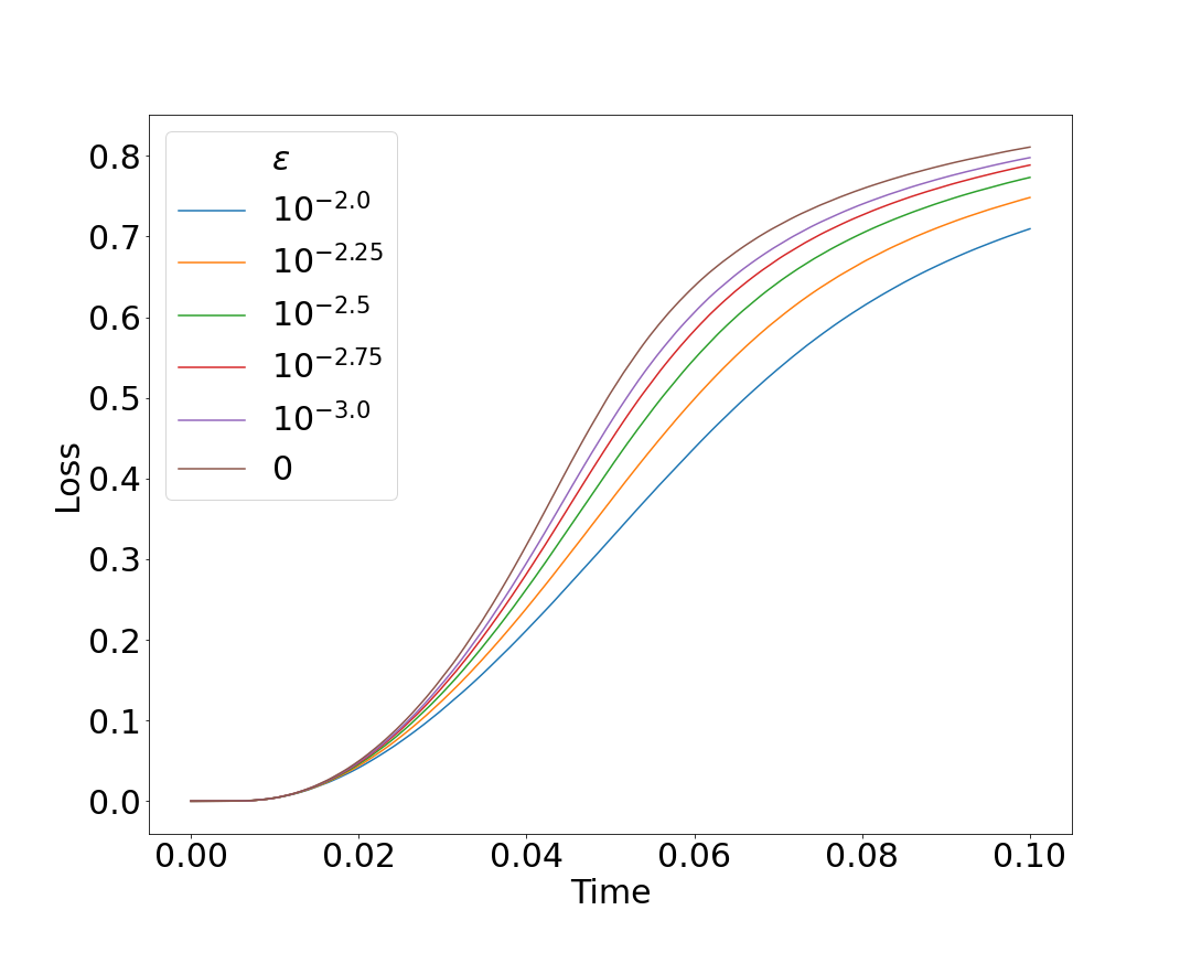
(a) $X_{0-}\sim^{d}\operatorname{Uniform}[0.25,\,0.35],\,\alpha=0.5$

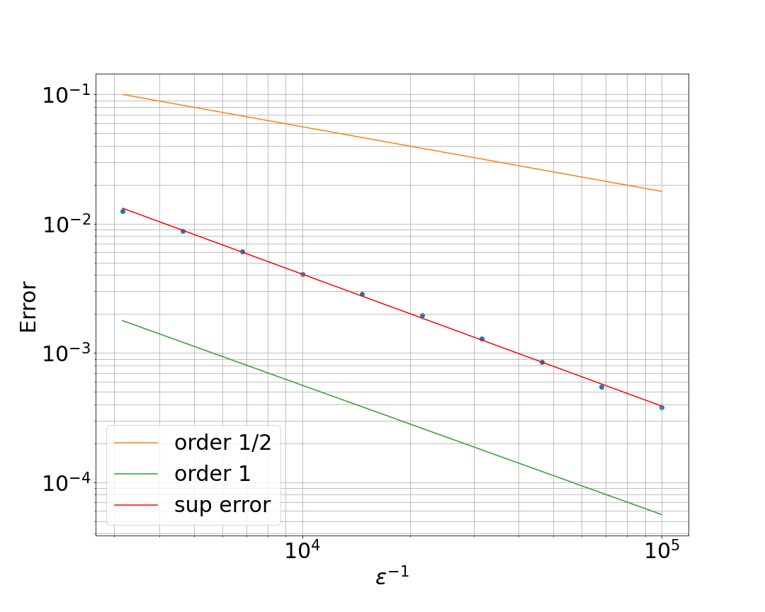
(b) Rate of Convergence

Figure 1: Initial density vanishing at zero with no discontinuity and common noise

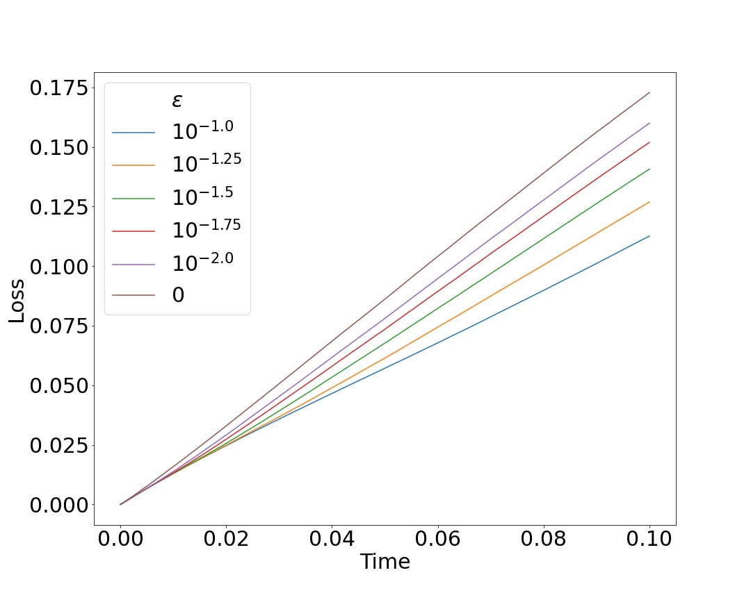
(c) $X_{0-}\sim^{d}\Gamma(2.1,\frac{1}{2}),\,\alpha=1.3$

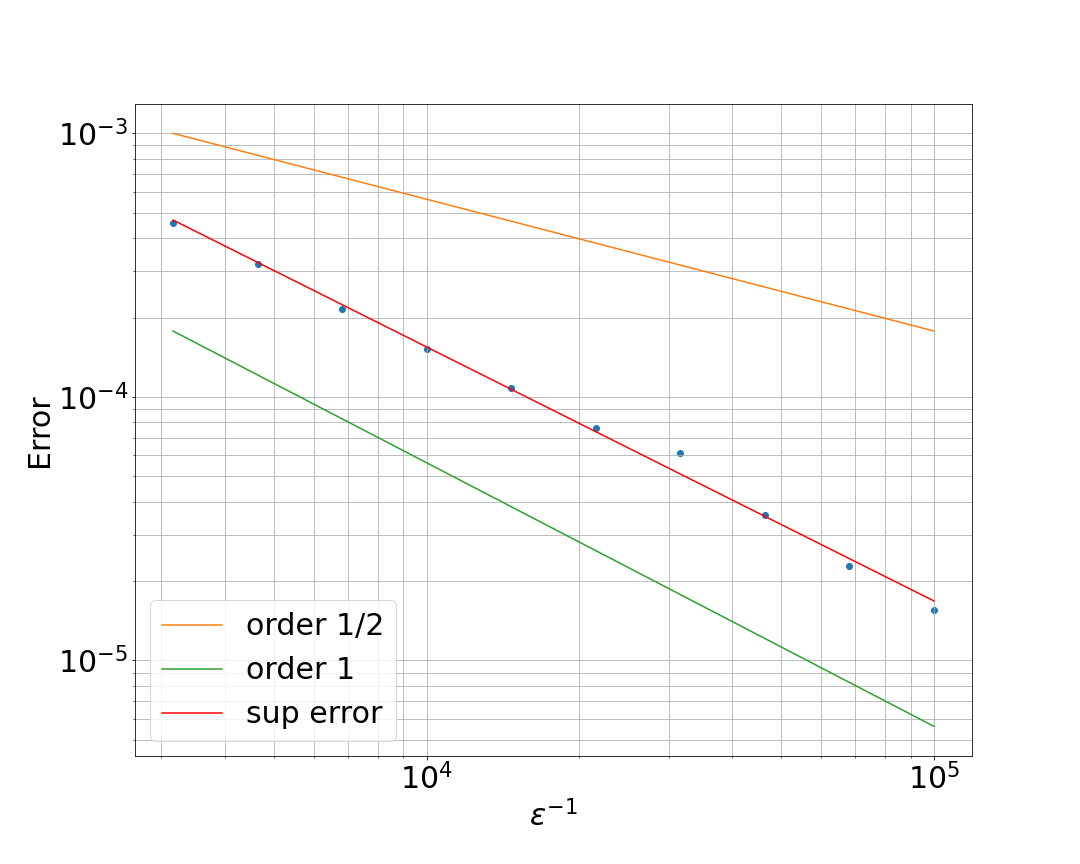
(d) Rate of Convergence

4.4 Setting with discontinuity and without common noise

To simulate a setting where we would see a systemic event, we changed the parameters of the Gamma distribution such that most of the mass will be near the boundary and made $\alpha$ sufficiently large. In Fig. 2(c), we conducted simulations using two different initial conditions. In the first case, we set $X_{0-}$ to follow a Gamma distribution with parameters $(1.2,0.5)$ and assigned $\alpha$ a value of 0.9. In the second case, $X_{0-}$ was generated from a Gamma distribution with parameters $(1.4,0.5)$, and $\alpha$ was set to 2. Within this particular setup, we observe a convergence rate between $1/2$ and $1$ prior to the occurrence of the first jump. The rate appears to be unaffected by the characteristics of the density of $X_{0-}$ near the boundary, despite the theoretical estimates relying on such information. Moreover, the theoretical estimates consistently predicted a convergence rate strictly below $1/2$ in all scenarios involving an initial condition of this form, in contrast to our empirical results, which indicate a convergence rate greater than $1/2$.

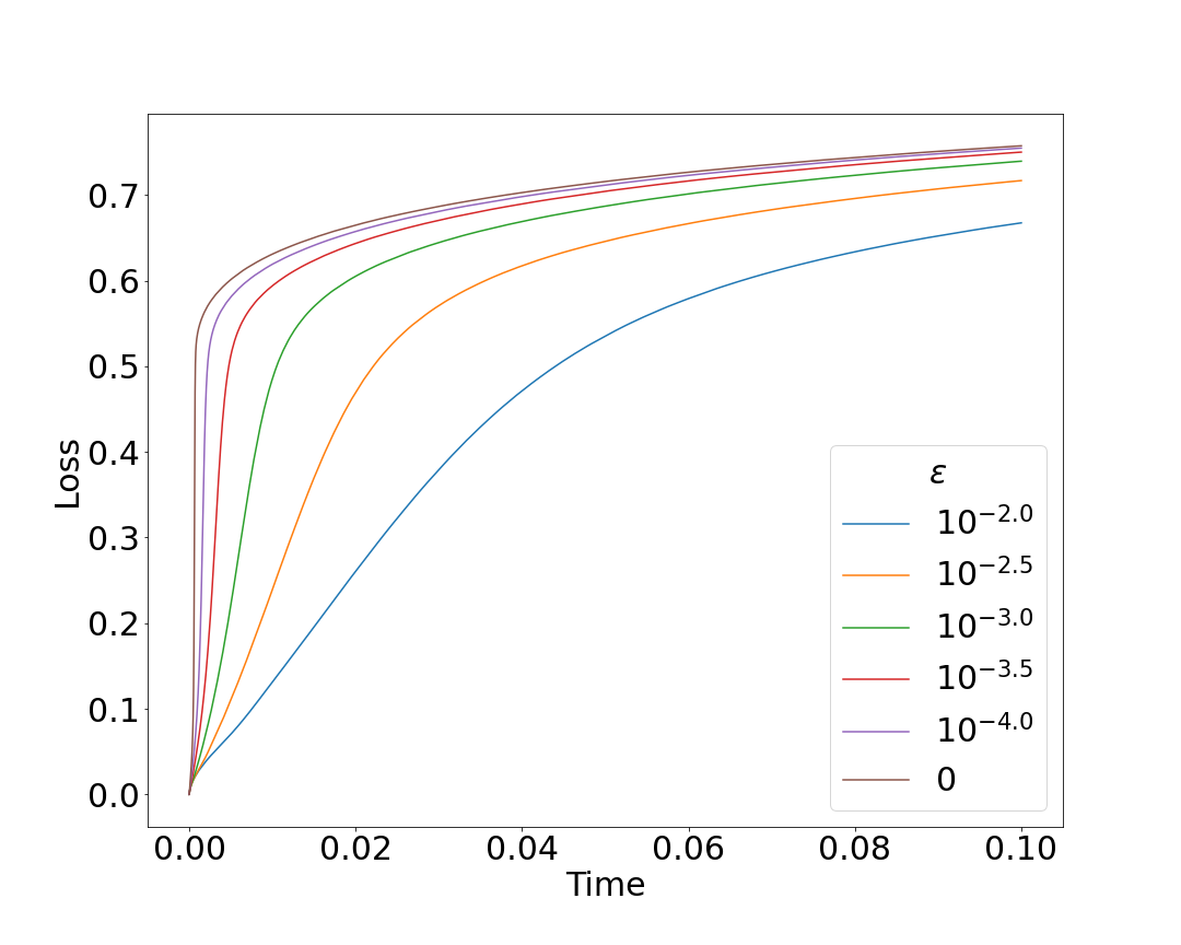
(a) $X_{0-}\sim^{d}\Gamma(1.2,0.5),\,\alpha=0.9$

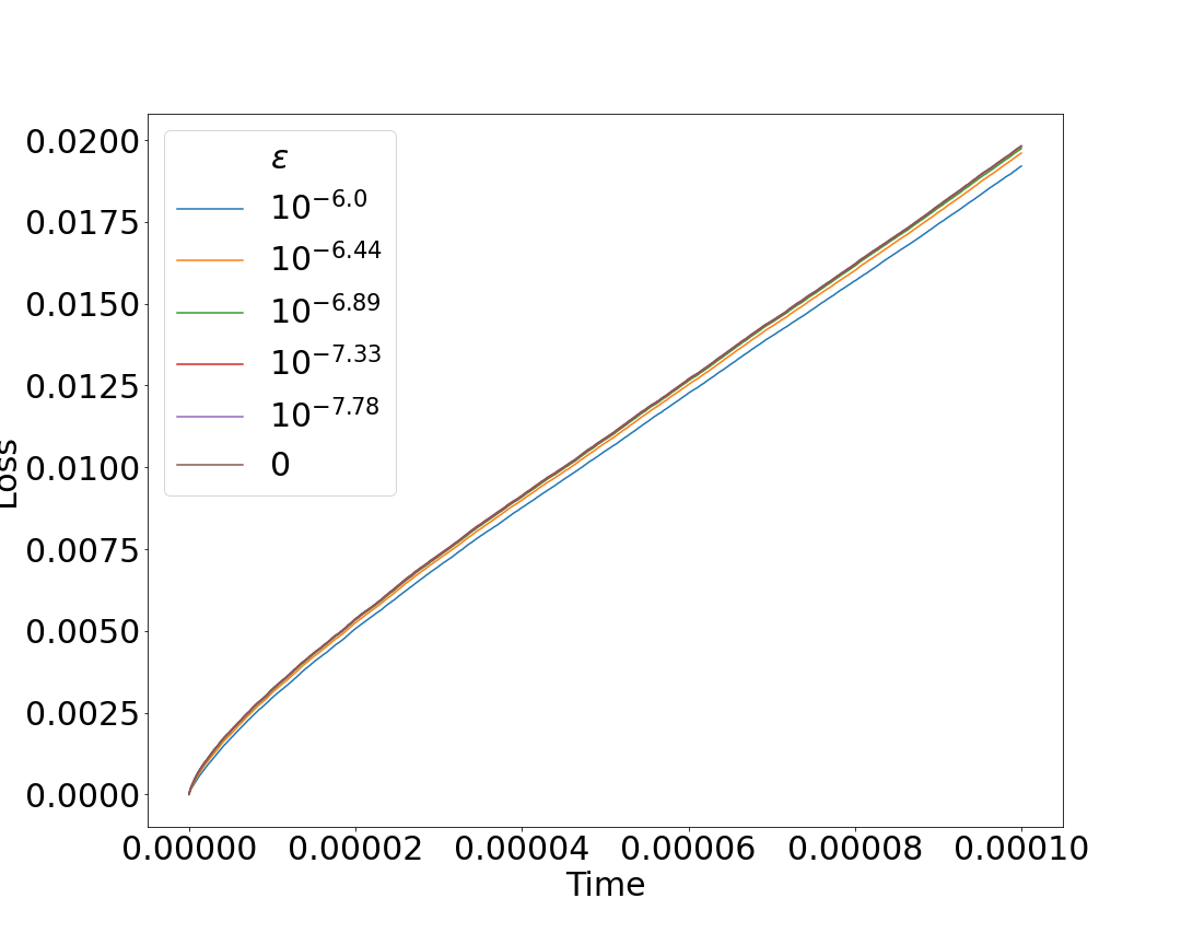
(b) $t_{max}=0.0001$

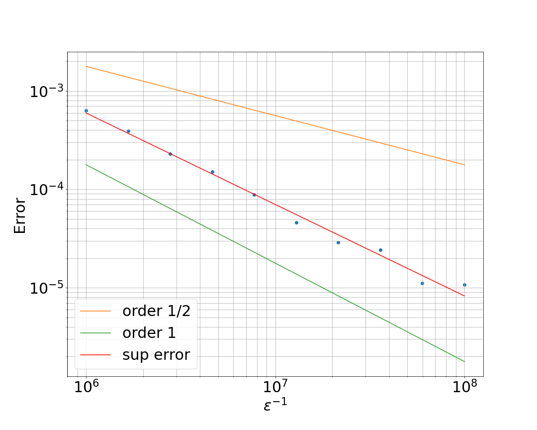
(c) Rate of Convergence

Figure 2: Initial density vanishing at zero with discontinuity and no common noise

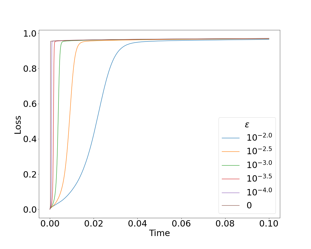
(d) $X_{0-}\sim^{d}\Gamma(1.4,0.5),\,\alpha=2$

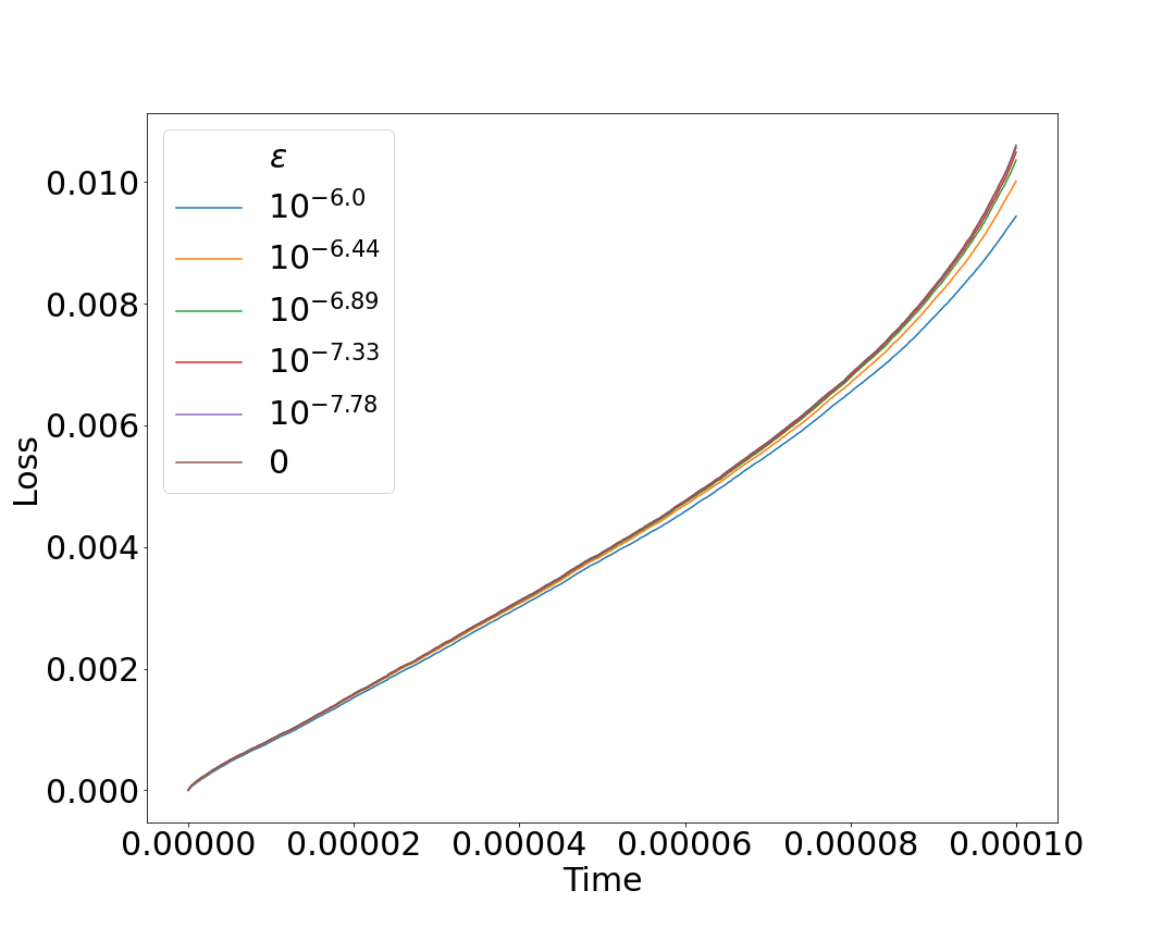
(e) $t_{max}=0.0001$

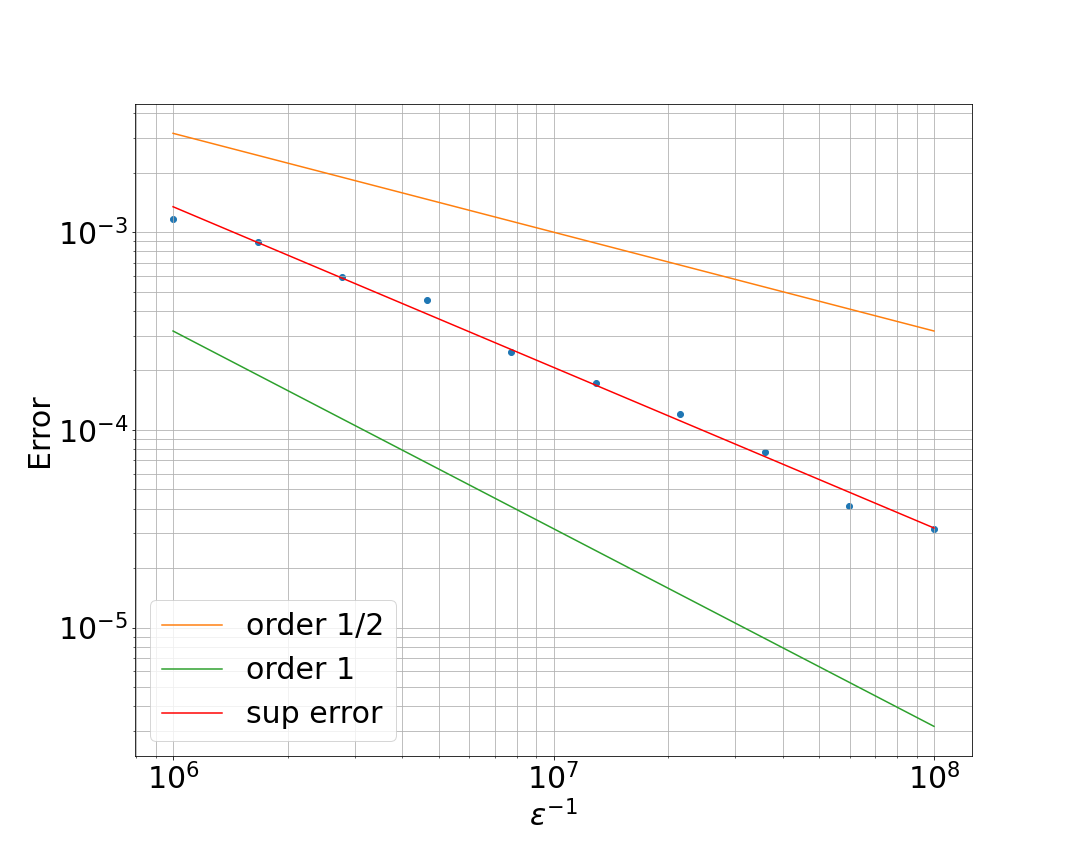
(f) Rate of Convergence

4.5 Simulations with common noise

Similar to the previous subsections, we conducted two experiments. In both experiments, we assigned $X_{0-}$ a uniform distribution over the interval $[0.25,0.35]$, set $\alpha$ to $0.5$ and $\rho$ to $0.5$. This initial condition is the same as in Section 4.3. However, we used different common noise paths for each experiment. In the first simulation, the common noise path increases to $1$ over the time domain. This led to the loss process becoming rougher than the loss in the previous setting. In the second simulation, the common noise path decreases to $-1$. This induces a systemic event due to the rapid loss of mass. Despite the differences between the scenarios, we observed a similar rate of convergence between $1/2$ and $1$ as illustrated in Fig. 3(c).

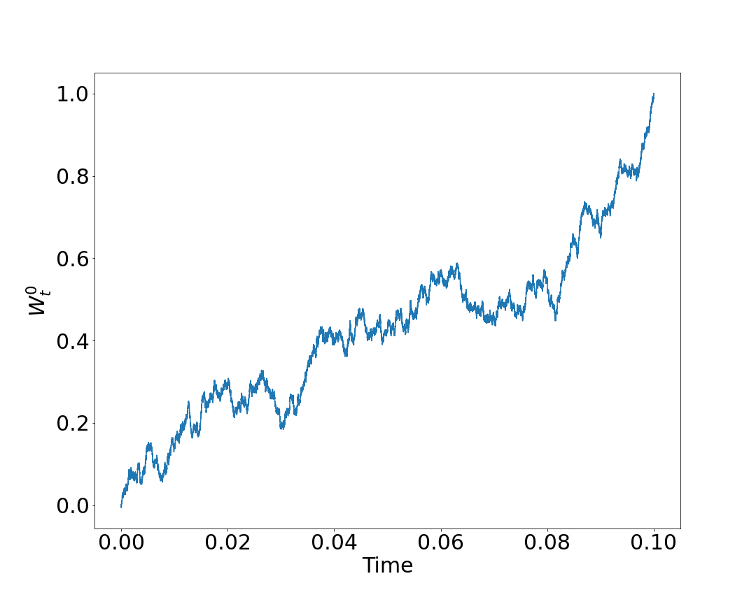
(a) Common Noise Path

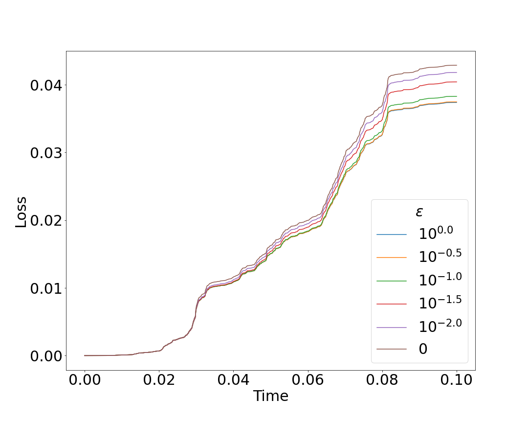
(b) $X_{0-}\sim^{d}\operatorname{Uniform}[0.25,\,0.35],\,\alpha=0.5$

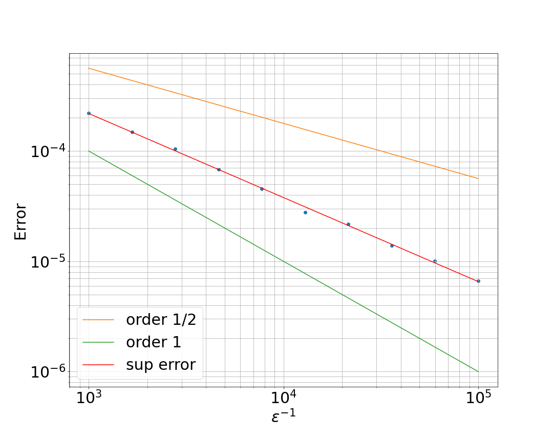
(c) Rate of Convergence

Figure 3: Initial density vanishing at zero with common noise

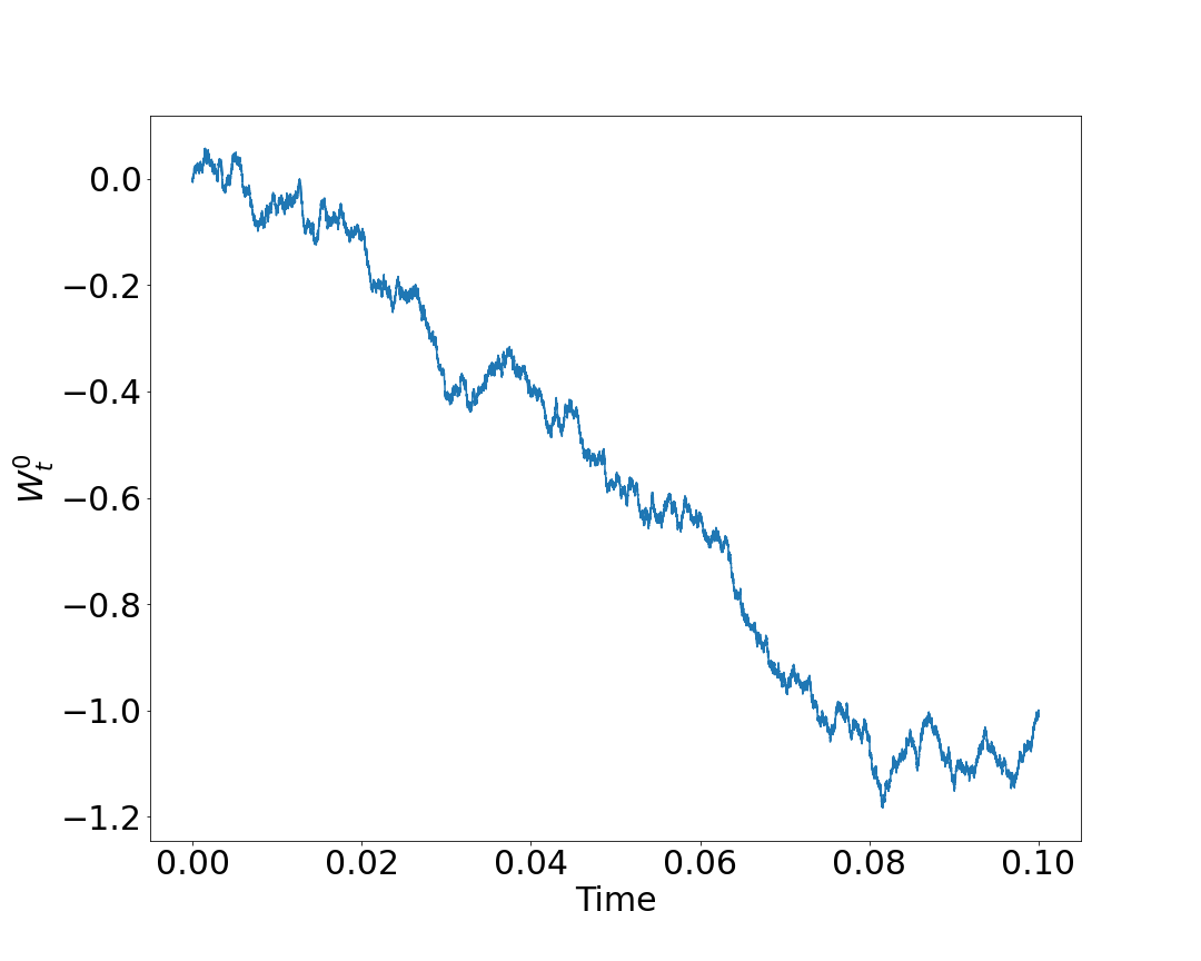
(d) Common Noise Path

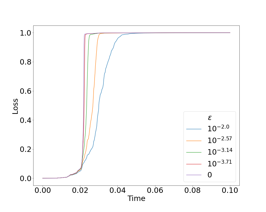
(e) $X_{0-}\sim^{d}\operatorname{Uniform}[0.25,\,0.35],\,\alpha=0.5$

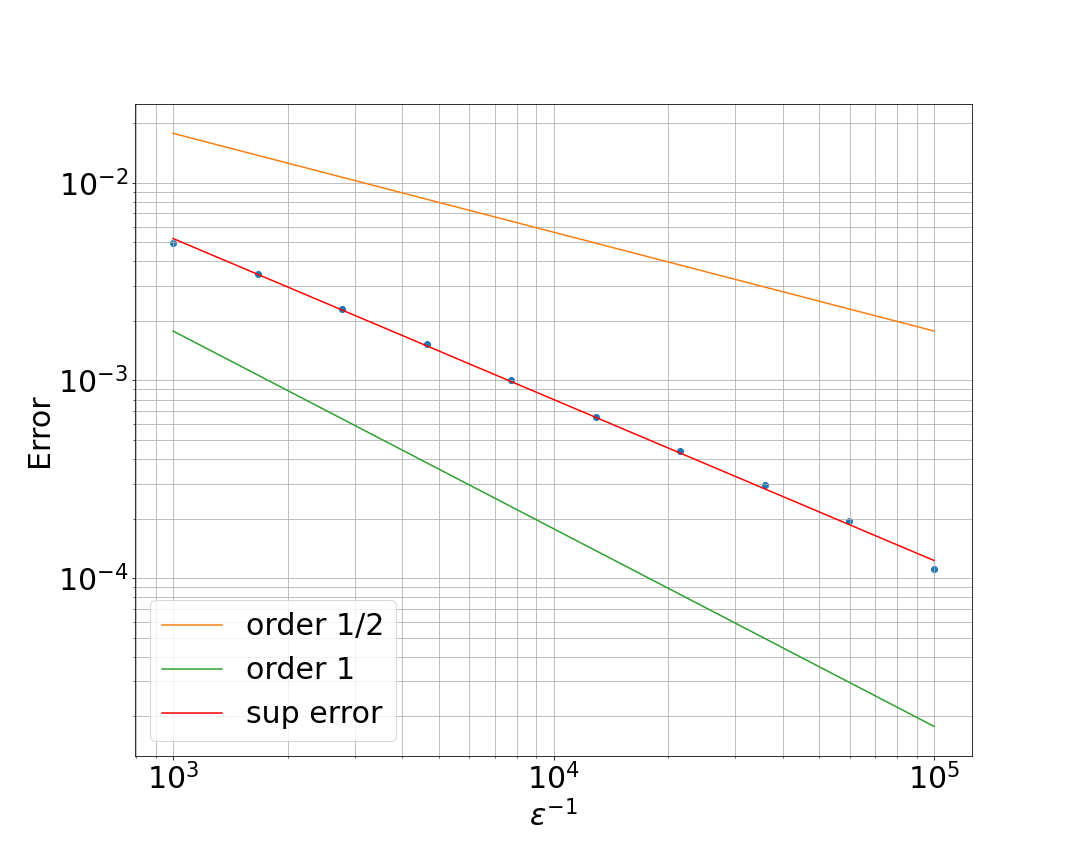
(f) Rate of Convergence

Appendix A Technical lemmas

Lemma A.1.

Suppose that $\tilde{P}^{\varepsilon_{n}}=\operatorname{Law}(\tilde{X}^{\varepsilon_{n}},\,\tilde{\mathcal{Y}}^{\varepsilon_{n}})$ converges weakly in $\mathcal{P}(D_{\mathbb{R}}\times\mathcal{C}_{\mathbb{R}})$ where $\tilde{X}^{\varepsilon_{n}},$ and $\tilde{\mathcal{Y}}^{\varepsilon_{n}}$ is the extension of ${X}^{\varepsilon_{n}}$ and ${\mathcal{Y}}^{\varepsilon_{n}}$. Let $X^{*}$ and $Y^{*}$ be the canonical processes on $D_{\mathbb{R}}\times\mathcal{C}_{\mathbb{R}}$ such that for $(\eta,\,\omega)\in D_{\mathbb{R}}\times\mathcal{C}_{\mathbb{R}}$, $X^{*}(\eta,\,\omega)=\eta$ and $Y^{*}(\eta,\,\omega)=\omega$. Then $Y^{*}$ is a martingale with respect to the filtration generated by $(X^{*},\,Y^{*})$ with quadratic variation

$$\left\langle Y^{*}\right\rangle_{t}=\begin{cases}\begin{aligned} &0&\qquad&t\in[-1,\,0)\\ &\int_{0}^{t}\sigma(s,\,X^{*}_{s})^{2}\mathop{}\!\mathrm{d}s&\qquad&t\in[0,\,T]\\ &\int_{0}^{t}\sigma(s,\,X_{s}^{*})^{2}\mathop{}\!\mathrm{d}s+(t-T)&\qquad&t\in(T,\,\bar{T}]\end{aligned}\end{cases}$$

Proof.

Set $\tilde{P}^{*}$ to be the limit point of $(\tilde{P}^{\varepsilon_{n}})_{n\geqslant 0}$ and

$$\mathbbm{T}^{\tilde{P}^{*}}\vcentcolon=\left\{t\in[-1,\,\bar{T}]\,;\,\tilde{P}^{*}(\eta_{t}=\eta_{t-})=1\right\}.$$

Now for any $s_{0},\,t_{0}\in\mathbbm{T}^{\tilde{P}^{*}}$ with $s_{0}<t_{0}$ and $\{s_{i}\}_{i=1}^{k}\subset[-1,\,s_{0}]\cap\mathbbm{T}^{\tilde{P}^{*}}$, we define the function

$$F\;:\;D_{\mathbb{R}}\times\mathcal{C}_{\mathbb{R}}\to\mathbb{R},\quad\eta,\omega\mapsto(\omega_{t_{0}}-\omega_{s_{0}})\prod_{i=1}^{k}f_{i}(\eta_{s_{i}},\omega_{s_{i}}),$$

for arbitrary $f_{i}\in\mathcal{C}_{b}(D_{\mathbb{R}}\times\mathcal{C}_{\mathbb{R}})$. In order to show that $Y^{*}$ is a martingale, it is sufficient to show that $\mathbb{E}^{\tilde{P}^{*}}[F(X^{*},\,Y^{*})]=0.$

As $\tilde{P}^{\varepsilon_{n}}\implies\tilde{P}^{*}$, then by Skohorod’s Representation Theorem, see [2, Theorem 7.6], there are $((x^{n},\,y^{n}))_{n\geqslant 1}$ and $(x,\,y)$ defined on the same background space such that $(x^{n},\,y^{n})$ converges to $(x,\,y)$ almost surely in $(D_{\mathbb{R}},\,\textnormal{M1})\times(\mathcal{C}_{\mathbb{R}},\,\left\lVert\cdot\right\rVert_{\infty})$ with $\operatorname{Law}(x^{n},\,y^{n})=\tilde{P}^{\varepsilon_{n}}$ and $\operatorname{Law}(x,y)=\tilde{P}^{*}$. Now for any $p>1$,

$$\mathbb{E}\left[\left|F(x^{n},\,y^{n})\right|\right]\leqslant C\mathbb{E}\left[\underset{s\leqslant\bar{T}}{\sup}|\tilde{\mathcal{Y}}_{s}^{\varepsilon_{n}}|\right]\leqslant C,$$

where $C$ is a constant that changes from line to line and depends only on $p,\,\sigma,\,T$ and the $f_{i}$’s but is independent of $\varepsilon$. Therefore $F(x^{n},\,y^{n})$ is uniformly $L^{p}$ bounded. For $t\in\{t_{0},\,s_{0},\,s_{1},\,\ldots,\,s_{k}\}$, it is an almost sure continuity point of $x$. Therefore by the properties of M1-convergence, $(x^{n}_{t},\,y^{n}_{t})$ converges to $(x_{t},\,y_{t})$ almost surely. Hence we have almost sure convergence of $F(x^{n},\,y^{n})$ to $F(x,\,y)$. Vitali’s Convergence Theorem states that almost sure convergence and uniform integrability implies convergence of means, hence

$$\mathbb{E}^{\tilde{P}^{*}}[F(X^{*},\,Y^{*})]=\mathbb{E}[F(x,\,y)]=\underset{n\xrightarrow[]{}\infty}{\lim}\mathbb{E}[F(x^{n},\,y^{n})]=\underset{n\xrightarrow[]{}\infty}{\lim}\mathbb{E}[F(\tilde{X}^{\varepsilon_{n}},\,\tilde{\mathcal{Y}}^{\varepsilon_{n}})]=0,$$

where the last inequality follows from the fact $\mathbb{E}[F(\tilde{X}^{\varepsilon_{n}},\,\tilde{\mathcal{Y}}^{\varepsilon_{n}})]=0$ for all $n$ as $\tilde{\mathcal{Y}}^{\varepsilon_{n}}$ is a martingale. Therefore by a monotone class theorem argument, $Y^{*}$ is a continuous local martingale.

Recall $x^{n}\xrightarrow[]{}x$ almost surely in $(D_{\mathbb{R}},\,\textnormal{M1})$, hence we have pointwise convergence at the continuity points of $x$, see [32, Theorem 12.5.1]. As $\sigma$ is in $\mathcal{C}^{1,\,2}$ by 2.2, there is a set of full probability such that $\sigma(s,x^{n}_{s})\xrightarrow[]{}\sigma(s,\,x_{s})$ for a set of $s$’s that have full Lebesgue measure in $[0,\,T]$. Furthermore, as $\sigma$ is bounded, by the Bounded Convergence Theorem

$$\int_{0}^{t}\sigma(s,\,x^{n}_{s})\mathop{}\!\mathrm{d}s\xrightarrow[]{}\int_{0}^{t}\sigma(s,\,x_{s})\mathop{}\!\mathrm{d}s$$ (A.1)

almost surely for any $t\in[0,\,T]$. Set

$$\left\langle Y\right\rangle_{t}=\begin{cases}\begin{aligned} &0&\qquad&t\in[-1,\,0)\\ &\int_{0}^{t}\sigma(s,\,X_{s})^{2}\mathop{}\!\mathrm{d}s&\qquad&t\in[0,\,T]\\ &\int_{0}^{t}\sigma(s,\,X_{s})^{2}\mathop{}\!\mathrm{d}s+(t-T)&\qquad&t\in(T,\,\bar{T}]\end{aligned}\end{cases}$$

where $Y$ is anyone of $Y^{*},\,y^{n}$ or $\tilde{\mathcal{Y}}^{\varepsilon_{n}}$ and $X$ is the respective $X^{*},\,x^{n}$ or $\tilde{X}^{\varepsilon_{n}}$. Employing Eq. A.1,

$$F(x^{n},\,(y^{n})^{2}-\langle y^{n}\rangle)\xrightarrow[]{}F(x,\,y^{2}-\langle y\rangle)\qquad\textnormal{almost surely.}$$

Also by above and the boundness of $\sigma$ by 2.2, $F(x^{n},\,(y^{n})^{2}-\langle y^{n}\rangle)$ is uniformly $L^{p}$ bounded in $n$. Hence by Vitali’s Convergence Theorem,

$$\mathbb{E}^{\tilde{P}^{*}}\left[F(X^{*},\,(Y^{*})^{2}-\langle Y^{*}\rangle)\right] =\mathbb{E}\left[F(x,\,y^{2}-\langle y\rangle)\right]$$

$$=\underset{n\xrightarrow[]{}\infty}{\lim}\mathbb{E}\left[F(x^{n},\,(y^{n})^{2}-\langle y^{n}\rangle)\right]$$

$$=\underset{n\xrightarrow[]{}\infty}{\lim}\mathbb{E}\left[F(\tilde{X}^{\varepsilon_{n}},\,(\tilde{\mathcal{Y}}^{\varepsilon_{n}})^{2}-\langle\tilde{\mathcal{Y}}^{\varepsilon_{n}}\rangle)\right]=0$$

where the last inequality follows from the fact that $(\tilde{\mathcal{Y}}^{\varepsilon_{n}})^{2}-\langle\tilde{\mathcal{Y}}^{\varepsilon_{n}}\rangle$ is true martingale from the boundness of $\sigma$. This completes the proof. ∎

Lemma A.2.

Consider the process $Z_{t}=M_{t}+tX$ for $t\in[-1,\,\bar{T}]$ where $M_{t}$ is a continuous local martingale with $c_{M}(t-s)\leqslant\langle M\rangle_{t}-\langle M\rangle_{s}\leqslant C_{m}(t-s)$ for any $0\leqslant s<t$ almost surely and $X$ is a non-negative random variable such that $\mathbb{E}[X]<\infty$. Then for any stopping time $\tau$ where $\tau\geqslant 0$ almost surely, then

$$\mathbb{P}\left[\underset{s\in(\tau,(\tau+h)\wedge\bar{T})}{\inf}\{Z_{s}-Z_{\tau}\}\geqslant 0,\,\tau<\bar{T}\right]=0,$$

for and $h>0$.

Proof.

In the case when $M$ is simply a Brownian motion, the result readily follows by the Stong Markov Property and standard properties of Brownian motion. As $M$ is a continuous local martingale, we may view it as a (random) time-changed Brownian motion. We exploit this fact to show the claim. To begin, fix a $\Delta\in(0,h)$, $\lambda>0$ and set $\bar{\tau}\vcentcolon=\tau\wedge(\bar{T}-\Delta)$. Then conditioning on the event $E\vcentcolon=\{\tau\leqslant\bar{T}-\Delta\}\cap\{X\leqslant\lambda\}$ and its complement

$$\begin{split}\mathbb{P}\left[\underset{s\in(\tau,(\tau+h)\wedge\bar{T})}{\inf}\{Z_{s}-Z_{\tau}\}>-\Delta,\,\tau<\bar{T}\right]&\leqslant\mathbb{P}\left[\underset{s\in(\bar{\tau},\bar{\tau}+\delta)}{\inf}\{M_{s}-M_{\bar{\tau}}+(s-\bar{\tau})\lambda\}>-\Delta\right]\\ &\qquad+\mathbb{P}\left[E^{\complement},\,\tau<\bar{T}\right]\end{split}$$ (A.2)

Focussing on the first term, we observe

$$\mathbb{P}\left[\underset{s\in(\bar{\tau},\bar{\tau}+\delta)}{\inf}\{M_{s}-M_{\bar{\tau}}+(s-\bar{\tau})\lambda\}>-\Delta\right]\leqslant\mathbb{P}\left[\underset{s\in(\bar{\tau},\bar{\tau}+\delta)}{\inf}\{M_{s}-M_{\bar{\tau}}\}>-\Delta(1+\lambda)\right]$$

By the Dubins-Schwarz Theorem, $M$ is a time-changed Brownian motion. Therefore there exists a Brownian Motion $B$ such that

$$\mathbb{P}\left[\underset{s\in(\bar{\tau},\bar{\tau}+\delta)}{\inf}\{M_{s}-M_{\bar{\tau}}\}>-\Delta(1+\lambda)\right]=\mathbb{P}\left[\underset{s\in(\bar{\tau},\bar{\tau}+\delta)}{\inf}\{B_{\langle M\rangle_{s}-\langle M\rangle_{\bar{\tau}}}\}>-\Delta(1+\lambda)\right]$$

Now as $\bar{\tau}=\tau\wedge(\bar{T}-\Delta)>0$ almost surely, $\langle M\rangle_{s}-\langle M\rangle_{\bar{\tau}}\geqslant c_{M}(s-\bar{\tau})$ for any $s>\bar{\tau}$ almost surely. So

$$\mathbb{P}\left[\underset{s\in(\bar{\tau},\bar{\tau}+\delta)}{\inf}\{B_{\langle M\rangle_{s}-\langle M\rangle_{\bar{\tau}}}\}>-\Delta(1+\lambda)\right]\leqslant\mathbb{P}\left[\underset{s\in(0,\Delta)}{\inf}\{B_{c_{M}s}\}>-\Delta(1+\lambda)\right]$$

By the reflection principle of Brownian motion, we have

$$\mathbb{P}\left[\inf_{s\leqslant\Delta}B_{c_{M}s}\leqslant-\Delta(1+\lambda)\right] =2\mathbb{P}\left[B_{\gamma c_{M}}\leqslant-\Delta(1+\lambda)\right]$$

$$=2(2\pi)^{-1/2}\int_{-\infty}^{-\Delta^{1/2}c_{M}^{-1/2}(1+\lambda)}e^{\frac{-y^{2}}{2}}\mathop{}\!\mathrm{d}y\geqslant 1-2\Delta^{1/2}(1+\lambda)(2\pi c_{M})^{-1/2}.$$

In conclusion, we have shown

$$\mathbb{P}\left[\underset{s\in(\bar{\tau},\bar{\tau}+\delta)}{\inf}\{M_{s}-M_{\bar{\tau}}+(s-\bar{\tau})\lambda\}>-\Delta\right]\leqslant\mathbb{P}\left[\underset{s\in(0,\Delta)}{\inf}\{B_{c_{M}s}\}>-\Delta(1+\lambda)\right]\leqslant 2\Delta^{1/2}(1+\lambda)(2\pi c_{M})^{-1/2}$$

Setting $\lambda=\Delta^{-1/4}$, then by continuity of measure and the above, the expression in (A.2) converges to 0 as we send $\Delta$ to zero. This completes the proof. ∎

Lemma A.3 (Convergence of Stopping Times).

Consider a sequence of functions $(z^{n})_{n\geqslant 1}$ in $D_{\mathbb{R}}$ converging towards some $z\in D_{\mathbb{R}}$ with respect to the $M1$-topology. We assume that $z$ has the following crossing property:

$$\forall\,h>0\;\tau_{0}(z)<\bar{T}\qquad\implies\qquad\inf_{s\in(\tau_{0}(z),(\tau_{0}(z)+h)\wedge\bar{T})}\left\{z_{s}-z_{\tau_{0}(z)}\right\}<0$$ (A.3)

where $\tau_{0}$ is defined as in Eq. 2.13 and $\Delta z_{t}\leqslant 0$ for all $t\in[-1,\bar{T}]$. Then we have

$$\lim_{n\to\infty}\tau_{0}(z^{n})=\tau_{0}(z)$$

Proof.

The proof is composed of two steps. We shall show that $\limsup_{n\to\infty}\tau_{0}(z^{n})\leqslant\tau_{0}(z)\leqslant\liminf_{n\to\infty}\tau_{0}(z^{n})$. Hence we will have equality and the claim follows.

Step 1: $\limsup_{n\to\infty}\tau_{0}(z^{n})\leqslant\tau_{0}(z)$
We define the set of continuity points of $z$ to be $\mathbbm{T}^{z}\vcentcolon=\{t\in[-1,\bar{T}];z_{t}=z_{t-}\}$. We remark that $\mathbbm{T}^{z}$ is co-countable by [2, Section 13]. As $\tau_{0}(z)<T$, by (A.3) for any fixed $m\in\mathbb{N}$ there exists a $t\in(\tau_{0}(z),(\tau_{0}(z)+1/m)\wedge\bar{T})\cap\mathbbm{T}^{z}$ such that $z_{t}<0$. Now, as $t$ is a continuity point of $z$, by [32, Theorem 12.5.1], we have that $z^{n}_{t}\xrightarrow[]{}z_{t}$ in $\mathbb{R}$ as $n\xrightarrow[]{}\infty$. Therefore for large $n$, $z_{t}^{n}<0$ hence

$$\limsup_{n\xrightarrow[]{}\infty}z_{t}^{n}\leqslant t\leqslant\tau_{0}(z)+\frac{1}{m}.$$

As $m\in\mathbb{N}$ was arbitrary, the claim follows.

Step 2: $\liminf_{n\to\infty}\tau_{0}(z^{n})\geqslant\tau_{0}(z)$
As $z^{n}\xrightarrow[]{}z$ in the $M1$-topology, we may find a sequence of parametric representations $((u^{n},r^{n}))_{n\geqslant 1}$ of $(z^{n})_{n\geqslant 1}$ which converges uniformly to a parametric representation $(u,r)$ of $z$, see [32, Theorem 12.5.1]. Therefore, we may find a $s^{n}\in[0,1]$ such that $(u^{n}_{s^{n}},r^{n}_{s^{n}})=(z^{n}_{\tau_{0}(z^{n})},\tau_{0}(z^{n}))$. By step 1, since $\tau_{0}(z)<\bar{T}$, we have have

$$\liminf_{n\xrightarrow[]{}\infty}\tau_{0}(z^{n})\leqslant\liminf_{n\xrightarrow[]{}\infty}\tau_{0}(z^{n})\leqslant\tau_{0}(z)<T.$$

Therefore by the finiteness of $\liminf_{n\xrightarrow[]{}\infty}\tau_{0}(z^{n})$ and compactness of $[0,1]$, we may find a subsequence $n_{k}$ such that $\tau_{0}(z^{n_{k}})\xrightarrow[]{}\liminf_{n\xrightarrow[]{}\infty}\tau_{0}(z^{n})$ and $s_{n_{k}}\xrightarrow[]{}s$ for some $s\in[0,1]$. By the uniform convergence of the parametric representations

$$\liminf_{k\xrightarrow[]{}\infty}z^{n_{k}}_{\tau_{0}(z^{n_{k}})} =\liminf_{k\xrightarrow[]{}\infty}u^{n_{k}}_{s^{n_{k}}}=u_{s},$$

$$\liminf_{k\xrightarrow[]{}\infty}\tau_{0}(z^{n_{k}}) =\liminf_{k\xrightarrow[]{}\infty}r^{n_{k}}_{s^{n_{k}}}=r_{s}.$$

As $r_{s}=\liminf_{n\xrightarrow[]{}\infty}\tau_{0}(z^{n})$, we may find $\gamma\in[0,1]$ such that $u_{s}=\gamma z_{(\liminf_{n\xrightarrow[]{}\infty}\tau_{0}(z^{n}))-}+(1-\gamma)z_{\liminf_{n\xrightarrow[]{}\infty}\tau_{0}(z^{n})}$. We also note $u_{s}\leqslant 0$ as $\liminf_{k\xrightarrow[]{}\infty}z^{n_{k}}_{\tau_{0}(z^{n_{k}})}\leqslant 0$. Lastly as $\Delta z_{t}\leqslant 0$ for all $t$, we have $z_{\liminf_{n\xrightarrow[]{}\infty}\tau_{0}(z^{n})}\leqslant 0$. Therefore, $\tau_{0}(z)\leqslant{\liminf_{n\xrightarrow[]{}\infty}\tau_{0}(z^{n})}$. This completes the proof. ∎

Lemma A.4 (Functional Continuity II).

Let $\mu\in\mathcal{P}(D_{\mathbb{R}})$ be any measure such that

$$\mu\left(\underset{s\in(\tau_{0}(\eta),\,(\tau_{0}(\eta)+h)\wedge\bar{T})}{\inf}\{\eta_{s}-\eta_{\tau_{0}(\eta)}\}\geqslant 0,\,\tau_{0}(\eta)<T\right)=0,$$ (A.4)

for any $h>0$. Then for any sequence of measures $(\mu^{n})_{n\geqslant 1}$ such that $\mu^{n}\implies\mu$ in $(\mathcal{P}(D_{\mathbb{R}}),\mathfrak{T}_{\text{M1}}^{\text{wk}})$, we have

$$\nu^{\mu^{n}}_{t}\vcentcolon=\mu^{n}(\eta_{t}\in\cdot,\,\tau_{0}(\eta)>t)\implies\nu^{\mu}_{t}\vcentcolon=\mu(\eta_{t}\in\cdot,\,\tau_{0}(\eta)>t),$$

in $\mathbf{M}_{\leqslant 1}(\mathbb{R})$, the space of sub-probability measures on $\mathbb{R}$ endowed with the topology of weak convergence, for and $t\geqslant 0$ such that $\mu(\eta_{t}=\eta_{t-})=1$ and $\mu(\tau_{0}(\eta)=t)=0$.

Proof.

The proof is an application of the Continuous Mapping Theorem, [2, Theorem 2.7]. We only need to construct $\mu$-almost sure continuous maps.

Step 1: Projection of measures from $D_{\mathbb{R}}$ to $\mathbb{R}\times\{0,\,1\}$
Consider the map

$$(X_{t},\,\mathbbm{1}_{\{\tau_{0}(\cdot)\}})\,:\,D_{\mathbb{R}}\to\mathbb{R}\times\{0,1\},\qquad\eta\mapsto(\eta_{t},\,\mathbbm{1}_{\{\tau_{0}(\eta)>t\}})$$ (A.5)

(A.5) is a $\mu$-almost sure continuous map. Choose a $\eta\in D_{\mathbb{R}}$ such that $\eta_{t}=\eta_{t-},\,\tau_{0}(\eta)\neq t$ and is in the complement of the event in (A.4). Such $\eta$’shave full measure under $\mu$. M1-convergence implies pointwise convergence at continuity points, [32, Theorem 12.5.1], therefore $X_{t}$ is M1-continuous for every such $\eta$. Also by Lemma 2.11, since (A.4) holds, $\tau_{0}$ is an M1-continuous map at $\eta$. As $\tau_{0}(\eta)\neq t$, $\mathbbm{1}_{\{\tau_{0}(\cdot)\}}$ is M1-continuous at $\eta$. Hence, $(X_{t},\,\mathbbm{1}_{\{\tau_{0}(\cdot)\}})$ is a $\mu$-almost sure continuous map. By the Continuous Mapping Theorem,

$$(X_{t},\,\mathbbm{1}_{\{\tau_{0}(\cdot)\}})^{\#}\mu^{n}\implies(X_{t},\,\mathbbm{1}_{\{\tau_{0}(\cdot)\}})^{\#}\mu\quad\text{in}\quad\mathcal{P}(D_{\mathbb{R}}\times\{0,\,1\}).$$

Step 2: Weak convergence of sub-probability measures
For any $f\in\mathcal{C}_{b}(\mathbb{R})$, define the map

$$\hat{f}\,:\,\mathbb{R}\times\{0,\,1\}\to\mathbb{R},\qquad(x,y)\mapsto f(x)\mathbbm{1}_{\{1\}}(y).$$

It is clear $\hat{f}\in\mathcal{C}_{b}(\mathbb{R}\times\{0,\,1\})$. By step 1,

$$\langle(X_{t},\,\mathbbm{1}_{\{\tau_{0}(\cdot)\}})^{\#}\mu^{n},\hat{f}\rangle\xrightarrow[]{}\langle(X_{t},\,\mathbbm{1}_{\{\tau_{0}(\cdot)\}})^{\#}\mu,\hat{f}\rangle.$$

But by definition, $\langle(X_{t},\,\mathbbm{1}_{\{\tau_{0}(\cdot)\}})^{\#}\mu^{n},\hat{f}\rangle=\nu^{\mu^{n}}_{t}(f)$ and $\langle(X_{t},\,\mathbbm{1}_{\{\tau_{0}(\cdot)\}})^{\#}\mu,\hat{f}\rangle=\nu^{\mu}_{t}(f)$. So $\nu^{\mu^{n}}_{t}(f)\xrightarrow[]{}\nu^{\mu}_{t}(f)$. The conclusion now follows by Portmanteau’s Theorem. ∎

Lemma A.5 (Weak convergence of sub-probability measures).

Suppose that $\tilde{\mathbf{P}}^{\varepsilon_{n}}\implies\tilde{\mathbf{P}}^{*}$ on $(\mathcal{P}(D_{\mathbb{R}}),\mathfrak{T}_{\text{M1}}^{\text{wk}})$ for a positive sequence $(\varepsilon_{n})_{n\geqslant 1}$ which converges to zero. Set

$$\mathbbm{T}\vcentcolon=\left\{t\in[-1,\bar{T}]\;:\;\mathbb{E}\left[\tilde{\mathbf{P}}^{*}(\eta_{t}=\eta_{t-})\right]=1,\,\mathbb{E}\left[\tilde{\mathbf{P}}^{*}(\tau_{0}(\eta)=t)\right]=0\right\}.$$

Then for any $t\in\mathbbm{T}$,

$$\bm{\nu}_{t}^{\varepsilon_{n}}\implies\bm{\nu}_{t}^{*}\vcentcolon=\tilde{\mathbf{P}}^{*}(\eta_{t}\in\cdot,\,\tau_{0}(\eta)>t)\quad\text{in}\quad\mathbf{M}_{\leqslant 1}(\mathbb{R}).$$

Proof.

By definition of $\mathbbm{T}$ and Lemma 2.9. for any $t\in\mathbbm{T}$ there is a set of $\mu$’s of full $\operatorname{Law}(\mathbf{P}^{*})$-measure such that

$$\mu(\eta_{t}=\eta_{t-}),\,\mu(\tau_{0}(\eta)=t)=0,\,\mu\left(\underset{s\in(\tau_{0}(\eta),\,(\tau_{0}(\eta)+h)\wedge T)}{\inf}\{\eta_{s}-\eta_{\tau_{0}(\eta)}\}\geqslant 0,\,\tau_{0}(\eta)<T\right)=0.$$ (A.6)

As $\tilde{\mathbf{P}}^{\varepsilon_{n}}\implies\tilde{\mathbf{P}}^{*}$, by Skohorod’s Representation Theorem there exists a $(\mathbf{Q}^{n})_{n\geqslant 1},\,\mathbf{Q}^{*}$ such that $\mathbf{Q}^{n}\xrightarrow[]{}\mathbf{Q}^{*}$ almost surely, $\operatorname{Law}(\mathbf{Q}^{n})=\operatorname{Law}(\tilde{\mathbf{P}}^{\varepsilon_{n}})$, $\operatorname{Law}(\mathbf{Q}^{*})=\operatorname{Law}(\tilde{\mathbf{P}}^{*})$ and $\mathbf{Q}^{*}$ satisfies (A.6) almost surely. Set

$$\nu_{t}^{\mathbf{Q}^{n}}=\mathbf{Q}^{n}(\eta_{t}\in\cdot,\,\tau_{0}(\eta)>t),\quad\text{and}\quad\nu_{t}^{\mathbf{Q}^{*}}=\mathbf{Q}^{*}(\eta_{t}\in\cdot,\,\tau_{0}(\eta)>t)$$

By Lemma A.4, $\nu_{t}^{\mathbf{Q}^{n}}\xrightarrow[]{}\nu_{t}^{\mathbf{Q}^{*}}$ almost surely in $\mathbf{M}_{\leqslant 1}(\mathbb{R})$. Now, for any $F\in\mathcal{C}_{b}(\mathbf{M}_{\leqslant 1}(\mathbb{R}))$, by the Dominated Convergence Theorem

$$\underset{n\xrightarrow[]{}\infty}{\lim}\mathbb{E}\left[F(\bm{\nu}_{t}^{\varepsilon_{n}})\right]=\underset{n\xrightarrow[]{}\infty}{\lim}\mathbb{E}\left[F(\nu_{t}^{\mathbf{Q}^{n}})\right]=\mathbb{E}\left[F(\nu_{t}^{\mathbf{Q}^{*}})\right]=\mathbb{E}\left[F(\bm{\nu}_{t}^{*})\right].$$

The result now follows by Portmanteau’s Theorem. ∎

Lemma A.6 (Functional Continuity III).

Let $\mu\in\mathcal{P}(D_{\mathbb{R}})$ be any measure such that

$$\mu\left(\underset{s\in(\tau_{0}(\eta),\,(\tau_{0}(\eta)+h)\wedge T)}{\inf}\{\eta_{s}-\eta_{\tau_{0}(\eta)}\}\geqslant 0,\,\tau_{0}(\eta)<\bar{T}\right)=0,$$ (A.7)

for any $h>0$ and let $g(t,x,\nu)$ be any function satisfying 2.2 i. Then $\int_{0}^{t}g(s,\eta_{s}^{n},\nu^{\mu^{n}}_{s})\mathop{}\!\mathrm{d}s$ converges to $\int_{0}^{t}g(s,\eta_{s},\nu^{\mu}_{s})\mathop{}\!\mathrm{d}s$ for any $t\geqslant 0$ whenever $(\eta^{n},\mu^{n})\xrightarrow[]{}(\eta,\mu)$ in $(\mathcal{P}(D_{\mathbb{R}}),\mathfrak{T}_{\text{M1}}^{\text{wk}})\times(D_{\mathbb{R}},\textnormal{M1})$ along a sequence for which $\sup_{n\geqslant 1}\langle\mu^{n},\,\sup_{s\leqslant\bar{T}}\left|\tilde{\eta}_{s}\right|^{p}\rangle<\infty$ for some $p>1$ and any $t\geqslant 0$. For any measure $m\in\mathcal{P}(D_{\mathbb{R}}),\,\nu_{s}^{m}\vcentcolon=m(\tilde{\eta}_{s}\in\cdot,\,\tau_{0}(\tilde{\eta})>s)$.

Proof.

By 2.2,

$$\left|g(s,\eta_{s}^{n},\nu_{s}^{\mu^{n}})\right|\leqslant C(1+\sup_{n\geqslant 1}\,\sup_{s\leqslant T}\left|\eta_{s}^{n}\right|+\sup_{n\geqslant 1}\langle\mu^{n},\,\sup_{s\leqslant T}\left|\tilde{\eta}_{s}\right|\rangle)$$ (A.8)

The R.H.S of (A.8) is finite because $\eta^{n}\xrightarrow[]{}\eta$ in $(D_{\mathbb{R}},\textnormal{M1})$ and by assumption. So it is sufficient to show $g(s,\eta_{s}^{n},\nu_{s}^{\mu^{n}})$ converges to $g(s,\eta_{s},\nu_{s}^{\mu})$ on a set of full Lebesgue measure. The conclusion then follows by the Dominated Convergence Theorem.

Choose an $s\in\mathbbm{T}^{\mu}\vcentcolon=\left\{t\in[-1,\bar{T}]\;:\;\mu(\eta_{t}=\eta_{t-})=1,\,\mu(\tau_{0}(\eta)=t)=0\right\}$. The by Lemma A.4, $\nu_{s}^{\mu^{n}}\implies\nu_{s}^{\mu}$. By Skohorod’s Representation Theorem, there exists a $(X^{n})_{n\geqslant 1},\,X$ defined on a common probability space such that $\operatorname{Law}(X^{n})-\nu_{s}^{\mu^{n}},\,\operatorname{Law}(X)-\nu_{s}^{\mu}$ and $X^{n}\xrightarrow[]{}X$ almost surely in $\mathbb{R}$. For any $\psi\in\mathcal{C}(\mathbb{R})$ with $\left\lVert\psi\right\rVert_{\operatorname{Lip}}\leqslant 1$ and $\left|\psi(0)\right|\leqslant 1$,

$$\left|\langle\right|\nu_{s}^{\mu^{n}}-\nu^{\mu},\,\psi\rangle=\left|\mathbb{E}\left[\psi(X^{n})-\psi(X)\right]\right|\leqslant\mathbb{E}\left|X^{n}-X\right|.$$

By assumption,

$$\mathbb{E}\left[\left|X^{n}\right|^{p}\right]=\langle\nu_{s}^{\mu^{n}},\,\left|\cdot\right|^{p}\rangle\leqslant\langle\mu^{n},\,\sup_{s\leqslant T}\left|\tilde{\eta}_{s}\right|^{p}\rangle<\infty,$$

uniformly in $n$ for some $p>1$. So $\left|X^{n}-X\right|$ is uniformly $L^{p}$-bounded and converges to zero almost surely. Therefore, by Vitali’s Convergence Theorem,

$$\underset{n\xrightarrow[]{}\infty}{\lim}d_{0}(\nu_{s}^{\mu^{n}},\,\nu_{s}^{\mu})=0$$ (A.9)

Lastly by 2.2,

$$\left|g(s,\eta_{s}^{n},\nu_{s}^{\mu^{n}})-g(s,\eta_{s},\nu_{s}^{\mu})\right|\leqslant C\left|\eta_{s}^{n}-\eta_{s}\right|+C(1+\left|\eta_{s}\right|+\langle\nu_{s}^{\mu^{n}},\,\left|\cdot\right|\rangle)d_{0}(\nu_{s}^{\mu^{n}},\,\nu_{s}^{\mu}).$$

As $s\in\mathbbm{T}^{\mu}$, the first term converges to zero as $\eta^{n}\xrightarrow[]{}\eta$ in $(D_{\mathbb{R}},\textnormal{M1})$. By assumption and (A.9), the second term converges to zero as $n\xrightarrow[]{}\infty$. This completes the proof. ∎

Lemma A.7.

Fix any $t<T$. There is a constant $C>0$ independent of $\varepsilon$ and $t$ such that for any $\gamma<1\wedge(T-t)$ we have

$$\mathbb{P}\left[\bm{\nu}_{t}^{\varepsilon}[0,\alpha_{t}z+C\gamma^{1/3}+\alpha_{t}(L_{t}^{\varepsilon}-\mathfrak{L}_{t}^{\varepsilon})+(\alpha_{t+\gamma}-\alpha_{t})]\geqslant z,\;\forall\;z\leqslant L_{t+\gamma}^{\varepsilon}-L_{t}^{\varepsilon}-C\gamma^{1/3}\right]\geqslant 1-C\gamma^{1/3}$$

Proof.

To begin, fix a $\gamma>0$ such that $\gamma<1\wedge(T-t)$ and fix a $z\in\mathbb{R}$. Then we define the event

$$E_{1}^{z}\vcentcolon=\Big{\{}X_{t}^{\varepsilon}-\gamma C(1+\underset{u\leqslant t+\gamma}{\sup}\left|X_{u}^{\varepsilon}\right|+\mathbb{E}[\underset{u\leqslant t+\gamma}{\sup}\left.\left|X_{u}^{\varepsilon}\right|\right|W^{0}])-\underset{u\leqslant\gamma}{\sup}\left|\mathcal{Y}^{\varepsilon}_{t+u}-\mathcal{Y}^{\varepsilon}_{t}\right|-\alpha_{t}z-\alpha_{t}(L_{t}^{\varepsilon}-\mathfrak{L}_{t}^{\varepsilon})-(\alpha_{t+\gamma}-\alpha_{t})\leqslant 0,\,\tau^{\varepsilon}>t\Big{\}}$$

where $C$ is the constant from the linear growth condition on $b$. Now fix $x\leqslant L_{t+\gamma}^{\varepsilon}-L_{t}^{\varepsilon}$. By the continuity of the loss process, [17, Theorem 2.4], there exists a $s\leqslant\gamma$ such that $x=L_{t+s}^{\varepsilon}-L_{t}^{\varepsilon}$. Employing the integration by parts formula, we observe for any $u\in[t,t+s]$

$$\int_{t}^{u}\alpha_{v}\mathop{}\!\mathrm{d}\mathfrak{L}_{v}^{\varepsilon} =\alpha_{u}\mathfrak{L}_{u}^{\varepsilon}-\alpha_{t}\mathfrak{L}_{t}^{\varepsilon}-\int_{t}^{u}\alpha^{\prime}(v)\mathfrak{L}_{v}^{\varepsilon}\mathop{}\!\mathrm{d}v\leqslant\alpha_{u}\mathfrak{L}_{u}^{\varepsilon}-\alpha_{t}\mathfrak{L}_{t}^{\varepsilon}$$

$$\leqslant\alpha_{t+s}{L}_{t+s}^{\varepsilon}-\alpha_{t}\mathfrak{L}_{t}^{\varepsilon}\leqslant\alpha_{t}{L}_{t+s}^{\varepsilon}+(\alpha_{t+s}-\alpha_{t})-\alpha_{t}\mathfrak{L}_{t}^{\varepsilon},$$

where to establish upper bounds we use the fact that $\alpha$ is non-negative and non-decreasing, and $\mathfrak{L}_{v}^{\varepsilon}\leqslant L_{v}^{\varepsilon}\leqslant 1$ for any $v\geqslant 0$. Therefore for any $u\in[t,t+s]$

$$X_{u}^{\varepsilon} =X_{t}^{\varepsilon}+(X_{u}^{\varepsilon}-X_{t}^{\varepsilon})=X_{t}^{\varepsilon}+\int_{t}^{u}b(v,X_{v}^{\varepsilon},\bm{\nu}_{v}^{\varepsilon})\mathop{}\!\mathrm{d}v+\mathcal{Y}_{u}-\mathcal{Y}_{t}-\int_{t}^{u}\alpha_{v}\mathop{}\!\mathrm{d}\mathfrak{L}_{v}^{\varepsilon}$$

$$\leqslant X_{t}^{\varepsilon}-\gamma C(1+\underset{u\leqslant t+\gamma}{\sup}\left|X_{u}^{\varepsilon}\right|+\mathbb{E}[\underset{u\leqslant t+\gamma}{\sup}\left.\left|X_{u}^{\varepsilon}\right|\right|W^{0}])-\underset{u\leqslant\gamma}{\sup}\left|\mathcal{Y}^{\varepsilon}_{t+u}-\mathcal{Y}^{\varepsilon}_{t}\right|$$

$$\qquad-\{\alpha_{t}{L}_{t+s}^{\varepsilon}+(\alpha_{t+s}-\alpha_{t})-\alpha_{t}\mathfrak{L}_{t}^{\varepsilon}\pm L_{t}^{\varepsilon}\}$$

$$\leqslant X_{t}^{\varepsilon}-\gamma C(1+\underset{u\leqslant t+\gamma}{\sup}\left|X_{u}^{\varepsilon}\right|+\mathbb{E}[\underset{u\leqslant t+\gamma}{\sup}\left.\left|X_{u}^{\varepsilon}\right|\right|W^{0}])-\underset{u\leqslant\gamma}{\sup}\left|\mathcal{Y}^{\varepsilon}_{t+u}-\mathcal{Y}^{\varepsilon}_{t}\right|$$

$$\qquad-\alpha_{t}x-(\alpha_{t+s}-\alpha_{t})-\alpha_{t}(L_{t}^{\varepsilon}-\mathfrak{L}_{t}^{\varepsilon})$$

Therefore as $L^{\varepsilon}$ is $W^{0}$ measurable and conditioning on $W^{0}$ fixes $L^{\varepsilon}$, we have

$$\mathbb{P}\left[\left.E_{1}^{x}\right|W^{0}\right]\geqslant\mathbb{P}\left[\left.\underset{t\leqslant u\leqslant t+s}{\inf}X_{u}^{\varepsilon}\leqslant 0,\tau^{\varepsilon}>t\right|W^{0}\right]=L_{t+s}^{\varepsilon}-L_{t}^{\varepsilon}=x.$$

Now, for any fixed $z\leqslant L_{t+\gamma}^{\varepsilon}-L_{t}^{\varepsilon}-2\gamma^{1/3}$, set $z_{0}=z+2\gamma^{1/3}$. We define the event

$$E_{2}\vcentcolon=\Big{\{}\gamma C(1+\underset{u\leqslant t+\gamma}{\sup}\left|X_{u}^{\varepsilon}\right|+\mathbb{E}[\underset{u\leqslant t+\gamma}{\sup}\left.\left|X_{u}^{\varepsilon}\right|\right|W^{0}])+\underset{u\leqslant\gamma}{\sup}\left|\mathcal{Y}^{\varepsilon}_{t+u}-\mathcal{Y}^{\varepsilon}_{t}\right|\geqslant\gamma^{1/3}\Big{\}}$$

Then on the event $E_{1}^{z_{0}}\cap E_{2}^{\complement}$

$$X_{t}^{\varepsilon}-\alpha_{t}z_{0} \leqslant\gamma C(1+\underset{u\leqslant t+\gamma}{\sup}\left|X_{u}^{\varepsilon}\right|+\mathbb{E}[\underset{u\leqslant t+\gamma}{\sup}\left.\left|X_{u}^{\varepsilon}\right|\right|W^{0}])+\underset{u\leqslant\gamma}{\sup}\left|\mathcal{Y}^{\varepsilon}_{t+u}-\mathcal{Y}^{\varepsilon}_{t}\right|+\alpha_{t}(L_{t}^{\varepsilon}-\mathfrak{L}_{t}^{\varepsilon})+(\alpha_{t+\gamma}-\alpha_{t})$$

$$\leqslant\gamma^{1/3}+\alpha_{t}(L_{t}^{\varepsilon}-\mathfrak{L}_{t}^{\varepsilon})+(\alpha_{t+\gamma}-\alpha_{t}).$$

Therefore on the same event

$$X_{t}^{\varepsilon}-\alpha_{t}z=X_{t}^{\varepsilon}-\alpha_{t}z_{0}+2\alpha_{t}\gamma^{1/3}\leqslant(1+2\alpha_{t})\gamma^{1/3}+\alpha_{t}(L_{t}^{\varepsilon}-\mathfrak{L}_{t}^{\varepsilon})+(\alpha_{t+\gamma}-\alpha_{t})$$

Consequently, we deduce

$$\bm{\nu}_{t}^{\varepsilon}[0,\alpha_{t}z+(1+2\alpha_{t})\gamma^{1/3}+\alpha_{t}(L_{t}^{\varepsilon}-\mathfrak{L}_{t}^{\varepsilon})+(\alpha_{t+\gamma}-\alpha_{t})] \geqslant\mathbb{P}\left[\left.E_{1}^{z_{0}}\cap E_{2}^{\complement}\right|W^{0}\right]$$

$$\geqslant\mathbb{P}\left[\left.E_{1}^{z_{0}}\right|W^{0}\right]-\mathbb{P}\left[\left.E_{2}\right|W^{0}\right]$$

$$\geqslant z_{0}-\mathbb{P}\left[\left.E_{2}\right|W^{0}\right].$$

Therefore if we have control over the mass $\mathbb{P}\left[\left.E_{2}\right|W^{0}\right]$, we may estimate the mass with respect to $\bm{\nu}_{t}$ that is near the boundary. Therefore, defining the event $E_{3}\vcentcolon=\{\mathbb{P}\left[\left.E_{2}\right|W^{0}\right]\leqslant\gamma^{1/3}\}$ we deduce on $E_{3}$

$$\bm{\nu}_{t}^{\varepsilon}[0,\alpha_{t}z+(1+2\alpha_{t})\gamma^{1/3}+\alpha_{t}(L_{t}^{\varepsilon}-\mathfrak{L}_{t}^{\varepsilon})+(\alpha_{t+\gamma}-\alpha_{t})]\geqslant z_{0}-\gamma^{1/3}\geqslant z.$$

The last inequality follows from the fact that $z_{0}=z+2\gamma^{1/3}$. Now we only need to find a $C$ independent of $\varepsilon,\,\gamma$ and $t$ such that $\mathbb{P}[E_{3}^{\complement}]\leqslant C\gamma^{1/3}$. By application of Markov’s inequality twice

$$\mathbb{P}\left[E_{3}^{\complement}\right] \leqslant\gamma^{-1/3}\mathbb{P}\left[E_{2}\right]$$

$$\leqslant\gamma^{-1/3}\mathbb{P}\left[\gamma C(1+\underset{u\leqslant t+\gamma}{\sup}\left|X_{u}^{\varepsilon}\right|+\mathbb{E}[\underset{u\leqslant t+\gamma}{\sup}\left.\left|X_{u}^{\varepsilon}\right|\right|W^{0}])\geqslant 2^{-1}\gamma^{1/3}/2\right]$$

$$\qquad+\gamma^{-1/3}\mathbb{P}\left[\underset{u\leqslant\gamma}{\sup}\left|\mathcal{Y}^{\varepsilon}_{t+u}-\mathcal{Y}^{\varepsilon}_{t}\right|\geqslant 2^{-1}\gamma^{1/3}/2\right]$$

$$\leqslant 2C\gamma^{1/3}\mathbb{E}\left[1+\underset{u\leqslant t+\gamma}{\sup}\left|X_{u}^{\varepsilon}\right|+\mathbb{E}[\underset{u\leqslant t+\gamma}{\sup}\left.\left|X_{u}^{\varepsilon}\right|\right|W^{0}]\right]+2^{8}\gamma^{-3}\mathbb{E}\left[\underset{u\leqslant\gamma}{\sup}\left|\mathcal{Y}^{\varepsilon}_{t+u}-\mathcal{Y}^{\varepsilon}_{t}\right|^{8}\right]$$

$$\leqslant c_{1}(\gamma^{1/3}+\gamma)\leqslant 2c_{1}\gamma^{1/3},$$

where $c_{1}$ depends on the constant from Proposition 2.6, the constant from Burkholder-Davis-Gundy to bound the second term and the uniform bounds on $\sigma$, but is notably independent of $\varepsilon$. Therefore, setting $C=\max\{1+2\alpha(T),c_{1}\}$ completes the proof. ∎

Lemma A.8.

Suppose that $\tilde{\mathbf{P}}^{\varepsilon_{n}}\implies\tilde{\mathbf{P}}^{*}$ on $(\mathcal{P}(D_{\mathbb{R}}),\mathfrak{T}_{\text{M1}}^{\text{wk}})$ for a positive sequence $(\varepsilon_{n})_{n\geqslant 1}$ which converges to zero. Set

$$\mathbbm{T}\vcentcolon=\left\{t\in[-1,\bar{T}]\;:\;\mathbb{E}\left[\tilde{\mathbf{P}}^{*}(\eta_{t}=\eta_{t-})\right]=1,\,\mathbb{E}\left[\tilde{\mathbf{P}}^{*}(\tau_{0}(\eta)=t)\right]=0\right\}.$$

Then for any $t\in\mathbbm{T}\cap[0,T)$ and $\gamma>0$ such that $t+\gamma\in\mathbbm{T}\cap[0,T)$ we have

$$\mathbb{P}\left[\bm{\nu}_{t}[0,\alpha(t)z+C\gamma^{1/3}+\alpha(t+\gamma)-\alpha(t)]\geqslant z,\;\forall\;z\leqslant L_{t+\gamma}-L_{t}-C\gamma^{1/3}\right]\geqslant 1-C\gamma^{1/3}$$

Proof.

As $\tilde{\mathbf{P}}^{\varepsilon_{n}}\implies\tilde{\mathbf{P}}^{*}$, by employing Skohorod’s Representation Theorem, there exists a $(\bm{\mu}^{n})_{n\geqslant 1}$ and $\bm{\mu}$ such that $\operatorname{Law}(\bm{\mu}^{n})=\operatorname{Law}(\tilde{\mathbf{P}}^{\varepsilon_{n}})$, $\operatorname{Law}(\bm{\mu})=\operatorname{Law}(\tilde{\mathbf{P}}^{*})$ and $\bm{\mu}^{n}\xrightarrow[]{}\bm{\mu}$ almost surely in $(\mathcal{P}(D_{\mathbb{R}}),\mathfrak{T}_{\textnormal{M1}}^{\text{wk}})$. As $\operatorname{Law}(\mathbf{P}^{*})$-almost every measure $\mu$ satisfy Eq. A.4 by Lemma 2.9, then by Lemma A.4 $\nu_{t}^{\bm{\mu}^{n}}\xrightarrow[]{}\nu_{t}^{\bm{\mu}}$ almost surely for any $t\in\mathbbm{T}$. Furthermore for any $t\in\mathbbm{T}\cap[0,T)$, by Lemma 2.11 and Corollary 2.12, we have

$$\bm{\mu}^{n}(\tau_{0}(\eta)\leqslant t)\xrightarrow[]{}\bm{\mu}(\tau_{0}(\eta)\leqslant t)\quad\textnormal{and}\quad\int_{0}^{t}\kappa^{\varepsilon_{n}}(t-s)\bm{\mu}^{n}(\tau_{0}(\eta)\leqslant s)\mathop{}\!\mathrm{d}s\xrightarrow[]{}\int_{0}^{t}\kappa^{\varepsilon_{n}}(t-s)\bm{\mu}(\tau_{0}(\eta)\leqslant s)\mathop{}\!\mathrm{d}s$$

almost surely. Therefore for simplicity and notational convenience for the remainder of this proof, we may suppose

$$\bm{\nu}_{t}^{\varepsilon_{n}}\xrightarrow[]{}\bm{\nu}_{t} \textnormal{a.s. in }\mathbf{M}_{\leqslant 1}(\mathbb{R}),$$

$$L_{t}^{\varepsilon_{n}}\xrightarrow[]{}L_{t} \textnormal{a.s. in }\mathbb{R},$$

$$\mathfrak{L}_{t}^{\varepsilon_{n}}\xrightarrow[]{}{L}_{t} \textnormal{a.s. in }\mathbb{R}.$$

Recall by Lemma A.7,

$$\mathbb{P}\left[\bm{\nu}_{t}^{\varepsilon}[0,\alpha_{t}z+C\gamma^{1/3}+\alpha_{t}(L_{t}^{\varepsilon}-\mathfrak{L}_{t}^{\varepsilon})+(\alpha_{t+\gamma}-\alpha_{t})]\geqslant z,\;\forall\;z\leqslant L_{t+\gamma}^{\varepsilon}-L_{t}^{\varepsilon}-C\gamma^{1/3}\right]\geqslant 1-C\gamma^{1/3},$$

for any $\varepsilon>0$. It is well known that the Levy-Prokhorov metric, $d_{L}$, metricizes weak convergence, [29, Theorem 1.11]. Fixing $\delta_{1},\,\delta_{2},\,\delta_{3},\,\delta_{4}>0$, we define the event

$$A_{n}\vcentcolon=\left\{\left|L_{t}^{\varepsilon_{n}}-L_{t}\right|<\delta_{1},\left|L_{t+\gamma}^{\varepsilon_{n}}-L_{t+\gamma}\right|<\delta_{2},\left|\mathfrak{L}_{t}^{\varepsilon_{n}}-L_{t}^{\varepsilon_{n}}\right|<\delta_{3},d_{L}(\bm{\nu}_{t}^{\varepsilon_{n}},\bm{\nu}_{t})<\delta_{4}\right\}$$

Therefore

$$1-C\gamma^{1/3} \leqslant\mathbb{P}\left[\bm{\nu}_{t}^{\varepsilon_{n}}[0,\alpha_{t}z+C\gamma^{1/3}+\alpha_{t}(L_{t}^{\varepsilon_{n}}-\mathfrak{L}_{t}^{\varepsilon_{n}})+(\alpha_{t+\gamma}-\alpha_{t})]\geqslant z,\;\forall\;z\leqslant L_{t+\gamma}^{\varepsilon_{n}}-L_{t}^{\varepsilon_{n}}-C\gamma^{1/3}\right]$$

$$\quad+\mathbb{P}[A_{n}^{\complement}]$$

$$\leqslant\mathbb{P}\left[\delta_{4}+\bm{\nu}_{t}(-\delta_{4},\alpha_{t}z+C\gamma^{1/3}+\alpha_{t}\gamma_{3}+(\alpha_{t+\gamma}-\alpha_{t})+\delta_{4})\geqslant z,\;\forall\;z\leqslant L_{t+\gamma}-L_{t}-C\gamma^{1/3}-\delta_{1}-\delta_{2}\right]$$

$$\quad+\mathbb{P}[A_{n}^{\complement}]$$

Sending $\varepsilon_{n}\xrightarrow[]{}0$, then $\mathbb{P}[A_{n}^{\complement}]\xrightarrow[]{}0$ by the Dominated Convergence Theorem as we have almost sure convergence. Lasts by sending $\delta_{1}\xrightarrow[]{}0,\,\delta_{2}\xrightarrow[]{}0,\,\delta_{3}\xrightarrow[]{}0,\,\delta_{4}\xrightarrow[]{}0$ one at a time and in order, then by employing continuity of measure we may conclude

$$\mathbb{P}\left[\bm{\nu}_{t}[0,\alpha_{t}z+C\gamma^{1/3}+(\alpha_{t+\gamma}-\alpha_{t})]\geqslant z,\;\forall\;z\leqslant L_{t+\gamma}-L_{t}-C\gamma^{1/3}\right]\geqslant 1-C\gamma^{1/3}$$

∎

Lemma A.9.

Suppose that $\tilde{\mathbf{P}}^{\varepsilon_{n}}\implies\tilde{\mathbf{P}}^{*}$ on $(\mathcal{P}(D_{\mathbb{R}}),\mathfrak{T}_{\text{M1}}^{\text{wk}})$ for a positive sequence $(\varepsilon_{n})_{n\geqslant 1}$ which converges to zero. Then we have

$$L_{t}\leqslant\inf\left\{x\geqslant 0\,;\,\bm{\nu}_{t-}[0,\,\alpha(t)x]<x\right\}$$ (A.10)

almost surely for any $t\in[0,\,T)$.

Proof.

It is clear that Lemma A.9 holds for any $t\in\mathbbm{T}$. Hence we must only show the upper bound for $t\not\in\mathbbm{T}$. We first consider the case when $t\in(0,T)\cap\mathbbm{T}^{\complement}$. The case when $t=0$ will be treated separately. Now as $\mathbbm{T}$ is dense in $[0,T]$, we may find a $(t_{n})_{n\geqslant 1},\,(t_{n}+\gamma_{n})_{n\geqslant 1}\subset\mathbbm{T}$ such that $t_{n}\uparrow t$, $t_{n}+\gamma_{n}\downarrow t$ and $\gamma_{n}<2^{-3n}$. Now by the Borel-Cantelli Lemma, we have a set of full measure such that

$$\bm{\nu}_{t_{n}}[0,\alpha_{t_{n}}z+C\gamma_{n}^{1/3}+(\alpha_{{t_{n}}+\gamma_{n}}-\alpha_{t_{n}})]\geqslant z,\;\forall\;z\leqslant L_{{t_{n}}+\gamma_{n}}-L_{t_{n}}-C\gamma_{n}^{1/3},$$ (A.11)

for all (possibly stochastic) $n$ large. Furthermore, by the dominated convergence theorem, we have

$$\bm{\nu}_{t_{n}}\xrightarrow[]{}\bm{\nu}_{t-},$$ (A.12)

$\operatorname{Law}(\tilde{\mathbf{P}}^{*})$-almost surely in $\mathbf{M}_{\leqslant 1}(\mathbb{R})$ as for any $\phi\in\mathcal{C}_{b}(\mathbb{R})$

$$\lim_{n\xrightarrow[]{}\infty}\bm{\nu}_{t_{n}}(\phi)=\lim_{n\xrightarrow[]{}\infty}\int_{D_{\mathbb{R}}}\phi(\eta_{t_{n}})\mathbbm{1}_{\{\tau_{0}(\eta)>t_{n}\}}\mathop{}\!\mathrm{d}\tilde{\mathbf{P}}^{*}(\eta)=\int_{D_{\mathbb{R}}}\phi(\eta_{t-})\mathbbm{1}_{\{\tau_{0}(\eta)\geqslant t\}}\mathop{}\!\mathrm{d}\tilde{\mathbf{P}}^{*}(\eta).$$

So on an event of full $\operatorname{Law}(\mathbf{P}^{*})$ measure where Eq. A.11 and Eq. A.12 holds, by Portmanteau Theorem for any $\gamma>0$, $z<\Delta L_{t}$

$$\bm{\nu}_{t-}[0,\,\alpha(t)z+\gamma]\geqslant\limsup_{n\xrightarrow[]{}\infty}\bm{\nu}_{t_{n}}[0,\,\alpha(t)z+\gamma]\geqslant\limsup_{n\xrightarrow[]{}\infty}\bm{\nu}_{t_{n}}[0,\alpha_{t_{n}}z+C\gamma_{n}^{1/3}+(\alpha_{{t_{n}}+\gamma_{n}}-\alpha_{t_{n}})]\geqslant z.$$

This holds as $z<\Delta L_{t}$ and $L_{{t_{n}}+\gamma_{n}}-L_{t_{n}}-C\gamma_{n}^{1/3}\xrightarrow[]{}\Delta L_{t}$. Sending $\gamma$ to zero shows the claim for every $t>0$.

In the case when $t=0$, we have by Lemma A.7

$$\mathbb{P}\left[\bm{\nu}_{0-}^{\varepsilon}[0,\alpha_{0}z+C\gamma^{1/3}+(\alpha_{\gamma}-\alpha_{0})]\geqslant z,\;\forall\;z\leqslant L_{\gamma}^{\varepsilon}-C\gamma^{1/3}\right]\geqslant 1-C\gamma^{1/3}.$$

As $\bm{\nu}^{\varepsilon}_{0-}=\nu_{0-}$, where $\nu_{0-}$ is a deterministic measure, and $\bm{nu}_{0-}$ is almost surely distributed as $\nu_{0-}$ almost surely, then we have by Lemma A.8

$$\mathbb{P}\left[\bm{\nu}_{0-}[0,\alpha(0)z+C\gamma^{1/3}+\alpha(\gamma)-\alpha(0)]\geqslant z,\;\forall\;z\leqslant L_{\gamma}-C\gamma^{1/3}\right]\geqslant 1-C\gamma^{1/3}.$$

for $\gamma\in\mathbbm{T}$. Now the rest of the proof follows similar arguments as above by choosing $\gamma_{n}\in\mathbbm{T}$ such that $\gamma_{n}\downarrow 0$. ∎

Proposition A.10 (Gronwall Type Inequality I).

Suppose $a,\,\tilde{\alpha},\,\tilde{\beta}\in\mathbb{R}_{+}$ such that $a\geqslant 0,\,0<\tilde{\beta}<1,\,\tilde{\alpha}>0$. Suppose $g(t)$ is a nonnegative, nondecreasing continuous function defined on $0\leqslant t<T$, $g(t)\leqslant M$ (constant), and suppose $u(t)$ is nonnegative and bounded on $0\leqslant t<T$ with

$$u(t)\leqslant a+g(t)\int_{0}^{t}(t-s)^{\tilde{\beta}-1}s^{\tilde{\alpha}-1}u(s)\mathop{}\!\mathrm{d}{}s$$

on this interval. Then

$$u(t)\leqslant a\left[1+\sum_{n\geqslant 1}g_{t}^{n}C_{n}t^{n(\tilde{\alpha}+\tilde{\beta}-1)}\right],\quad 0\leqslant t<T,$$

where

$$C_{0\phantom{+1}} \vcentcolon=1,$$

$$C_{1\phantom{+1}} \vcentcolon=B(\tilde{\alpha},\tilde{\beta}),$$

$$C_{n+1} \vcentcolon=B\left((n+1)\tilde{\alpha}+n\tilde{\beta}-n,\tilde{\beta}\right)C_{n},$$

$$B(\tilde{\alpha},\,\tilde{\beta}) \vcentcolon=\int_{0}^{1}(1-\tilde{s})^{\tilde{\beta}-1}\tilde{s}^{\tilde{\alpha}-1}\mathop{}\!\mathrm{d}{}\tilde{s}.$$

Proof.

Let $B\phi_{t}=g_{t}\int_{0}^{t}(t-s)^{\tilde{\beta}-1}s^{\tilde{\alpha}-1}\phi_{s}\mathop{}\!\mathrm{d}{}s$, $t\geqslant 0$, for localling integrable functions $\phi$. Then $u_{t}\leqslant a(t)+Bu_{t}$ implies

$$u_{t}\leqslant\sum_{k=0}^{n-1}B^{k}a+B^{n}u_{t}.$$

Let us prove that

$$B^{n}(1)_{t}\leqslant_{n}t^{n(\tilde{\alpha}+\tilde{\beta}-1)}g_{t}^{n}$$ (A.13)

and $B^{n}u_{t}\rightarrow 0$ as $n\rightarrow+\infty$ for each t in $0\leqslant t<T$.
Step 1: $B^{n}(1)_{t}\leqslant C_{n}t^{n(\tilde{\alpha}+\tilde{\beta}-1)}g_{t}^{n}$. For $n=1$,

$$B(1)_{t} =g_{t}\int_{0}^{t}(t-s)^{\tilde{\beta}-1}s^{\tilde{\alpha}-1}\mathop{}\!\mathrm{d}{}s,\quad\text{set }\tilde{s}=s/t$$

$$=g_{t}\int_{0}^{1}t^{\tilde{\beta}-1}(1-\tilde{s})^{\tilde{\beta}-1}t^{\tilde{\alpha}-1}\tilde{s}^{\tilde{\alpha}-1}t\mathop{}\!\mathrm{d}{}\tilde{s}$$

$$=g_{t}t^{\tilde{\alpha}+\tilde{\beta}-1}B(\tilde{\alpha},\,\tilde{\beta}).$$

Now, suppose the claim is true for $n=k$, then for $n=k+1$

$$B^{k+1}(1)_{t} =g_{t}\int_{0}^{t}(t-s)^{\tilde{\beta}-1}s^{\tilde{\alpha}-1}B^{k}(1)_{s}\mathop{}\!\mathrm{d}{}s,$$

$$\leqslant g_{t}\int_{0}^{t}(t-s)^{\tilde{\beta}-1}s^{\tilde{\alpha}-1}s^{k(\tilde{\alpha}+\tilde{\beta}-1)}g_{s}^{k}C_{k}\mathop{}\!\mathrm{d}{}s,\quad\text{by above}$$

$$\leqslant C_{k}g_{t}^{k+1}\int_{0}^{t}(t-s)^{\tilde{\beta}-1}s^{\tilde{\alpha}-1}s^{k(\tilde{\alpha}+\tilde{\beta}-1)}\mathop{}\!\mathrm{d}{}s,\quad\text{set }\tilde{s}=s/t$$

$$=C_{k}g_{t}^{k+1}\int_{0}^{1}t^{\tilde{\beta}-1}(1-\tilde{s})^{\tilde{\beta}-1}t^{\tilde{\alpha}-1}\tilde{s}^{\tilde{\alpha}-1}t^{k(\tilde{\alpha}+\tilde{\beta}-1)}\tilde{s}^{k(\tilde{\alpha}+\tilde{\beta}-1)}t\mathop{}\!\mathrm{d}{}\tilde{s},$$

$$=C_{k+1}g^{k+1}_{t}t^{(k+1)(\tilde{\alpha}+\tilde{\beta}-1)}.$$

Hence the claim is true by the principle of induction.
Step 2: We observe that $B$ is monotone, that is if $\phi_{1}\leqslant\phi_{2}\,\forall t\in[0,\,T]$, then by the nonnegativity of $g$ we have $B(\phi_{1})\leqslant B(\phi_{2})$. Also by the linearity of integration, we see also that $B$ is a linear operator. Therefore,

$$B(u)_{t}=g(t)\int_{0}^{t}(t-s)^{\tilde{\beta}-1}s^{\tilde{\alpha}-1}u(s)\mathop{}\!\mathrm{d}{}s\leqslant\left\lVert u\right\rVert_{L^{\infty}}g(t)\int_{0}^{t}(t-s)^{\tilde{\beta}-1}s^{\tilde{\alpha}-1}\mathop{}\!\mathrm{d}{}s=\left\lVert u\right\rVert_{L^{\infty}}B(1)_{t}$$

Therefore, by linearity, monotonicity and step 1

$$B^{n}(u)_{t}\leqslant\left\lVert u\right\rVert_{L^{\infty}}B^{n}(1)_{t}\leqslant\left\lVert u\right\rVert_{L^{\infty}}C_{n}g_{t}^{n}t^{n(\tilde{\alpha}+\tilde{\beta}-1)}$$

Step 3: Summability of $C_{n}$. By Gautschi’s inequality, [15], we have that for all $x>0$ and $s\in(0,\,1)$

$$x^{1-s}<\frac{\Gamma(x+1)}{\Gamma(x+s)}<(x+1)^{1-s}$$

Therefore,

$$\frac{C_{n+1}}{C_{n}} =B\left((n+1)\tilde{\alpha}+n\tilde{\beta}-n,\,\tilde{\beta}\right),$$

$$=\frac{\Gamma\left((n+1)\tilde{\alpha}+n\tilde{\beta}-n\right)\Gamma(\tilde{\beta})}{\Gamma\left((n+1)\tilde{\alpha}+(n+1)\tilde{\beta}-n\right)},$$

$$=\Gamma(\tilde{\beta})\left[\frac{\Gamma\left((n+1)\tilde{\alpha}+(n+1)\tilde{\beta}-(n+1)+1-\tilde{\beta}\right)}{\Gamma\left((n+1)\tilde{\alpha}+(n+1)\tilde{\beta}-(n+1)+1\right)}\right],$$

$$\leqslant\Gamma(\tilde{\beta})(n+1)^{-\tilde{\beta}}(\tilde{\alpha}+\tilde{\beta}-1)^{-\tilde{\beta}}\quad\text{ by Gautschi's Inequality}.$$

Hence $C_{n+1}/C_{n}\rightarrow 0$ and $n\rightarrow+\infty$. Hence by the ratio test, we have that $C_{n}$ is summable.
Step 4: Summability of $B^{n}(u)_{t}$. By step $3$, we have that

$$\frac{C_{n+1}\left\lVert u\right\rVert_{L^{\infty}}t^{(n+1)(\tilde{\alpha}+\tilde{\beta}-1)}g_{t}^{n+1}}{C_{n}\left\lVert u\right\rVert_{L^{\infty}}t^{n(\tilde{\alpha}+\tilde{\beta}-1)}g_{t}^{n}}=\left\lVert u\right\rVert_{L^{\infty}}t^{\tilde{\alpha}+\tilde{\beta}-1}g_{t}\frac{C_{n+1}}{C_{n}}\xrightarrow[]{n\rightarrow+\infty}0$$

Therefore by the ratio test then the comparison test, we have that $B^{n}(u)_{t}$ is summable. Hence $B^{n}(u)_{t}\rightarrow 0$ as $n\rightarrow+\infty$.
Step 5: As $u_{t}\leqslant a+B(u)_{t}$, then it is clear by the Principle of Induction, by using the monotonicity and linearity of $B$, we have $u_{t}\leqslant\sum_{j=1}^{N-1}aB^{j}(1)_{t}+B^{N}(u)_{t}$. Hence taking limiting as $N\xrightarrow[]{}\infty$, by step 1 and step 4, we conclude $u_{t}\leqslant\sum_{j\geqslant 0}aC_{j}t^{j(\tilde{\alpha}+\tilde{\beta}-1)}g_{t}^{j}$. The proof is now complete. ∎

Proof of Proposition 4.2.

This proof is analogous to that of Proposition 4.1. Most of the details have been skipped for brevity. Choose $t_{0}\in(0,\,t_{\mathrm{explode}})$.

Step 1: Regularity of $L$ and decomposition into integral form. As $L\in\mathcal{C}^{1}([0,\,t_{\mathrm{explode}}))$, by the Fundamental Theorem of Calculus we have $L_{t}-L_{s}\leqslant K(t-s)$ for any $t,s\in[0,\,t_{\mathrm{explode}})$ with $t>s$ and $K=\sup_{u\leqslant t_{0}}|L^{\prime}_{u}|$. Now we may write $L$ as

$$L_{t}=\int_{0}^{t}\kappa^{\varepsilon}(t-s)L_{s}\mathop{}\!\mathrm{d}{s}+\left[1-\int_{0}^{t}\kappa^{\varepsilon}(t-s)\mathop{}\!\mathrm{d}{s}\right]L_{t}+\int_{0}^{t}\kappa^{\varepsilon}(t-s)(L_{t}-L_{s})\mathop{}\!\mathrm{d}{s}.$$

Observe

$$\left[1-\int_{0}^{t}\kappa^{\varepsilon}(t-s)\mathop{}\!\mathrm{d}{s}\right]L_{t}\leqslant{2K\varepsilon}\qquad\textnormal{and}\qquad\int_{0}^{t}\kappa^{\varepsilon}(t-s)(L_{t}-L_{s})\mathop{}\!\mathrm{d}{s}\leqslant{K\varepsilon}.$$

Therefore

$$L_{t}=\int_{0}^{t}\kappa^{\varepsilon}(t-s)L_{s}\mathop{}\!\mathrm{d}{s}+\Psi^{\varepsilon}(t)\qquad\text{ where }|\Psi^{\varepsilon}(t)|\leqslant{3K\varepsilon}\,\quad\forall\,t\in[0,\,t_{0}].$$

Step 2: Comparison between the delayed loss and the instantaneous loss. As in Proposition 4.1, we have

$$0\leqslant\left|L_{t}-L_{t}^{\varepsilon}\right|\leqslant Kc_{1}\int_{0}^{t}\int_{0}^{u}\frac{\kappa^{\varepsilon}(u-s)\left|L_{s}-L_{s}^{\varepsilon}\right|}{\sqrt{t-u}}\mathop{}\!\mathrm{d}s\mathop{}\!\mathrm{d}u-+Kc_{1}\int_{0}^{t}\frac{\left|\Psi^{\varepsilon}(s)\right|}{\sqrt{t-s}}.$$

Note as $\left|\Psi^{\varepsilon}(t)\right|\leqslant 3K\varepsilon$ for all $t\in[0,\,t_{0}]$, we see that the second term above is bounded above by $C_{K,t_{0}}\varepsilon$. Therefore,

$$0\leqslant|L_{t}-{L}^{\varepsilon}_{t}| \leqslant\;Kc_{1}\int_{0}^{t}\int_{s}^{t}\frac{\kappa^{\varepsilon}(u-s)\left|L_{s}-L_{s}^{\varepsilon}\right|}{\sqrt{t-u}}\mathop{}\!\mathrm{d}u\mathop{}\!\mathrm{d}s+C_{K,t_{0}}\varepsilon$$

$$=\;Kc_{1}\int_{0}^{t}|L_{s}-{L}_{s}^{\varepsilon}|\rho^{\varepsilon}(t,s)\mathop{}\!\mathrm{d}s+C_{K,t_{0}}\varepsilon,$$ (A.14)

where

$$\rho^{\varepsilon}(t,s)=\int_{s}^{t}\frac{\kappa^{\varepsilon}(u-s)}{\sqrt{t-u}}\mathop{}\!\mathrm{d}u.$$

Step 3: Bounds on $\rho^{\varepsilon}(t,s)$. As in Proposition 4.1, the presence of $\kappa$ in $\rho^{\varepsilon}$ makes the function to general to do any analysis, hence we shall construct polynomial bounds on $\rho^{\varepsilon}$. Then we may be able to apply generalised versions of Gronwall’s Lemma. Recall $t\geqslant s$, therefore

Case 1: ${t-s}\leqslant\varepsilon$

$$\rho^{\varepsilon}(t,s) =\int_{s}^{t}\frac{\kappa^{\varepsilon}(u-s)}{\sqrt{t-u}}\mathop{}\!\mathrm{d}u\qquad\qquad\textrm{let $\tilde{u}=\frac{u-s}{\varepsilon}$}$$

$$=\int_{0}^{\frac{t-s}{\varepsilon}}\frac{\kappa(\tilde{u})}{\sqrt{t-s-\varepsilon\tilde{u}}}\mathop{}\!\mathrm{d}\tilde{u}\leqslant\frac{\left\lVert\kappa\right\rVert_{L^{\infty}}}{\varepsilon^{1/2}}\int_{0}^{\frac{t-s}{\varepsilon}}\frac{\mathop{}\!\mathrm{d}\tilde{u}}{\sqrt{\frac{t-s}{\varepsilon}-\tilde{u}}}$$

$$=\frac{2\left\lVert\kappa\right\rVert_{L^{\infty}}(t-s)^{1/2}}{\varepsilon}\leqslant\frac{2\left\lVert\kappa\right\rVert_{L^{\infty}}}{(t-s)^{1/2}}$$

Case 2: ${t-s}>\varepsilon$
As the support of $\kappa^{\varepsilon}$ is in $[0,\,\varepsilon]$

$$\rho^{\varepsilon}(t,s) =\int_{s}^{t}\frac{\kappa^{\varepsilon}(u-s)}{\sqrt{t-u}}\mathop{}\!\mathrm{d}u=\int^{s+\varepsilon}_{s}\frac{\kappa^{\varepsilon}(u-s)}{\sqrt{t-u}}\mathop{}\!\mathrm{d}u$$

$$\leqslant\frac{\left\lVert\kappa\right\rVert_{L^{\infty}}}{\varepsilon}\int^{s+\varepsilon}_{s}\frac{\mathop{}\!\mathrm{d}u}{\sqrt{t-u}}={2\left\lVert\kappa\right\rVert_{L^{\infty}}}\left[\frac{(t-s)^{1/2}-(t-s-\varepsilon)^{1/2}}{\varepsilon}\right].$$

Step 4: Gronwall type argument. Now that we have sufficiently simplified $\rho^{\varepsilon}$, we may put Eq. A.14 into a form where we may apply Gronwall’s inequality. By step 4 case 1 and (A.14), we have for $t\leqslant\varepsilon$

$$|L_{t}-{L}^{\varepsilon}_{t}|\leqslant Kc_{1}\int_{0}^{t}2\left\lVert\kappa\right\rVert_{L^{\infty}}(t-s)^{-1/2}|L_{s}-{L}_{s}^{\varepsilon}|\rho^{\varepsilon}(t,s)\mathop{}\!\mathrm{d}s+C_{K,t_{0}}\varepsilon.$$

By step 4 case 2 and (A.14), we have for $t>\varepsilon$

$$|L_{t}-{L}^{\varepsilon}_{t}| \leqslant Kc_{1}\int_{0}^{t-\varepsilon}|L_{s}-{L}_{s}^{\varepsilon}|\rho^{\varepsilon}(t,s)\mathop{}\!\mathrm{d}s+Kc_{1}\int_{t-\varepsilon}^{t}|L_{s}-{L}_{s}^{\varepsilon}|\rho^{\varepsilon}(t,s)\mathop{}\!\mathrm{d}s+C_{K,t_{0}}\varepsilon$$

$$\leqslant 2Kc_{1}\left\lVert\kappa\right\rVert_{L^{\infty}}\int_{0}^{t-\varepsilon}\left[\frac{(t-s)^{1/2}-(t-s-\varepsilon)^{1/2}}{\varepsilon}\right]|L_{s}-{L}_{s}^{\varepsilon}|\mathop{}\!\mathrm{d}s$$

$$\phantom{\leqslant}+2Kc_{1}\left\lVert\kappa\right\rVert_{L^{\infty}}\int_{t-\varepsilon}^{t}(t-s)^{-1/2}|L_{s}-{L}_{s}^{\varepsilon}|\mathop{}\!\mathrm{d}s+C_{K,t_{0}}\varepsilon$$

$$\leqslant 2Kc_{1}\left\lVert\kappa\right\rVert_{L^{\infty}}\sum_{j\geqslant 2}\tilde{C}_{j}\varepsilon^{j-1}\int_{0}^{t-\varepsilon}(t-s)^{\frac{-2j+1}{2}}|L_{s}-{L}_{s}^{\varepsilon}|\mathop{}\!\mathrm{d}s$$

$$\phantom{\leqslant}+2Kc_{1}\left\lVert\kappa\right\rVert_{L^{\infty}}\int_{0}^{t}(t-s)^{-1/2}|L_{s}-{L}_{s}^{\varepsilon}|\mathop{}\!\mathrm{d}s+C_{K,t_{0}}\varepsilon,$$

where the second term in the last line is the higher order terms from employing Taylor’s Theorem. By applying the Monotone Convergence Theorem, we have swapped integrals and sums. We shall now turn our attention onto the expression

$$\tilde{C}_{j}\varepsilon^{j-1}\int_{0}^{t-\varepsilon}(t-s)^{\frac{-2j+1}{2}}\mathop{}\!\mathrm{d}s.$$

We shall proceed in two cases.
Case 1: $\varepsilon<t\leqslant 2\varepsilon$

$$\tilde{C}_{j}\varepsilon^{j-1}\int_{0}^{t-\varepsilon}(t-s)^{\frac{-2j+1}{2}}\mathop{}\!\mathrm{d}s\leqslant\tilde{C}_{j}\varepsilon^{j-1}\varepsilon^{\frac{-2j+1}{2}}\int_{0}^{t-\varepsilon}\mathop{}\!\mathrm{d}s={\tilde{C}_{j}\varepsilon^{\frac{1}{2}}}$$

where the first inequality follows from the fact that $(-2j+1)/2<0$ as $j\geqslant 2$ and $t-s\in[\varepsilon,\,t]$ for $s\in[0,\,t-\varepsilon]$.
Case 2: $t>2\varepsilon$
We observe that

$$\tilde{C}_{j}\varepsilon^{j-1}\int_{0}^{\varepsilon}(t-s)^{\frac{-2j+1}{2}}\mathop{}\!\mathrm{d}s\leqslant\tilde{C}_{j}\varepsilon^{j-1}\varepsilon^{\frac{-2j+1}{2}}\int_{0}^{\varepsilon}\mathop{}\!\mathrm{d}s={\tilde{C}_{j}\varepsilon^{\frac{1}{2}}}$$

and

$$\tilde{C}_{j}\varepsilon^{j-1}\int_{\varepsilon}^{t-\varepsilon}(t-s)^{\frac{-2j+1}{2}}\mathop{}\!\mathrm{d}s =\tilde{C}_{j}\varepsilon^{j-1}\frac{2}{2j-3}\left.(t-s)^{\frac{-2j+3}{2}}\right|_{s=\varepsilon}^{t-\varepsilon}$$

$$=\frac{2\tilde{C}_{j}\varepsilon^{j-1}}{2j-3}\left[\varepsilon^{\frac{-2j+3}{2}}-(t-\varepsilon)^{\frac{-2j+3}{2}}\right]$$

$$\leqslant\frac{2\tilde{C}_{j}\varepsilon^{j-1}\varepsilon^{\frac{-2j+3}{2}}}{2j-3}$$

$$=\frac{2\tilde{C}_{j}\varepsilon^{1/2}}{2j-3}\leqslant{2\tilde{C}_{j}\varepsilon^{1/2}},$$

where the upper bound in the last inequality follows from the fact that $j\geqslant 2$. Therefore we have shown Therefore, we have shown that

$$\tilde{C}_{j}\varepsilon^{j-1}\int_{0}^{t-\varepsilon}(t-s)^{\frac{-2j+1}{2}}\mathop{}\!\mathrm{d}s =\tilde{C}_{j}\varepsilon^{j-1}\int_{0}^{\varepsilon}(t-s)^{\frac{-2j+1}{2}}\mathop{}\!\mathrm{d}s+\tilde{C}_{j}\varepsilon^{j-1}\int_{\varepsilon}^{t-\varepsilon}(t-s)^{\frac{-2j+1}{2}}\mathop{}\!\mathrm{d}s$$

$$\leqslant{3\tilde{C}_{j}\varepsilon^{1/2}},$$

for all $t>\varepsilon$. As $L$ and ${L}^{\varepsilon}$ are bounded by $1$, so independent of $t$ being greater or less than $\varepsilon$ we have

$$|L_{t}-{L}^{\varepsilon}_{t}| \leqslant 2Kc_{1}\left\lVert\kappa\right\rVert_{L^{\infty}}\int_{0}^{t}(t-s)^{-1/2}|L_{s}-{L}_{s}^{\varepsilon}|\mathop{}\!\mathrm{d}s+{12Kc_{1}\left\lVert\kappa\right\rVert_{L^{\infty}}\varepsilon^{1/2}\sum_{j\geqslant 2}\tilde{C}_{j}}+C_{K,t_{0}}\varepsilon$$

$$=2Kc_{1}\left\lVert\kappa\right\rVert_{L^{\infty}}\int_{0}^{t}(t-s)^{-1/2}s^{-\gamma}|L_{s}-{L}_{s}^{\varepsilon}|\mathop{}\!\mathrm{d}s+C_{K,t_{0}}\varepsilon^{1/2},$$

for any $t\in[0,\,t_{0}]$. Lastly by Proposition A.10 using $\tilde{\beta}=1/2$ and $\tilde{\alpha}=1$, then $\tilde{\alpha}+\tilde{\beta}-1>0$ as $\gamma<1/2$ and

$$|L_{t}-{L}^{\varepsilon}_{t}| =C_{K,t_{0}}\varepsilon^{1/2}\sum_{n\geqslant 0}(2Kc_{1}t_{0}^{1/2}\left\lVert\kappa\right\rVert_{L^{\infty}})^{n}C_{n}.$$

This completes the proof. ∎

Appendix B Further numerical analysis

In Section 4.2, we considered 6 examples to compare the theoretical rate of convergence with that obtained in practice. The parameters used for each simulation are given in Table 1.

Simulation	CC1	CC2	DC1	DC2	CNC1	CNC 2
Initial Condition	$\operatorname{Unif}[0.25,\,0.35]$	$\Gamma(2.1,0.5)$	$\Gamma(1.2,\,0.5)$	$\Gamma(1.4,0.5)$	$\operatorname{Unif}[0.25,\,0.35]$	$\operatorname{Unif}[0.25,\,0.35]$
$\alpha$	$0.5$	$1.3$	$0.9$	$2$	$0.5$	$0.5$
$\Delta_{t}$	$10^{-6}$	$10^{-6}$	$10^{-9}$	$10^{-9}$	$10^{-6}$	$10^{-6}$
$t_{\operatorname{max}}$	$0.1$	$0.1$	$10^{-4}$	$10^{-4}$	$0.1$	$2\times 10^{-2}$

Table 1: Parameters of numerical simulations in Section 4.2

With the chosen parameters, we generated the convergence graphs in Fig. 1(b), Fig. 2(c) and Fig. 3(c) from $\operatorname{Error}(\varepsilon_{n})$, where $\varepsilon_{n}\vcentcolon=\varepsilon\times\Delta^{n}$, with $\varepsilon$ and $\Delta$ as positive constants, and $\operatorname{Error}$ is the corresponding difference between the smoothed and limiting loss functions. Assuming a power law relationship between the error and the parameter $\varepsilon$,

$$\operatorname{Error}(\varepsilon)\approx A\varepsilon^{\beta},$$

where $A$ and $\beta$ are constants, we performed a linear regression on $\operatorname{Log}\operatorname{Error}(\varepsilon)$ versus $\operatorname{Log}\varepsilon$, which determined the line of best fit shown in the plots. The slope, shown in Table 2, represents our best estimate for the rate of convergence for each specific setting.

Setting	CC1	CC2	DC1	DC2	CNC1	CNC2
Rate	$1.0202$	$0.9635$	$0.9295$	$0.8126$	$0.7621$	$0.8144$

Table 2: Gradient of the regression line

To assess if the estimated slope corresponds to an asymptotic value, we also conducted an alternative analysis of the rate of convergence. By computing the ratio between two consecutive errors, we observe

$$\frac{\operatorname{Error}(\varepsilon_{n+1})}{\operatorname{Error}(\varepsilon_{n})}\approx\frac{A\Delta^{n\beta+\beta}\varepsilon^{\beta}}{A\Delta^{n\beta}\varepsilon^{\beta}}\approx\Delta^{\beta},$$

and taking logarithms with base $\Delta$, we may deduce

$$\operatorname{Log}_{\Delta}\left(\frac{\operatorname{Error}(\varepsilon_{n+1})}{\operatorname{Error}(\varepsilon_{n})}\right)\approx\beta.$$

By using the relationship that $\operatorname{Log}_{a}b=\operatorname{Log}_{c}b/\operatorname{Log}_{c}a$ for any $a,\,b,\,c>0$, we obtain approximate expressions for $\beta$ as follows:

$$\small\beta_{n}:=\operatorname{Log}_{\Delta}\left(\frac{\operatorname{Error}(\varepsilon_{n+1})}{\operatorname{Error}(\varepsilon_{n})}\right)=\frac{\operatorname{Log}({\operatorname{Error}(\varepsilon_{n+1})})-\operatorname{Log}({\operatorname{Error}(\varepsilon_{n})})}{\operatorname{Log}(\Delta)}=\frac{\operatorname{Log}({\operatorname{Error}(\varepsilon_{n+1})})-\operatorname{Log}({\operatorname{Error}(\varepsilon_{n})})}{\operatorname{Log}(\varepsilon_{n+1})-\operatorname{Log}(\varepsilon_{n})}.$$ (B.1)

where $\operatorname{Log}$ represents the logarithm with respect to any base.

	$\varepsilon_{n}$
Simulation	$n=1$	$n=2$	$n=3$	$n=4$	$n=5$	$n=6$	$n=7$	$n=8$	$n=9$
CC1	$0.9395$	$0.9596$	$1.0348$	$0.9428$	$0.9649$	$1.0884$	$1.0954$	$1.1309$	$0.9805$
CC2	$0.9315$	$1.0231$	$0.9101$	$0.8885$	$0.9012$	$0.5896$	$1.3951$	$1.1744$	$1.0025$
DC1	$0.9195$	$1.0594$	$0.8032$	$1.0674$	$1.2587$	$0.9238$	$0.3265$	$1.5408$	$0.0566$
DC2	$0.5304$	$0.7907$	$0.5235$	$1.1918$	$0.7092$	$0.6909$	$0.8841$	$1.2225$	$0.5127$
CNC1	$0.7646$	$0.7054$	$0.8223$	$0.8060$	$0.9489$	$0.4754$	$0.8792$	$0.6219$	$0.8243$
CNC2	$0.7258$	$0.7915$	$0.8005$	$0.8219$	$0.8305$	$0.7787$	$0.7749$	$0.8241$	$1.0809$

Table 3: Gradient between adjacent points in the Log-Log plots in Fig. 1(b), Fig. 2(c) and Fig. 3(c)

From Table 3, it is evident that in the cases of CC1 and CC2, the rate of convergence approaches $1$ asymptotically. However, for all other scenarios, there appears to be no distinct pattern or clear convergence of the gradients. Nevertheless, the gradients generally lie between $1/2$ and $1$.

Furthermore, we investigated the sensitivity of the convergence rate analysis to the choice of $\Delta_{t}$. It is clear that for meaningful approximations to the smoothed system it is needed that $\Delta_{t}$ is sufficiently small compared to $\epsilon$, which necessitates extremely small time steps and makes the simulation of the particle systems computationally costly. To assess whether $\Delta_{t}$ is sufficiently small, we generated in Fig. 4(c) and Table 4 rate of convergence plots with different values of $\Delta_{t}$. For each $\Delta_{t}$, we selected several values of $\varepsilon$ that were uniformly spaced (after taking logarithms) within the interval $[\Delta_{t}\times 10^{-2.5},\,\Delta_{t}\times 10^{-1}]$. The findings indicate that the estimated rate of convergence remains consistent with respect to variations in $\Delta_{t}$.

	$\Delta_{t}$
Simulation	$10^{-4.5}$	$10^{-5}$	$10^{-5.5}$	$10^{-6}$	$10^{-7.5}$	$10^{-8}$	$10^{-8.5}$	$10^{-9}$
CC1	$0.836$	$0.944$	$0.987$	$0.967$	$-$	$-$	$-$	$-$
CC2	$0.988$	$1.014$	$1.039$	$0.970$	$-$	$-$	$-$	$-$
DC1	$-$	$-$	$-$	$-$	$0.821$	$0.940$	$0.968$	$0.909$
DC2	$-$	$-$	$-$	$-$	$0.539$	$0.829$	$0.728$	$0.850$
CNC1	$0.775$	$0.750$	$0.875$	$0.751$	$-$	$-$	$-$	$-$
CNC2	$0.685$	$0.793$	$0.806$	$0.830$	$-$	$-$	$-$	$-$

Table 4: Gradient of the line of best fit in Fig. 4(c) (if plotted)

(a) CC1

(b) DC1

(c) CNC1

Figure 4: Sensitivity of rate of convergence with respect to changes in $\Delta_{t}$

(d) CC2

(e) DC2

(f) CNC2

Finally, we investigated a scenario where the initial condition is Hölder continuous near the boundary without any observed jump discontinuity in the simulations, specifically, $X_{0-}\sim^{d}\Gamma(1.5,2)$ with $\alpha=1.3$. By [10, Theorem 1.1], the limiting loss function is $1/2$-Hölder continuous at $0$. The rate of convergence appears to be between $1/2$ and $1$ in this setting.

$\Delta_{t}$	$10^{-4.5}$	$10^{-5}$	$10^{-5.5}$	$10^{-6}$
Gradient	$0.913$	$0.863$	$0.798$	$0.66$

Table 5: Gradient of the line of best fit in Fig. 5

(a) $X_{0-}\sim^{d}\Gamma(1.5,2),\,\alpha=1.3$

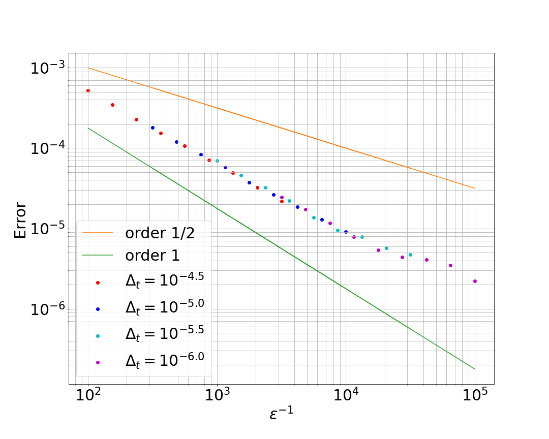
(b) Rate of Convergence

Figure 5: Sensitivity of rate of convergence with respect to changes in $\Delta_{t}$

References

- [1] Florin Avram and Murad S. Taqqu “Probability bounds for M-Skorohod oscillations” In Stochastic Processes and their Applications 33.1, 1989, pp. 63–72
- [2] Patrick Billingsley “Convergence of Probability Measures” John Wiley & Sons, 2013
- [3] Matteo Burzoni and Luciano Campi “Mean field games with absorption and common noise with a model of bank run” In arXiv preprint arXiv:2107.00603, 2021
- [4] René Carmona, François Delarue and Daniel Lacker “Mean field games with common noise” In Annals of Probability 44.6 Institute of Mathematical Statistics, 2016, pp. 3740–3803.
- [5] L. Chayes and G. Swindle “Hydrodynamic limits for one-dimensional particle systems with moving boundaries” In Annals of Probability 24.2 Institute of Mathematical Statistics, 1996, pp. 559–598
- [6] Lincoln Chayes and Inwon C. Kim “A two-sided contracting Stefan problem” In Communications in Partial Differential Equations 33.12 Taylor & Francis, 2008, pp. 2225–2256
- [7] Nikolai N. Chentsov “Weak convergence of stochastic processes whose trajectories have no discontinuities of the second kind and the “heuristic” approach to the Kolmogorov-Smirnov tests” In Theory of Probability & Its Applications 1.1 SIAM, 1956, pp. 140–144
- [8] Christa Cuchiero, Stefan Rigger and Sara Svaluto-Ferro “Propagation of minimality in the supercooled Stefan problem” In The Annals of Applied Probability 33.2, 2023, pp. 1588–1618
- [9] François Delarue, James Inglis, Sylvain Rubenthaler and Etienne Tanré “Particle systems with a singular mean-field self-excitation. Application to neuronal networks” In Stochastic Processes and their Applications 125.6 Elsevier, 2015, pp. 2451–2492
- [10] François Delarue, Sergey Nadtochiy and Mykhaylo Shkolnikov “Global solutions to the supercooled Stefan problem with blow-ups: regularity and uniqueness” In Probability and Mathematical Physics 3.1 Mathematical Sciences Publishers, 2022, pp. 171–213
- [11] Emmanuele DiBenedetto and Avner Friedman “The ill-posed Hele-Shaw model and the Stefan problem for supercooled water” In Transactions of the American Mathematical Society 282.1, 1984, pp. 183–204
- [12] A. Fasano, M. Primicerio and K.. Hadeler “A critical case for the solvability of Stefan-like problems” In Mathematical Methods in the Applied Sciences 5.1 Wiley Online Library, 1983, pp. 84–96
- [13] A. Fasano, M. Primicerio, S.. Howison and J.. Ockendon “On the singularities of one-dimensional Stefan problems with supercooling” In Mathematical Models for Phase Change Problems Springer, 1989, pp. 215–226
- [14] Antonio Fasano and Mario Primicerio “New results on some classical parabolic free-boundary problems” In Quarterly of Applied Mathematics 38.4, 1981, pp. 439–460
- [15] Walter Gautschi “Some elementary inequalities relating to the gamma and incomplete gamma function” In Journal of Mathematics and Physics 38.1-4, 1959, pp. 77–81
- [16] Ben Hambly, Sean Ledger and Andreas Søjmark “A McKean–Vlasov equation with positive feedback and blow-ups” In Annals of Applied Probability 29.4 Institute of Mathematical Statistics, 2019, pp. 2338–2373
- [17] Ben Hambly and Andreas Søjmark “An SPDE model for systemic risk with endogenous contagion” In Finance and Stochastics 23.3 Springer, 2019, pp. 535–594
- [18] S.. Howison, J.. Ockendon and A.. Lacey “Singularity development in moving-boundary problems” In The Quarterly Journal of Mechanics and Applied Mathematics 38.3, 1985, pp. 343–360
- [19] James Inglis and Denis Talay “Mean-field limit of a stochastic particle system smoothly interacting through threshold hitting-times and applications to neural networks with dendritic component” In SIAM Journal on Mathematical Analysis 47.5, 2015, pp. 3884–3916
- [20] Vadim Kaushansky and Christoph Reisinger “Simulation of a simple particle system interacting through hitting times” In Discrete & Continuous Dynamical Systems - B 24.10, 2019, pp. 5481–5502
- [21] Vadim Kaushansky, Christoph Reisinger, Mykhaylo Shkolnikov and Zhuo Qun Song “Convergence of a time-stepping scheme to the free boundary in the supercooled Stefan problem” In The Annals of Applied Probability 33.1, 2023, pp. 274–298
- [22] Hiroshi Kunita “Tightness of probability measures in d ([0, t]; c) and d ([0, t]; d)” In Journal of the Mathematical Society of Japan 38.2, 1986, pp. 309–334
- [23] A.. Lacey and J.. Ockendon “Ill-posed free boundary problems” In Control and Cybernetics 14.275-296, 1985, pp. C432
- [24] Sean Ledger and Andreas Søjmark “At the mercy of the common noise: blow-ups in a conditional McKean–Vlasov problem” In Electronic Journal of Probability 26 Institute of Mathematical StatisticsBernoulli Society, 2021, pp. 1–39
- [25] Sean Ledger and Andreas Søjmark “Uniqueness for contagious McKean–Vlasov systems in the weak feedback regime” In Bulletin of the London Mathematical Society 52.3 Wiley Online Library, 2020, pp. 448–463
- [26] Alexander Lipton, Vadim Kaushansky and Christoph Reisinger “Semi-analytical solution of a McKean–Vlasov equation with feedback through hitting a boundary” In European Journal of Applied Mathematics 32.6 Cambridge University Press, 2021, pp. 1035–1068
- [27] Sergey Nadtochiy and Mykhaylo Shkolnikov “Mean field systems on networks, with singular interaction through hitting times” In The Annals of Probability 48.3, 2020, pp. 1520–1556
- [28] Sergey Nadtochiy and Mykhaylo Shkolnikov “Particle systems with singular interaction through hitting times: application in systemic risk modeling” In The Annals of Applied Probability 29.1 Institute of Mathematical Statistics, 2019, pp. 89–129
- [29] Yu V. Prokhorov “Convergence of random processes and limit theorems in probability theory” In Theory of Probability & Its Applications 1.2 SIAM, 1956, pp. 157–214
- [30] Bernard Sherman “A general one-phase Stefan problem” In Quarterly of Applied Mathematics 28.3, 1970, pp. 377–382
- [31] Joseph Stefan “Über einige Probleme der Theorie der Wärmeleitung” In Sitzungber., Wien, Akad. Mat. Natur 98, 1889, pp. 473–484
- [32] Ward Whitt “Stochastic-Process Limits: An Introduction to Stochastic-Process Limits and Their Application to Queues” Springer Science & Business Media, 2002