Radio multiwavelength analysis of the compact disk CX Tau:
Presence of strong free-free variability or anomalous
microwave emission

Protoplanetary disks emit radiation across a broad range of wavelengths, requiring a multiwavelength approach to fully understand their physical mechanisms and how they form planets. Observations at submillimeter to centimeter wavelengths can provide insights into the thermal emission from dust, free-free emission from ionized gas, and possible gyro-synchrotron emission from the stellar magnetosphere. This work is focused on CX Tau, a ${\sim}0.4\,M_{\odot}$ star with an extended gas emission and a compact and apparently structureless dust disk, with an average millimeter flux compared to Class II sources in Taurus. We present observations from the Karl G. Jansky Very Large Array (VLA) across four bands (between $9.0\text{\,}\mathrm{mm}$ and $6.0\text{\,}\mathrm{cm}$) and combine them with archival data from the Atacama Large Millimeter/submillimeter Array (ALMA), the Submillimeter Array (SMA), and the Plateau de Bure Interferometer (PdBI). This multiwavelength approach allows us to separate the dust continuum from other emissions. After isolating the dust thermal emission, we derived an upper limit of the dust disk extent at $1.3\text{\,}\mathrm{c}\mathrm{m}\mathrm{,}$ which is consistent with theoretical predictions of a radial drift-dominated disk. The centimeter data show a peculiar behavior: deep observations at $6.0\text{\,}\mathrm{cm}$ did not detect the source, while at $1.3\text{\,}\mathrm{c}\mathrm{m}\mathrm{,}$ the flux density is anomalously higher than adjacent bands. Intraband spectral indices suggest a dominant contribution from free-free emission, whereas gyro-synchrotron emission is excluded. To explain these observations, we propose a strong variability among the free-free emission with timescales shorter than a month. Another possible interpretation is the presence of anomalous microwave emission from spinning dust grains.

1 Introduction

Protoplanetary disks are complex systems consisting of gas, dust, and ionized particles surrounding young stars, and they emit radiation over a wide range of wavelengths from radio to X-rays. A multiwavelength approach therefore becomes crucial to understanding the physical mechanisms occurring in disks and explain how they evolve and possibly go on to form planets.

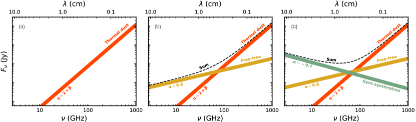
Figure 1: Illustrative plot for the main components in the continuum emission of a typical protoplanetary disk in the wavelength range between the submillimeter to the centimeter. The three panels are described in Sect. 1.

In the last few decades, observations in the submillimeter to centimeter wavelength range revealed different emission mechanisms by analyzing their spectral flux density distributions (e.g., Rodmann et al. 2006; Ricci et al. 2010; Pascucci et al. 2014; Sheehan et al. 2016; Coutens et al. 2019). In this context, a powerful diagnostic able to disentangle the various physical origins of the emission is the spectral index, $\alpha=\log_{10}\left[F_{\nu_{1}}/F_{\nu_{2}}\right]\,/\,\log_{10}[\nu_{1}/\nu_{2}]$, where $F_{\nu_{1}}$ and $F_{\nu_{2}}$ are the flux densities measured in the observing wavelengths, $\nu_{1}$ and $\nu_{2}$, respectively. We summarize the most common cases in Fig. 1, based on the dominant physical mechanism of emission. The first category (panel a) consists of disks in which the thermal emission from dust dominates at all wavelengths. Assuming optically thin emission and Rayleigh-Jeans approximation, dust emission follows a spectral index of $\alpha{\sim}2+\beta$, where $0\lesssim\beta\lesssim 2$ is the dust opacity spectral index and depends on the maximum grain size (see, e.g., Draine 2006; Ricci et al. 2010; Testi et al. 2014; Tazzari et al. 2021). The second category (panel b) includes disks in which dust emission dominates down to a wavelength of a few millimeters, followed by a change in the spectral index due to the contribution of free-free emission at longer wavelengths. Free-free emission originates through the interaction of free electrons with ions in the ionized gas present in the innermost regions of disks or in jets and its spectral index can range from -0.1 to 2.0 in the case of a totally optically thin or optically thick emission, respectively (Ubach et al. 2017). A typical value is $\alpha{\sim}0.6,$ as predicted by the theoretical models of an expanding partially optically thick spherical wind (Panagia & Felli 1975) or a collimated conical jet (Reynolds 1986). Photoevaporative winds can also produce optically thin free-free emission with a spectral index of ${\sim}\,{-}0.1$ (Pascucci et al. 2012), and both jet and wind could coexist (e.g., Macías et al. 2016). Finally, the third category (panel c) includes disks in which a gyro-synchrotron outburst is occurring and dominates at centimeter wavelengths. This non-thermal emission arises from the interaction of electrons with the stellar magnetosphere. Its spectral index depends on the electron energy distribution and it is generally negative with a typical value of $\alpha{\sim}\,{-}0.7$ (Condon & Ransom 2016).

The advantages of detailed multiwavelength analysis to study single protoplanetary disks have been explored in a few recent papers (Carrasco-González et al. 2019 for HL Tau, Macías et al. 2021 for TW Hya, and Guidi et al. 2022 for HD 163296). In this work, we focus on CX Tau. It is a M2.5 star (Luhman 2018) located at a distance from the Sun of $126.5\pm 0.3\,\mathrm{pc}$, as estimated by Bailer-Jones et al. (2021), using Gaia EDR3 (Gaia Collaboration et al. 2021). Simon et al. (2019) measured a dynamical mass of $0.38\pm 0.02\,M_{\odot}$ and Andrews et al. (2013) obtained a stellar bolometric luminosity $L_{\star}=0.38\pm 0.05\,L_{\odot}$ and an effective temperature $T_{\mathrm{eff}}=3475\pm 130\,\mathrm{K}$. The estimated accretion rate is $7.1\times 10^{-10}\,M_{\odot}\ \mathrm{yr}^{-1}$ (Hartmann et al. 1998). From the infrared excess in the SED, Najita et al. (2007) classified the source as a transitional disk, but the presence of an inner cavity has not been detected with high angular resolution observations by Facchini et al. (2019). CX Tau hosts a compact dust disk and an extended gas disk, with a ratio between the gas and dust radii of 5.4 (Facchini et al. 2019), indicating that the disk evolution is dominated by dust radial drift (Weidenschilling 1977). This is in contrast to the majority of disks that show a ratio between the gas and dust radii of ${\sim}2.5$, interpreted by invoking planet formation that is halting dust radial drift (Sanchis et al. 2021, Toci et al. 2021).

CX Tau is an excellent candidate for a thorough multiwavelength analysis for two main reasons. First, it represents a typical protoplanetary disk, due to its small size along with a millimeter flux at the 50th percentile of the flux distribution of Class II disks in Taurus. Second, CX Tau has already been observed by the Atacama Large Millimeter/submillimeter Array (ALMA) in Band 6 ($1.3\text{\,}\mathrm{mm}$) at a high resolution of 0.04” (corresponding to ${\sim}$5\text{\,}\mathrm{au}$$), and the results are presented in Facchini et al. (2019). At this angular resolution, there is no sign of substructures and the data are consistent with a smooth disk model. The authors estimated a total flux density of 9.75 mJy and a radius enclosing 68% of the continuum flux density ($R_{68\%}$) equal to $14\text{\,}\mathrm{au}$. Moreover, they revealed that the brightness radial profile of CX Tau is consistent with the central regions of the profiles of DSHARP disks that are not in a binary system and do not present an inner cavity. Therefore, CX Tau is not a scaled-down version of more extended disks but differs from the latter only for the lack of rings at large radii.

In this work, we present observations from the Karl G. Jansky Very Large Array (VLA) of CX Tau in Ka ($9.0\text{\,}\mathrm{mm}$), K ($1.3\text{\,}\mathrm{cm}$), Ku ($2.0\text{\,}\mathrm{cm}$), and C ($6.0\text{\,}\mathrm{cm}$) bands. Combining these observations with archival data from ALMA in Band 7 ($0.9\text{\,}\mathrm{mm}$) and with values from the literature in the (sub)millimeter, we obtained a multiwavelength view of CX Tau. This paper is organized as follows. Section 2 presents the observations and the procedures we used to reduce and calibrate them, Sect. 3 describes the analysis and the obtained results, and Sect. 4 discusses these findings in light of multiwavelength analyses in general.

2 Observations and data reduction

CX Tau was observed with VLA in the Ka band in B configuration (maximum baseline of $11.1\text{\,}\mathrm{km}$) on 12 October 2020 (VLA Project 20A-373, PI: M. Tazzari) with an on-source integration time of 1.6 hours. The spectral windows covered the range between 29 and $37\text{\,}\mathrm{GHz}$ (corresponding to wavelengths of $8.1-$10.3\text{\,}\mathrm{mm}$$). During the observation, 3C147 was used as bandpass and absolute flux calibrator, J0403+2600 as the pointing calibrator, and J0438+3004 as complex gain (amplitude and phase) calibrator.

Under the same VLA project, CX Tau was observed in the Ku band in C configuration (maximum baseline of $3.4\text{\,}\mathrm{km}$) on 2 and 4 March 2020 for a total on-source integration time of 24 minutes. The bandwidth extended from 12 to $18\text{\,}\mathrm{GHz}$ (wavelengths between 1.7 and $2.5\text{\,}\mathrm{cm}$). The flux and band calibrator was 3C147, the complex gain calibrator was J0431+2037, and both sources were used to calibrate the pointing.

For the C band, we have observations from two different VLA projects. Under project 20A-373, observations were performed in C configuration on 20 February 2020 with a total time on-source of 15 minutes. The wavelength coverage was from 4 to $8\text{\,}\mathrm{GHz}$ ($3.7-$7.5\text{\,}\mathrm{cm}$$). For the calibration, the same sources as for the Ku band data were used. Then, CX Tau was observed again in the C band but with an A configuration (maximum baseline of $36.4\text{\,}\mathrm{km}$) between 9 and 11 January 2021, for a total integration time of 3.8 hours (VLA Project 20B-299, PI: M. Tazzari). Here, 3C147 was used as bandpass and flux calibrator and J0403+2600 as complex gain calibrator.

Observations in the K band were performed more recently, on 9 April 2022 (VLA Project 22A-401, PI: M. Tazzari). The integration time was 15 minutes and the spectral windows ranged from 18.4 to $26.2\text{\,}\mathrm{GHz}$ (wavelengths from 1.1 to $1.6\text{\,}\mathrm{cm}$). 3C147 was employed for the calibration of pointing, bandpass, and flux, while J0403+2600 was the complex gain calibrator.

First, all these observations were calibrated by the VLA pipeline. Then, we performed the self-calibration using the software CASA, version 6.2 (CASA Team et al. 2022). We executed a spectral average on each dataset taking into account the requirements to avoid bandwidth smearing, but did not employ time averaging during the self-calibration. For the imaging, we employed Briggs weighting with robust 1 as the best compromise between signal-to-noise ratio (S/N) and side lobes effects, and the mtmfs deconvolver to properly take into account the relevant bandwidth over observing frequency ratio in VLA data. We performed one round of phase-only self-calibration for the observations in the Ka and Ku bands obtaining improvements in the peak S/N by a factor of 2.3 and 2.9, respectively. For the C-band observation, we kept the observations from the two different configurations separate. In both cases, we executed one round of phase self-calibration always taking as a reference the flux density from the other sources in the field of view, given the lack of a detection for CX Tau emission at this wavelength. We obtained a modest ${\sim}10\%$ increase in the S/N. We placed a particular emphasis on the treatment of the K-band data, carefully checking the calibration executed with the VLA pipeline and performing four rounds of phase-only self-calibration which highly improved the peak S/N by a factor of 7.8 (see Appendix B for details).

In addition to these VLA observations, we also reduced and calibrated the ALMA archival data in Band 7 ($0.9\text{\,}\mathrm{mm}$) from the project 2013.1.00426.S (PI: Yann Boehler) presented in Simon et al. (2017). We performed four rounds of phase-only self-calibration, for an improvement in the peak S/N of 20%.

3 Analysis and results

3.1 Spectral flux density distribution

Figure 2 presents the spectral flux density distribution with all the observations in the submillimeter to centimeter range, including data from VLA, ALMA, the Submillimeter Array (SMA), and the Plateau de Bure Interferometer (PdBI) (Andrews & Williams 2005, Ricci et al. 2010, Piétu et al. 2014, Simon et al. 2017, Facchini et al. 2019). The ALMA and VLA images, along with a table containing properties from all the observations, are given in Appendix A.

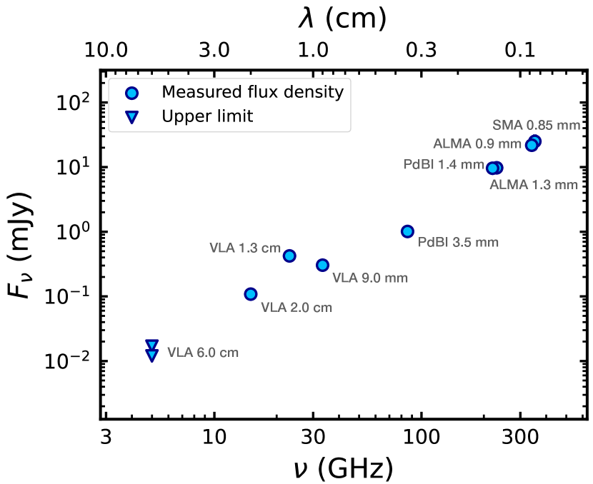
Figure 2: Spectral flux density distribution of CX Tau including data in the submillimeter to centimeter range. For each value of the flux density we report the total uncertainty including the statistical and systematic flux calibration errors. In most cases, the error bars fall within the plotted points. Non-detections are indicated by the upper limits, obtained as the flux from a visibility fit of a central point source plus $2\times\mathrm{RMS}$.

To estimate the integrated flux density and, for the wavelengths where the source is resolved, the radial extent of the dust emission, we performed a characterization in the $uv$-plane using the code galario (Tazzari et al. 2018). We computed the best-fit model using a Markov chain Monte Carlo (MCMC) approach, assuming that the emission is axisymmetric (see Appendix C). The observations with ALMA at $0.9\text{\,}\mathrm{mm}$ are spatially resolved, so we employed a Gaussian profile to model the intensity profile: $I(R)=f_{0}\,\exp{(-R/2\sigma^{2})}$, where $f_{0}$ is a normalization term, $\sigma$ characterizes the Gaussian centered in the disk center, and $R$ is the radial coordinate. The continuum emission in the VLA observations at $9.0\text{\,}\mathrm{mm}$ and $2.0\text{\,}\mathrm{cm}$ are unresolved, so we modeled the disk as a central point source $I(R)=f_{0}\,\delta(R)$, where $\delta(R)$ is the Dirac delta function. To perform this fit for the $2.0\text{\,}\mathrm{cm}$ data, we subtracted the CLEAN model visibilities of an external source in the field of view at an angular distance of ${\sim}$100\text{\,}\arcsec$$ from CX Tau using the CASA task uvsub. In every run, we also fit for the right ascension and declination offsets ($\Delta\mathrm{RA}$, $\Delta\mathrm{Dec}$), but we kept fixed the disk inclination and position angle from the estimates of Facchini et al. (2019) ($\mathrm{inc}=55.1^{\circ}$, $\mathrm{PA}=66.2^{\circ}$), as they were obtained with data that had a higher resolution and sensitivity than all the other observations. In the two 6.0 cm observations, a clear central source was not detected. To estimate a flux density upper limit, we adopted the same procedure as Barenfeld et al. (2016). We employed the CASA task uvmodelfit and fit a central point source to the visibilities of each dataset, after subtracting the other sources in the field of view with uvsub. To this value, we added $2\times\mathrm{RMS}$, so that the upper limit contains the real source flux with a confidence level of 95%. At $1.3\text{\,}\mathrm{cm}$, despite the highest angular resolution available with the VLA at this wavelength (${\sim}$0.1\text{\,}\arcsec$$ corresponding to ${\sim}$13\text{\,}\mathrm{au}$$), the source is dominated by an unresolved component but shows hints of a marginally resolved source. To extract the flux density, we fit these data with a point source, but an attempt to retrieve the radial extent is described in Sect. 3.3. We present all the results of these galario fits in Appendix C.

3.2 Evaluating time variability at centimeter wavelengths

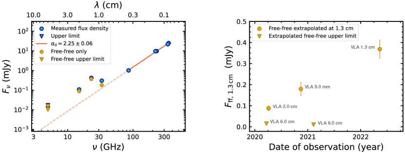
Figure 3: Extraction and time variability of the free-free component. Left panel: Flux density distribution of CX Tau, showing the dust emission fit (orange line) used to extract the free-free only estimates (yellow circles and arrows) from the measured flux densities and upper limits. Right panel: Time variability of extrapolated free-free estimates at 1.3 cm. The extrapolation was performed assuming a free-free spectral index of $0.7\pm 0.1$. The values in the plot are labeled with the observation they came from originally.

Looking at the spectral density distribution in Fig 2, two characteristics appear particularly surprising. First, the two observations at $6.0\text{\,}\mathrm{cm}$ did not detect any emissions, despite the stringent upper limit of $12.0\text{\,}\mathrm{\mu Jy}$ provided by the data taken in A configuration. Second, the emission at $1.3\text{\,}\mathrm{cm}$ is significantly higher than the emissions in the adjacent bands at $9.0\text{\,}\mathrm{mm}$ and $2.0\text{\,}\mathrm{cm}$. In particular, the $1.3\text{\,}\mathrm{cm}$ observation has a flux density higher by a factor of ${\sim}2$ than a power-law fit between the emission at $9.0\text{\,}\mathrm{mm}$ and $2.0\text{\,}\mathrm{cm}$ would suggest. Checking the intraband spectral indices of these three VLA detections resulted for each observation in a value between ${\sim}0.5$ and 1.1 (see Appendix D). This is compatible with the typical value of the free-free spectral index $\alpha{\sim}0.6$ (Panagia & Felli 1975; Reynolds 1986), while excluding contributions from gyro-synchrotron emission that are typically characterized by a negative spectral index. Therefore, we interpret the VLA observations as dominated by free-free emission and explain the non-detections at $6.0\text{\,}\mathrm{cm}$ and the anomalously high emission at $1.3\text{\,}\mathrm{cm}$ as due to the time variability of free-free.

The procedure we applied to evaluate the time variability is summarized in the left panel of Fig. 3. We first assumed that the flux density detected in the observations between $0.9\text{\,}\mathrm{mm}$ and $3.5\text{\,}\mathrm{mm}$ is dominated by dust emission only. Fitting a power-law to these data, we obtained a dust spectral index $\alpha_{\mathrm{d}}=2.25\pm 0.06$ (orange solid line), consistent with partially optically thick dust emission and/or grain growth in the assumption of optically thin emission and Rayleigh-Jeans approximation (Draine 2006). Extrapolating the fit to centimeter wavelengths (orange dashed line) makes it apparent that the flux density from VLA detections diverges from millimeter data, in a way that resembles the behavior in panel b of Fig 1. Then, assuming that VLA detections only have contributions from free-free and dust emission, we obtained the estimates of free-free alone (yellow circles) by subtracting the extrapolation of the dust emission fit from the measured flux densities for the respective observing wavelength. With the intent of comparing the free-free emissions at the same wavelength, we chose $1.3\text{\,}\mathrm{cm}$ as the reference and extrapolated to this wavelength the free-free only estimates at the other VLA bands, assuming a spectral index $\alpha_{\mathrm{ff}}=0.7\pm 0.1$ consistent with the intraband spectral indices of the VLA detections. For the free-free extraction and extrapolation, the two upper limits at $6.0\text{\,}\mathrm{cm}$ are treated in the same way as the detections at $9.0\text{\,}\mathrm{mm}$, $1.3\text{\,}\mathrm{cm}$, and $2.0\text{\,}\mathrm{cm}$. We report in the right panel of Fig. 3 the extrapolated values of the free-free only emission at $1.3\text{\,}\mathrm{cm}$ as a function of the time of their respective observations. There is significant variability both in amplitude and also in time, particularly noticeable by the fact that the first non-detection at $6.0\text{\,}\mathrm{cm}$ and the $2.0\text{\,}\mathrm{cm}$ measurement are separated by ${\sim}2$ weeks. It should be noted that we used a constant spectral index for dust emission at all wavelengths to be conservative. Typically, the dust spectral index steepens at centimeter wavelengths due to grain properties and size distribution (Wilner et al. 2005). In spite of this, a steeper spectral index would not affect the evident variability in the extrapolated free-free emission.

3.3 Relation between dust radius and observing wavelength

Studying the dust radius dependence on observing wavelength provides a useful metric to assess disk evolution. Since different wavelengths are more sensitive to the emission of different dust grain sizes, we expect that the observed disk radius should change with the observing frequency. Specifically, the theoretical prediction by Rosotti et al. (2019) (using dust evolution models that account for grain growth and drift by Birnstiel et al. 2012) suggests that at centimeter wavelengths, probing bigger grains subject to stronger radial drift (Weidenschilling 1977), the extent of a radial-drift-dominated disk should be smaller compared to the radii measured at shorter wavelengths.

For CX Tau, Facchini et al. (2019) at $1.3\text{\,}\mathrm{m}\mathrm{m}$ measured a radius enclosing 68% of the flux density ($R_{68\%}$) of $14.0\pm 0.3\,\mathrm{au}$. From the galario fit with a Gaussian profile of ALMA $0.9\text{\,}\mathrm{mm}$ data, we obtained $R_{68\%}=16.9\pm 0.1\,\mathrm{au}$. The VLA observation with the highest angular resolution is the one in the K band at $1.3\text{\,}\mathrm{cm}$ with a beam of ${\sim}$0.1\text{\,}\arcsec$$. The source is mostly unresolved, but we retrieved an upper limit for the dust size by excluding the noisy visibilities at longer baselines and subtracting the estimate of the unresolved free-free only emission to the real part of all remaining visibilities (see details in Appendix E). Fitting the residual visibilities with galario using a Gaussian profile, we acquired $R_{68\%}=9.2\pm 1.5\,\mathrm{au}$. We interpret this value as an upper limit because the subtraction of a constant value to the real part of all visibilities implies that some unresolved dust emission has possibly been excluded, thereby skewing the inferred extent to a larger size. Figure 4 presents the relation between the measured $R_{68\%}$ (normalized to the value at 0.9 mm) and the observing wavelength for CX Tau compared to the radial drift prediction by Rosotti et al. (2019). The same relation is also shown for AS 209, FT Tau, DR Tau (data from Pérez et al. 2012; Tazzari et al. 2016), and the disks within the survey in Lupus of Tazzari et al. (2021). Unlike the other sources, CX Tau appears consistent with the theoretical prediction for a disk dominated by radial drift. This is in line with the fact that CX Tau is a rare example of a disk whose dust emission is smooth even with high-resolution ALMA observations (another example is PDS 66, Ribas et al. 2023). Moreover, the ratio between the gas and dust radii of 5.4 measured by Facchini et al. (2019) at $1.3\text{\,}\mathrm{mm}$ matches the results from the population synthesis study of Toci et al. (2021) for a Shakura & Sunyaev (1973) disk viscosity value of ${\sim}10^{-3}-10^{-4}$.

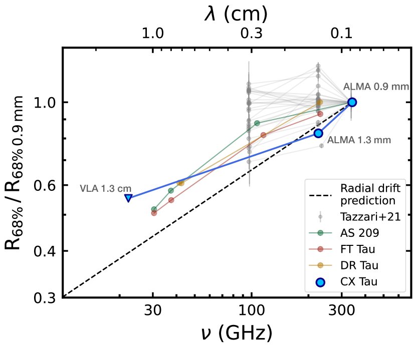
Figure 4: Relation between the measured $R_{68\%}$ (normalized to the value at 0.9 mm) and the observing wavelength for CX Tau, compared with the radial drift prediction by Rosotti et al. (2019) and with the same relation for AS 209, FT Tau, DR Tau (Pérez et al. 2012; Tazzari et al. 2016), and the disks of the Lupus survey by Tazzari et al. (2021).

4 Discussion and conclusions

In this work, we present a multiwavelength view of the compact protoplanetary disk CX Tau in the submillimeter to centimeter range. After a careful subtraction of the contaminant emission, we detected dust thermal continuum at $1.3\text{\,}\mathrm{cm}$, indicating the presence of large grains and the dominance of dust radial drift in the evolution of this disk. This is in line with the observed high ratio between the gas and dust radii consistent with radial drift (Facchini et al. 2019, Sanchis et al. 2021, Toci et al. 2021). Such a scenario implies that dust traps may not be forming within these disks – or, alternatively, the planet formation process is restricted to the inner regions. In either case, CX Tau presents an intriguing example suggesting the need for future observations with higher resolution.

We explain the peculiar scatter of the VLA data in the flux density distribution as the result of a strong time variability of unresolved free-free emission. Free-free emission is known to rarely vary in intensity by more than ${\sim}30\%$ over a timescale of some weeks to a few months (e.g., Sheehan et al. 2016, Coutens et al. 2019). CX Tau, instead, shows a rapid variability of about two weeks associated with a change in intensity by a factor of ${\sim}20$ (see the difference in the extrapolated free-free emission between the detection at 1.3 and the non-detections at $6.0\text{\,}\mathrm{cm}$ in the right panel of Fig. 3). Despite our results, some studies (e.g., Espaillat et al. 2019, 2022) have not reported evidence of variability in Class II sources, so it remains unclear what makes some systems variable (and not others).

Assuming that the free-free emission in CX Tau comes from a jet, we consider the evidence by Anglada et al. (2015) of an almost-linear relationship between the free-free emission of a radio jet and its momentum outflow rate. Thus, the observed variability of a factor of ${\sim}20$ would imply approximately the same level of variability in $\dot{M}_{\mathrm{acc}}$ assuming that the jet velocity and the $\dot{M}_{\mathrm{jet}}/\dot{M}_{\mathrm{acc}}$ do not vary significantly (e.g., Cabrit 2007). Assuming, instead, that the free-free is emitted by a photoevaporative wind, the high state at 1.3 cm would correspond to an ionizing luminosity $\Phi_{\mathrm{EUV}}\sim 10^{40}-10^{41}$ photons $\mathrm{s}^{-1}$ (Pascucci et al. 2012), which is considered typical in Class II sources (Coutens et al. 2019). For variability of the order of a couple of weeks, the medium irradiated by this EUV source must be rather dense to ensure that the recombination timescale is short enough. In particular, the electron density of the ionized gas at sub-au scales would be $n>10^{6}\,\mathrm{cm^{-3}}$ (Hollenbach & Gorti 2009) and this would correspond to a wind mass loss rate of ${\sim}10^{-9}\,M_{\odot}\,\mathrm{yr}^{-1}$ (Hollenbach et al. 1994). Another possible description for the high-intensity observation at $1.3\text{\,}\mathrm{cm}$ could be also a radio flare, a known phenomenon due to the high level of activity in pre-main sequence stars (e.g., Bower et al. 2003, Forbrich et al. 2008, Rivilla et al. 2015 report radio flares from the Orion nebula cluster). However, it should be noticed that radio flares often exhibit a negative or flat spectral index, indicative of non-thermal gyro-synchrotron emission, which is contrary to what we have found. These radio flares are usually associated with X-ray flaring activity. Unfortunately, no X-ray observations of CX Tau are available for comparison. Additionally, the absence of spectra of CX Tau at other wavelengths prevents us from inspecting its accretion properties and supporting the interpretation of free-free variability. All these elements further highlight the peculiarity of the findings in CX Tau and warrant caution when interpreting millimeter and non-simultaneous centimeter wavelength observations when evaluating the strength of a non-dust emission component.

As another potential explanation for the observed behavior, we mention the contribution from anomalous microwave emission (AME), whose presence in protoplanetary disks has been claimed by Greaves et al. (2018). The origin of this emission is uncertain. It is thought to be the effect of electric dipole radiation from nanometric spinning dust grains (Draine & Lazarian 1998), but the carrier is still debated. Greaves et al. (2018) discarded an origin hypothesis from polycyclic aromatic hydrocarbons, in favor of one based on nanodiamonds. The presence of AME would generate a characteristic bump at a wavelength of ${\sim}1$ cm in the spectral flux density distribution (see Fig. 1 in Greaves & Mason 2022) that resembles the trend of CX Tau detections at $0.9\text{\,}\mathrm{mm}$, $1.3\text{\,}\mathrm{cm}$, and $2.0\text{\,}\mathrm{cm}$. Given the uncertainties around this emission mechanism and its properties in protoplanetary disks, simultaneous multiwavelength data are needed to corroborate this scenario.

Appendix A Property table and images from VLA and ALMA observations

Table 1 provides a summary of the datasets used in this work and the derived properties. Figure 5 shows the images from the ALMA and VLA observations of CX Tau, along with a zoomed version of the highest angular resolution observation at $1.3\text{\,}\mathrm{mm}$ from Facchini et al. (2019).

Table 1: Parameters of CX Tau observations at all the frequencies we considered.

Wavelength & Observatory	Observation date	Beam	$F_{\mathrm{tot}}$	RMS	$\Delta F_{stat}$	$\Delta F_{\mathrm{tot}}$	$R_{68\%}$
	(d/m/y)	(arcsec)	(mJy)	(mJy beam-1)	(mJy)	(mJy)	(au)
$0.85\text{\,}\mathrm{mm}$ SMA	02/2004 - 01/2005	${\sim}15$	25.0	6.0	6.0	6.5	-
$0.9\text{\,}\mathrm{mm}$ ALMA Band 7	24/07/2015 23/07/2016	$0.28\times 0.19$	21.8	0.12	0.38	2.2	$16.9\pm 0.1$
$1.3\text{\,}\mathrm{mm}$ ALMA Band 6	C40-5: 05/11/2016 C40-8: 25/09/2017	$0.06\times 0.03$	9.75	0.020	0.12	0.98	$14.0\pm 0.3$
$1.3\text{\,}\mathrm{mm}$ PdBI	12/2010 - 02/2013	$0.6\times 0.4$	9.6	0.2	0.2	0.98	-
$3.5\text{\,}\mathrm{mm}$ PdBI	07-08/2007	${\sim}3-4$	1.01	0.13	0.13	0.16	-
$9.0\text{\,}\mathrm{mm}$ VLA Ka-band	12/10/2020	$0.25\times 0.19$	0.304	$7\times 10^{-3}$	$4\times 10^{-3}$	$31\times 10^{-3}$	-
$1.3\text{\,}\mathrm{cm}$ VLA K-band	09/04/2022	$0.14\times 0.09$	0.423	$10\times 10^{-3}$	$6\times 10^{-3}$	$43\times 10^{-3}$	$<9.2\pm 1.5$
$2.0\text{\,}\mathrm{cm}$ VLA Ku-band	02-04/03/2020	$1.7\times 1.6$	0.108	$3\times 10^{-3}$	$2\times 10^{-3}$	$11\times 10^{-3}$	-
$6.0\text{\,}\mathrm{cm}$ VLA C-band	C conf: 20/02/2020	$4.2\times 3.6$	$<17\times 10^{-3}$	$8\times 10^{-3}$	-	-	-
$6.0\text{\,}\mathrm{cm}$ VLA C-band	A conf: 09-11/01/2021	$0.6\times 0.4$	$<12\times 10^{-3}$	$2\times 10^{-3}$	-	-	-

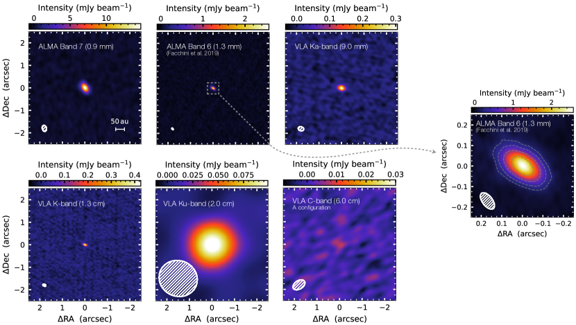
Figure 5: Continuum images of CX Tau from ALMA and VLA observations at different wavelengths, all obtained with Briggs weighting and robust 1. The full width at half maximum (FWHM) of the synthesized beam is indicated by the ellipse in the bottom left corner of each image. The rightmost panel shows a zoomed image of the ALMA 1.3 mm observation from Facchini et al. (2019) which has the highest angular resolution. Contours indicate the [5, 10, 20, 40]$\sigma$ levels.

Appendix B Checks and treatment of the 1.3 cm VLA data

To address the unexpectedly high value of the 1.3 cm VLA data, we present evidence in this section to validate the data collection process and the self-calibration. We carefully examine the gain calibrator J0403+2600 to eliminate the possibility of an incorrect flux transfer that may have influenced the measurement of CX Tau’s flux. The left panel of Fig. 6 presents the image of J0403+2600 from the observation weblog, where nothing seems to be worth of notice. The right panel of Fig. 6 shows the time variability of the flux of the calibrator, comparing the flux value measure in the CX Tau’s execution block to the flux historical values from the source. During the CX Tau observation, the flux value of J0403+2600 is perfectly in line with the historical values. Therefore, the anomalously high value of the 1.3 cm data cannot be explained with an incorrect flux calibration.

We conducted a meticulous four-step phase-only self-calibration procedure. Prior to self-calibration, the RMS was measured at 9.5 $mu$Jy/beam, and the flux density from the CX Tau disk was 70 $mu$Jy, resulting in a peak S/N of 5.1. Throughout the self-calibration process, the RMS remained unchanged, while CX Tau’s flux density steadily increased. The following are the details of each self-calibration step, along with the parameters used for the gaincal task in CASA:

1. We solved for shifts in polarization only with gaintype=’G’, combine=’scan, spw’, and minsnr=3. As a result, the source flux density increased to 100 $mu$Jy.

2. We corrected shifts only between spectral windows with gaintype=’T’, combine=’scan’, and minsnr=3. CX Tau’s flux density reached 160 $mu$Jy.

3. We obtained solutions for both polarization and spectral window shifts with gaintype=’G’, combine=’scan’, and minsnr=3. This caused the flux density to rise to 260 $mu$Jy.

4. We repeated the same command in the fourth step but with a lower threshold for the S/N of the solutions (gaintype=’G’, combine=’scan’, minsnr=2).

At the conclusion of the process, the RMS remained consistent at 9.5 $mu$Jy/beam, while CX Tau’s flux density increased to 420 $mu$Jy, resulting in a peak S/N of 40. It is important to notice that such RMS value is in excellent agreement with the theoretical noise predicted by the VLA exposure calculator which is 9.0 $mu$Jy/beam. From the self-calibration procedure, we can infer that the increase in flux density, coupled with the unchanged RMS, is a result of phase decoherence that dispersed the flux from the central source throughout the field of view. As CX Tau’s flux was not notably high, this effect had minimal impact on the RMS. Consequently, self-calibration successfully gathered and refocused the dispersed flux, leading to an increased integrated flux of the central source.

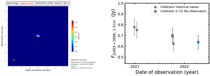
Figure 6: Checks on the gain calibrator J0403+2600 during the CX Tau observation at 1.3 cm. Left panel: Gain calibrator J0403+2600 image at 1.3 cm (K band) from the weblog of the CX Tau observation at the same wavelength. Right panel: Time variability of the 1.3 cm flux density from the gain calibrator J0403+2600.

Appendix C galario fits

To retrieve the flux density, and the radial extent in the case of a resolved observation, we fit the data using the code galario Tazzari et al. (2018). It works by assuming a 1D or 2D model of the emission in the image plane and performing a Fourier transform to obtain the synthetic visibilities at the same $uv$-points of the observations. The best-fit model is found as the one that minimizes the $\chi^{2}$ by sampling the parameter space with an MCMC approach using the emcee package (Foreman-Mackey et al. 2013). We employed uniform priors and the intensity normalization factor $f_{0}$ was sampled logarithmically: $\log_{10}(f_{0}/(\mathrm{Jy/sr}))\in[0,30]$, $\Delta\mathrm{RA}\in[-2,$2\text{\,}\arcsec$]$, $\Delta\mathrm{Dec}\in[-2,$2\text{\,}\arcsec$]$, and, for the fit of ALMA $0.9\text{\,}\mathrm{mm}$ observation, also $\sigma\in[0,$0.2\text{\,}\arcsec$]$. In each run, we used 100 walkers that were well converged after ${\sim}1000$ steps. Corner plots along with deprojected visibilities and best-fit model for data from ALMA Band 7 ($0.9\text{\,}\mathrm{mm}$) and VLA Ka ($9.0\text{\,}\mathrm{mm}$), K ($1.3\text{\,}\mathrm{cm}$), and Ku ($2.0\text{\,}\mathrm{mm}$) bands are shown in Figs. 7, 8, 9, and 10.

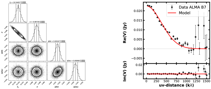
Figure 7: Results of the galario fit with a Gaussian model on ALMA Band 7 ($0.9\text{\,}\mathrm{mm}$) data. Left panel: Corner plot of the MCMC run. Right panel: Recentered and deprojected visibilities binned in 50k$\lambda$ intervals and the best-fit model. Error bars are at $1\sigma$.

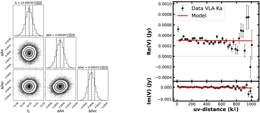
Figure 8: Results of the galario fit with a point source model on the VLA Ka-band ($9.0\text{\,}\mathrm{mm}$) data. Left panel: Corner plot of the MCMC run. Right panel: Recentered and deprojected visibilities binned in 25k$\lambda$ intervals and the best-fit model. Error bars are at $1\sigma$.

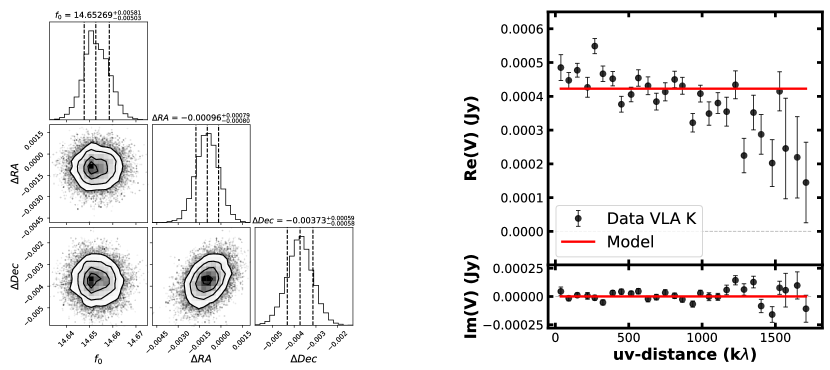
Figure 9: Results of the galario fit with a point source model on the VLA K-band ($1.3\text{\,}\mathrm{cm}$) data. Left panel: Corner plot of the MCMC run. Right panel: Recentered and deprojected visibilities binned in 60k$\lambda$ intervals and the best-fit model. Error bars are at $1\sigma$.

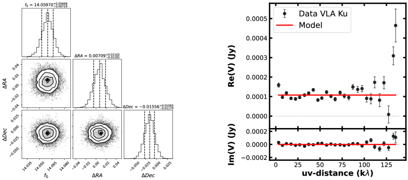
Figure 10: Results of the galario fit with a point source model on the VLA Ku-band ($2.0\text{\,}\mathrm{cm}$) data. Left panel: Corner plot of the MCMC run. Right panel: Recentered and deprojected visibilities binned in 5k$\lambda$ intervals and the best-fit model. Error bars are at $1\sigma$.

Appendix D Intraband spectral indices for VLA observations

To prove that the VLA detections in Ka (9.0 mm), K (1.3 cm), and Ku (2.0 mm) bands are all consistent with free-free emission, despite the high-amplitude variability, we show in Fig. 11 their intraband fluxes. We split each observation into two halves between high and low frequencies and extracted the flux densities. Then, we used a power law to fit the two intensities retrieved from each band and obtained the intraband spectral indices values $\alpha=0.5,\,0.7,\,1.1$ for the data from the Ka, K, and Ku bands, respectively.

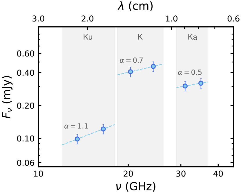
Figure 11: Spectral flux density distribution of CX Tau zoomed in on the VLA data in Ka ($9.0\text{\,}\mathrm{mm}$), K ($1.3\text{\,}\mathrm{cm}$), and Ku ($2.0\text{\,}\mathrm{mm}$) bands. Each observation is split into high and low frequencies and then fitted to obtain the intraband spectral indices reported in the plot.

Appendix E Upper limit for radius estimate from K-band data

The right panel of Fig. 9 shows that the K-band ($1.3\text{\,}\mathrm{cm}$) observation is mostly non-resolved. However, a slight downward trend in the visibility profile is visible, possibly hinting at a resolved component in the data. To extract this component, we first excluded the visibilities at a $uv$-distance greater than 1300k$\lambda$ as they are dominated by noise. Then, we considered only the visibilities in a range of $uv$-distances where they appear the flattest and we chose the interval between 850 and 1300k$\lambda$. We computed the average of the real parts of the visibilities and obtained a flux density of $0.37\text{\,}\mathrm{mJy}$, equivalent to the free-free only estimate obtained by subtracting the extrapolated dust emission from the total flux density value at $1.3\text{\,}\mathrm{cm}$ (indicated by the yellow circle at this wavelength in the left panel of Fig. 3). This procedure is visualized in Fig. 12. We subtracted the computed intensity value to the real parts of the visibilities having a $uv$-distance within 1300k$\lambda$ getting as a result the visibility profile of the resolved dust emission component in the observation. To retrieve a dust size, we fit these visibilities with galario using a Gaussian model profile and the same parameters used in the fit of ALMA $0.9\text{\,}\mathrm{mm}$ data (see Appendix C). The converged fit and the results are shown in Fig 13.

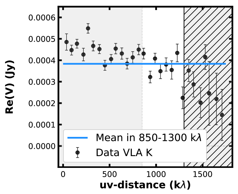
Figure 12: Real part of the visibilities from VLA K-band ($1.3\text{\,}\mathrm{cm}$) data binned in 60k$\lambda$ intervals and overlaid blue line indicating their mean value between 850 and 1300k$\lambda$ (range with white background). The hatched area contains the visibilities with a $uv$-distance greater than 1300k$\lambda$ which have been excluded in the radius evaluation due to high noise.

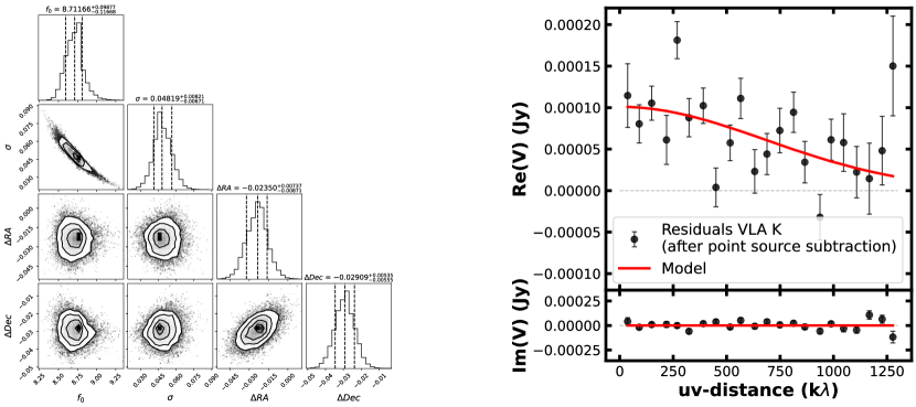
Figure 13: Results of the galario fit with a Gaussian model on VLA K-band ($1.3\text{\,}\mathrm{cm}$) residual data, after subtracting from the real part of the visibilities their mean values in the range of $uv$-distance [850, 1300]k$\lambda$ and neglecting the visibilities over 1300k$\lambda$. Left panel: Corner plot of the MCMC run. Right panel: Recentered and deprojected visibilities binned in 60k$\lambda$ intervals and best-fit model. Error bars are at $1\sigma$.