A Fully Parallelized and Budgeted Multi-level Monte Carlo Method and the Application to Acoustic Waves This work was partly funded by the German Research Foundation (DFG) through an association with the CRC 1173 on Wave Phenomena (Project-ID 258734477). The numerical experiments were executed on the Hochleistungsrechner Karlsruhe (HoReKa) funded by the Ministry of Science, Research and the Arts Baden-Württemberg and by the Federal Ministry of Education and Research.

Abstract

We present a novel variant of the multi-level Monte Carlo method that effectively utilizes a reserved computational budget on a high-performance computing system to minimize the mean squared error. Our approach combines concepts of the continuation multi-level Monte Carlo method with dynamic programming techniques following Bellman’s optimality principle, and a new parallelization strategy based on a single distributed data structure. Additionally, we establish a theoretical bound on the error reduction on a parallel computing cluster and provide empirical evidence that the proposed method adheres to this bound. We implement, test, and benchmark the approach on computationally demanding problems, focusing on its application to acoustic wave propagation in high-dimensional random media.

1 Introduction

Being certain about an outcome of any physical, technical or economical process comes with a cost. This cost manifests in several ways and often includes conducting extensive research, data collection, analysis, and employing sophisticated modeling or simulation techniques. Furthermore, achieving certainty may involve dealing with extremely complex systems in high dimensions and intricate mathematical models which may require the usage of highly advanced and resource-intensive computational technologies.

In this paper, we investigate the computational aspects associated with the cost of certainty, specifically the cost involved in quantifying uncertainty. To address this problem, we propose an integrated framework that combines multi-level Monte Carlo (MLMC), finite element (FE), and dynamic programming (DP) methods. In particular, we introduce a fully parallelized and budgeted variant of the multi-level Monte Carlo method, named as Budgeted MLMC (BMLMC) method. Additionally, we present novel parallelization concepts to handle substantial computational loads.

In recent years, the combination of MLMC and FE methods has been successfully applied to partial differential equations (PDEs) involving random parameters. Notable instances include elliptic PDEs [2, 7, 16, 17, 18, 19, 55] as well as hyperbolic PDEs [6, 31, 40, 41, 42, 43, 44]. The MLMC-FE method provides significant computational efficiency, enabling the achievement of desired accuracy levels while considerably reducing computational requirements compared to a single-level Monte Carlo (MC) method. Despite the existence of alternative uncertainty quantification (UQ) methods, such as stochastic collocation (SC) [3, 4, 46, 45], quasi-Monte Carlo (QMC) techniques [14, 30, 52], as well as various multi-level and multi-index variants described in [34, 35, 38, 54], the MLMC method is a popular choice due to its non-intrusive implementation and the moderate assumptions it imposes on the problem and the employed discretization.

The problems that can be addressed using the method proposed in this paper fall under the domain of forward UQ methods. These problems typically involve solving linear or nonlinear partial differential equations (PDEs) with random input data. In our study, we specifically concentrate on the application of the method to acoustic wave equations in random media. This particular model is of high significance in applications such as seismic imaging and geophysics. As a hyperbolic PDE, it presents unique challenges, including issues related to low regularity, stability conditions, and the handling of high-dimensional random input data.

To tackle this challenge, we developed a high-performance computing (HPC) approach and drew inspiration from previous works such as [44, 57], which address similar problems using MLMC methods. Additionally, we refer to studies such as [11, 20, 24, 36], which focus on different discretization techniques for this particular problem. However, the size of the resulting discrete model, the number of required samples, and the diverse array of solution approaches prompted us to explore new strategies for distributing the computational workload and effectively managing the interplay of all algorithms involved. Consequently, our research and contributions can be summarized by the following three points.

Budgeted multi-level Monte Carlo method

We present a novel budgeted variant of the MLMC method which we call BMLMC method. In the classical MLMC framework described in [7, 18, 17, 27, 28, 55], a desired tolerance for the total root mean squared error (RMSE), denoted as $\epsilon>0$, is selected. Subsequently, a sequence of samples is generated either based on knowledge of the solution’s regularity or by adaptive methods, such as the Continuation MLMC (CMLMC) method [19, 29]. The objective of the adaptive methods is minimizing the overall computational cost while achieving the specified tolerance. In contrast, the BMLMC method is designed to minimize the RMSE and to operate within a given cost budget denoted as $\mathrm{B}>0$. The cost and the budget are specifically measured in units of CPU seconds. A similar approach is also taken by the multi-fidelity method [49] and the unbiased estimation in [51]. This point of view is motivated in the context of this work by two key reasons.

In HPC applications, it is customary to allocate a cost budget to secure a spot in the queue of an HPC cluster. In our notation, this is represented as $\mathrm{B}=\left|\mathcal{P}\right|\cdot\mathrm{T}_{\mathrm{\mathrm{B}}}$, where $\left|\mathcal{P}\right|$ corresponds to the total number of processing units, and $\mathrm{T}_{\mathrm{\mathrm{B}}}$ represents the time budget. Even with a priori knowledge about the solution’s regularity, the convergence rates, the parallelization strategies and the computational infrastructure, determining the tolerance $\epsilon$ that can be achieved with a budget $\mathrm{B}$ remains an NP-hard task. Thus, it is more natural in HPC applications to replace the predefined tolerance $\epsilon$ with a predefined budget $\mathrm{B}$ and allow the method to determine the smallest achievable $\epsilon$ while fully utilizing the budget. This approach aligns with the practical requirements and constraints encountered in HPC scenarios.

Furthermore, employing a budgeted algorithm enables us to address the question of determining the optimal algorithm stack for a given problem. Specifically, we aim to identify the algorithm stack that yields the smallest error while utilizing the same computational resources. We can investigate this question empirically by conducting experiments where various algorithms, e.g. different time stepping methods, are evaluated using an equal budget, and subsequently comparing the resulting error estimates. This empirical analysis allows us to make informed decisions regarding the selection of algorithm combinations that optimize the trade-off between computational resources and the achieved accuracy.

In order to implement our method, we introduce the reserved computational budget as an additional constraint, effectively transforming the problem into a knapsack problem. To solve this knapsack problem, we decompose it into multiple subproblems, each of which is solved under an optimality condition. Specifically, we combine the Continuation MLMC (CMLMC) method [19] with dynamic programming techniques, allowing us to address the problem without any prior knowledge of its specific characteristics or computational complexity. The method proves to be highly robust and performant, and can be widely applied to a general class of PDEs in conjunction with the proposed parallelization strategy.

Parallelization Strategy

Parallelization is an omnipresent challenge in various applications, including manufacturing, logistics, and computer networks. The load distribution of MLMC methods has already been addressed in prior work, such as [5, 25, 53, 56]. However, our parallelization in this study offers a distinguishing feature compared to most of the previous work by being done on a single distributed data structure. This technical choice allows for a more efficient and adaptable load distribution.

In our proposed parallelization scheme, we leverage a multi-mesh parallelism on distributed memory, which can be applied not only to arbitrary FE spaces but also to other non-intrusive UQ algorithms beyond MLMC. The key idea is to assemble large algebraic systems on distributed memory across multiple computing nodes, while dynamically adapting the system’s structure based on the number of samples that need to be computed. This integrated approach seamlessly combines FE with UQ methods, resulting in a highly efficient implementation that fully exploits hardware capabilities without compromising the non-intrusive nature of UQ methods. We refer to this parallelization strategy throughout the paper as multi-sample finite element method (MS-FEM).

By adopting this parallelization strategy, we achieve a highly adaptive and hardware proximal implementation, providing significant computational benefits by minimizing the communication overhead and processor idling. In summary, our parallelization approach offers a novel perspective on distributing computational load and demonstrates its effectiveness in enhancing the performance of UQ algorithms, including the MLMC method.

Numerical Experiments and Software

Lastly, this paper provides a concise insight into the developed software, M++ [59], along with a range of automated numerical experiments. An essential aspect of our implementation is its flexibility, as the methodology can be seamlessly integrated with arbitrary FE and other non-intrusive UQ methods. Consequently, our approach allows for the unified application of these methods to elliptic, parabolic, and hyperbolic PDEs [8, 9], although our focus in this paper is specifically on the application of the BMLMC method to the acoustic wave equation.

It is worth noting that the empirical investigations concerning the algorithm stack have been meticulously conducted using a fully automated approach via a continuous delivery pipeline, ensuring the reproducibility and potential improvement of the presented results. In particular, we describe experiments performed within our framework that encompass the parallelization, model assessment, and methodology evaluation.

Outline

The paper is structured as follows. In Section 2 we establish the notation, state the underlying assumptions, and present the classical MLMC method. Subsequently, we derive the BMLMC method using dynamic programming techniques. Notably, we also demonstrate in this section that any parallel and adaptive implementation of an MLMC method inherently contains an error contribution that cannot be eliminated by increasing the number of processing units. Section 2 is designed to be independent of the specific application, making it applicable to other problems as well. In Section 3, we discuss details of the multi-sample finite element method (MS-FEM), which represents an ideal fit for the requirements of the BMLMC method, offering a highly adaptive and efficient parallelization strategy. We provide a explanation of how we define a multi-sample discontinuous Galerkin (dG) finite element space, which serves as the basis for the subsequent discussion on the discretization of the acoustic wave equation under uncertainty in Section 4. Specifically, we introduce a semi-discrete dG system solved with implicit time-stepping methods in the time domain. Section 5 presents numerical results achieved using the proposed framework. We conclude with a comprehensive discussion and an outlook on further work in Section 6.

2 A Budgeted Multi-level Monte Carlo Method

In this section, we present the budgeted multi-level Monte Carlo (BMLMC) method along with novel approaches for determining the optimal load distribution among a given set of processing units. We begin by establishing the notation and outlining the main assumptions on the stochastic model in Section 2.1. Next, in Section 2.2, we provide an overview of the classical multi-level Monte Carlo method [27, 28]. Section 2.3 focuses on implementation techniques [19, 29] that are utilized in conjunction with dynamic programming (DP) to develop the BMLMC method, as described in Section 2.4. Finally, in Section 2.5, we explain the resulting algorithm as a distributed state machine, leveraging adaptive parallelization techniques and show that the error of any parallel and adaptive implementation of the MLMC method obeys a bound with respect to the computing time and the amount of processing units.

2.1 Assumptions and Notation

In the following, we consider a bounded polygonal domain $\mathcal{D}\subset\mathbb{R}^{D}$ with spatial dimension $D\in\left\{1,2,3\right\}$, and a probability space $(\Omega,\mathcal{F},\mathbb{P})$. We are interested in solving PDEs with uncertainly determined input data, i.e., models of the form $\mathcal{L}(\omega,\mathbf{x})\mathbf{u}(\omega,\mathbf{x})=\mathbf{b}(\omega,\mathbf{x})$, where $\omega\in\Omega$ corresponds to a specific outcome in the probability space and $\mathbf{u}(\omega,\mathbf{x})$ represents the solution of the PDE at spatial location $\mathbf{x}\in\mathcal{D}$. The differential operator $\mathcal{L}(\omega,\mathbf{x})$ depends on the input data and acts on the solution $\mathbf{u}(\omega,\mathbf{x})$, while $\mathbf{b}(\omega,\mathbf{x})$ is a forcing term on the PDE. Later in this work, we also consider time dependent PDE models, which however, relax to the above formulation for a fixed time point. Thereby, the time dependence is neglected throughout this section. For each $\omega\in\Omega$, the solution lies in a separable Hilbert space $V$. Additionally, we consider a bounded functional $\mathrm{Q}(\omega)\coloneqq\mathrm{Q}(\mathbf{u}(\omega,\mathbf{x}))$ that represents a quantity of interest (QoI) of the solution.

As a start, we consider the objective of the method as to estimate the expected value of $\mathrm{Q}$ with a prescribed level of accuracy by approximating the PDE using a FE solution $\mathbf{u}_{\ell}(\omega)\in V_{\ell}$ and employing an MC method to approximate the expectation. In this context, $V_{\ell}$ represents a discrete FE space at level $\ell$ and $\mathbf{u}_{\ell}(\omega,\mathbf{x})$ solves the discrete problem $\mathcal{L}_{\ell}(\omega,\mathbf{x})\mathbf{u}_{\ell}(\omega,\mathbf{x})=\mathbf{b}_{\ell}(\omega,\mathbf{x})$. A specific study of such a system is given in Section 4 in form of the acoustic wave equation discretized with non-conforming dG elements. Furthermore, we denote by $\mathrm{Q}_{\ell}(\omega)\coloneqq\mathrm{Q}_{\ell}(\mathbf{u}_{\ell}(\omega,\mathbf{x}))$ the quantity of interest (QoI) defined on $V_{\ell}$ and give samples the index $m$, i.e., $\mathbf{u}_{\ell}(\omega^{(m)},\mathbf{x})$ represents the FE solution computed using input data corresponding to $\omega^{(m)}$. To numerically represent the input, we make the following assumption.

We rely on the finite dimensional noise assumption (FDNA): the space of outcomes $\Xi$ of any random field $\mathbf{Y}\colon\Omega\times\mathcal{D}\rightarrow\Xi$ is of finite dimension $K$, i.e., any sample can be represented by a vector $\mathbf{y}^{(m)}=(y_{1},\dots,y_{K})^{\top}\in\Xi\subset\mathbb{R}^{K}$.

By the FDNA, we can express samples of the input data by the vector $\mathbf{y}^{(m)}\in\mathbb{R}^{K}$, so that we simply write $\mathbf{u}_{\ell}^{(m)}\coloneqq\mathbf{u}_{\ell}(\mathbf{y}^{(m)},\mathbf{x})$ and $\mathrm{Q}_{\ell}^{(m)}\coloneqq\mathrm{Q}_{\ell}(\mathbf{y}^{(m)})$.

A Monte Carlo method for a FE solution estimates the expected value of a QoI

(1) $$\mathbb{E}[\mathrm{Q}]\coloneqq\int_{\Omega}\mathrm{Q}(\omega)\mathrm{d}\mathbb{P}\approx\frac{1}{M}\sum_{m=1}^{M}\mathrm{Q}_{\ell}(\mathbf{y}^{(m)})\eqqcolon\widehat{\mathrm{Q}}_{\ell}\,,$$

depending on independent and identically distributed (iid) samples $\mathbf{y}^{(m)}\in\Xi\subset\mathbb{R}^{K}$ drawn from the distribution of the input data. Computing $\mathrm{Q}_{\ell}(\mathbf{y}^{(m)})$ requires to solve a PDE with a FE method and thereby is a costly and inexact evaluation admitting a discretization error $\mathrm{err}_{\text{disc}}$. Thus, estimating the expected value comes with an estimator bias induced by the FE method giving a mean squared error (MSE)

(2) $$\mathrm{err}_{\mathrm{MSE}}=\mathbb{E}\left[\left(\widehat{{\mathrm{Q}}}_{\ell}-\mathbb{E}[{\mathrm{Q}}]\right)^{2}\right]=\underbrace{M^{-1}\mathbb{V}[{\mathrm{Q}}_{\ell}]}_{\text{Estimator variance}}+\quad{\underbrace{\mathbb{E}[{\mathrm{Q}}_{\ell}-{\mathrm{Q}}]}_{\text{Bias}}}^{2},$$

where $\mathbb{V}[{\mathrm{Q}}_{\ell}]$ is the variance of the random variable $\mathrm{Q}_{\ell}$ and the corresponding root mean squared error (RMSE) is given by $\mathrm{err}_{\mathrm{RMSE}}=\sqrt{\mathrm{err}_{\mathrm{MSE}}}$. To link the admitted error and the computational cost, we introduce the following definition of a cost-measure.

Definition 2.1 ($\epsilon$-time, $\epsilon$-cost and cost-measure).

For given $\epsilon>0$, the computing time to achieve a root mean squared error $\mathrm{err}_{\mathrm{RMSE}}\leq\epsilon$ is the $\epsilon$-time $\mathrm{T}_{\epsilon}$. The $\epsilon$-cost $\mathrm{C}_{\epsilon}=\left|\mathcal{P}\right|\cdot\mathrm{T}_{\epsilon}$ is the corresponding computational cost on a parallel machine, where $\left|\mathcal{P}\right|$ is the total count of involved processing units.

On a serial machine the $\epsilon$-cost simplifies to $\mathrm{C}_{\epsilon,\mathrm{s}}=\mathrm{T}_{\epsilon}$. Since the classical theory of MLMC methods does not consider parallel machines, the methods in subsections 2.2–2.3 are formulated for a serial $\epsilon$-cost.

Clearly to bound (2) and the total computational cost, we have to assume that we can control the FE error with respect to the discretization parameter $h_{\ell}$ and that the computational cost to evaluate the FE solution for a single sample $\mathrm{C}\left({\mathrm{Q}}_{\ell}(\mathbf{y}^{(m)})\right)$ is finite. Combined with the third assumption given below, we can express a bound for the total computational cost of the MLMC method with respect to the target RMSE $\epsilon$ in the next section.

Suppose the approximation scheme to compute $\mathrm{Q}_{\ell}$ satisfies

(3) $$\left|\mathbb{E}[{\mathrm{Q}}_{\ell}-\mathrm{Q}]\right| \leq c_{\alpha}h_{\ell}^{\alpha}$$

(4) $$\mathbb{V}[{\mathrm{Q}}_{\ell}-{\mathrm{Q}}_{\ell-1}] \leq c_{\beta}h_{\ell}^{\beta}$$

(5) $$\mathrm{C}\left({\mathrm{Q}}_{\ell}(\mathbf{y}^{(m)})\right) \leq c_{\gamma}h_{\ell}^{-\gamma}$$

with $\alpha,\beta,\gamma>0$ and $c_{\alpha},c_{\beta},c_{\gamma}>0$ independently on $\ell$.

2.2 Introduction to Multi-level Monte Carlo methods

The underlying idea of the MLMC method is to construct a model hierarchy for the imposed problem. In FE applications, this can be done with nested meshes $\{\mathcal{M}_{\ell}\}_{\ell=0}^{L}$ with decreasing mesh widths, e.g. $h_{\ell}=2^{-\ell}h_{0}$, for the discretization on level $\ell=0,\dots,L$. The goal is to reduce the number of evaluations of the model on the finest level as much as possible and to minimize the overall estimator variance. For a fixed finest level $L$, the expected value of $\mathrm{Q}_{L}$ can be written as a telescoping sum over the levels

(6) $$\mathbb{E}[{\mathrm{Q}}_{L}]=\mathbb{E}[{\mathrm{Q}}_{0}]+\sum_{\ell=1}^{L}\mathbb{E}[{\mathrm{Q}}_{\ell}-{\mathrm{Q}}_{\ell-1}]=\sum_{\ell=0}^{L}\mathbb{E}[\mathrm{Y}_{\ell}]\,,\quad\mathrm{Y}_{0}\coloneqq{\mathrm{Q}}_{0}\,,\quad\mathrm{Y}_{\ell}\coloneqq{\mathrm{Q}}_{\ell}-{\mathrm{Q}}_{\ell-1}\,.$$

Each expected value of $\mathrm{Y}_{\ell}$ in the telescoping sum is now estimated individually with a MC method, resulting in the MLMC estimator

(7) $$\widehat{{\mathrm{Q}}}^{\text{MLMC}}_{\{M_{\ell}\}_{\ell=0}^{L}}=\sum_{\ell=0}^{L}\widehat{\mathrm{Y}}_{\ell}\,,\qquad\widehat{\mathrm{Y}}_{\ell}=\frac{1}{M_{\ell}}\sum_{m=1}^{M_{\ell}}\mathrm{Y}_{\ell}(\mathbf{y}^{(m)})\,,$$

where $\{M_{\ell}\}_{\ell=0}^{L}$ denotes a sequence for the number of samples on each level. It is important that every $\mathrm{Y}_{\ell}(\mathbf{y}^{(m)})={\mathrm{Q}}_{\ell}(\mathbf{y}^{(m)})-{\mathrm{Q}}_{\ell-1}(\mathbf{y}^{(m)})$ uses the same sample $\mathbf{y}^{(m)}\in\Xi$ for two different meshes. Since all the expected values $\mathbb{E}[\mathrm{Y}_{\ell}]$ are estimated independently, the variance of the MLMC method can be quantified on each level individually and with this, we obtain for the mean squared error

(8) $$\mathrm{err}_{\mathrm{MSE}}\left(\widehat{{\mathrm{Q}}}^{\mathrm{MLMC}}_{\{M_{\ell}\}_{\ell=0}^{L}}\right)=\underbrace{\sum_{\ell=0}^{L}\frac{1}{M_{\ell}}\mathbb{V}[\mathrm{Y}_{\ell}]}_{\text{Estimator variance}}+\,\,\,{\underbrace{\mathbb{E}[{\mathrm{Q}}_{L}-{\mathrm{Q}}]}_{\text{Bias}}}^{2}\,,$$

cf. [18]. Assuming we want to achieve a MSE of $\epsilon^{2}$, i.e., an RMSE tolerance of $\epsilon$, we can reach this accuracy with $\theta\in(0,1)$, if

$$\mathbb{E}[{\mathrm{Q}}_{L}-{\mathrm{Q}}]^{2}<(1-\theta)\epsilon^{2}\quad\text{and}\quad\mathbb{V}\left[\widehat{{\mathrm{Q}}}^{\text{MLMC}}_{\{M_{\ell}\}_{\ell=0}^{L}}\right]<\theta\epsilon^{2}.$$

The parameter $\theta$ can thereby be used to tune the variance bias trade-off in order to favor the minimization of one term over the other. Numerical experiments have shown that for our particular application $\theta=0.5$ is a sufficient choice [8].

Quantitatively, the computational cost of the method is given by

(9) $$\mathrm{C}\left(\widehat{{\mathrm{Q}}}^{\text{MLMC}}_{\{M_{\ell}\}_{\ell=0}^{L}}\right)=\sum_{\ell=0}^{L}\sum_{m=1}^{M_{\ell}}\mathrm{C}_{\ell}(\mathbf{y}^{(m)})=\sum_{\ell=0}^{L}M_{\ell}\widehat{\mathrm{C}}_{\ell}\,,\quad\widehat{\mathrm{C}}_{\ell}=\frac{1}{M_{\ell}}\sum_{m=1}^{M_{\ell}}\mathrm{C}_{\ell}(\mathbf{y}^{(m)})\,,$$

where $\widehat{\mathrm{C}}_{\ell}$ is the sample mean of the cost. We now want to find the optimal sequence of samples $\{M_{\ell}\}_{\ell=0}^{L}$, such that the estimator cost is minimized while achieving an MSE tolerance of $\epsilon^{2}$, cf. [29]. By presetting the MSE tolerance, we can also deduce from (3) the highest level $L$ since the estimator bias has to be smaller than $(1-\theta)\epsilon^{2}$. Thereby, it is sufficient to minimize the estimator cost while achieving an estimator variance of $\theta\epsilon^{2}$, i.e., we search for $\{M_{\ell}\}_{\ell=0}^{L}$ solving

(10) $$\min_{\{M_{\ell}\}_{\ell=0}^{L}}\quad\mathrm{C}\left(\widehat{{\mathrm{Q}}}^{\text{MLMC}}_{\{M_{\ell}\}_{\ell=0}^{L}}\right)\quad\text{s.t.}\quad\sum_{\ell=0}^{L}M_{\ell}^{-1}\mathbb{V}[\mathrm{Y}_{\ell}]=\theta{\epsilon^{2}}.$$

By treating each $M_{\ell}$ as a continuous variable, the solution to this optimization problem is given by

(11) $$M_{\ell}^{\mathrm{opt}}=\left\lceil\left({\sqrt{\theta}\epsilon}\right)^{-2}\sqrt{\frac{\mathbb{V}[\mathrm{Y}_{\ell}]}{\widehat{\mathrm{C}}_{\ell}}}\left(\sum_{\ell^{\prime}=0}^{L}\sqrt{\mathbb{V}[\mathrm{Y}_{\ell^{\prime}}]\widehat{\mathrm{C}}_{\ell^{\prime}}}\right)\right\rceil\quad\text{for}\quad\ell=0,\dots,L.$$

We lastly restate the $\epsilon$-cost theorem of the MLMC method in the form given in [18, 27]:

Theorem 2.2 (Bounded $\epsilon$-cost of the MLMC method).

Suppose assumption 2.1 is fulfilled with some positive rates $\alpha,\beta,\gamma>0$ with $\alpha\geq\tfrac{1}{2}\min\left\{\beta,\gamma\right\}$ and $c_{\alpha},c_{\beta},c_{\gamma}>0$ independent of $h_{\ell}$. Then for any $0<\epsilon<\mathrm{e}^{-1}$, there exists a maximum level $L\in\mathbb{N}$ and a sequence of samples $\{M_{\ell}\}_{\ell=0}^{L}$ such that

$${\mathrm{err}_{\mathrm{RMSE}}}\left(\widehat{{\mathrm{Q}}}^{\mathrm{MLMC}}_{\{M_{\ell}\}_{\ell=0}^{L}}\right)<\epsilon\qquad\text{with}\qquad\mathrm{C}_{\epsilon}\left(\widehat{{\mathrm{Q}}}^{\mathrm{MLMC}}_{\{M_{\ell}\}_{\ell=0}^{L}}\right){\lesssim}\begin{cases}\epsilon^{-2}&\beta>\gamma\,,\\ \epsilon^{-2}\log(\epsilon)^{2}&\beta=\gamma\,,\\ \epsilon^{-2-(\gamma-\beta)/\alpha}&\beta<\gamma\,.\end{cases}$$

with $\lesssim$ denoting that the left hand side obeys an upper bound given by the right hand side up to some hidden constant.

2.3 Implementation Techniques

Implementing the MLMC method with on-the-fly estimation of Section 2.1 is well described in [29] and shortly recalled to commit to our notation. This includes a way to find the optimal sequence $\{M_{\ell}\}_{\ell=0}^{L}$ and the highest level $L$ during runtime. Choosing $M_{\ell}^{\mathrm{opt}}$ by (11) requires estimates for the variance $\mathbb{V}[\mathrm{Y}_{\ell}]$ and the sample mean of the cost $\widehat{\mathrm{C}}_{\ell}$, which are unknown a priori. The idea is to perform the MLMC method with an initial sequence $\{M_{\ell}^{\text{init}}\}_{\ell=0}^{L_{\text{init}}}$ to get first estimates for the sample mean of the cost $\widehat{\mathrm{C}}_{\ell}$ and the variance $\mathbb{V}[\mathrm{Y}_{\ell}]$ by the sample variance estimator

(12) $$s_{\mathrm{Y}_{\ell}}^{2}=\frac{1}{M_{\ell}-1}S_{\mathrm{Y}_{\ell},2}\quad\text{with}\quad S_{\mathrm{Y}_{\ell},2}=\sum_{m=1}^{M_{\ell}}\big{(}\mathrm{Y}_{\ell}^{(m)}-\widehat{\mathrm{Y}}_{\ell}\big{)}^{2}\,.$$

From these initial estimates on, the MLMC method is executed until the target RMSE $\epsilon$ is reached by continuously updating the sample statistics. Hence, the amount of samples accumulates and the required amount is given by ${\vartriangle}M_{\ell}\coloneqq\max\{\widehat{M}_{\ell}^{\text{opt}}-M_{\ell},\,0\}$ with the optimal sample amount based on the estimates

(13) $$\widehat{M}_{\ell}^{\text{opt}}=\left\lceil\left(\sqrt{\theta}\epsilon\right)^{-2}\sqrt{\frac{s^{2}_{\mathrm{Y}_{\ell}}}{\widehat{\mathrm{C}}_{\ell}}}\left(\sum_{\ell^{\prime}=0}^{L}\sqrt{s^{2}_{\mathrm{Y}_{\ell^{\prime}}}\widehat{\mathrm{C}}_{\ell^{\prime}}}\right)\right\rceil\quad\text{for}\quad\ell=0,\dots,L\,.$$

With assumption (3) and the geometric sum, an estimate for the bias is given by

(14) $$\widehat{\mathrm{err}}_{\text{disc}}=\max\left\{\frac{\widehat{\mathrm{Y}}_{\ell}}{2^{\widehat{\alpha}}-1}2^{-{\widehat{\alpha}}(L-\ell)}\colon\ell=1,\dots,L\right\},$$

which also incorporates lower levels for robustness of the estimate, cf. [29], and uses an approximation for ${{\alpha}}$ by fitting the data $\{\widehat{\mathrm{Y}}_{\ell}\}_{\ell=0}^{L}$ to assumption (3)

(15) $$\min_{(\widehat{\alpha},\,\widehat{c}_{\alpha})}\quad\sum_{\ell=1}^{L}\Big{(}\log_{2}\widehat{\mathrm{Y}}_{\ell}+\widehat{\alpha}\ell-\widehat{c}_{\alpha}\Big{)}^{2}\,.$$

This gives the estimates $\widehat{\alpha}$ and $\widehat{c}_{\alpha}$ for the rate $\alpha$ and the constant $c_{\alpha}$ which can be done in a similar way for $(\gamma,c_{\gamma})$ and $(\beta,c_{\beta})$. The estimator variance of the MLMC method is approximated with the sample variance by

$$\widehat{\mathrm{err}}_{\text{input}}=\sum_{\ell=0}^{L}\frac{1}{M_{\ell}}s^{2}_{\mathrm{Y}_{\ell}}$$

and, finally, an estimate for the MSE can be computed with

$$\widehat{\mathrm{err}}_{\text{MSE}}=\widehat{\mathrm{err}}_{\text{input}}+\widehat{\mathrm{err}}_{\text{disc}}^{2}\,.$$

The above techniques are further refined by the CMLMC method [19], also applied in [39, 50]. The central idea is to create a sequence $\epsilon_{\texttt{i}}$ with $\epsilon_{\texttt{i}}\rightarrow\epsilon_{\min}>0$ and by doing so, the above estimates and the required number of samples $\{M_{\texttt{i},\ell}\}_{\ell=0}^{L_{\texttt{i}}}$ are continuously updated for each new tolerance. This idea is now extended with an additional constraint on the total cost, i.e., a budget, giving the budgeted MLMC method.

2.4 Budgeted Multi-level Monte Carlo

In large HPC systems, the workload managers require to reserve computational budget $\mathrm{B}\coloneqq\left|\mathcal{P}\right|\cdot\mathrm{T}_{\mathrm{\mathrm{B}}}$ to initiate a job on the cluster. Therefore, we define an execution of a method on a computing cluster as feasible, if the method is capable of fully utilizing the computational budget without exceeding it. In light of this, we adapt the perspective of Theorem 2.2. The final implementation will contain certain parts of the algorithm which can be parallelized, while others cannot. We denote $\lambda_{\mathrm{p}}\in[0,1]$ as the parallelization constant, representing the portion of the implemented algorithm that is executed in parallel on $\left|\mathcal{P}\right|$ units.

Proposition 2.3 (Convergence of a parallelized BMLMC method).

For a feasible execution of the budgeted method by a parallel implementation, the estimate for the error splits up into two parts

(16) $$\epsilon\lesssim\underbrace{(1-\lambda_{\mathrm{p}})\cdot\mathrm{T}_{\mathrm{\mathrm{B}}}^{-\delta}}_{\eqqcolon\epsilon_{\mathrm{s}}}+\underbrace{\lambda_{\mathrm{p}}(\left|\mathcal{P}\right|\cdot\mathrm{T}_{\mathrm{\mathrm{B}}})^{-\delta}}_{\eqqcolon\epsilon_{\mathrm{p}}}\quad\text{with}\quad\delta=\begin{cases}\hskip 17.07182pt\frac{1}{2}&\beta>\gamma\\ \frac{\alpha}{2\alpha+(\gamma-\beta)}&\beta<\gamma\end{cases}$$

depending on the parallization constant $\lambda_{\mathrm{p}}\in[0,1]$.

For the proof we refer to Section 2.5, here we only comment on the case $\lambda_{\mathrm{p}}=1$ when a perfectly parallel implementation can be realized. Then, in case of a feasible run, the final $\epsilon$-cost equals the budget, and the estimate

(17) $$\epsilon\lesssim\mathrm{B}^{-\delta}=\begin{cases}\mathrm{B}^{-1/2}&\beta>\gamma\\ \mathrm{B}^{-\alpha/(2\alpha+(\gamma-\beta))}&\beta<\gamma\end{cases}$$

simply follows by inverting Theorem 2.2. Similar results can be found e.g. in [37, 44] where the word work was used instead of budget. The case $\beta=\gamma$ is neglected for the sake of a leaner representation and since it has no practical relevance if the cost is measured in units of CPU seconds.

This result does not tell us how to utilize the budget. Thereby, the new algorithmic challenge is to find the best way to invest $\mathrm{B}$, such that we minimize the error. Formally, this is expressed by a knapsack problem:

Problem 2.4 (MLMC Knapsack).

Find $L$ and $\{M_{\ell}\}_{\ell=0}^{L}$, such that the MSE is minimized while staying within the cost budget $\mathrm{B}$, i.e.,

(18a) $$\min_{(L,\{M_{\ell}\}_{\ell=0}^{L})}\quad \mathrm{err}_{\mathrm{MSE}}=\sum_{\ell=0}^{L}\frac{1}{M_{\ell}}\mathbb{V}[\mathrm{Y}_{\ell}]+\big{(}\mathbb{E}[{\mathrm{Q}}_{L}-{\mathrm{Q}}]\big{)}^{2}$$

(18b) s.t. $$\sum_{\ell=0}^{L}\sum_{m=1}^{M_{\ell}}\mathrm{C}_{\ell}(\mathbf{y}^{(m)})\leq\mathrm{B}.$$

We remark the change of perspective to (10). The objective now is to minimize the complete MSE including the bias, while the constraint is given by the computational budget. Knapsack problems, in general, are combinatorial optimization problems and often arise while searching for the optimal allocation of resources, e.g., in manufacturing, in computer networks or in financial models. These integer optimization problems are NP-hard and require effective algorithms often designed with dynamic programming (DP) techniques [12, 13]. The key idea of DP is to split up the initial problem into overlapping subproblems and solve them recursively with some optimal policy, while reusing memoized results stored in a suitable data structure.

Now, the goal is to derive an algorithm satisfying Bellman’s optimality condition of DP, i.e., an algorithm finding a sequence of optimal actions, such that at each state an objective value is maximized. To do so, we have to construct a reward/pay-off function which describes in each state the reward/pay-off for the maximization, if a certain action is taken. For the construction of a suitable reward function, we recognize that we do not know the exact quantities in (18a) and (18b). The following optimization problem is still NP-hard but at least exclusively contains computable quantities.

Problem 2.5 (Approximated MLMC Knapsack).

Find $L$ and the sequence $\{M_{\ell}\}_{\ell=0}^{L}$, such that the estimated MSE is minimized, while staying within the cost budget $\mathrm{B}$, i.e.,

(19a) $$\min_{(L,\{M_{\ell}\}_{\ell=0}^{L})}\quad \widehat{\mathrm{err}}_{\mathrm{MSE}}=\sum_{\ell=0}^{L}\frac{1}{M_{\ell}}s^{2}_{\mathrm{Y}_{\ell}}+\widehat{\mathrm{err}}_{\mathrm{disc}}^{2}$$

(19b) s.t. $$\sum_{\ell=0}^{L}M_{\ell}\widehat{\mathrm{C}}_{\ell}\leq\mathrm{B}\,,$$

where $\widehat{\mathrm{err}}_{\mathrm{disc}}$ is computed with (14) and the sample variance $s_{\mathrm{Y}_{\ell}}^{2}$ by (12).

The idea is to identify the MSE as the value we try to optimize and to split up the initial problem into several estimation rounds with a decreasing sequence of tolerances $\epsilon_{\texttt{i}}$ as in the CMLMC method [19]. This creates subsequent optimization problems where each solution yields some reward to the total optimization. To this end, we equip all quantities of Section 2.3 with an index i. In the following, we motivate the existence of a pay-off/reward function depending on the chosen action $\epsilon_{\texttt{i}}$, and the current state of the simulation, i.e., the collected data up to $\texttt{i}-1$.

Suppose we are in estimation round i and $M_{0,\ell}^{\text{init}}$ is given. For $\ell=0,\dots,L_{\texttt{i}}$, we separate

$$M_{\texttt{i},\ell} =\underbrace{M_{\texttt{i}-1,\ell}}_{\text{available data}}+\underbrace{{\vartriangle}M_{\texttt{i},\ell}}_{\text{optimal choice}}\quad\text{with}\quad{\vartriangle}M_{0,\ell}\coloneqq M_{0,\ell}^{\text{init}}\quad\text{and}\quad M_{-1,\ell}\coloneqq 0$$

such that ${\vartriangle}M_{\texttt{i},\ell}$ is computed using (13), hence after the estimation round we have $M_{\texttt{i},\ell}=\widehat{M}_{\texttt{i},\ell}^{\text{opt}}$. Thereby, we can express the amount of samples based on the currently available data and some optimal policy, i.e., ${\vartriangle}M_{\texttt{i},\ell}$ is chosen such that the cost is minimized and a target MSE tolerance of $\epsilon_{\texttt{i}}^{2}$ is reached. With ${\vartriangle}M_{\texttt{i},\ell}$ and accumulative update formulas for the sample mean and sample variance [48], we further separate

$$\widehat{\mathrm{C}}_{\texttt{i},\ell} =\widehat{\mathrm{C}}_{\texttt{i}-1,\ell}+\frac{{\vartriangle}M_{\texttt{i},\ell}}{\widehat{M}_{\texttt{i},\ell}^{\text{opt}}}({\vartriangle}\widehat{\mathrm{C}}_{\texttt{i},\ell}-\widehat{\mathrm{C}}_{\texttt{i}-1,\ell})\quad\text{with}\quad{{\vartriangle}\widehat{\mathrm{C}}_{\texttt{i},\ell}\coloneqq\frac{1}{{\vartriangle}M_{\texttt{i},\ell}}\sum\limits_{m=M_{\texttt{i}-1,\ell}+1}^{\widehat{M}_{\texttt{i},\ell}^{\text{opt}}}\mathrm{C}_{\ell}^{(m)}}$$

$$\widehat{\mathrm{Y}}_{\texttt{i},\ell} =\widehat{\mathrm{Y}}_{\texttt{i}-1,\ell}+\frac{{\vartriangle}M_{\texttt{i},\ell}}{\widehat{M}_{\texttt{i},\ell}^{\text{opt}}}({\vartriangle}\widehat{\mathrm{Y}}_{\texttt{i},\ell}-\widehat{\mathrm{Y}}_{\texttt{i}-1,\ell})\quad\text{with}\quad{{\vartriangle}\widehat{\mathrm{Y}}_{\texttt{i},\ell}\coloneqq\frac{1}{{\vartriangle}M_{\texttt{i},\ell}}\sum\limits_{m=M_{\texttt{i}-1,\ell}+1}^{\widehat{M}_{\texttt{i},\ell}^{\text{opt}}}\mathrm{Y}_{\ell}^{(m)}}$$

and likewise for

$$s_{\mathrm{Y}_{\texttt{i},\ell}}^{2}=\frac{S_{\mathrm{Y}_{2,\texttt{i},\ell}}}{\widehat{M}_{\texttt{i},\ell}^{\text{opt}}-1},$$

we separate

$$S_{\mathrm{Y}_{2,\texttt{i},\ell}}=S_{\mathrm{Y}_{2,\texttt{i}-1,\ell}}+{\vartriangle}S_{\mathrm{Y}_{2,\texttt{i},\ell}}+\frac{M_{\texttt{i}-1,\ell}{\vartriangle}M_{\texttt{i},\ell}}{\widehat{M}_{\texttt{i},\ell}^{\text{opt}}}\big{(}\widehat{\mathrm{Y}}_{\texttt{i}-1,\ell}-{\vartriangle}\widehat{\mathrm{Y}}_{\texttt{i},\ell}\big{)}^{2}\,,$$

where

$${\vartriangle}S_{\mathrm{Y}_{2,\texttt{i},\ell}}=\sum\limits_{m=M_{\texttt{i}-1,\ell}+1}^{\widehat{M}^{\text{opt}}_{\texttt{i},\ell}}\left(\mathrm{Y}_{\ell}^{(m)}-{\vartriangle}\widehat{\mathrm{Y}}_{\texttt{i},\ell}\right)^{2}.$$

As $\widehat{\alpha}_{\texttt{i}}$ is computed with (15), i.e., a fit to the available data, we can express (19a) and (19b) for a particular estimation round i as a nonlinear function of preexisting data (the state) and the optimal policy (13). This motivates a function for the pay-off purely determined by the state and the optimal policy. We denote this function by ${\vartriangle}\mathrm{err}_{\text{MSE}}(\texttt{data}_{\texttt{i}-1},{\vartriangle}\texttt{data}_{\texttt{i}})$ which represents the error reduction in one estimation round, if $\{{\vartriangle}M_{\texttt{i},\ell}\}_{\ell=0}^{L_{\texttt{i}}}$ additional samples are computed. We use the notation

$$\texttt{data}_{\texttt{i}}=\left\{\texttt{data}_{\texttt{i},\ell}\right\}_{\ell=0}^{L_{\texttt{i}}} =\left\{\left\{M_{\texttt{i},\ell},\widehat{\mathrm{Q}}_{\texttt{i},\ell},\widehat{\mathrm{C}}_{\texttt{i},\ell},\widehat{\mathrm{Y}}_{\texttt{i},\ell},S_{\mathrm{Q}_{2,\texttt{i},\ell}},S_{\mathrm{Y}_{2,\texttt{i},\ell}},\dots\right\}\right\}_{\ell=0}^{L_{\texttt{i}}}\,,$$

$${\vartriangle}\texttt{data}_{\texttt{i}}=\left\{{\vartriangle}\texttt{data}_{\texttt{i},\ell}\right\}_{\ell=0}^{L_{\texttt{i}}} =\left\{\left\{{\vartriangle}M_{\texttt{i},\ell},{\vartriangle}\widehat{\mathrm{Q}}_{\texttt{i},\ell},{\vartriangle}\widehat{\mathrm{C}}_{\texttt{i},\ell},{\vartriangle}\widehat{\mathrm{Y}}_{\texttt{i},\ell},{\vartriangle}S_{\mathrm{Q}_{2,\texttt{i},\ell}},{\vartriangle}S_{\mathrm{Y}_{2,\texttt{i},\ell}},\dots\right\}\right\}_{\ell=0}^{L_{\texttt{i}}}$$

to collect all needed quantities in one object. We further define $\mathrm{B}_{\texttt{i}}$ as the left-over budget in round i and denote with $\mathrm{B}_{0}\coloneqq\mathrm{B}$ the initially imposed budget. By (13), we see that the amount of samples is guided by $\epsilon_{\texttt{i}}$. With $\epsilon_{\texttt{i}}$ as the chosen action and $\eta\in(0,1)$ as reduction factor determining how fast $\epsilon_{\texttt{i}}$ decays and with the cost prediction $\widehat{\mathrm{C}}_{\texttt{i}}=\sum_{\ell=0}^{L_{\texttt{i}}}{\vartriangle}M_{\texttt{i},\ell}\widehat{\mathrm{C}}_{\texttt{i}-1,\ell}$, the Bellman equation for finding the solution to 2.5 can be expressed by

$$\widehat{\mathrm{err}}_{\text{MSE}}^{\text{final}}(\mathrm{B}_{0},\{M_{0,\ell}^{\text{init}}\}_{\ell=0}^{L_{0}})=\widehat{\mathrm{err}}_{\text{MSE}}^{\text{init}}-\widehat{\mathrm{err}}_{\text{MSE}}\left(\mathrm{B}_{0}-\textstyle\sum\limits_{\ell=0}^{L_{0}}\mathrm{C}_{0,\ell},\,\eta\cdot\widehat{\mathrm{err}}_{\text{MSE}}^{\text{init}}\right)$$

with the recursive function

(20) $$\widehat{\mathrm{err}}_{\text{MSE}}(\mathrm{B}_{\texttt{i}},\epsilon_{\texttt{i}})=\max_{\begin{subarray}{c}\left\{{\vartriangle}M_{\texttt{i},\ell}\right\}_{\ell=0}^{L_{\texttt{i}}}\\ \text{s.t. }\widehat{\mathrm{C}}_{\texttt{i}}<\mathrm{B}_{\texttt{i}}\end{subarray}}\Big{\{} {\vartriangle}\mathrm{err}_{\text{MSE}}(\texttt{data}_{\texttt{i}-1},{\vartriangle}\texttt{data}_{\texttt{i}})$$

$$\quad+\,\widehat{\mathrm{err}}_{\text{MSE}}\Big{(}\mathrm{B}_{\texttt{i}}-\textstyle\sum\limits_{\ell=0}^{L_{\texttt{i}}}\mathrm{C}_{\texttt{i},\ell},\,\eta\cdot\epsilon_{\texttt{i}}\Big{)}\Big{\}}.$$

So far, we have not discussed the minimization of the bias yet. If in (19a) the bias becomes larger than $\sqrt{1-\theta}\,\epsilon_{\texttt{i}}$ and if we have enough budget left, i.e., $\widehat{\mathrm{C}}_{\texttt{i}}<\mathrm{B}_{\texttt{i}}$, we draw additional samples on level $L_{\texttt{i}}+1$ and stop the optimization otherwise.

To conclude, function (20) is the expression of Bellman’s optimality condition applied to 2.5, i.e., the subsequent minimization of the MSE under consideration of the cost budget. This subsequent minimization is also illustrated in Fig. 1, where each dotted square represents one estimation round.

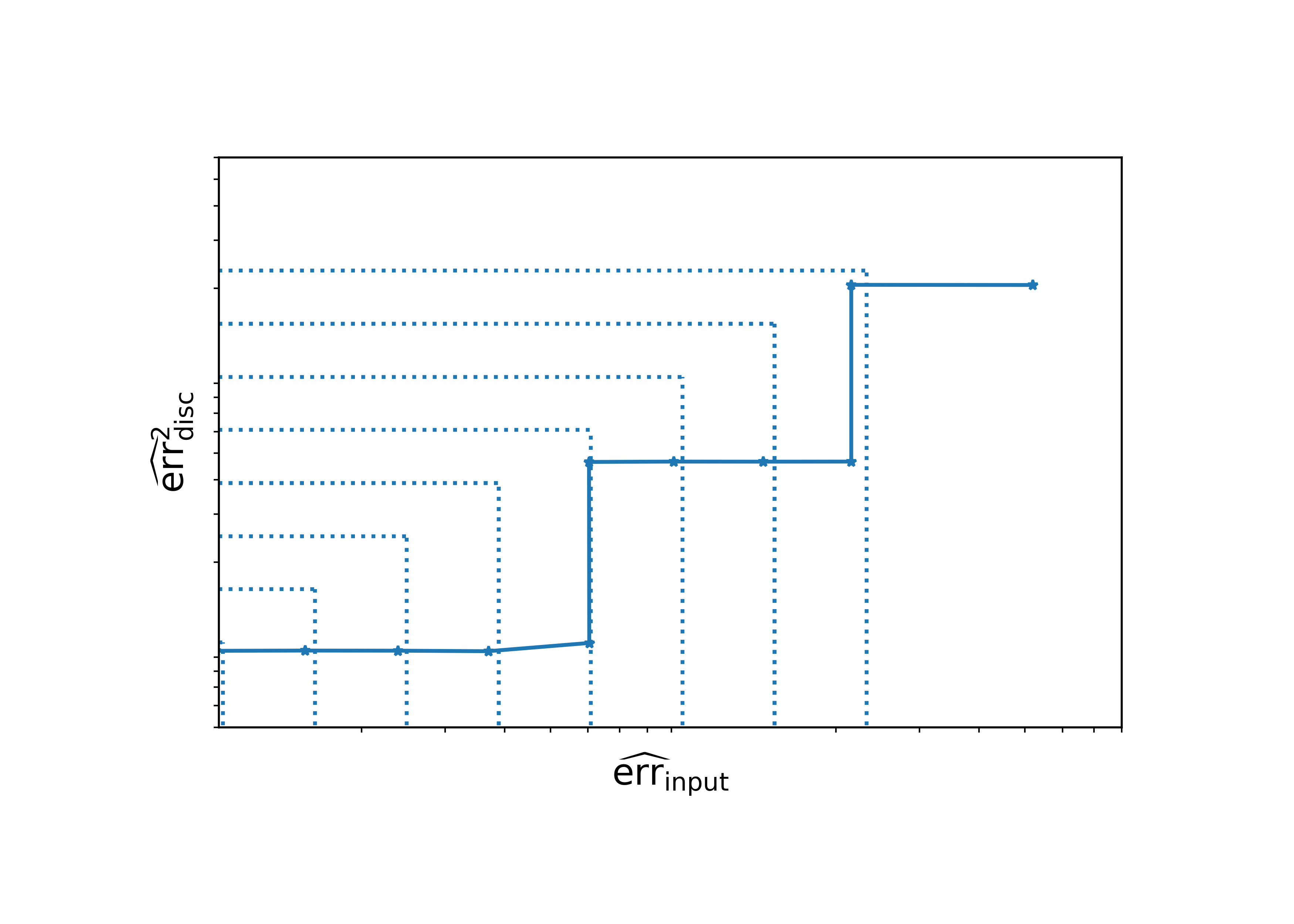
Figure 1: Illustration of an example execution of Algorithm 1. The data point in the upper right corner represents the first estimate of $\widehat{\mathrm{err}}_{\mathrm{disc}}^{2}$ and $\widehat{\mathrm{err}}_{\mathrm{input}}$ based on the initial sequence $\{M_{0,\ell}^{\mathrm{init}}\}_{\ell=0}^{L_{0}}$. The doted squares represent the target MSEs $\epsilon_{\texttt{i}}^{2}$ in each estimation round and illustrate the overlapping subproblems. Hence, Algorithm 1 solves in each estimation round the optimization problem (10) or adapts the highest level $L_{\texttt{i}}$. The joint effort of each estimation round finally solves 2.5.

Remark 2.6.

The actual implementation in C++ [59] is not done with a recursive function but in an equivalent formulation with a while-loop. This is also often called a bottom up implementation which has the advantage over the recursive implementation (top down) to avoid an increased memory consumption on the stack. However, the recursive formulation is easier to derive mathematically. We further remark the inverted level loop which has benefits for the load distribution [5] as illustrated in Fig. 2.

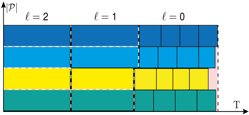
Figure 2: Load balancing of a single exemplary estimation round on three levels with $M_{0}=16$, $M_{1}=2$ and $M_{2}=1$. The sample on level two is processed on all four processes at first. Next, two samples on level one follow where each one is computed on two processes. Lastly sixteen samples on level zero are computed, where each processor handles four individual samples. The light red areas correspond to parallelization losses due to either idling processes (red areas) or due to communication losses (dashed red lines, corresponding to communication across subdomains). The remaining colors repent one of four processing units. The black dashed lines represent transitions between levels, the red dashed lines represent parallelization losses in the FEM system.

Lastly, we present in Algorithm 1 the final BMLMC method as a recursive implementation. For a detailed explanation of the subroutines Welford and MS-FEM, we refer to the upcoming Section 2.5 and to Section 3.

Algorithm 1 Budgeted Multi-Level Monte Carlo

Set the initial sample sequence $\{M_{0,\ell}^{\text{init}}\}_{\ell=0}^{{L_{0}}}$ in $\texttt{data}_{-1}$, a cost budget $\left|\mathcal{P}\right|\cdot\mathrm{T}_{\mathrm{B}}=\mathrm{B}>0$, a splitting parameter $\theta\in(0,1)$ and the reduction factor $\eta\in(0,1)$.

$$\texttt{data}=\left\{\texttt{i}\mapsto\left\{\mathrm{err}_{\texttt{i}},\{M_{\texttt{i},\ell}\}_{\ell=0}^{L_{\texttt{i}}},\{\widehat{\mathrm{Q}}_{\texttt{i},\ell}\}_{\ell=0}^{L_{\texttt{i}}},\{\widehat{\mathrm{C}}_{\texttt{i},\ell}\}_{\ell=0}^{L_{\texttt{i}}},\{\widehat{\mathrm{Y}}_{\texttt{i},\ell}\}_{\ell=0}^{L_{\texttt{i}}},\dots\right\}\right\}$$

$$\texttt{function }\texttt{BMLMC}(\mathrm{B}_{0},\left\{M_{0,\ell}^{\text{init}}\right\}_{\ell=0}^{L_{0}})\colon$$

$$\quad\begin{cases}\texttt{for }\ell={L_{0}},\dots,0\colon&\hskip 8.5359pt{\vartriangle}\texttt{data}_{0,\ell}\leftarrow\texttt{MS-FEM}(M_{0,\ell}^{\text{init}},\mathcal{P})\\ \texttt{data}_{0}\leftarrow\texttt{Welford}(\texttt{data}_{-1},{\vartriangle}\texttt{data}_{0})&\hskip 8.5359pt\texttt{return }\texttt{BMLMC}(\mathrm{B}_{0}-\sum_{\ell=0}^{L_{0}}\mathrm{C}_{\ell},\eta\cdot\mathrm{err}_{0})\end{cases}$$

$$\texttt{function }\texttt{BMLMC}(\mathrm{B}_{\texttt{i}},\epsilon_{\texttt{i}})\colon$$

$$\quad\begin{cases}\texttt{if }\mathrm{B}_{\texttt{i}}\approx 0\colon&\hskip 5.69046pt\texttt{return }\mathrm{err}_{\texttt{i}-1}\\ \texttt{if }\widehat{\mathrm{err}}_{\texttt{disc}}(\texttt{data}_{\texttt{i}-1})\geq\sqrt{1-\theta}\epsilon_{\texttt{i}}\colon&\hskip 5.69046pt{L_{\texttt{i}}}\leftarrow{L_{\texttt{i}}}+1\\ \texttt{if }\widehat{\mathrm{err}}_{\texttt{input}}(\texttt{data}_{\texttt{i}-1})\geq\theta\epsilon_{\texttt{i}}^{2}\colon&\hskip 5.69046pt\widehat{M}_{\texttt{i},\ell}^{\text{opt}}\leftarrow~{}\eqref{eq:optimal-Ml-estimated}\\ \texttt{for }\ell={L_{\texttt{i}}},\dots,0\colon&\hskip 5.69046pt{\vartriangle}M_{\texttt{i},\ell}\leftarrow\max\left\{\widehat{M}_{\texttt{i},\ell}^{\text{opt}}-M_{\texttt{i}-1,\ell},\,0\right\}\\ \widehat{\mathrm{C}}_{\texttt{i}}\leftarrow\sum_{\ell=0}^{L_{\texttt{i}}}{\vartriangle}M_{\texttt{i},\ell}\widehat{\mathrm{C}}_{\texttt{i}-1,\ell}\\ \texttt{if }\widehat{\mathrm{C}}_{\texttt{i}}=0\colon&\hskip 5.69046pt\texttt{return }\texttt{BMLMC}(\mathrm{B}_{\texttt{i}},\eta\cdot\epsilon_{\texttt{i}})\\ \texttt{if }\widehat{\mathrm{C}}_{\texttt{i}}>\mathrm{B}_{\texttt{i}}\colon&\hskip 5.69046pt\texttt{return }\texttt{BMLMC}(\mathrm{B}_{\texttt{i}},0.5\cdot(\epsilon_{\texttt{i}}+\epsilon_{\texttt{i}-1}))\\ \texttt{for }\ell={L_{\texttt{i}}},\dots,0\colon&\hskip 5.69046pt{\vartriangle}\texttt{data}_{\texttt{i},\ell}\leftarrow\texttt{MS-FEM}({\vartriangle}M_{\texttt{i},\ell},\mathcal{P})\\ \texttt{data}_{\texttt{i}}\leftarrow\texttt{Welford}(\texttt{data}_{\texttt{i}-1},{\vartriangle}\texttt{data}_{\texttt{i}})&\hskip 5.69046pt\texttt{return }\texttt{BMLMC}(\mathrm{B}_{\texttt{i}}-\sum_{\ell=0}^{L_{\texttt{i}}}\mathrm{C}_{\ell},\epsilon_{\texttt{i}})\end{cases}$$

Remark 2.7.

By considering 2.5, we chose to discretize first and optimize then. The downside of this approach is that if $s_{\mathrm{Y}_{\ell}}^{2}$, $\widehat{\mathrm{C}}_{\ell}$, $\widehat{\mathrm{Y}}_{\ell}$ and $\widehat{\alpha}$ are inaccurate, the optimization delivers poor results, too. However, by using dynamic programming we actually discretize, optimize, discretize, optimize, … until the budget is exhausted. Hence, the risk of optimizing for the wrong objective based on inaccurate data is reduced as the simulation runs.

2.5 Parallelization Techniques

Algorithm 1 is designed as a state machine. However, due to the significant computational load involved in solving 2.5, it becomes necessary to distribute the workload across multiple nodes or processing units. As a result, Algorithm 1 needs to be transformed into a distributed state machine, i.e., a computational method on interconnected nodes or processing units that synchronizes and maintains a shared state. In this context, the shared state refers to the data containing the estimated errors and sample statistics in the very first line of the algorithm, while the set of processing units $\mathcal{P}$ is responsible for dividing the work and minimizing $\widehat{\mathrm{err}}_{\text{MSE}}$.

Algorithm 2 Welford’s Online Update Method

Compute for $\big{\{}\{\texttt{data}_{\texttt{i},\ell}\}_{\ell=0}^{L_{\texttt{i}}}\big{\}}_{\texttt{i}=A,B}=\big{\{}\{M_{\texttt{i},\ell},\widehat{\mathrm{Q}}_{\texttt{i},\ell},S_{\mathrm{Q}_{2,\texttt{i},\ell}},\dots\}_{\ell=0}^{L_{\texttt{i}}}\big{\}}_{\texttt{i}=A,B}$

$$\texttt{function Welford}(\texttt{data}_{A},\texttt{data}_{B}))\colon$$

$$\begin{cases}M_{AB,\ell}&\quad\leftarrow\quad M_{B,\ell}+M_{A,\ell}\\ \delta_{AB,\ell}&\quad\leftarrow\quad\widehat{\mathrm{Q}}_{B,\ell}-\widehat{\mathrm{Q}}_{A,\ell}\\ \widehat{\mathrm{Q}}_{AB,\ell}&\quad\leftarrow\quad\widehat{\mathrm{Q}}_{A,\ell}+\tfrac{M_{B,\ell}}{M_{AB,\ell}}\delta_{AB,\ell}\\ S_{\mathrm{Q}_{2,AB,\ell}}&\quad\leftarrow\quad S_{\mathrm{Q}_{2,A,\ell}}+S_{\mathrm{Q}_{2,B,\ell}}+\tfrac{M_{A,\ell}M_{B,\ell}}{M_{AB,\ell}}\delta_{AB,\ell}^{2}\\ s_{\mathrm{Q}_{AB,\ell}}^{2}&\quad\leftarrow\quad(M_{AB,\ell}-1)^{-1}S_{\mathrm{Q}_{2,AB,\ell}}\\[2.84526pt] \texttt{return }&\{M_{AB,\ell},\widehat{\mathrm{Q}}_{AB,\ell},\,S_{\mathrm{Q}_{2,AB,\ell}},\dots\}_{\ell=0}^{L_{\texttt{i}}}\end{cases}$$

To achieve this, we discuss the functionality of Algorithm 2 representing the subroutine Welford in Algorithm 1. We use concepts introduced by [15, 58], which were further expanded in [48], to stably compute sample statistics in an incremental and parallel manner.

In particular as illustrated in Fig. 3, Algorithm 2 is first used to incrementally update the sample statistics on individual processes, then again to merge the computations recursively across multiple processing units and lastly, Algorithm 2 is utilized one more time to update the statistical quantities over several estimation rounds. This last step is denoted in Algorithm 1, however, the other two updates happen within MS-FEM for which we refer to the upcoming Section 3. Essentially, we combine in MS-FEM a finite element parallelization with a sample distribution. The resulting inherent parallelization of the algorithm can be classified according to the criteria defined in [5, 25] and [10, 22, 33] as a dynamic and heterogeneous sample and solver parallelization in a single program multiple data framework. A detailed discussion is given in [8, Section 3.5.4].

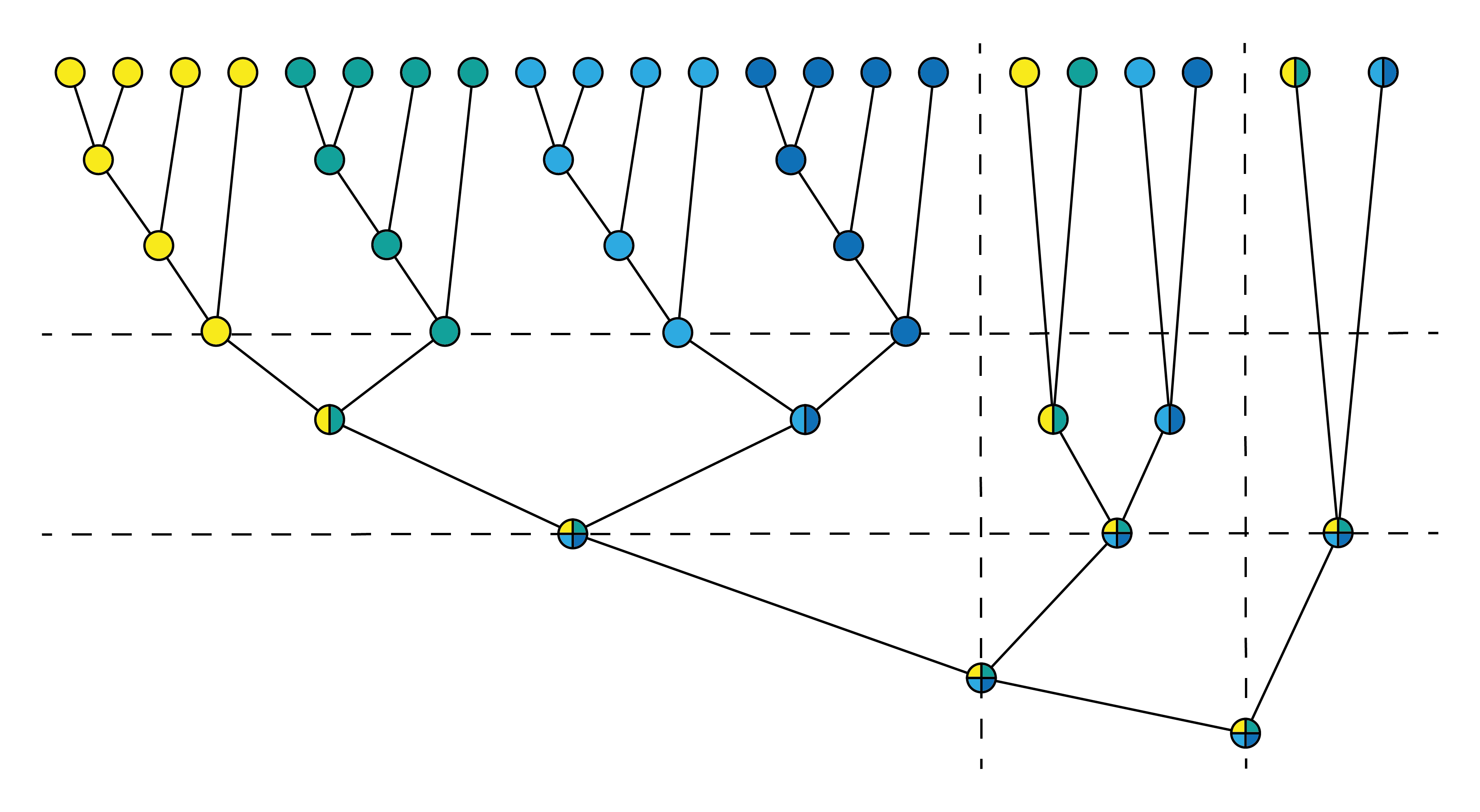
Figure 3: Illustration of the update technique as binary-tree using Algorithm 2 on four parallel processes each represented with another color and over three estimation rounds separated by the vertical dashed lines.

Lastly, we present a proof on Proposition 2.3. The idea is to combine Gustafson’s law [32] with Theorem 2.2. Gustafson’s law describes the theoretical slowdown of an already parallelized task, if it is executed on a serial machine. The motivation behind this law is to describe how more processing units can be utilized to solve larger problems in the same amount of time, i.e., to describe how well the parallelization scales weakly. Translated to the knapsack problem, larger means that we have used more samples and more levels in the final computation. Thereby, we can achieve a smaller estimated RMSE with the same budget in time. Hence, we can measure the weak scaling of the developed parallelization by the development of the estimated error as more processing units are added.

Proof 2.8 (Proof of Proposition 2.3).

The estimates in the edge cases $\lambda_{\mathrm{p}}=1$ of an optimal parallelism $\epsilon\lesssim(\left|\mathcal{P}\right|\cdot\mathrm{T}_{\mathrm{\mathrm{B}}})^{-\delta}=\mathrm{C}_{\epsilon}^{-\delta}$ and $\lambda_{\mathrm{p}}=0$ of a serial execution $\epsilon\lesssim\mathrm{T}_{\mathrm{\mathrm{B}}}^{-\delta}=\mathrm{T}_{\epsilon}^{-\delta}$ simply follow by inversion of Theorem 2.2 for every feasible execution.

To examine $\lambda_{\mathrm{p}}\in(0,1)$, we split the $\epsilon$-time into two parts of the program, a serial part $\lambda_{\mathrm{s}}=1-\lambda_{\mathrm{p}}$ and a parallel part $\lambda_{\mathrm{p}}$ executed on $\left|\mathcal{P}\right|$ processing units, i.e.,

$$\mathrm{T}_{\epsilon,\mathrm{p}}=\lambda_{\mathrm{s}}\mathrm{T}_{\epsilon,\mathrm{p}}+\lambda_{\mathrm{p}}\mathrm{T}_{\epsilon,\mathrm{p}}\,.$$

If the same program is executed on a serial system, the parallelizable part of the system slows down by a factor of $\left|\mathcal{P}\right|^{-\delta}$ to achieve the same RMSE tolerance of $\epsilon$, i.e., the corresponding sequential execution time is

$$\mathrm{T}_{\epsilon,\mathrm{s}}=\lambda_{\mathrm{s}}\mathrm{T}_{\epsilon,\mathrm{p}}+\lambda_{\mathrm{p}}\mathrm{T}_{\epsilon,\mathrm{p}}\left|\mathcal{P}\right|^{-\delta}\,.$$

By this we can deduce the optimal speedup factor of the parallelization

$$\mathrm{S}\coloneqq\frac{\mathrm{T}_{\epsilon,\mathrm{s}}}{\mathrm{T}_{\epsilon,\mathrm{p}}}=\frac{\lambda_{\mathrm{s}}+\lambda_{\mathrm{p}}\left|\mathcal{P}\right|^{-\delta}}{\lambda_{\mathrm{s}}+\lambda_{\mathrm{p}}}=(1-\lambda_{\mathrm{p}})+\lambda_{\mathrm{p}}\left|\mathcal{P}\right|^{-\delta}.$$

Using this speedup factor to determine the additional error reduction by utilizing $\left|\mathcal{P}\right|$ processing units, we get again by the inverted estimate of Theorem 2.2

$$\epsilon \lesssim\mathrm{S}\cdot\mathrm{T}_{\mathrm{\mathrm{B}}}^{-\delta}=\left((1-\lambda_{\mathrm{p}})+\lambda_{\mathrm{p}}\left|\mathcal{P}\right|^{-\delta}\right)\mathrm{T}_{\mathrm{\mathrm{B}}}^{-\delta}.$$

As a consequence, there is a part in the error, denoted with $\epsilon_{\mathrm{s}}$, which can only be reduced with further processing time and another part, denoted with $\epsilon_{\mathrm{p}}$, which can also be mitigated by more processing units

$$\epsilon\lesssim\underbrace{(1-\lambda_{\mathrm{p}})\cdot\mathrm{T}_{\mathrm{\mathrm{B}}}^{-\delta}}_{\eqqcolon\epsilon_{\mathrm{s}}}+\underbrace{\lambda_{\mathrm{p}}\big{(}\left|\mathcal{P}\right|\cdot\mathrm{T}_{\mathrm{\mathrm{B}}}\big{)}^{-\delta}}_{\eqqcolon\epsilon_{\mathrm{p}}}\,.$$

We conclude this section, by summarizing the following limits as a consequence of Proposition 2.3.

	$\lambda_{\mathrm{p}}=0$	$\lambda_{\mathrm{p}}\in(0,1)$	$\lambda_{\mathrm{p}}=1$
$\mathrm{T}_{\mathrm{B}}\rightarrow\infty$	$\epsilon\rightarrow 0$	$\epsilon\rightarrow 0$	$\epsilon\rightarrow 0$
$\left|\mathcal{P}\right|\rightarrow\infty$	$\epsilon\sim 1$	$\epsilon\rightarrow\epsilon_{\mathrm{s}}$	$\epsilon\rightarrow 0$

By this tabel, the BMLMC method is MSE-consistent with respect to the time-budget $\mathrm{T}_{\mathrm{\mathrm{B}}}$ for a fixed set of processing units $\mathcal{P}$. For a fixed time-budget $\mathrm{T}_{\mathrm{\mathrm{B}}}$, the BMLMC method is not MSE-consistent with respect to the amount of processing units $\left|\mathcal{P}\right|$. Hence, there remains a parallelization bias $\epsilon_{\mathrm{s}}$ no matter how manny processing units are added. We refer to Section 5 for numerical experiments on the parallelization and the derived bound.

3 Multi-Sample Finite Element Method

A Finite Element Method (FEM) searches an approximation $\mathbf{u}_{\ell}$ to some PDE in a finite dimensional function space $V_{\ell}$. To construct this space and implement FEMs on a parallel computer, the spatial domain $\mathcal{D}\subset\mathbb{R}^{D}$ is partitioned into subdomains $\mathcal{D}_{P}$ each assigned to a different processing unit $P\in\mathcal{P}$ and decomposed in finitely many cells $K\in\mathcal{K}_{P}$, i.e.,

(21) $$\overline{\mathcal{D}}=\bigcup_{P\in\mathcal{P}}\overline{\mathcal{D}}_{P}=\bigcup_{P\in\mathcal{P}}\bigcup_{K\in\mathcal{K}_{P}}\overline{K}\quad\text{with}\quad K\cap K^{\prime}=\emptyset\quad\text{for}\quad K\neq K^{\prime}\,,$$

where $K\subset\mathcal{D}$ are open sets, $\mathcal{K}=\bigcup_{P\in\mathcal{P}}\mathcal{K}_{P}$ is the collection of all cells on all processing units and $\mathcal{K}_{P}$ is the collection of cells on a single processing unit $P$. The cardinality of the set of processing units $\mathcal{P}$ is assumed to be of power of two to keep the theory aligned with our implementation; however, this is not a necessity and sets of another size might be considered as well. This decomposition of the domain $\mathcal{D}$ further defines a set of vertices $\mathcal{V}$, a set of faces $\mathcal{F}$ and a set of edges $\mathcal{E}$ as explained in the following.

We denote with $\mathcal{F}_{K}$ the set of faces for a cell $K\in\mathcal{K}$ and for all inner faces $F\in\mathcal{F}_{K}\cap\mathcal{D}$, $K_{F}\in\mathcal{K}$ represents the neighboring cell such that $\overline{F}=\partial K\cap\partial K_{F}$. We denote the unit normal vector on the face $F\in\mathcal{F}_{K}$ pointing outwards of $K$ by $\mathbf{n}_{K}$.

Furthermore, $\mathcal{V}_{K}$ denotes the vertices of the cell $K$ and $\mathcal{E}_{F}$ denotes the edges of a face $F\in\mathcal{F}$. Hence, we set $\mathcal{V}=\bigcup_{K\in\mathcal{K}}\mathcal{V}_{K}$, $\mathcal{F}=\bigcup_{K\in\mathcal{K}}\mathcal{F}_{K}$ and $\mathcal{E}=\bigcup_{F\in\mathcal{F}}\mathcal{E}_{F}$ and define a distributed finite element mesh as

$$\mathcal{M}_{\mathcal{P}}\coloneqq\left\{\mathcal{V},\mathcal{K},\mathcal{F},\mathcal{E}\right\}\quad\text{with}\quad\mathcal{M}_{P}\coloneqq\left\{\mathcal{V}_{P},\mathcal{K}_{P},\mathcal{F}_{P},\mathcal{E}_{P}\right\}\,,$$

where $\mathcal{V}_{P}=\bigcup_{K\in\mathcal{K}_{P}}\mathcal{V}_{K}$, $\mathcal{F}_{P}=\bigcup_{K\in\mathcal{K}_{P}}\mathcal{F}_{K}$ and $\mathcal{E}_{P}=\bigcup_{F\in\mathcal{F}_{P}}\mathcal{E}_{F}$ are the vertices, faces and edges on a single processing unit. Note that $\big{\{}\mathcal{V}_{P}\big{\}}$, $\big{\{}\mathcal{F}_{P}\big{\}}$, $\big{\{}\mathcal{E}_{P}\big{\}}$ are overlapping, and $\big{\{}\mathcal{K}_{P}\big{\}}$ is non-overlapping for conforming discretizations; otherwise, the overlap depends on the finite element method.

To construct a mesh hierarchy, the cell diameter $h_{0}$ of a given mesh $\mathcal{M}_{\ell=0,\mathcal{P}}$ is sequentially divided in half $h_{\ell}=h_{0}2^{-\ell}$ with $\ell=0,\dots,L$ as discretization level. This gives the hierarchy

$$\mathcal{M}_{\ell=0,\mathcal{P}}\subset\mathcal{M}_{\ell=1,\mathcal{P}}\subset\dots\subset\mathcal{M}_{\ell=L,\mathcal{P}}\,.$$

More details and several applications of this parallel data structure are given in [9].

3.1 Multi-Mesh Parallelization

To combine the parallelization technique discussed in Section 2.5 with the FE parallelization, we proceed as follows. We distribute the computational units $\mathcal{P}$ across both the set of input samples $\{\mathbf{y}^{(m)}\}_{m=1}^{M_{\ell}}$ and the domain $\mathcal{D}$. Formally, this is expressed as the following resource allocation problem.

Problem 3.1.

Approximate $M_{\ell}$-times a PDE with a FEM on the discretization level $\ell$, such that the communication on a fixed set of processing units $\mathcal{P}$ is minimized.

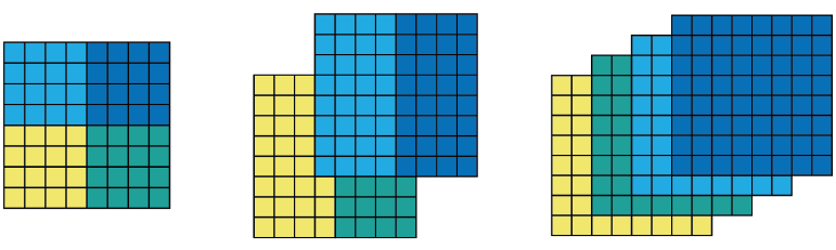
Figure 4: Parallelization approaches for $\mathcal{D}=(0,1)^{2}$ and $\left|\mathcal{P}\right|=4$ according to (22). First, only on spatial domain $\mathcal{D}$ for $M_{\ell}=1$ with $k=2$. Second, mixed parallelization for $M_{\ell}=2$ with $k=1$. Last, only for $M_{\ell}=4$ with $k=0$.

We have to solve this problem within Algorithm 1 whenever the routine MS-FEM is invoked. Considering that we have varying sample sizes across different levels, we find the solution to this problem by examining the following cases.

First, we consider the task to approximate a single $M_{\ell}=1$ sample solution on multiple processing units $\left|\mathcal{P}\right|>1$. Then, the best parallelization is given by the domain decomposition (21) resulting in a single, parallelized mesh $\mathcal{M}_{\mathcal{P}}$ over the domain $\mathcal{D}$. An illustration of this case is given in Fig. 4 on the very left for $\left|\mathcal{P}\right|=4$. Second, if the sample amount equals the amount of processing units $M_{\ell}=\left|\mathcal{P}\right|$, a minimal communication, and thus an optimal parallelization, is achieved by assigning each process its very own unparallelized mesh. This results in the set of meshes $\mathcal{M}_{\mathcal{P}}\coloneqq\{\mathcal{M}^{(m)}_{P}\}_{m=1}^{M_{\ell}}$, i.e., an individual mesh for every single sample as shown in Fig. 4 on the very right.

The more general case, where we compute more samples than available processing units $M_{\ell}>\left|\mathcal{P}\right|$, requires a sequential split of the samples $\sum_{\texttt{j}}{M}_{\texttt{j},\ell}^{\prime}=M_{\ell}$ with ${M}_{\texttt{j},\ell}^{\prime}\leq\left|\mathcal{P}\right|$. Last, we consider the case as depicted in the middle of Fig. 4, where $1<M_{\ell}<\left|\mathcal{P}\right|$. Here, we construct for each $m=1,\dots,M_{\ell}$ a subset of processing units $\mathcal{P}_{k}^{(m)}\in\mathcal{P}$ which can be used to distribute the domain $\mathcal{D}$ on. The subsets $\mathcal{P}_{k}^{(m)}$ are disjoint and of size $|\mathcal{P}_{k}^{(m)}|=2^{k}$ where $k\in\mathbb{N}_{0}$ is chosen such that

(22) $$2^{k}\leq\frac{\left|\mathcal{P}\right|}{M_{\ell}}<2^{k+1}.$$

By following this rule we construct the set of meshes $\mathcal{M}_{\mathcal{P}}\coloneqq\{\mathcal{M}_{\mathcal{P}_{k}}^{(m)}\}_{m=1}^{M_{\ell}}$, such that we minimize the communication in every estimation round.

3.2 Multi-Sample Finite Element Spaces

We consider the task to compute the FE solution $\mathbf{u}_{\ell}(\omega)\in V_{\ell}$ of $\mathcal{L}_{\ell}(\omega,\mathbf{x})\mathbf{u}_{\ell}(\omega,\mathbf{x})=\mathbf{b}_{\ell}(\omega,\mathbf{x})$ for multiple samples at once. In particular, the parallel data structure presented in the previous Section 3.1 is exploited to define a finite element space incorporating the subsets $\mathcal{P}_{k}^{(m)}\subset\mathcal{P}$.

Definition 3.2.

We call the space

$$V_{\ell}(\mathcal{P})=V_{\ell}(\mathcal{P}_{k}^{(1)})\times\dots\times V_{\ell}(\mathcal{P}_{k}^{(M_{\ell})})=\prod_{m=1}^{M_{\ell}}V_{\ell}(\mathcal{P}_{k}^{(m)})$$

a multi-sample finite element space, where

$$V_{\ell}(\mathcal{P}_{k}^{(m)})\coloneqq\left\{\mathbf{v}_{\ell}\in V_{\ell}\colon\,\mathbf{v}_{\ell}|_{K}\in V_{\ell,K},\,\forall K\in\mathcal{K}(\mathcal{P}_{k}^{(m)}),\,\mathcal{P}_{k}^{(m)}\subset\mathcal{P}\right\}$$

is a finite element space for a single sample, defined on the triangulation $\mathcal{K}(\mathcal{P}_{k}^{(m)})$ where the subdomain of processes $\mathcal{P}_{k}^{(m)}\subset\mathcal{P}$ is chosen with the rule (22) and $V_{\ell,K}$ is a generic local finite element space.

With this definition the task of the multi-sample finite element method (MS-FEM) is to find the coefficients

$$\boldsymbol{\mu}=(\boldsymbol{\mu}_{1}^{(1)},\dots,\boldsymbol{\mu}_{N_{\ell}^{h}}^{(1)},\dots,\boldsymbol{\mu}_{1}^{(M_{\ell})},\dots,\boldsymbol{\mu}_{N_{\ell}^{h}}^{(M_{\ell})})^{\top}\in\mathbb{R}^{M_{\ell}\cdot N_{\ell}^{h}}$$

representing the discrete solution

$$(\mathbf{u}_{\ell})_{m=1}^{M_{\ell}}=\left(\sum_{n=1}^{N_{\ell}^{h}}\boldsymbol{\mu}_{n}^{(m)}\boldsymbol{\psi}_{n}^{(m)}\right)_{m=1}^{M_{\ell}}\in V_{\ell}(\mathcal{P})\,,$$

where $\boldsymbol{\psi}_{n}^{(m)}$ are basis functions of the global finite element space of dimension $N_{\ell}^{h}$.

This formulation is inspired by the implementation in [59], where the parallelization over the samples is realized on the coefficient vector of the FEM. This enables the highly adaptive parallelization scheme needed in the BMLMC method. Finally, the complete procedure is summarized in Algorithm 3.

Algorithm 3 Multi-Sample Finite Element Method

$$\texttt{function MS-FEM}(M_{\ell},\mathcal{P},\ell)\colon$$

$$\begin{cases}k\leftarrow\texttt{use }\eqref{eq:comm-split-formula}\texttt{ with }(M_{\ell},\mathcal{P})\\ \texttt{Generate input samples }\left\{\mathbf{y}^{(m)}\right\}_{m=1}^{M_{\ell}}\\ \texttt{Assemble }\mathcal{L}_{\ell}(\mathbf{y}^{(m)},\mathbf{x})\,\mathbf{u}_{\ell}(\mathbf{y}^{(m)},\mathbf{x})=\mathbf{b}_{\ell}(\mathbf{y}^{(m)},\mathbf{x})\texttt{ for }m=1,\dots,M_{\ell}\\ \texttt{Solve }\mathcal{L}_{\ell}(\mathbf{y}^{(m)},\mathbf{x})\,\mathbf{u}_{\ell}(\mathbf{y}^{(m)},\mathbf{x})=\mathbf{b}_{\ell}(\mathbf{y}^{(m)},\mathbf{x})\texttt{ for }m=1,\dots,M_{\ell}\\ \texttt{Update QoI and Cost with \lx@cref{creftype~refnum}{alg:welfords-weighted-online-update}}\end{cases}$$

Remark 3.3.

The above is applicable to arbitrary finite element spaces, e.g. continuous Lagrange elements, enriched Galerkin elements, Raviart-Thomas elements, space-time discontinuous Galerkin (dG) elements or, as in the upcoming section, to dG elements in space. Further details and experiments can be found in [8].

Since the load distribution is a function of $M_{\ell}$ and $\left|\mathcal{P}\right|$ minimizing the communication, the system in Algorithm 3 is assembled, such that it minimizes the coupling, i.e., the system is decoupled for each sample and mildly coupled on the spatial domain. The assembled system has a block structure and is sparse which is inherited from the sparsity of each finite element discretization block.

4 Discretization of the Acoustic Wave Equation

In our numerical examples, we consider the acoustic wave equation with randomly modeled input data in the form of compressible waves propagating through solids.

Problem 4.1.

Let $\mathcal{D}\subset\mathbb{R}^{D}$ be a domain and $[0,T]\subset\mathbb{R}$ a time interval. We search for the randomly distributed velocity field $\mathbf{v}\colon\Omega\times\mathcal{D}\times[0,T]\rightarrow\mathbb{R}^{D}$ and pressure component $p\colon\Omega\times\mathcal{D}\times[0,T]\rightarrow\mathbb{R}$, such that

$$\left\{\begin{array}[]{rcll}\rho(\omega,\mathbf{x})\partial_{t}\mathbf{v}(\omega,\mathbf{x},t)-\nabla p(\omega,\mathbf{x},t)&=&\mathbf{f}(\omega,\mathbf{x},t)&\mathbf{x}\in\mathcal{D},\,\,\,\,\,t\in(0,T]\\ \kappa(\omega,\mathbf{x})^{-1}\partial_{t}p(\omega,\mathbf{x},t)-\operatorname*{div}\left(\mathbf{v}(\omega,\mathbf{x},t)\right)&=&g(\omega,\mathbf{x},t)&\mathbf{x}\in\mathcal{D},\,\,\,\,\,t\in(0,T]\\ \mathbf{v}(\omega,\mathbf{x},t)\cdot\mathbf{n}&=&0&\mathbf{x}\in\partial\mathcal{D},\,\,t\in[0,T]\\ \mathbf{v}(\omega,\mathbf{x},0)&=&\mathbf{v}_{0}(\omega,\mathbf{x})&\mathbf{x}\in\mathcal{D}\\ p(\omega,\mathbf{x},0)&=&p_{0}(\omega,\mathbf{x})&\mathbf{x}\in\mathcal{D}\end{array}\right.$$

with $\mathbf{f}\colon\Omega\times\mathcal{D}\times(0,T]\rightarrow\mathbb{R}^{D}$ and $g\colon\Omega\times\mathcal{D}\times(0,T]\rightarrow\mathbb{R}$ as right-hand sides and the material parameters $\kappa,\rho\colon\Omega\times\mathcal{D}\rightarrow\mathbb{R}$ modeled as random fields. We further allow for randomly distributed initial data in the velocity component $\mathbf{v}_{0}\colon\Omega\times\mathcal{D}\rightarrow\mathbb{R}^{D}$ and the pressure component $p_{0}\colon\Omega\times\mathcal{D}\rightarrow\mathbb{R}$.

The works [40, 44] discuss sufficient conditions for the well-posedness of 4.1 in the case $\mathcal{D}=\mathbb{R}^{D}$.

4.1 Semi-Discretization with Discontinuous Galerkin Methods

We follow [11] and use a discontinuous Galerkin approximation in space based on the formulation of the acoustic wave equation as a first-order system for a fixed $\omega\in\Omega$, $\mathbf{x}\in\mathcal{D}$ and $t\in(0,1]$ given by

(23) $$\mathrm{M}(\omega,\mathbf{x})\partial_{t}\mathbf{u}(\omega,\mathbf{x},t)+\mathrm{A}\mathbf{u}(\omega,\mathbf{x},t)=\mathbf{b}(\omega,\mathbf{x},t)\quad\text{and}\quad\mathbf{u}(\omega,\mathbf{x},0)=\mathbf{u}_{0}(\omega,\mathbf{x})\,.$$

From now on, we omit the explicit notation of the dependency on $\omega$, $\mathbf{x}$ and $t$. The first oder formulation (23) is derived with the operators

$$\mathbf{u}=\begin{pmatrix}\mathbf{v}\\ p\end{pmatrix},\quad\mathrm{M}\mathbf{u}=\begin{pmatrix}\rho\,\mathbf{v}\\ \kappa^{-1}p\end{pmatrix},\quad\mathrm{A}\mathbf{u}=-\begin{pmatrix}\nabla p\\ \operatorname*{div}\mathbf{v}\end{pmatrix}\quad\text{and}\quad\mathbf{b}=\begin{pmatrix}\mathbf{f}\\ g\end{pmatrix}.$$

This system is approximated in space using discontinuous Galerkin (dG) finite elements

$$V_{\ell,\mathbf{p}}^{\mathrm{dG}}=\left\{\mathbf{u}_{\ell}\in\mathrm{L}^{2}(\mathcal{D};\mathbb{R}^{D+1})\colon\mathbf{u}_{\ell}|_{K}\in V_{K,\mathbf{p}}^{\mathrm{dG}},\,\forall K\in\mathcal{K}\right\}\,,$$

where $V_{K,\mathbf{p}}^{\mathrm{dG}}\coloneqq\mathbb{Q}_{\mathbf{p}}(K;\mathbb{R}^{D+1})$ is the tensor product space of local polynomials on a cell $K\in\mathcal{K}$. In the resulting semi-discrete system, we search for $\mathbf{u}_{\ell}\in V_{\ell,\mathbf{p}}^{\mathrm{dG}}$

$$\mathrm{M}_{\ell}\partial_{t}\mathbf{u}_{\ell}+\mathrm{A}_{\ell}\mathbf{u}_{\ell}=\mathbf{b}_{\ell}\quad\text{and}\quad\mathbf{u}_{\ell}(0)=\mathbf{u}_{\ell,0}\,,$$

with cell-wise constant approximations for $\mathrm{M}_{\ell}$ and $\mathrm{L}_{2}$-projections of $\mathbf{b},\mathbf{u}_{0}$ on $\mathbf{b}_{\ell},\mathbf{u}_{\ell,0}\in V_{\ell,\mathbf{p}}^{\mathrm{dG}}$. The differential operator $\mathrm{A}$ is discretized with a full-upwind scheme

$$\left\langle\mathrm{A}_{\ell}\mathbf{u}_{\ell},\boldsymbol{\phi}_{\ell}\right\rangle_{\mathrm{L}^{2}(\mathcal{D})}=\sum_{K\in\mathcal{K}}\left\langle\mathrm{A}_{\ell,K}\mathbf{u}_{\ell},\boldsymbol{\phi}_{\ell,K}\right\rangle_{\mathrm{L}^{2}(K)}\,,$$

with test functions $\boldsymbol{\phi}_{\ell}=(\boldsymbol{\varphi}_{\ell},\psi_{\ell})\in V_{\ell,\mathbf{p}}^{\mathrm{dG}}$. Each local operator is given in case of Neumann boundary conditions by

$$\left\langle\mathrm{A}_{\ell,K}\mathbf{u}_{\ell},\boldsymbol{\phi}_{\ell,K}\right\rangle_{\mathrm{L}^{2}(K)}= -\left\langle\nabla p_{\ell,K},\boldsymbol{\varphi}_{\ell,K}\right\rangle_{\mathrm{L}^{2}(K)}-\left\langle\operatorname*{div}\mathbf{v}_{\ell,K},\psi_{\ell,K}\right\rangle_{\mathrm{L}^{2}(K)}$$

$$-\sum_{F\in\mathcal{F}_{K}\cap\mathcal{D}}\frac{1}{Z_{K}+Z_{K_{F}}}\left\langle\llbracket p_{\ell,K}\rrbracket_{F}+Z_{K_{F}}\llbracket\mathbf{v}_{\ell,K}\rrbracket_{F}\cdot\mathbf{n}_{K},\,\psi_{\ell,K}+Z_{K}\boldsymbol{\varphi}_{\ell,K}\cdot\mathbf{n}_{K}\right\rangle_{\mathrm{L}^{2}(F)}$$

$$+\sum_{F\in\mathcal{F}_{K}\cap\partial\mathcal{D}}Z_{K}\left\langle\mathbf{v}_{\ell,K}\cdot\mathbf{n}_{K},\,\psi_{\ell,K}+Z_{K}\boldsymbol{\varphi}_{\ell,K}\cdot\mathbf{n}_{K}\right\rangle_{\mathrm{L}^{2}(F)}$$

where $Z_{K}=\sqrt{\kappa_{K}\rho_{K}}$ is the impedance and $\llbracket\mathbf{v}_{\ell,K}\rrbracket_{F}=\mathbf{v}_{\ell}|_{K_{F}}-\mathbf{v}_{\ell}|_{K}$ is the jump at inner faces $F\in\mathcal{F}\cap\mathcal{D}$. In [20] it is shown that the system is the well-posed, also for more general boundary conditions.

4.2 Time-Discretization with Implicit Methods

We follow [11, Section 3] and shortly outline the usage of the implicit mid-point rule with the time-step size $\tau_{\ell}=T/N_{\ell}^{\tau}$ and the time-steps $t_{n}=n\tau_{\ell}$, $n=0,\dots,N_{\ell}^{\tau}$, i.e., we construct a sequence of approximations $\mathbf{u}_{\ell}(t_{n})\in V_{\ell,\mathbf{p}}^{\text{dG}}$ with the initial value of $\mathbf{u}_{\ell}(t_{0})=\mathbf{u}_{0}$ by

(24) $$\left(\mathrm{M}_{\ell}+\frac{\tau_{\ell}}{2}\mathrm{A}_{\ell}\right)\mathbf{u}_{\ell}(t_{n})=\left(\mathrm{M}_{\ell}-\frac{\tau_{\ell}}{2}\mathrm{A}_{\ell}\right)\mathbf{u}_{\ell}(t_{n-1})+\tau_{\ell}\mathbf{b}_{\ell}(t_{n-1/2}).$$

By [11, Theorem 3.1] the above system is well-posed and therefore the implicit midpoint rule is applicable. The downside of this implicit method is that the new iteration $\mathbf{u}^{n+1}$ is only implicitly given. Thus, a system of algebraic equations has to be solved in each time-step which can increase the cost of the method significantly.

However, in the context of hyperbolic PDEs the usage of implicit methods avoids stability issues, if the Courant–Friedrichs–Lewy (CFL) condition [21]

(25) $$\frac{\tau_{\ell}}{h_{\ell}}\leq C_{\mathrm{CFL}}\quad\Longleftrightarrow\quad\tau_{\ell}\leq C_{\mathrm{CFL}}\cdot h_{0}2^{-\ell}$$

is not satisfied. For our particular problem, this is critical since the wave speed is a random variable in each cell and thus, the right ratio $\tau_{0}/h_{0}=C_{\mathrm{CFL}}$ is a local condition leading to global stability issues. The usage of implicit methods avoids this problem, nevertheless, finding the right ratio is still important since too large time-steps lead to worse conditioned systems in (24) and too many time-steps simply might be unnecessary to achieve a smaller overall error. However, it is shown in [11, Lemma 3.1] that (24) is well-conditioned and the convergence is independent of the mesh size on level $\ell$. In particular, we solve this system using a GMRES solver with a point block Jacobi preconditioner. We refer to Section 5 for an experimental investigation of this issue.

5 Numerical Experiments for the Acoustic Wave Equation

We consider 4.1 and solve it with the methods introduced in the previous sections. In particular, we commit to the following problem and method configurations which will serve, if not stated otherwise, as the default for the numerical experiments.

 

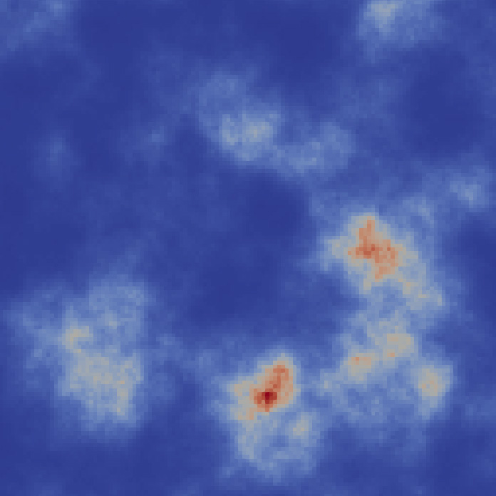
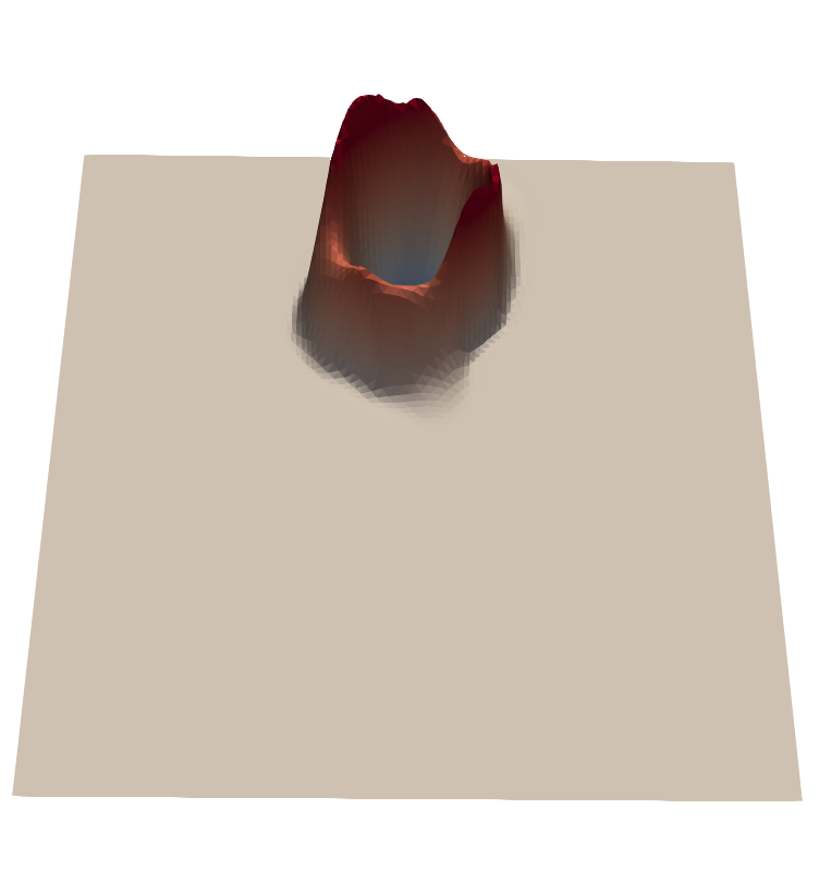
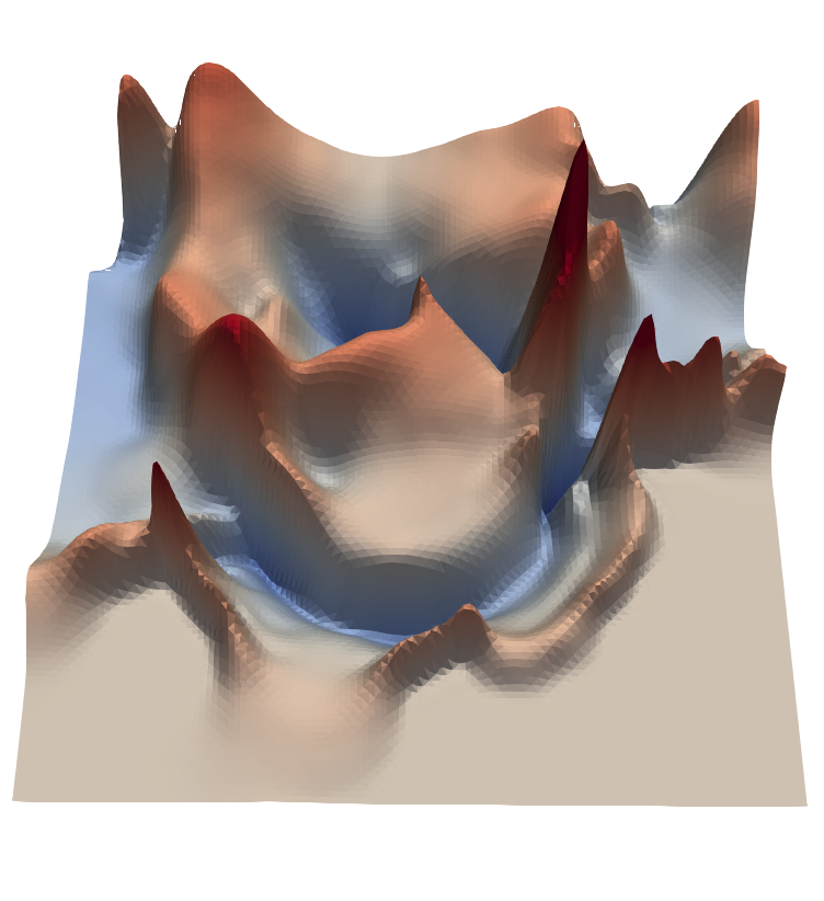
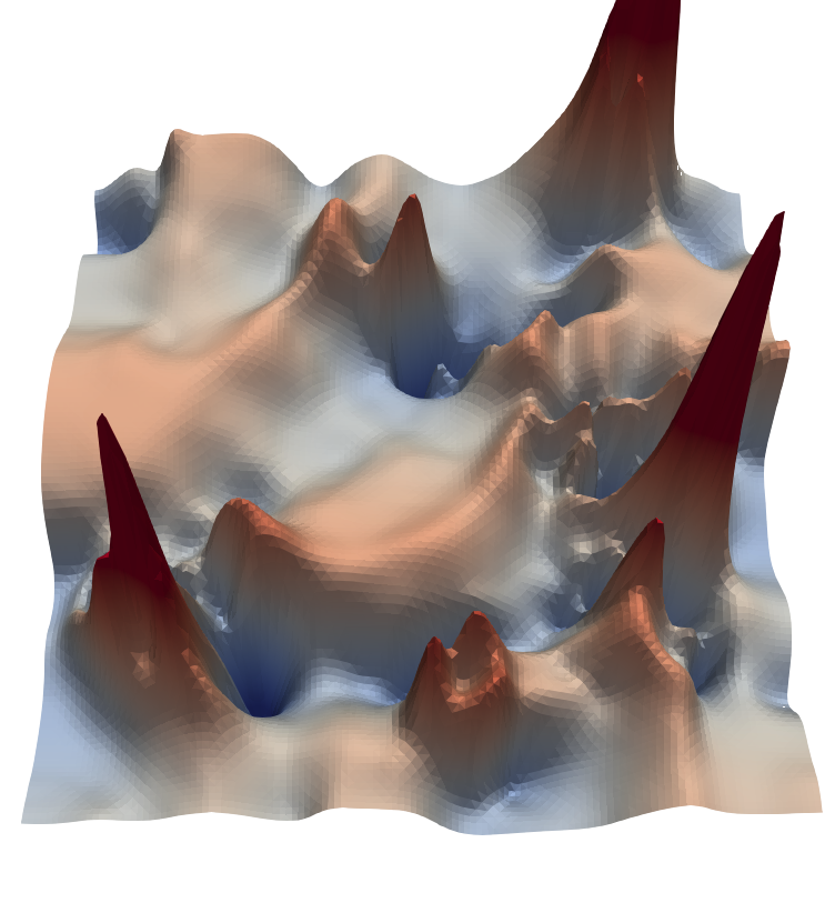
Figure 5: One example realization of the pressure wave approximating 4.1 with log-normal material density $\rho$ (left image) shown at the time points $t=0.0625$, $t=0.5$ and $t=1.0$. The regions of high material density (red areas in left plot) lead to small wave speeds in these regions and thus, to high pressures in the wave.

Problem Configuration

We consider the domain $\mathcal{D}=(0,1)^{2}$, the final time $T=1$ and homogeneous and deterministic initial conditions $(\mathbf{v}_{0},p_{0})=(\mathbf{0},0)^{\top}$.

The right-hand side of 4.1 is deterministically given by $\mathbf{f}\equiv\mathbf{0}$ and $g(\mathbf{x},t)=g_{1}(t)\,g_{2}(\mathbf{x})$, where the function $g_{1}(t)$ is a Ricker wavelet, i.e.,

$$g_{1}(t) =10\left(1-\left(\tfrac{t}{a}\right)^{2}\right)\cdot\exp\left(-\tfrac{t^{2}}{2a^{2}}\right)\quad\text{with}\quad a=\tfrac{\pi}{10},\quad t\in[0,1].$$

The function $g_{2}(\mathbf{x})$ is a nascent delta function centered at $\mathbf{c}=(0.5,0.75)^{\top}$ with an appropriate constant $\overline{g}_{2}$ such that $\left\|g_{2}\right\|_{\mathrm{L}^{1}(\mathcal{D})}=1$ and a diameter $w=0.1$, i.e.,

$$g_{2}(\mathbf{x}) =\begin{cases}\overline{g}_{2}\exp\left(-\left(1-\left\|\frac{\mathbf{x}-\mathbf{c}}{w}\right\|_{2}^{2}\right)^{-1}\right),&\left\|\mathbf{x}-\mathbf{c}\right\|_{2}<w\\ 0,&\left\|\mathbf{x}-\mathbf{c}\right\|_{2}\geq w\end{cases}\qquad\mathbf{x}\in\mathcal{D}.$$

As material, we use a uniformly constant and deterministic compression module $\kappa\equiv 1$ and a log-normally distributed material density $\rho(\omega,\mathbf{x})$, i.e., $\log(\rho(\omega,\mathbf{x}))$ is Gaussian random field with mean-zero and the covariance function

(26) $$\operatorname{Cov}(\mathbf{x}_{1},\mathbf{x}_{2})=\sigma^{2}\exp\left(-\left\|\frac{\mathbf{x}_{1}-\mathbf{x}_{2}}{\lambda}\right\|_{2}^{\nu}\right),$$

where the variance $\sigma=1.0$, the correlation length $\lambda=0.15$ and the smoothing $\nu=1.8$ are used. Defining

$$\rho_{\min}(\omega)\coloneqq\min_{\mathbf{x}\in\mathcal{D}}\rho(\omega,\mathbf{x})\quad\text{and}\quad\rho_{\max}(\omega)\coloneqq\max_{\mathbf{x}\in\mathcal{D}}\rho(\omega,\mathbf{x})$$

gives a distribution of the maximal $c_{\max}(\omega)=\sqrt{\kappa/\rho_{\min}}<\infty$ and the minimal $c_{\min}(\omega)=\sqrt{\kappa/\rho_{\max}}>0$ wave speeds. By [17, Lemma 2.3] realizations are Hölder continuous, and thus $\rho(\omega,\cdot)\in\mathrm{L}^{\infty}(\mathcal{D})$ for a fixed $\omega\in\Omega$. Lastly, we mention that the samples of $\rho$ are generated with the circulant embedding method [23] on the multi-mesh implementation introduced in 3.1. For further details we refer to [8].

The default QoI is the $\mathrm{L}^{2}$-norm for vector valued functions in a region of interest $\mathcal{D}^{\text{RoI}}=(0.25,0.75)\times(0,0.25)$ at time $T=1$, i.e.,

$$\mathrm{Q}(\omega)\coloneqq\left(\int_{0.25}^{0.75}\int_{0}^{0.25}\left|(\mathbf{v},p)^{\top}(\omega,x_{1},x_{2},1)\right|_{2}^{2}\mathrm{d}x_{2}\,\mathrm{d}x_{1}\right)^{1/2},$$

where $\left|\cdot\right|_{2}$ is the Euclidean-norm. The problem configuration is illustrated in Fig. 5 for one particular realization of the input data at the time points $t=0.0625$, $t=0.5$ and $t=1.0$.

Method Configuration

The experiments are conducted on the HoReKa supercomputer for $\mathrm{T}_{\mathrm{B}}=6$ hours using $\left|\mathcal{P}\right|=1024$ processing units. We initialize the BMLMC method on four initial levels starting with the mesh width $h_{0}=2^{-5}$ by

$$\left\{M_{0,\ell}^{\text{init}}\right\}_{\ell=0}^{L_{0}}\coloneqq\left\{M_{0,0}^{\text{init}}=2^{12},\,M_{0,1}^{\text{init}}=2^{10},\,M_{0,2}^{\text{init}}=2^{7},\,M_{0,3}^{\text{init}}=2^{5}\right\}$$

which consumes less than 5% of the total computational budget but already provides good initial estimates. Furthermore, we choose the splitting factor as $\theta=0.5$ and the reduction factor as $\eta=0.9$. The semi-discrete solution is searched in $V_{\ell,\mathbf{p}=2}^{\text{dG}}$ on uniform meshes with $h_{\ell}=h_{0}2^{-\ell}$, which is then solved using an implicit midpoint rule with the time-step size $\tau_{\ell}=2^{-\ell+3}$.

Covariance Function

As start, we examine the influence of the covariance function (26) on the behavior of Algorithm 1. Analytical investigations  [16, 17, 47, 55] as well as experiments [8, 9] for elliptic problems have shown that the structure of the log-normal fields has a large influence on the constant and the convergence rate in Theorem 2.2. We conduct similar investigations for the acoustic wave equation with log-normally distributed material parameters by choosing $\sigma\in\left\{0.5,0.75,1.0\right\}$ in the covariance function (26), while everything else is kept as described in the configurations. The results of this experiment are given in Fig. 6, where in the top row the a posteriori verification of Section 2.1 is given with the estimated exponents $\widehat{\alpha},\widehat{\beta}$ and $\widehat{\gamma}$. In the bottom row, the figure shows the computed amount of samples on each level on the left, the cost distribution over the levels in the middle, and the numerical verification of the convergence of Proposition 2.3 on the right. The x-axis of the lower right plot is the relative left over time budget $(\mathrm{T}_{\mathrm{B},0}-\mathrm{T}_{\mathrm{B},\texttt{i}})/\mathrm{T}_{\mathrm{B},0}$ and the y-axis is the estimated RMSE over the estimation rounds in logarithmic scales. Fig. 6 clearly shows that increasing the variance in (26) worsens the constant in Proposition 2.3, while the measured convergence rate $\widehat{\delta}$, estimated by

$$\min_{(\widehat{\delta},\,\widehat{c}_{\delta})}\sum_{\texttt{i}}\big{(}\log_{2}(\widehat{\mathrm{err}}_{\text{RMSE},\texttt{i}})-\widehat{\delta}\log_{2}((\mathrm{T}_{\mathrm{B},0}-\mathrm{T}_{\mathrm{B},\texttt{i}})/\mathrm{T}_{\mathrm{B},0})+\widehat{c}_{\delta}\big{)}^{2}\,,$$

only changes slightly. We further remark that the BMLMC method works very reliably for this model problem and is capable to exhaust the large computational budget of $\mathrm{B}=1024\cdot 6$ CPU hours feasibly and completely. This can be seen on the middle plot on the bottom, where the total computing times are given by the horizontal lines staying just below the time represented by the red line. Similar investigations for $\nu$ and $\lambda$ in (26) or any sort of input data to 4.1 can be done as well for which we refer again to [8].

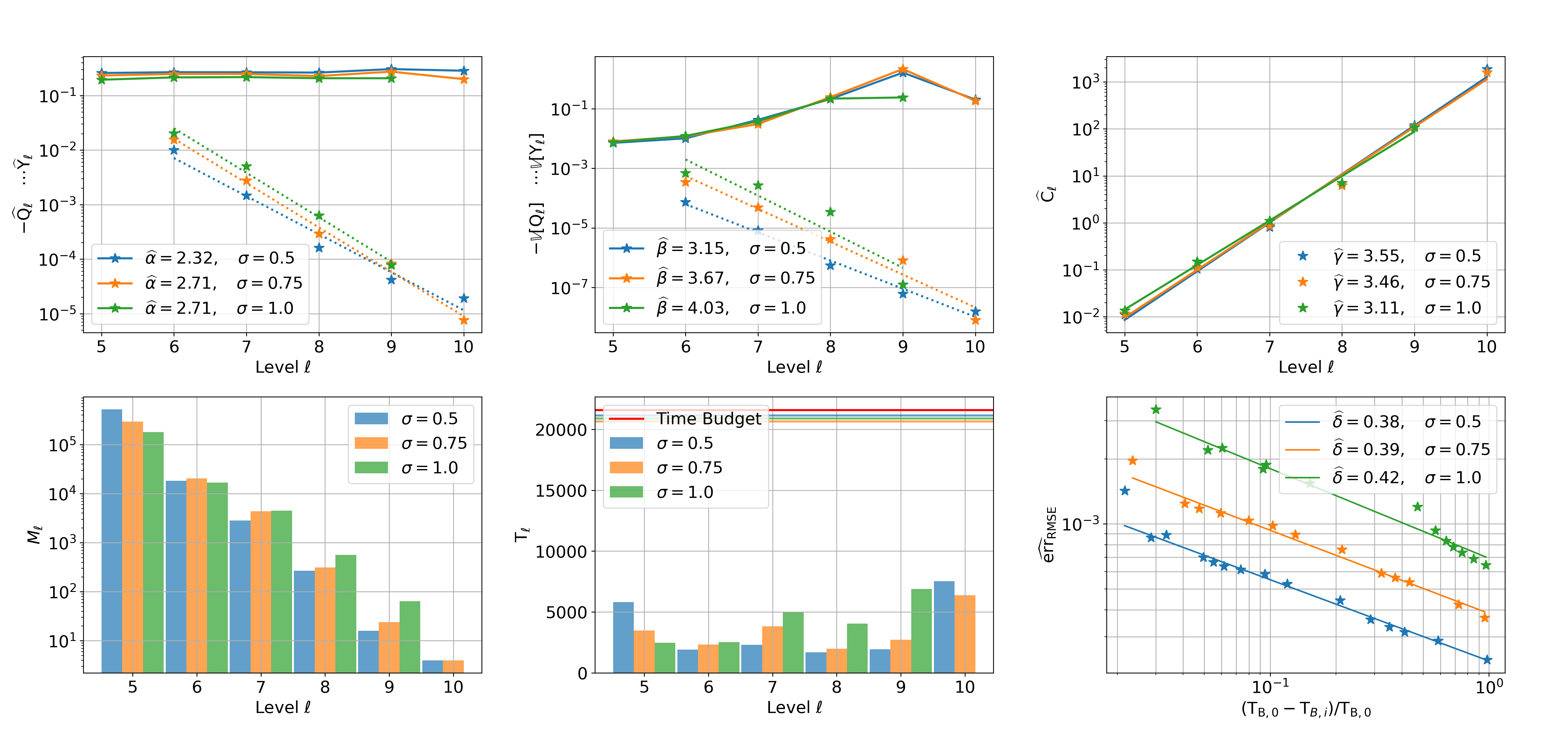
Figure 6: Experiments on the covariance function (26) of the log-normal field.

Time Discretization

We further investigate the time discretization. Even though only shortly discussed in Section 4.2, finding the right time-steps and the right time integrator is crucial for the performance of the overall method and its stability. In Fig. 7, we illustrate the comparison of three different implicit Runge-Kutta methods with the global convergence order of $\mathcal{O}(\tau_{\ell}^{2})$. Particularly, we compare the implicit midpoint rule (IMPR), the Crank Nicolson (CN) method and a third diagonal implicit Runge-Kutta (DIRK) method determined by the Butcher-tableau:

$$\text{DIRK}\colon\,\begin{array}[]{c|cc}1/4&1/4&0\\ 3/4&1/2&1/4\\ \hline\cr&1/2&1/2\end{array}$$

Figure 7: Comparison of different time-stepping methods.

By the lower right plot of Fig. 7, we see that the implicit midpoint rule yields the smallest estimated error and thereby is the best choice out of theses three since we have assigned all three experiments the same computational budget. We suspect that the reason for this is that the evaluations in each time-step in the IMPR are cheaper than for the other two methods. As a consequence of this cost saving, more samples and even one additional level can be computed using the IMPR. We remark that we experimented with explicit Runge-Kutta methods, too, but the time-step sizes $\tau_{\ell}$ had to be drastically reduced in order to stabilize the computation. Locally adaptive schemes as in [31] might overcome this issue, however, we have not been comparing this ansatz to the current implicit approach yet.

We recall the discussion of Section 4.2 and examine the influence of the time-step size on the overall method performance. The results are given in Fig. 8 where we tried out different ratios $\tau_{\ell}/h_{\ell}\in\left\{2^{-1},2^{-2},2^{-3},2^{-4}\right\}$. By the plot on the upper right, we see that the constant $c_{\gamma}$ slightly depends on the time-step as predicted, but also that the variance reduction $\widehat{\beta}$ (upper row in the middle) is heavily influenced. The best choice is $C_{\mathrm{CFL}}=2^{-3}$ again reviled in the lower right plot of Fig. 8. We further remark that with this choice the estimate $\widehat{\gamma}=3.1$ is very close to the best possible value of $\gamma=D+1=3$ as further explained in [36].

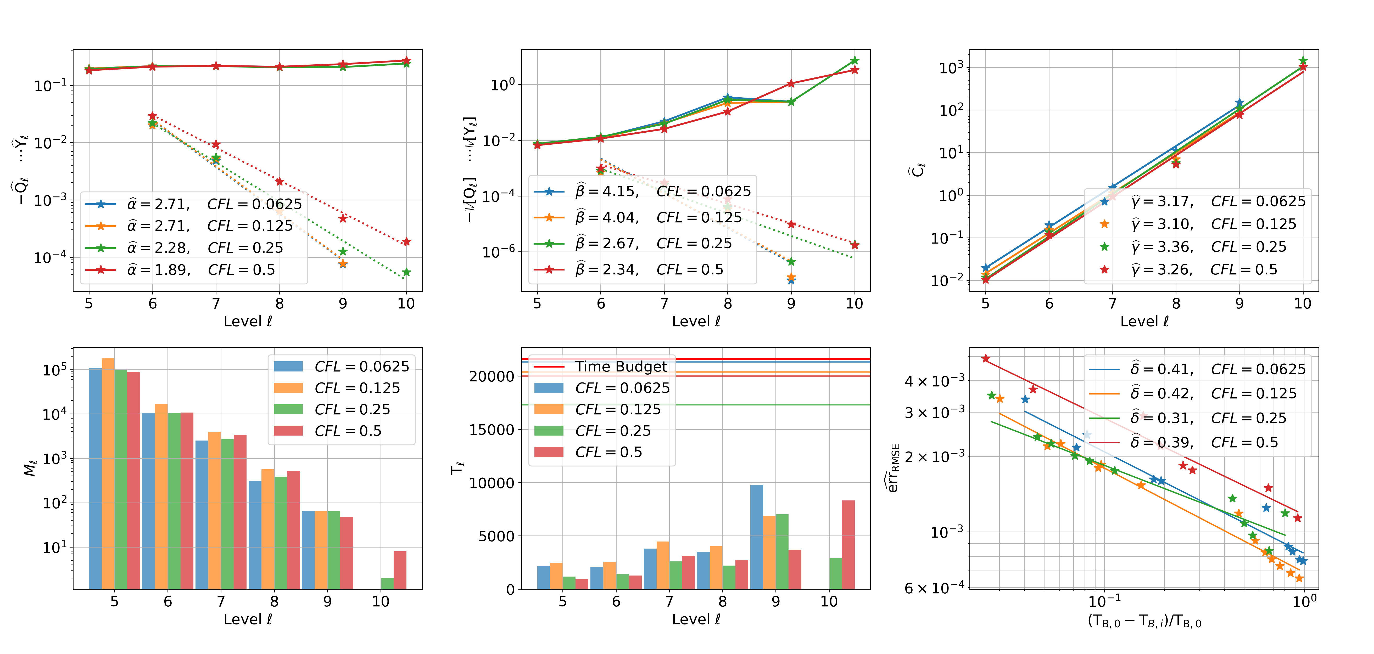
Figure 8: Comparison of different time-step to mesh-width ratios $C_{\mathrm{CFL}}=\tau_{\ell}/h_{\ell}$.

Space Discretization

For the next experiment, we are interested in the polynomial degree of the dG space $V_{\ell,\mathbf{p}}^{\mathrm{d}\mathrm{G}}$. The results in Fig. 9 show that an ansatz space with a higher degree is worth to consider since the $\widehat{\mathrm{err}}_{\mathrm{RMSE}}$ gets smaller with a growing degree even though the cost constant $c_{\gamma}$ (confer upper right plot) is higher. We emphasize that this conclusion is highly problem dependent and that the higher polynomial degree is only worth the additional cost, if the true solution to the PDE provides enough regularity. It is well known, for example given in a discussion in [18], that the cost is dominated by the highest level if $\beta>\gamma$. Contrary to that, if $\beta<\gamma$, the cost is dominated by the lower levels. Both cases can be observed in Fig. 9 on the bar plot in the center of the bottom row, where for $\mathbf{p}=1$ the estimated exponents satisfy $\widehat{\beta}=0.51<3.07=\widehat{\gamma}$ and for $\mathbf{p}=3$ the exponents are given as $\widehat{\beta}=5.44>3.17=\widehat{\gamma}$.

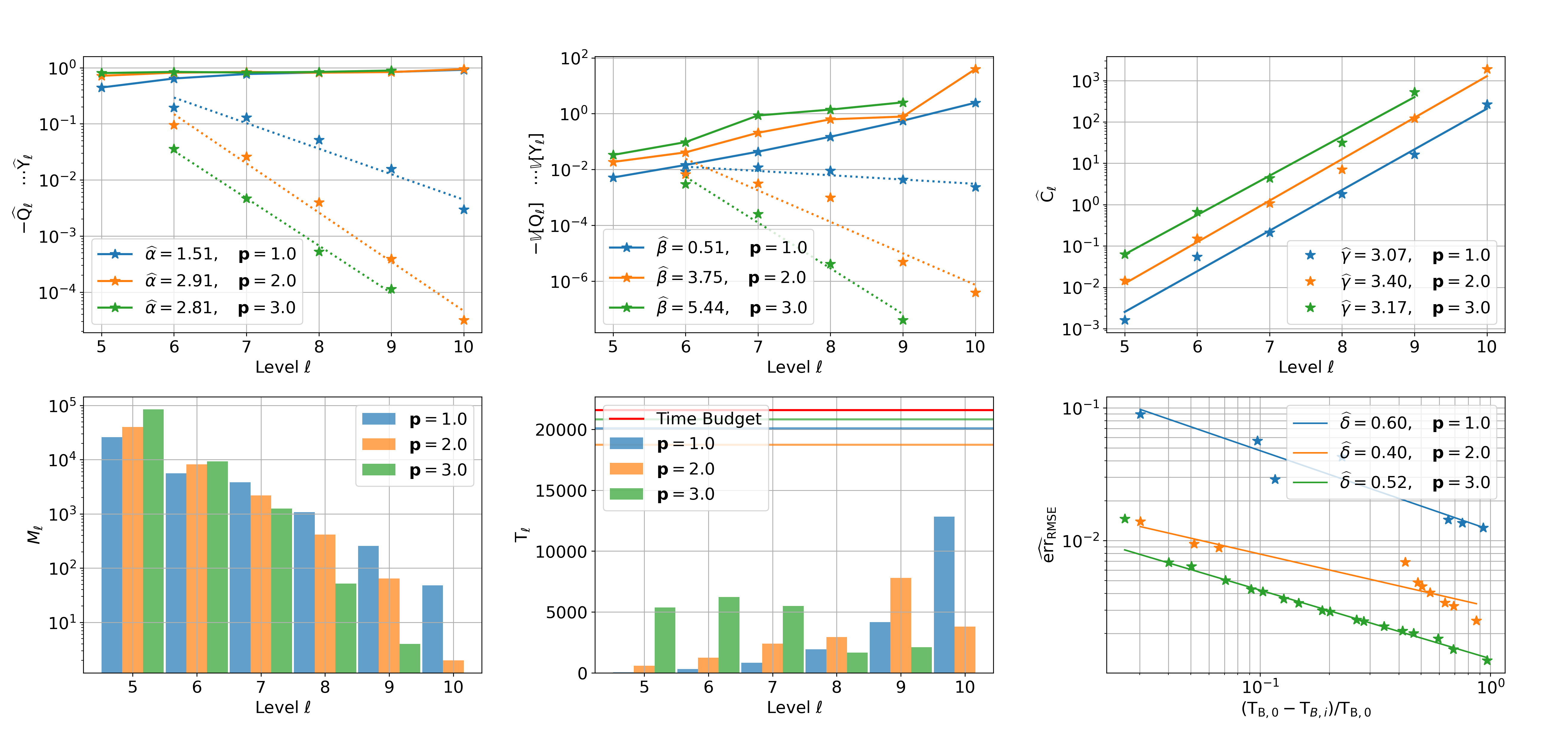
Figure 9: Comparison of different polynomial degrees in the ansatz space $V_{\ell,\mathbf{p}}^{\mathrm{d}\mathrm{G}}$.

Parallelization

Last but not least, we examine the proposed parallelization by conducting a weak scaling experiment, i.e., we increase the computational resources from $\left|\mathcal{P}\right|=128$ to $\left|\mathcal{P}\right|=2048$ and keep the computational time budget fixed at $\mathrm{T}_{\mathrm{B}}=6$ hours. The numerical results of this experiment are summarized in Figure 10. The lower right plot indicates clearly that we effectively reduce the estimated error by utilizing more processing units. However, to examine the influence of the reduction factor $\eta$ and to evaluate the method in the light of Proposition 2.3, we solve the problem again on $\left|\mathcal{P}_{\max}\right|=8192$ and on $\left|\mathcal{P}_{\max}\right|\cdot 2^{-k}$ with $k=1,\dots,7$. Subsequently, we consider the estimated error at the very end of the simulation, i.e. at $(\mathrm{T}_{\mathrm{B},0}-\mathrm{T}_{\mathrm{B},\texttt{i}})/\mathrm{T}_{\mathrm{B},0}=1$ and plot this over $2^{-k}$. With this and (16), we conclude for some $\lambda_{\mathrm{p}}\in(0,1)$

$$\epsilon_{k}\lesssim\epsilon_{\mathrm{s}}+\epsilon_{\mathrm{p},k}=\epsilon_{\mathrm{s}}+\lambda_{\mathrm{p}}(2^{-k}\cdot\left|\mathcal{P}_{\max}\right|\cdot\mathrm{T}_{{\mathrm{B}}})^{-\delta}=\epsilon_{\mathrm{s}}+\lambda_{\mathrm{p}}(\left|\mathcal{P}_{\max}\right|\cdot\mathrm{T}_{{\mathrm{B}}})^{-\delta}\cdot 2^{k\delta}.$$

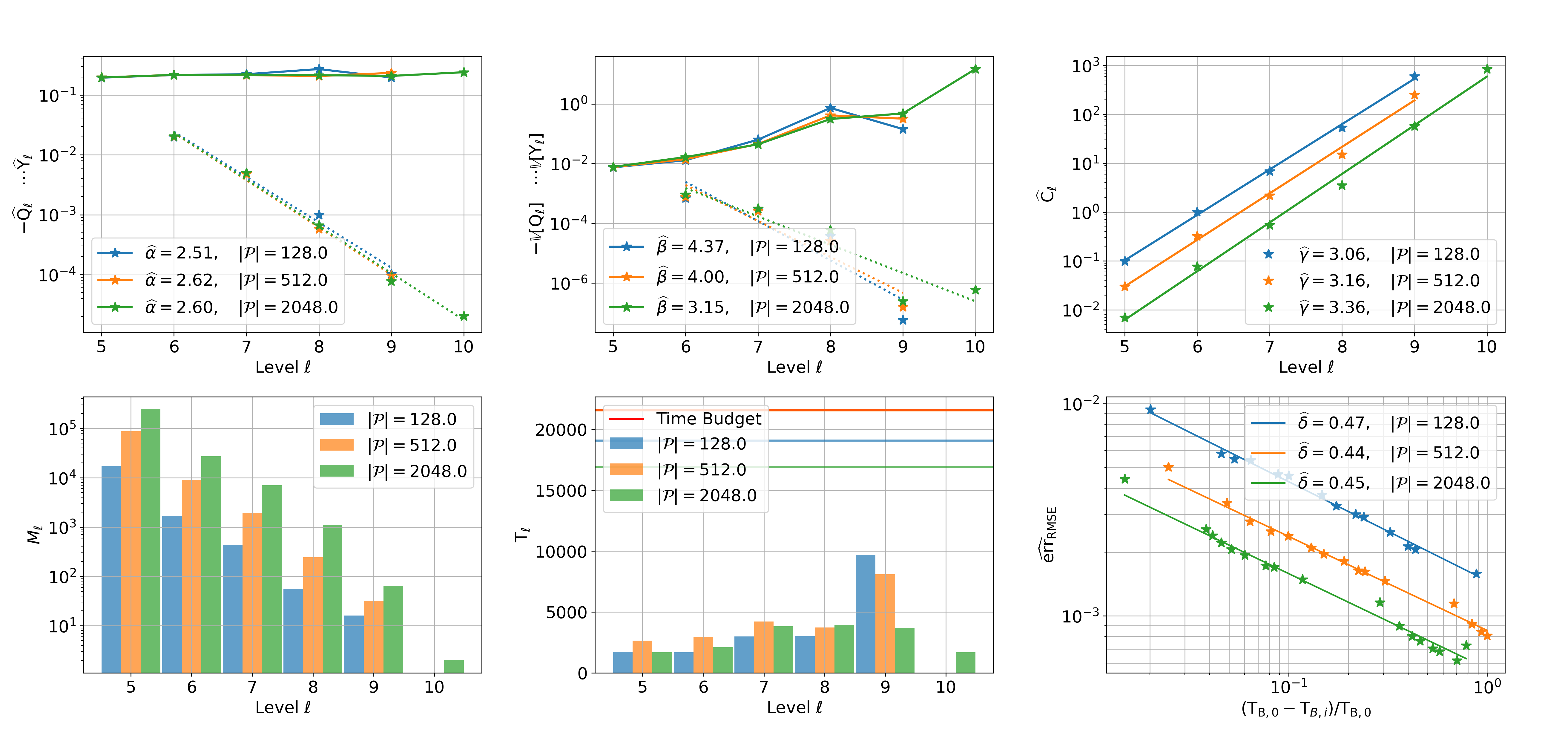
Figure 10: Weak scaling parallelization experiment for a fixed time budget $\mathrm{T}_{\mathrm{B}}$.

This motivates to determine $\widehat{\mathrm{err}}_{\text{RMSE},\mathrm{s}}$ and $\widehat{\mathrm{err}}_{\text{RMSE},\mathrm{p}}$ by fitting the curve

$$\widehat{\mathrm{err}}_{\text{RMSE},k}=\widehat{\mathrm{err}}_{\text{RMSE},\mathrm{s}}+\widehat{\mathrm{err}}_{\text{RMSE},\mathrm{p}}\cdot 2^{k\widehat{\delta}}.$$

The results of these experiments and the fitted curve are given in Figure 11 for $\eta\in\left\{0.7,0.8,0.9\right\}$, which illustrates the influence of the reduction factor on the parallelization. Clearly, we can see in this plot that the smaller the reduction factor, the smaller is the estimated error. This is because the larger reduction factor leads to more frequent synchronizations of the processing units and thus, leading to parallelization losses and ultimately in larger errors. The downside of small reduction factors is the higher probability of exceeding or not fully using the computational budget. In conclusion, in Figure 11 we see that the proposed BMLMC method adheres to the theoretical bound of Proposition 2.3 and that $\lambda_{\mathrm{p}}$ is mostly influenced by the reduction factor $\eta$.

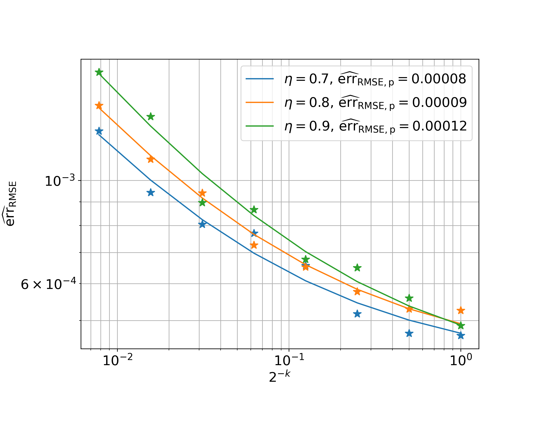
Figure 11: Numerical verification of Proposition 2.3.

6 Discussion, Conclusion and Outlook

We present a novel adaptation of the MLMC method called Budgeted MLMC (BMLMC) method. This approach minimizes the need for prior knowledge, while demonstrating high reliability, robustness, and broad applicability. Furthermore, it achieves exceptional performance within budget constraints and offers full parallelization up to the limits of Gustafson’s law.

The method’s effectiveness stems from three fundamental components: the seamless integration of MLMC with FE methods, the adaptive load distribution within a single distributed data structure according to (22), and the resource allocation within an HPC system following the optimality principle (20).

To demonstrate this experimentally, we conduct investigations on the challenging problem of approximating acoustic wave equations in random and heterogeneous media. Our methodology involves a fully automated process using the continuous delivery pipeline of the software M++ [59] connected to the HoReKa supercomputer. This allows us to reproduce and enhance the numerical results obtained from our implementation.

For a comprehensive explanation of the software, we refer to a forthcoming publication or to [8, 9]. This will provide detailed insights into the software development workflow, as well as highlight the distinguishing features and applications of M++ including space-time discretizations [20, 24], interval arithmetic computations [60], full waveform inversion [11], and other challenging applications like cardio-vascular simulations [26].

This utilization of automated investigations and the empirical search for the optimal algorithm combination provide motivation to view the MLMC method as a knapsack problem. This perspective has facilitated the development of the BMLMC method, incorporating DP techniques and drawing inspiration from the continuation MLMC method [19].

The same approach could potentially be applied to other multi-level UQ algorithms such as multi-level stochastic collocation (MLSC) or multi-level quasi-Monte Carlo (MLQMC) methods. To begin, we recognize that we can utilize the same parallelization strategy and the same distributed data structure. However, DP relies on a nested problem structure. By employing nested sparse grids and suitable lattice rules for QMC, we can preserve this problem structure. This results in a less flexible selection of $\{{\vartriangle}M_{\texttt{i},\ell}\}_{\ell=0}^{L_{\texttt{i}}}$. Furthermore, the on-the-fly estimation of the errors is not as straightforward as it is for simple Monte Carlo methods. Although these methods may be more complex, we anticipate that the benefits of the BMLMC approach can be extended to MLSC and MLQMC methods with careful consideration and adaptation. We leave detailed investigations into these directions open for future work.

Finally, we interpret the consequence of Proposition 2.3. The notion that infinite computing power does not bypass computing time is derived by combining the $\epsilon$-cost theorem and Gustafson’s law. Intuitively, this result makes sense because adding more workers also entails increased synchronization, which prevents the objective from being arbitrarily optimized. Thus, there will always be a synchronization or parallelization bias that can only be mitigated by allocating more time for optimization. The key aspect of demonstrating this insight lies in viewing computing time as a component of the algorithm’s cost and connecting the algorithm’s objective with hardware resources through Gustafson’s law. This idea is quite general, suggesting that similar statements to those in Proposition 2.3 can be derived for other UQ algorithms beyond MLMC, and perhaps even in the realm of machine learning.

References

- [1] The HoreKa (Hochleistungsrechner Karlsruhe) supercomputer at KIT, 2022, https://www.nhr.kit.edu/userdocs/horeka/.
- [2] A. Abdulle, A. Barth, and C. Schwab, Multilevel Monte Carlo methods for stochastic elliptic multiscale PDEs, Multiscale Model. Simul., 11 (2013), pp. 1033–1070, https://doi.org/10.1137/120894725, https://doi.org/10.1137/120894725.
- [3] I. Babuška, F. Nobile, and R. Tempone, A stochastic collocation method for elliptic partial differential equations with random input data, SIAM J. Numer. Anal., 45 (2007), pp. 1005–1034, https://doi.org/10.1137/050645142, https://doi.org/10.1137/050645142.
- [4] I. Babuška, F. Nobile, and R. Tempone, A stochastic collocation method for elliptic partial differential equations with random input data, SIAM Rev., 52 (2010), pp. 317–355, https://doi.org/10.1137/100786356, https://doi.org/10.1137/100786356.
- [5] S. Badia, J. Hampton, and J. Principe, A massively parallel implementation of multilevel Monte Carlo for Finite Element models, arXiv preprint arXiv -2111.11788, (2021).
- [6] M. Ballesio, J. Beck, A. Pandey, L. Parisi, E. von Schwerin, and R. Tempone, Multilevel Monte Carlo acceleration of seismic wave propagation under uncertainty, GEM Int. J. Geomath., 10 (2019), pp. Paper No. 22, 43, https://doi.org/10.1007/s13137-019-0135-5, https://doi.org/10.1007/s13137-019-0135-5.
- [7] A. Barth, C. Schwab, and N. Zollinger, Multilevel Monte Carlo Finite Element Method for elliptic PDEs with stochastic coefficients, Numerische Mathematik, 119 (2011), pp. 123–161.
- [8] N. Baumgarten, A Fully Parallelized and Budgeted Multi-level Monte Carlo Framework for Partial Differential Equations, PhD thesis, Karlsruher Institut für Technologie (KIT), 2023, https://doi.org/10.5445/IR/1000158415.
- [9] N. Baumgarten and C. Wieners, The parallel finite element system M++ with integrated multilevel preconditioning and multilevel Monte Carlo methods, Comput. Math. Appl., 81 (2021), pp. 391–406, https://doi.org/10.1016/j.camwa.2020.03.004, https://doi.org/10.1016/j.camwa.2020.03.004.
- [10] J. Blazewicz, K. Ecker, E. Pesch, G. Schmidt, and J. Weglarz, Handbook on scheduling, Springer, 2019.
- [11] T. Bohlen, M. R. Fernandez, J. Ernesti, C. Rheinbay, A. Rieder, and C. Wieners, Visco-acoustic full waveform inversion: from a DG forward solver to a Newton-CG inverse solver, 2021, https://doi.org/10.1016/j.camwa.2021.09.001, https://doi.org/10.1016/j.camwa.2021.09.001.
- [12] K. M. Bretthauer and B. Shetty, The nonlinear knapsack problem—algorithms and applications, European J. Oper. Res., 138 (2002), pp. 459–472, https://doi.org/10.1016/S0377-2217(01)00179-5, https://doi.org/10.1016/S0377-2217(01)00179-5.
- [13] L. Caccetta and A. Kulanoot, Computational aspects of hard knapsack problems, Nonlinear Anal., 47 (2001), pp. 5547–5558, https://doi.org/10.1016/S0362-546X(01)00658-7, https://doi.org/10.1016/S0362-546X(01)00658-7.
- [14] R. E. Caflisch, Monte Carlo and quasi-Monte Carlo methods, 7 (1998), pp. 1–49, https://doi.org/10.1017/S0962492900002804, https://doi.org/10.1017/S0962492900002804.
- [15] T. F. Chan, G. H. Golub, and R. J. LeVeque, Algorithms for computing the sample variance: analysis and recommendations, Amer. Statist., 37 (1983), pp. 242–247, https://doi.org/10.2307/2683386, https://doi.org/10.2307/2683386.
- [16] J. Charrier, Strong and weak error estimates for elliptic partial differential equations with random coefficients, SIAM J. Numer. Anal., 50 (2012), pp. 216–246, https://doi.org/10.1137/100800531, https://doi.org/10.1137/100800531.
- [17] J. Charrier, R. Scheichl, and A. L. Teckentrup, Finite element error analysis of elliptic PDEs with random coefficients and its application to multilevel Monte Carlo methods, SIAM J. Numer. Anal., 51 (2013), pp. 322–352, https://doi.org/10.1137/110853054, https://doi.org/10.1137/110853054.
- [18] K. A. Cliffe, M. B. Giles, R. Scheichl, and A. L. Teckentrup, Multilevel Monte Carlo methods and applications to elliptic PDEs with random coefficients, Comput. Vis. Sci., 14 (2011), pp. 3–15, https://doi.org/10.1007/s00791-011-0160-x, https://doi.org/10.1007/s00791-011-0160-x.
- [19] N. Collier, A.-L. Haji-Ali, F. Nobile, E. von Schwerin, and R. Tempone, A continuation multilevel Monte Carlo algorithm, BIT, 55 (2015), pp. 399–432, https://doi.org/10.1007/s10543-014-0511-3, https://doi.org/10.1007/s10543-014-0511-3.
- [20] D. Corallo, W. Dörfler, and C. Wieners, Space-time discontinuous Galerkin methods for weak solutions of hyperbolic linear symmetric Friedrichs systems, Tech. Report 1, 2023, https://doi.org/10.1007/s10915-022-02076-3, https://doi.org/10.1007/s10915-022-02076-3.
- [21] R. Courant, K. Friedrichs, and H. Lewy, Über die partiellen Differenzengleichungen der mathematischen Physik, Math. Ann., 100 (1928), pp. 32–74, https://doi.org/10.1007/BF01448839, https://doi.org/10.1007/BF01448839.
- [22] M. A. H. Dempster, J. Kanniainen, J. Keane, and E. Vynckier, High-performance computing in finance: Problems, methods, and solutions, CRC Press, 2018.
- [23] C. R. Dietrich and G. N. Newsam, Fast and exact simulation of stationary Gaussian processes through circulant embedding of the covariance matrix, SIAM J. Sci. Comput., 18 (1997), pp. 1088–1107, https://doi.org/10.1137/S1064827592240555, https://doi.org/10.1137/S1064827592240555.
- [24] W. Dörfler, S. Findeisen, and C. Wieners, Space-time discontinuous Galerkin discretizations for linear first-order hyperbolic evolution systems, Comput. Methods Appl. Math., 16 (2016), pp. 409–428, https://doi.org/10.1515/cmam-2016-0015, https://doi.org/10.1515/cmam-2016-0015.
- [25] D. Drzisga, B. Gmeiner, U. Rüde, R. Scheichl, and B. Wohlmuth, Scheduling massively parallel multigrid for multilevel Monte Carlo methods, SIAM J. Sci. Comput., 39 (2017), pp. S873–S897, https://doi.org/10.1137/16M1083591, https://doi.org/10.1137/16M1083591.
- [26] J. Fröhlich, A segregated finite element method for cardiac elastodynamics in a fully coupled human heart model, PhD thesis, Karlsruher Institut für Technologie (KIT), 2022.
- [27] M. Giles, Improved multilevel Monte Carlo convergence using the Milstein scheme, (2008), pp. 343–358, https://doi.org/10.1007/978-3-540-74496-2_20, https://doi.org/10.1007/978-3-540-74496-2_20.
- [28] M. B. Giles, Multilevel Monte Carlo path simulation, Oper. Res., 56 (2008), pp. 607–617, https://doi.org/10.1287/opre.1070.0496, https://doi.org/10.1287/opre.1070.0496.
- [29] M. B. Giles, Multilevel Monte Carlo methods, Acta Numer., 24 (2015), pp. 259–328, https://doi.org/10.1017/S096249291500001X, https://doi.org/10.1017/S096249291500001X.
- [30] I. G. Graham, F. Y. Kuo, D. Nuyens, R. Scheichl, and I. H. Sloan, Quasi-Monte Carlo methods for elliptic PDEs with random coefficients and applications, J. Comput. Phys., 230 (2011), pp. 3668–3694, https://doi.org/10.1016/j.jcp.2011.01.023, https://doi.org/10.1016/j.jcp.2011.01.023.
- [31] M. J. Grote, S. Michel, and F. Nobile, Uncertainty quantification by multilevel Monte Carlo and local time-stepping for wave propagation, SIAM/ASA J. Uncertain. Quantif., 10 (2022), pp. 1601–1628, https://doi.org/10.1137/21M1429047, https://doi.org/10.1137/21M1429047.
- [32] J. L. Gustafson, Reevaluating amdahl’s law, Communications of the ACM, 31 (1988), pp. 532–533.
- [33] G. Hager and G. Wellein, Introduction to high performance computing for scientists and engineers, CRC Press, 2010.
- [34] A.-L. Haji-Ali, F. Nobile, L. Tamellini, and R. Tempone, Multi-index stochastic collocation for random PDEs, Comput. Methods Appl. Mech. Engrg., 306 (2016), pp. 95–122, https://doi.org/10.1016/j.cma.2016.03.029, https://doi.org/10.1016/j.cma.2016.03.029.
- [35] A.-L. Haji-Ali, F. Nobile, and R. Tempone, Multi-index Monte Carlo: when sparsity meets sampling, Numer. Math., 132 (2016), pp. 767–806, https://doi.org/10.1007/s00211-015-0734-5, https://doi.org/10.1007/s00211-015-0734-5.
- [36] M. Hochbruck, T. Pažur, A. Schulz, E. Thawinan, and C. Wieners, Efficient time integration for discontinuous Galerkin approximations of linear wave equations [Plenary lecture presented at the 83rd Annual GAMM Conference, Darmstadt, 26th–30th March, 2012], ZAMM Z. Angew. Math. Mech., 95 (2015), pp. 237–259, https://doi.org/10.1002/zamm.201300306, https://doi.org/10.1002/zamm.201300306.
- [37] P. Kumar, P. Luo, F. J. Gaspar, and C. W. Oosterlee, A multigrid multilevel Monte Carlo method for transport in the Darcy-Stokes system, J. Comput. Phys., 371 (2018), pp. 382–408, https://doi.org/10.1016/j.jcp.2018.05.046, https://doi.org/10.1016/j.jcp.2018.05.046.
- [38] F. Y. Kuo, C. Schwab, and I. H. Sloan, Quasi-Monte Carlo finite element methods for a class of elliptic partial differential equations with random coefficients, SIAM J. Numer. Anal., 50 (2012), pp. 3351–3374, https://doi.org/10.1137/110845537, https://doi.org/10.1137/110845537.
- [39] A. Litvinenko, A. C. Yucel, H. Bagci, J. Oppelstrup, E. Michielssen, and R. Tempone, Computation of electromagnetic fields scattered from objects with uncertain shapes using multilevel Monte Carlo method, IEEE Journal on Multiscale and Multiphysics Computational Techniques, 4 (2019), pp. 37–50.
- [40] S. Mishra and C. Schwab, Sparse tensor multi-level Monte Carlo finite volume methods for hyperbolic conservation laws with random initial data, Math. Comp., 81 (2012), pp. 1979–2018, https://doi.org/10.1090/S0025-5718-2012-02574-9, https://doi.org/10.1090/S0025-5718-2012-02574-9.
- [41] S. Mishra, C. Schwab, and J. Šukys, Multi-level Monte Carlo finite volume methods for nonlinear systems of conservation laws in multi-dimensions, J. Comput. Phys., 231 (2012), pp. 3365–3388, https://doi.org/10.1016/j.jcp.2012.01.011, https://doi.org/10.1016/j.jcp.2012.01.011.
- [42] S. Mishra, C. Schwab, and J. Šukys, Multilevel Monte Carlo finite volume methods for shallow water equations with uncertain topography in multi-dimensions, SIAM J. Sci. Comput., 34 (2012), pp. B761–B784, https://doi.org/10.1137/110857295, https://doi.org/10.1137/110857295.
- [43] S. Mishra, C. Schwab, and J. Šukys, Multi-level Monte Carlo finite volume methods for uncertainty quantification in nonlinear systems of balance laws, in Uncertainty quantification in computational fluid dynamics, vol. 92 of Lect. Notes Comput. Sci. Eng., Springer, Heidelberg, 2013, pp. 225–294, https://doi.org/10.1007/978-3-319-00885-1_6, https://doi.org/10.1007/978-3-319-00885-1_6.
- [44] S. Mishra, C. Schwab, and J. Šukys, Multi-level Monte Carlo finite volume methods for uncertainty quantification of acoustic wave propagation in random heterogeneous layered medium, J. Comput. Phys., 312 (2016), pp. 192–217, https://doi.org/10.1016/j.jcp.2016.02.014, https://doi.org/10.1016/j.jcp.2016.02.014.
- [45] F. Nobile and R. Tempone, Analysis and implementation issues for the numerical approximation of parabolic equations with random coefficients, Internat. J. Numer. Methods Engrg., 80 (2009), pp. 979–1006, https://doi.org/10.1002/nme.2656, https://doi.org/10.1002/nme.2656.
- [46] F. Nobile, R. Tempone, and C. G. Webster, A sparse grid stochastic collocation method for partial differential equations with random input data, SIAM J. Numer. Anal., 46 (2008), pp. 2309–2345, https://doi.org/10.1137/060663660, https://doi.org/10.1137/060663660.
- [47] F. Nobile and F. Tesei, A Multi Level Monte Carlo method with control variate for elliptic PDEs with log-normal coefficients, Stochastic Partial Differential Equations: Analysis and Computations, 3 (2015), pp. 398–444.
- [48] P. Pébay, T. B. Terriberry, H. Kolla, and J. Bennett, Numerically stable, scalable formulas for parallel and online computation of higher-order multivariate central moments with arbitrary weights, Comput. Statist., 31 (2016), pp. 1305–1325, https://doi.org/10.1007/s00180-015-0637-z, https://doi.org/10.1007/s00180-015-0637-z.
- [49] B. Peherstorfer, K. Willcox, and M. Gunzburger, Survey of multifidelity methods in uncertainty propagation, inference, and optimization, SIAM Rev., 60 (2018), pp. 550–591, https://doi.org/10.1137/16M1082469, https://doi.org/10.1137/16M1082469.
- [50] M. Pisaroni, F. Nobile, and P. Leyland, A continuation multi level Monte Carlo (C-MLMC) method for uncertainty quantification in compressible inviscid aerodynamics, Comput. Methods Appl. Mech. Engrg., 326 (2017), pp. 20–50, https://doi.org/10.1016/j.cma.2017.07.030, https://doi.org/10.1016/j.cma.2017.07.030.
- [51] C.-h. Rhee and P. W. Glynn, Unbiased estimation with square root convergence for sde models, Operations Research, 63 (2015), pp. 1026–1043.
- [52] I. H. Sloan and H. Woźniakowski, When are quasi-Monte Carlo algorithms efficient for high-dimensional integrals?, J. Complexity, 14 (1998), pp. 1–33, https://doi.org/10.1006/jcom.1997.0463, https://doi.org/10.1006/jcom.1997.0463.
- [53] J. Šukys, S. Mishra, and C. Schwab, Static load balancing for multi-level Monte Carlo finite volume solvers, in International Conference on Parallel Processing and Applied Mathematics, Springer, 2011, pp. 245–254.
- [54] A. L. Teckentrup, P. Jantsch, C. G. Webster, and M. Gunzburger, A multilevel stochastic collocation method for partial differential equations with random input data, SIAM/ASA J. Uncertain. Quantif., 3 (2015), pp. 1046–1074, https://doi.org/10.1137/140969002, https://doi.org/10.1137/140969002.
- [55] A. L. Teckentrup, R. Scheichl, M. B. Giles, and E. Ullmann, Further analysis of multilevel Monte Carlo methods for elliptic PDEs with random coefficients, Numer. Math., 125 (2013), pp. 569–600, https://doi.org/10.1007/s00211-013-0546-4, https://doi.org/10.1007/s00211-013-0546-4.
- [56] J. Šukys, Adaptive load balancing for massively parallel multi-level Monte Carlo solvers, in Parallel processing and applied mathematics. Part I, vol. 8384 of Lecture Notes in Comput. Sci., Springer, Heidelberg, 2014, pp. 47–56, https://doi.org/10.1007/978-3-642-55224-3_5, https://doi.org/10.1007/978-3-642-55224-3_5.
- [57] J. Šukys, S. Mishra, and C. Schwab, Multi-level Monte Carlo finite difference and finite volume methods for stochastic linear hyperbolic systems, in Monte Carlo and quasi-Monte Carlo methods 2012, vol. 65 of Springer Proc. Math. Stat., Springer, Heidelberg, 2013, pp. 649–666, https://doi.org/10.1007/978-3-642-41095-6_34, https://doi.org/10.1007/978-3-642-41095-6_34.
- [58] B. P. Welford, Note on a method for calculating corrected sums of squares and products, Technometrics, 4 (1962), pp. 419–420, https://doi.org/10.2307/1266577, https://doi.org/10.2307/1266577.
- [59] C. Wieners, D. Corallo, D. Schneiderhan, L. Stengel, L. Lindner, C. Rheinbay, and N. Baumgarten, Mpp 3.1.5, 2023, https://doi.org/10.35097/1103.
- [60] J. M. Wunderlich, Computer-assisted Existence Proofs for Navier-Stokes Equations on an Unbounded Strip with Obstacle, PhD thesis, Karlsruher Institut für Technologie (KIT), 2022, https://doi.org/10.5445/IR/1000150609.