LBL: Logarithmic Barrier Loss Function for One-class Classification

Abstract

One-class classification (OCC) aims to train a classifier only with the target class data and attracts great attention for its strong applicability in real-world application. Despite a lot of advances have been made in OCC, it still lacks the effective OCC loss functions for deep learning. In this paper, a novel logarithmic barrier function based OCC loss (LBL) that assigns large gradients to the margin samples and thus derives more compact hypersphere, is first proposed by approximating the OCC objective smoothly. But the optimization of LBL may be instability especially when samples lie on the boundary leading to the infinity loss. To address this issue, then, a unilateral relaxation Sigmoid function is introduced into LBL and a novel OCC loss named LBLSig is proposed. The LBLSig can be seen as the fusion of the mean square error (MSE) and the cross entropy (CE) and the optimization of LBLSig is smoother owing to the unilateral relaxation Sigmoid function. The effectiveness of the proposed LBL and LBLSig is experimentally demonstrated in comparisons with several state-of-the-art OCC algorithms on different network structures. The source code can be found at https://github.com/ML-HDU/LBL_LBLSig.

I Introduction

One-class classification (OCC), also known as the anomaly detection (AD), aims to construct the model only exploiting the characteristics of the target data. It has attracted much attention in various communities such as data mining, machine learning and computer vision [1] due to its significance in many applications including cyber-security, financial technology, healthcare, public security and AI safety. The classical methods, such as the one-class support vector machine (OCSVM) [2] and the support vector data description (SVDD) [3], are confronted with difficulties when dealing with high-dimensional and complex data, and such shallow methods are always required feature engineering. In comparisons, the deep learning [4] achieves exceptional successes in addressing high-dimensional and complex data. The promising performance is obtained in the deep learning based OCC algorithms, including the autoencoder (AE) based methods [5, 6, 7, 8, 9, 10, 11, 12, 13, 14, 15, 16, 17], the generative adversarial network (GAN) based methods [18, 19, 20, 21, 22, 23, 24], and other discrimination-based methods [25, 26, 27, 28, 29, 30, 31].

However, little attention is paid to the OCC loss function design. The recent OCC loss functions are developed in [27] and [28]. Ruff et al. [27] proposes the soft-boundary loss (SBL) that can be regarded as the extension in OCC of the mean square error (MSE). But the SBL is only demonstrated on the LeNet-type convolution neural network (CNN) and the performance is not promising. It can be seen from the subsequent sections that the SBL is essentially the hard sample mining with hinge function form and thus it is non-smooth and difficult to optimize [32]. Different from the MSE-type SBL, a cross entropy (CE)-type loss function named HRN that consists of a negative log-likelihood (NLL) term and the gradient penalty term with respect to inputs is proposed in [28]. The HRN shows the surprising results but the performance both in theory and experiment is only verified on the simple multilayer perceptron (MLP). Particularly, we find that the HRN is optimized difficultly in practice and the performance is poor on the CNN. Therefore, it still lacks effective OCC loss functions for deep learning.

Actually, OCC aims to seek a hypersphere with the minimum radius to enclose the target data. In this paper, a novel logarithmic barrier function [33] based OCC loss function (LBL) is first proposed by approximating the OCC objective smoothly. The LBL assigns larger gradients to these samples close to boundary, and thus achieves more compact hypersphere. However, the direct approximation by the logarithmic barrier function may cause the instability especially when samples lie on the boundary leading to the infinity loss. To address this issue, then, a unilateral relaxation Sigmoid function is introduced into LBL and a novel OCC loss named LBLSig is proposed. Owing to the unilateral relaxation Sigmoid function, the optimization becomes smoother. Particularly, LBLSig can be seen as the fusion of MSE and CE. To demonstrate the performance of the proposed OCC loss functions, comparisons with SBL and HRN on different network structures, including the LeNet-type CNN in [27] (named DSLeNet), the MLP and the OCITN in [29], are conducted. Comparisons with several state-of-the-art (SOTA) deep OCC algorithms are also provided. The experimental results demonstrate the superior performance of our proposed algorithms.

II Related Work

II-A Literature Review

Classical machine learning algorithms, such as the Parzen density estimation, k-nearest neighbor (KNN), principal component analysis (PCA), and so on, have been developed for OCC [34]. Particularly, the OCSVM [2] and SVDD [3] are two classical OCC algorithms. The former aims to find a hyperplane to separate the target data from the origin with the maximum possible margin and the latter finds the smallest hypersphere for data separation.

However, the classical machine learning algorithms are generally less effective in characterizing complex and high dimensional data. Thus, a lot of deep learning based OCC algorithms are developed. Deep autoencoder (AE) are the popular approach for OCC [5, 6, 7, 8, 9, 10, 11, 12, 13, 14, 15, 16, 17]. AE learns the identity mapping that tries to reconstruct the inputs with the least distortion. It is believed that the unity features of the target data can be obtained by AEs and then the inputs can be reconstructed from the unity features, but it fails for anomaly data. Therefore, either the reconstruction errors are directly used for anomaly detection [5, 6, 7, 8, 9, 10, 11] or the encoder outputs are extracted as features for subsequent OCC algorithms [12, 13, 14, 15, 16, 17]. Besides, the GAN is also widely used in OCC [18, 19, 20, 21, 22, 23, 24]. Similarly, [18, 19, 20] shows the reconstruction-based approach that train the GAN to reconstruct the target samples and test a sample using the reconstruction error by latent space optimization. Different from that, OCGAN [23] combines the denoising AE (DAE) with a GAN-style adversarial learning. Specially, OCGAN uses the DAE as the generator to learn the latent distribution that is forced to obey a uniform distribution, and the discriminator is trained to differentiate the real images and fake images generated by the decoder outputs of DAE with the random uniform noises as inputs.

In addition to the above AE-based and GAN-based OCC algorithms, many researches also focus on the deep learning models, the OCC loss function, the learning strategy, and so on [25, 26, 27, 28, 29, 30, 31]. As aforementioned, the MSE- and the CE-type OCC loss functions are proposed in [27] and [28], respectively. Golan et al. [25] constructs a self-labeled dataset using several geometric transformations (GTs) over the original OCC dataset, and then a multiclass classifier is trained over the self-labeled dataset. The experiments show the promising performance of the proposed method but the complexity may be high due to that the 72 GTs are used. The recent researches [30, 31] obtain the SOTA results by using the pretrained networks for feature extraction and then fine-tuning by OCC loss function. Specially, the PANDA in [30] that uses the pretrained ResNet152 as the backbone achieves the SOTA performance. The main contribution is that a regularization term minimizing the difference between the pretrained and fine-tuned network weights is introduced to overcome the catastrophic forgetting in transfer learning (the algorithm is named PANDA-EWC), and meanwhile the diagonal of the Fisher Information matrix is adopted to weight each parameter term. Although the SOTA performance is obtained on CIFAR10 by the pretrained networks based OCC algorithms, it is not a general approach such as in the one-dimensional signal domain. In addition, the ImageNet is a more advanced and bigger dataset than CIFAR10. Therefore, the results is predictable that the pretrained ResNet152 on ImageNet can classify the CIFAR10 with a high accuracy, and even up to 92$\%$ without fine-tuning [30]. It can also be seen from the experiments that we obtain the SOTA performance by simply replacing the OCC loss of original PANDA with the proposed LBL and LBLSig.

II-B Brief review of SBL and HRN

Before introducing the proposed LBL and LBLSig, we briefly review the existing OCC loss functions.

Two OCC loss functions are stated in Ruff et al. [27] including the soft-boundary loss (SBL) and the MSE based OCC loss (MSE-OCL). Given an OCC training set with $N$ samples ${{\bf{x}}_{i}}$, the MSE-OCL seeks a hypersphere centered at $\bf{c}$, that is

$$\min_{\boldsymbol{\mathcal{W}}}\quad\frac{1}{N}\sum_{i=1}^{N}\left\|{{\boldsymbol{\Phi}}\left({\bf{x}}_{i};{\boldsymbol{\mathcal{W}}}\right)-{\bf{c}}}\right\|^{2}+\frac{{\lambda}}{2}\sum_{\ell=1}^{L}\left\|{\bf{W}}^{(\ell)}\right\|_{F}^{2},$$ (1)

where ${\bf{c}}$ is the center of hypersphere, $\lambda$ is the trade-off parameter, and ${\boldsymbol{\Phi}}\left({\bf{x}}_{i};{\boldsymbol{\mathcal{W}}}\right)$ is the model output with the learnable parameter ${\boldsymbol{\mathcal{W}}}=\{{{\bf{W}}^{(1)},\cdots,{\bf{W}}^{(L)}}\}$. It can be readily seen that (1) is a direct extension of MSE based multiclass classification loss (MSE-MCL) that the desired output becomes a constant ${\bf{c}}$ in OCC, and thus the MSE-OCL is similar with the regression. The MSE-OCL is a simple but effective OCC loss function, which can be traced back to [35], and has been widely used in OCC [35, 36, 37, 38, 39, 14, 40, 41]. As aforementioned, the OCC tries to seek the minimum-radius hypersphere centered at ${\bf{c}}$ that encloses the target data. The minimum-radius is obtained implicitly in MSE-OCL by minimizing the distance between the outputs of model ${\boldsymbol{\Phi}}\left({\bf{x}}_{i};{\boldsymbol{\mathcal{W}}}\right)$ and the center $\bf{c}$. Different from that, the SBL which is the main contribution of [27] explicitly minimizes the radius of the hypersphere

$$\min_{R,{\boldsymbol{\mathcal{W}}}} R^{2}+{\frac{{\lambda}_{1}}{N}}\sum_{i=1}^{N}\max\left\{{0,\left\|{{\boldsymbol{\Phi}}\left({\bf{x}}_{i};{\boldsymbol{\mathcal{W}}}\right)-{\bf{c}}}\right\|^{2}-R^{2}}\right\}$$ (2)

$$+\frac{{\lambda}_{2}}{2}\sum_{\ell=1}^{L}\left\|{\bf{W}}^{(\ell)}\right\|_{F}^{2},$$

where $\lambda_{1}$ and $\lambda_{2}$ are the trade-off parameters, $R$ is the radius of hypersphere. It can be readily seen that the SBL explicitly minimizes the hypersphere radius and meanwhile penalizes the target data outputs lying outside the hypersphere, as shown in the second term of (2). However, it is worthy pointing out that the radius in (2) fails to be optimized by the gradient. Combining with the implementation of the SBL, actually, the radius is updated in each mini-batch by choosing a certain quantile from the sequence $\left\|{{\boldsymbol{\Phi}}\left({\bf{x}}_{i};{\boldsymbol{\mathcal{W}}}\right)-{\bf{c}}}\right\|^{2}$, which is also stated in [12]. Therefore, the SBL is the iterative hard sample mining in essence where the radius is determined by ranking the distance from $\bf{c}$ and then it is used to select the hard samples in each mini-batch.

The aforementioned MSE-OCL/SBL is the representative MSE based OCC loss functions in deep learning. Different from that, Hu et al. [28] proposes a novel OCC loss function named HRN that can be seen as an extension of CE in OCC. The HRN consists of the negative log-likelihood (NLL) and the H-Regularization with 2-Norm instance-level normalization [28], that is

$$\small\min_{\boldsymbol{\mathcal{W}}}\quad\underbrace{-\sum_{i=1}^{N}{{\log\left({{\text{Sig}}\left({{\boldsymbol{\Phi}}\left({\bf{x}}_{i};{\boldsymbol{\mathcal{W}}}\right)}\right)}\right)}}}_{\text{NLL}}+{\lambda}\underbrace{\sum_{i=1}^{N}{\left\|{{\nabla}_{\bf{x}}{{\boldsymbol{\Phi}}\left({\bf{x}}_{i};{\boldsymbol{\mathcal{W}}}\right)}}\right\|_{F}^{q}}}_{\text{H-regularization}},$$ (3)

where $\lambda$ is the trade-off parameter, the exponent $q$ is a manual hyperparameter, and $\text{Sig}(\cdot)$ is the Sigmoid function that can be seen as the probability of $\bf{x}$ belonging to the target class. It can be readily seen from NLL term that the model output ${\boldsymbol{\Phi}}({\bf{x}}_{i};{\boldsymbol{\mathcal{W}}})$ is directly fed into the Sigmoid function for probability and minimizing the NLL means to maximize the ${{\boldsymbol{\Phi}}\left({\bf{x}}\right)}$, i.e., train the model to obtain high output value for target data. Actually, the NLL term is essentially the direct extension/degeneration from CE of multiclass classification in which all data are positive samples, i.e., the one-hot label vector in OCC becomes a constant $1$. However, there is no constraint over the growth on the value of ${{\boldsymbol{\Phi}}\left({\bf{x}}\right)}$. When minimizing NLL, the trained weights of the model may have large absolute values to force $\text{Sig}({{\boldsymbol{\Phi}}\left({\bf{x}}\right)})$ to 1. In this way, the anomaly data may also obtain a large output ${{\boldsymbol{\Phi}}\left({\bf{x}}\right)}$ leading to $\text{Sig}({{\boldsymbol{\Phi}}\left({\bf{x}}\right)})=1$. To address this issue, a regularization named H-regularization that can be traced to [42] is developed in [28]. The HRN shows the superior performance than SBL but the method is only conducted and verification on MLP. In practice, we find that the HRN is optimized difficultly and the performance is poor on the CNN.

III The proposed methods

III-A LBL

As aforementioned, OCC aims to seek a hypersphere that encloses the target data. Given a training set with $N$ target samples ${{\bf{x}}_{i}}\in{\mathcal{X}}$, the objective of OCC can be always expressed as

$$Dis\left({{\boldsymbol{\Phi}}({\bf{x}}_{i};{\boldsymbol{\mathcal{W}}}),{\bf{c}}}\right)<R,{\ }i=1,\cdots,N,$$ (4)

where $Dis(\cdot)$ represents a distance function such as the $p$-norm distance $\left\|{\cdot}\right\|_{p}$, the cosine distance, the Chebyshev distance and so on. $R$ is the radius of the hypersphere. Then, a novel loss function is developed by directly approximating the inequality and (4) can be reformulated as [33]

$$\min\limits_{\boldsymbol{\mathcal{W}}}{} \frac{1}{N}\sum\limits_{i=1}^{N}{I\left({u_{i}}\right)+\frac{{\lambda}}{2}\sum_{\ell=1}^{L}\left\|{\bf{W}}^{(\ell)}\right\|_{F}^{2}},$$ (5)

$${\rm{s.}}{\ }{\rm{t.}}{} {u_{i}}={D_{i}^{2}}-R^{2},$$

where $D_{i}={Dis\left({{\boldsymbol{\Phi}}({\bf{x}}_{i};{\boldsymbol{\mathcal{W}}}),{\bf{c}}}\right)}$, $I(u)$ is the indicator function that is defined as

$$I(u)=\left\{\begin{aligned} 0,{\ }&u\leq 0,\\ \infty,{\ }&u>0.\end{aligned}\right.$$ (6)

$I(u)$ tends to infinity when the model output ${\boldsymbol{\Phi}}({\bf{x}}_{i};{\boldsymbol{\mathcal{W}}})$ falls outside the hypersphere $({\bf{c}},{R})$. Thus, minimizing $I(u)$ can enforce ${\boldsymbol{\Phi}}({\bf{x}}_{i};{\boldsymbol{\mathcal{W}}})$ to fall inside the hypersphere $({\bf{c}},{R})$. However, (5) is difficult to be optimized due to that $I(u)$ is not differentiable. To address this issue, the LBL is proposed to approximate (6) smoothly by the logarithmic barrier function $\hat{I}(u)=-\frac{1}{\theta}{\log\left(-{u}\right)}$ [33], that is

$$\min\limits_{\boldsymbol{\mathcal{W}}}{} -\frac{1}{N\theta}\sum\limits_{i=1}^{N}{\log\left(-{u_{i}}\right)+\frac{{\lambda}}{2}\sum_{\ell=1}^{L}\left\|{\bf{W}}^{(\ell)}\right\|_{F}^{2}},$$ (7)

$${\rm{s.}}{\ }{\rm{t.}}{} {u_{i}}={D^{2}_{i}}-R^{2}.$$

Here ${\theta}>0$ controls the approximation precision of the logarithmic barrier function to the indicator function $I(u)$. Figure 1 shows the curves of $\hat{I}(u)$ with different $\theta$. It can be seen that $\hat{I}(u)$ is convex and nondecreasing with respect to $u$. Specially, it increases to $\infty$ smoothly as $u$ increases to $0$ (i.e., ${Dis\left({{\boldsymbol{\Phi}}({\bf{x}}_{i};{\boldsymbol{\mathcal{W}}}),{\bf{c}}}\right)}\geq R$). In addition, the value of $I(u)$ and its gradient with respect to $u<0$ are both equal to $0$ leading to the sample distributions inside the hypersphere unchange. On the contrary, different penalties are assigned to target samples in LBL. Specially, the samples close to the boundary of the hypersphere (i.e., ${Dis\left({{\boldsymbol{\Phi}}({\bf{x}}_{i};{\boldsymbol{\mathcal{W}}}),{\bf{c}}}\right)}\to R$) will obtain higher penalty as well as the larger gradient value, as shown in the figure. In this way, LBL may pay more attention to contract these samples to center ${\bf{c}}$. Those samples away from the boundary that have small loss and gradient value are fine-tuned in the optimization of LBL for better distributions. It should be pointed out that LBL is also affected by the approximation precision $\theta$ but it can be omitted when adding the trade-off parameter $\lambda$ for regularization. Thus, $\theta$ is only set to be $1$ in this paper.

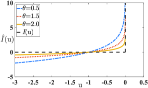
Figure 1: The curves of logarithmic barrier function with different approximate precision $\theta$.

The same observation can be obtained by the gradients. Denote by $J_{1}({\boldsymbol{\mathcal{W}}})=-\frac{1}{N\theta}\sum\limits_{i=1}^{N}{\log\left(-{u_{i}}\right)}$. The gradient of $J_{1}({\boldsymbol{\mathcal{W}}})$ with respect to ${\boldsymbol{\mathcal{W}}}$ can be computed as

$${\frac{\partial{J_{1}}}{\partial{\boldsymbol{\mathcal{W}}}}}={\frac{1}{N\theta}}\sum_{i=1}^{N}{{\frac{1}{-u_{i}}}\cdot{\frac{\partial{D^{2}_{i}}}{\partial{\boldsymbol{\mathcal{W}}}}}}.$$ (8)

It can be seen that the samples close to the boundary of the hypersphere have small $u_{i}$ and thus large gradient values. In this way, the marginal samples can be clustered into $\bf{c}$ effectively. However, the convergence speed is slowed down sharply when ${\boldsymbol{\Phi}}({\bf{x}}_{i};{\boldsymbol{\mathcal{W}}})\to{\bf{c}}$. Hence the fixed and unchanged hypersphere radius $R$ during training may lead to vanishing gradients. To address this issue, the radius $R$ is redetermined manually during training. For example, the $R$ is reset to twice the maximum distance when every several epochs,

$$R=2\cdot\max_{i}{Dis\left({{\boldsymbol{\Phi}}({\bf{x}}_{i};{\boldsymbol{\mathcal{W}}}),{\bf{c}}}\right)}$$ (9)

In this way, LBL is optimized by contracting the hypersphere with radius $R$ and thus keeps a fast learning speed. For the hypersphere center $\bf{c}$, it depends on the models and it will be given in the experiments.

III-B LBLSig

The samples away from the boundary can obtain larger gradients in LBL than those close to center $\bf{c}$. It is similar with the hard sample mining in SBL but LBL is a smooth loss function. However, both the SBL and LBL may suffer from the noises. Specially, the radius $R$ may obtain large value in (9) when mixed with large noises. In this case, the noisy samples always obtain larger gradients and thus the LBL tries to optimize the noisy samples leading to wrong learning. To address this issue, a simple method is to slack the boundary by rejecting a percentage of targets samples, i.e., the radius $R$ is computed by

$$R={{Quantile}}\left({Dis\left({{\boldsymbol{\Phi}}({\bf{x}}_{i};{\boldsymbol{\mathcal{W}}}),{\bf{c}}}\right)},q\right),$$ (10)

where ${Quantile}(\cdot,q)$ computes the $q$-th quantile of the sequence $\{{Dis\left({{\boldsymbol{\Phi}}({\bf{x}}_{i};{\boldsymbol{\mathcal{W}}}),{\bf{c}}}\right)},i=1,\cdots,N\}$. Then, the samples with ${Dis\left({{\boldsymbol{\Phi}}({\bf{x}}_{i};{\boldsymbol{\mathcal{W}}}),{\bf{c}}}\right)}>R$ are discarded. However, the optimization of LBL may be instability especially when samples lie on the boundary leading to the infinity loss and gradient. The above method fails to solve this situation.

Different from the above method, a smooth and robust OCC loss function named LBLSig is further developed in this paper, which can be expressed as

$$\min\limits_{\boldsymbol{\mathcal{W}}}{} -\frac{1}{N\theta}\sum\limits_{i=1}^{N}{\log\left({g(-{u_{i}})}\right)+\frac{{\lambda}}{2}\sum_{\ell=1}^{L}\left\|{\bf{W}}^{(\ell)}\right\|_{F}^{2}},$$ (11)

$${\rm{s.}}{\ }{\rm{t.}}{} {u_{i}}={D^{2}_{i}}-R^{2}.$$

Here,

$$g(-u_{i})=\left\{\begin{aligned} {\text{Sig}(-{u_{i}})},{\ }&u_{i}\leq Q,\\ {\text{Sig}(-{Q})},{\ }&u_{i}>Q,\end{aligned}\right.$$ (12)

where $Q>0$ is a relaxation hyperparameter that controls the tolerance of noisy samples. For $u_{i}>Q$, the Sigmoid function is truncated and the corresponding gradients are equal to $0$. Therefore, the noisy samples can be filtered. For $u_{i}\leq Q$, denote by $v_{i}={\text{Sig}}(-u_{i})$ and $J_{2}({\boldsymbol{\mathcal{W}}})=-\frac{1}{N\theta}\sum\limits_{i=1}^{N}{\log\left({\text{Sig}(-{u_{i}})}\right)}$. Then, the gradient of $J_{2}({\boldsymbol{\mathcal{W}}})$ with respect to ${\boldsymbol{\mathcal{W}}}$ can be derived as

$${\frac{\partial{J_{2}}}{\partial{\boldsymbol{\mathcal{W}}}}} =\sum_{i=1}^{N}{{\frac{\partial{J_{2}}}{\partial{v_{i}}}}{\frac{\partial{v_{i}}}{\partial{u_{i}}}}{\frac{\partial{u_{i}}}{\partial{\boldsymbol{\mathcal{W}}}}}}$$ (13)

$$={\frac{1}{N\theta}}\sum_{i=1}^{N}{{\frac{e^{u_{i}}}{1+e^{u_{i}}}}{\frac{\partial{D^{2}_{i}}}{\partial{\boldsymbol{\mathcal{W}}}}}}$$

$$={\frac{1}{N\theta}}\sum_{i=1}^{N}{\left({1-v_{i}}\right){\frac{\partial{D^{2}_{i}}}{\partial{\boldsymbol{\mathcal{W}}}}}}.$$

The $v_{i}$ can be seen as the probability belonging to target class. Therefore, the samples close to center have large probability and thus the small $\left({1-v_{i}}\right)$, but the samples falling on the boundary and outside the boundary have small $v_{i}$ and thus the large gradient value. It is obvious that the the margin samples need to be assigned larger gradient for optimization than those close to the center $\bf{c}$. On the contrary, the LBL fails to solve the situations that $u\geq 0\Leftrightarrow D_{i}^{2}\geq R^{2}$, and thus the radius is required and updated by (9) leading to the less effectiveness in dealing with the outlier data. Owing to the Sigmoid function, the LBLSig assigns different gradients to the samples, and the samples with $u_{i}>Q$ are forced to be zero gradient. The constant $Q$ can be regarded as a relaxation parameter that controls the tolerance of outlier samples. In this way, the proposed LBLSig is a robust and smooth OCC loss function.

Note that the proposed LBLSig is similar with the NLL of term of HRN in (3) but they are different in essence. The probability belonging to target class is obtained in HRN by mapping the output of the model to $[0,1]$ directly. Due to the direct mapping with Sigmoid function, the H-regularization has to be used to limit the growth of the model output. Different from that, minimizing LBLSig means to minimize $D_{i}={Dis\left({{\boldsymbol{\Phi}}({\bf{x}}_{i};{\boldsymbol{\mathcal{W}}}),{\bf{c}}}\right)}$. In other words, the proposed LBLSig minimizes the ${Dis\left({{\boldsymbol{\Phi}}({\bf{x}}_{i};{\boldsymbol{\mathcal{W}}}),{\bf{c}}}\right)}$ implicitly. Specially, when using the 2-norm distance, the LBLSig minimizes the MSE-OCL implicitly. It also can be observed from (13) that the gradient value relies on ${\frac{\partial{D^{2}_{i}}}{\partial{\boldsymbol{\mathcal{W}}}}}$. However, the proposed LBLSig is more advanced than MSE-OCL because the probability belonging to target class $v_{i}$ is introduced to control the gradient value, as shown in (13). Besides, $J_{2}({\boldsymbol{\mathcal{W}}})=-\frac{1}{N\theta}\sum\limits_{i=1}^{N}{\log\left(v_{i}\right)}$ is the CE-type loss function, obviously. In other words, the LBLSig can be seen as the fusion of the MSE and the CE.

Algorithm 1 gives the pseudo code of LBL/LBLSig optimization. It should be pointed that the OCC is achieved using a threshold $\eta$ by rejecting a percentage of training samples as outliers in the training error sequence $\varepsilon({{\bf{x}}_{i}})$.

Algorithm 1 Optimization of LBL and LBLSig

Given: Training data: $N$ target samples, the number of epochs $M_{epoch}$, the size of batches ($M_{batch}$ batches ).
Training:
1. Initialize the model ${\boldsymbol{\Phi}}({\bf{x}}_{i};{\boldsymbol{\mathcal{W}}})$ and compute the hypersphere center $\bf{c}$.
2. For $i=1:M_{epoch}$:
                 For $j=1:M_{batch}$:
                         (a) Calculate $Dis\left({{\boldsymbol{\Phi}}({\bf{x}}_{i};{\boldsymbol{\mathcal{W}}}),{\bf{c}}}\right)$.
                         (b) Determine $R$ by (9) for LBL or (10) for LBLSig.
                         (c) Compute loss and update the weights.
                  End
        End

3. Compute the distance from the center for each sample: $\varepsilon({{\bf{x}}_{i}})={Dis\left({{\boldsymbol{\Phi}}({\bf{x}}_{i};{\boldsymbol{\mathcal{W}}}),{\bf{c}}}\right)}$.
4. Determine the threshold $\eta$ by choosing a percentage of training samples as outliers.
Predicting: An unknown sample ${{\bf{x}}_{p}}$
1. Compute the output of model ${\boldsymbol{\Phi}}({\bf{x}}_{p};{\boldsymbol{\mathcal{W}}})$.
2. Derive the distance error $\varepsilon({{\bf{x}}_{p}})=Dis\left({{\boldsymbol{\Phi}}({\bf{x}}_{i};{\boldsymbol{\mathcal{W}}}),{\bf{c}}}\right)$.
3. Perform the decision

$$\left\{\begin{aligned} {{\varepsilon({{\bf{x}}_{p}})}\leq{\eta}}&&\to&&\text{target}\\ {{\varepsilon({{\bf{x}}_{p}})}>{\eta}}&&\to&&\text{others}\end{aligned}\right.$$ (14)

IV Experiments

IV-A Implementation details

The effectiveness of the proposed LBL and LBLSig is empirically demonstrated in this section. For all OCC loss functions, the learning rate is determined from $\{0.1$, $0.01$, $0.003\}$. For SBL in (2), the trade-off parameters $\lambda_{1}$ and $\lambda_{2}$ are chosen in the grid $\{10^{-3}$, $10^{0}$, $10^{3}\}$$\times$$\{10^{-3}$, $10^{0}$, $10^{3}\}$. For HRN in (3), the trade-off parameter is chosen from $\{10^{-3}$, $10^{0}$, $10^{3}\}$. For LBL/LBLSig in (7)/(11), the Frobenius norm is used as the distance function, and the trade-off parameter is chosen from $\{10^{-3}$, $10^{0}$, $10^{3}\}$. The approximation precision $\theta$ and the constant $Q$ in LBLSig are set to be $1$ and $10$, respectively.

The comparisons with SBL [27] and HRN [28] are conducted on $3$ different networks, including the DSLeNet [27], the MLP and the OCITN [29].
DSLeNet [27] is a LeNet-type network using CNN with three modules, $32\times(5\times 5\times 3)$-filters, $64\times(5\times 5\times 32)$-filters, and $128\times(5\times 5\times 64)$-filter followed by a dense layer of $128$ nodes. The weights of DSLeNet are initialized by the deep convoluation AE (DCAE) where the encoder structure of DCAE is the same as the DSLeNet. The Adam optimizer is used for optimization. The center $\bf{c}$ of the hypersphere is set to be the mean of the outputs of the initialized DSLeNet on training data. The global contrast normalization (GCN) is employed for normalization following [27].
MLP consisting of $2$ hidden layers with the same number of hidden-layer neurons is constructed to conduct OCC. The Adam optimizer is used for optimization. The number of the hidden-layer neurons is determined in $\{100$, $500$, $1000\}$ and the mean of the training samples is computed as the hypersphere center $\bf{c}$ for SBL/LBL/LBLSig. The data is simply normalized to $[-1,1]$. It worth point out that SBL argues in [27] that the used network with bias term will lead to the hypersphere collapse. Actually, the SBL function with respect to the network weights is non-convex. The optimal solution may be not unique and even the optimal solution fails to be found by gradient-based methods. Therefore, the network with the bias term leading to hypersphere collapse is the small probability and we do not add any constrains to the bias term in this paper.
OCITN [29] consists of 8 convolution blocks including one $32\times(3\times 3\times 3)$-filter, six $32\times(3\times 3\times 32)$-filters and one $3\times(3\times 3\times 32)$-filter. Each convolution block pads the input so that the output has the same shape as the input. In this way, the OCITN can be seen as AE but the output is replaced by a goal image with the same size as inputs (thus HRN is inapplicable to OCITN). Same as [29], the ”Lena image” is chosen as the goal image, that is the center $\bf{c}$. The GCN is employed for normalization.

Two image datasets CIFAR10 and SVHN are used to conduct the comparisons. CIFAR10 is the frequently used real-world dataset in the recent OCC algorithms [27, 28, 13, 23, 14, 12] and SVHN is the more complex realistic data containing street view house numbers $0-9$. To conduct OCC, each class of dataset is respectively chosen as the target class and the remaining classes are considered as outliers. For training dataset, only the chosen target class is used to train and the remaining classes are discarded. The complete testing dataset is used to verify the model. Besides the image datasets, comparisons on several non-image datasets are also reported. The specifications of these datasets can be found in Supplementary Material and the first class is set as the target and the remaining classes are considered as outliers. The area under the curve (AUC) of the receiver operating characteristic is used as evaluation metric to remove the effect of the threshold $\eta$ in (14). Although the threshold $\eta$ always can be omitted when using the AUC as the metric, AUC ignores the goodness-of-fit of models [43] and meanwhile fails to evaluate the decision performance, which is critical for OCC. Therefore, the decision by (14) is conducted for further comparisons, where the threshold is determined by rejecting $10\%$ of the training samples as outliers. Considering the imbalance of the testing dataset, the G-mean [14] is adopted as the metric.

IV-B Comparisons with SBL and HRN

Table I gives the comparisons of AUCs on CIFAR10 under 3 different networks where the best results are highlighted in bold font.

DSLeNet as backbone. The results of SBL are taken from [27] for comparisons. The proposed LBLSig obtains the highest AUC value on average. Specially, LBLSig outperforms the SBL [27] on all classes and the increments are $10.98\%$ on AIRPLANE, $7.05\%$ on HORSE and $4.8\%$ on average. Similarly, the LBLSig generally has superior performance than HRN except the AUTOMOBILE class, and achieves more than $14.41\%$ increments on DOG, $18.72\%$ increments on HORSE and $7.56\%$ increments on average.

MLP as backbone. It can be readily seen that LBL and LBLSig obtain the first and second best performance on average, respectively. Particularly, LBL and LBLSig obtain much higher performance than HRN in our MLP structure. But it is worthy pointing out that the results reported in [28] are obtained using the structure of $\{3\times[1024$-$300]\}$-$[900$-$300]$-$[300$-$1]$ which is more complicated than our 2-hidden-layer MLP. The results in [28] are listed in Table IV, and it can be readily seen by comparisons that LBL and LBLSig generally outperform HRN of [28] and obtain better average AUC while only 2-hidden-layer MLP is used by us.

OCITN as backbone. As shown in Table I, LBLSig performs the best on 7 out of 10 classes and achieves the highest average AUC. On the contrary, the SBL on OCITN fails to obtain the promising performance and LBLSig has average $12.83\%$ improvements over SBL. In addition, HRN is originally required to fit a scalar (i.e., hypersphere center is a scalar) but OCITN aims to a color image, which leads to the hard optimization of HRN on OCITN. The results are hence fails to given in the table. However, it can also be said that LBL and LBLSig have wider applicability than HRN. In addition, the comparisons among networks show that LBL/LBLSig obtains the best performance when using OCITN as backbone. Specially, LBLSig on OCITN achieves $4.49\%$ and $8.79\%$ increments over DSLeNet and MLP, respectively.

It should be pointed out that LBL may suffer from instability optimization and low robustness and thus LBLSig is developed to improve stability and robustness. LBLSig performs a litter better than LBL in experimental comparisons because the experiments are conducted on clean data such as CIFAR10. Due to the page limitation, the comparisons of robustness will demonstrated in future work.

Figure 2 and Figure 3 provide the comparisons of Gmeans on MLP and OCITN, respectively. It is apparent that the proposed LBL and LBLSig have great superiority in terms of G-mean and LBLSig generally obtains the highest G-mean values. Table II gives the comparisons of AUCs and Gmeans on SVHN where OCITN is used as backbone to conduct OCC. As shown in the table, LBLSig obtains the best average AUC and Gmean values.

At last, the comparisons on non-image datasets are conducted and shown in Table III, where the single hidden layer MLP is used as the backbone. It can be readily seen that LBL/LBLSig outperform SBL and HRN on all non-image datasets and LBLSig wins the best average AUC value.

TABLE I: Comparisons of AUCs with SBL and HRN on CIFAR10.

Backbone	Methods	Target Class										Avg
		AIRPLANE	AUTOMOBILE	BIRD	CAT	DEER	DOG	FROG	HORSE	SHIP	TRUCK
DSLeNet	SBL [27]	61.7	64.8	49.5	56.0	59.1	62.1	67.8	65.2	75.6	71.0	63.28
	HRN	64.73	64.05	55.59	51.81	62.99	50.06	64.13	53.53	71.51	66.8	60.52
	LBL	72.51	71.00	54.82	56.79	63.04	60.24	58.86	71.92	78.91	74.27	66.24
	LBLSig	72.68	70.26	54.95	58.81	63.52	64.47	70.76	72.25	78.89	74.25	68.08
MLP	SBL	76.43	71.60	63.14	63.21	74.55	64.36	76.89	66.93	83.45	75.53	71.61
	HRN	58.80	62.27	51.80	54.94	51.01	53.13	56.44	53.02	60.00	63.84	56.53
	LBL	76.80	70.72	66.52	63.66	76.63	65.16	80.47	66.57	83.29	77.83	72.77
	LBLSig	76.81	71.74	64.06	63.30	75.39	64.98	79.87	66.97	83.41	77.28	72.38
OCITN	SBL	66.17	64.32	60.40	54.21	61.00	58.74	66.43	65.06	75.22	68.88	64.04
	HRN	N/A	N/A	N/A	N/A	N/A	N/A	N/A	N/A	N/A	N/A	N/A
	LBL	76.38	87.93	68.82	60.50	71.01	72.17	79.83	80.82	84.33	84.36	76.62
	LBLSig	78.03	87.29	69.42	60.91	71.18	71.99	78.54	81.59	84.80	84.96	76.87

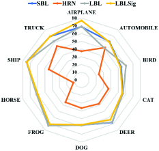
Figure 2: Comparisons of G-mean with SBL and HRN using MLP.

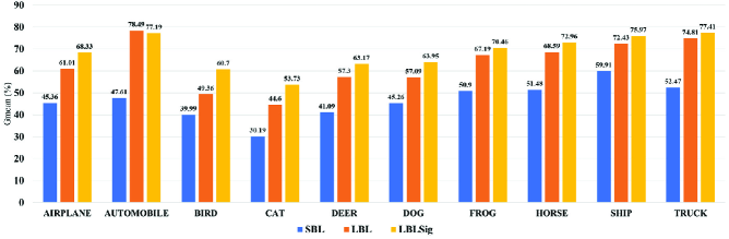
Figure 3: Comparisons of G-mean with SBL using OCITN.

TABLE II: Comparisons on SVHN using OCITN.

Target	AUC			Gmean
Digit	SBL	LBL	LBLSig	SBL	LBL	LBLSig
0	73.85	86.59	88.12	55.93	75.44	80.73
1	75.65	86.56	88.96	57.83	72.77	80.77
2	68.44	86.11	85.41	51.56	73.39	77.60
3	58.10	73.93	74.36	38.38	56.32	65.44
4	63.67	79.23	80.40	42.33	64.59	72.43
5	72.41	84.62	84.45	57.30	74.17	77.14
6	73.79	84.23	84.36	56.03	74.65	77.06
7	70.09	84.61	84.48	50.72	72.04	77.24
8	70.34	82.10	80.67	49.51	65.49	71.79
9	63.36	82.97	82.14	41.19	68.23	74.64
AVG	68.97	83.09	83.34	50.08	69.71	75.48

TABLE III: Comparisons of AUCs on non-image datasets.

Dataset	SBL	HRN	LBL	LBLSig
abalone	87.95	87.69	87.97	88.03
Arrhythmia	76.49	73.50	76.68	77.17
BASEHOCK	57.25	56.47	57.47	59.82
diabetes	72.47	69.77	71.91	73.04
Diabetic	63.36	62.74	65.45	63.68
ecoli	89.09	91.59	96.24	94.58
heart	83.51	82.39	82.72	85.61
leukemia	81.43	69.29	83.69	83.45
liver	58.79	61.25	58.65	61.91
magic	83.51	85.87	86.93	84.36
Online news	61.30	60.35	62.22	62.37
RCV1-4Class	78.27	54.84	79.67	79.05
Sonar	69.79	62.18	70.36	72.73
AVG	74.09	70.61	75.38	75.83

IV-C Comparisons with SOTA algorithms

TABLE IV: Comparisons of AUCs with the SOTA OCC algorithms.

Target	LSAR	OCGAN	HLS-OC	MOCCA	HRN	LBL∗	LBLSig∗
Class	[13]	[23]	[14]	[12]	[28]
AIRPLANE	73.5	75.7	73.7	66.0	77.3	76.38	78.03
AUTOMOBILE	58.0	53.1	74.4	74.6	69.9	87.93	87.29
BIRD	69.0	64.0	60.9	57.5	60.6	68.82	69.42
CAT	54.2	62.0	63.9	60.1	64.4	60.50	60.91
DEER	76.1	72.3	71.0	61.5	71.5	71.01	71.18
DOG	54.6	62.0	64.1	68.4	67.4	72.17	71.99
FROG	75.1	72.3	78.8	67.4	77.4	79.83	78.54
HORSE	53.5	57.5	70.6	72.1	64.9	80.82	81.59
SHIP	71.7	82.0	81.8	79.2	82.5	84.33	84.80
TRUCK	54.8	55.4	79.0	77.3	77.3	84.36	84.96
AVG	64.05	65.63	71.82	68.61	71.32	76.62	76.87

• *Conducted on OCITN

TABLE V: Comparisons of AUCs with PANDA-EWC using pretrained network.

Target	PANDA-EWC	LBLSig∗
Class	[30]
AIRPLANE	97.24	97.36
AUTOMOBILE	98.36	98.60
BIRD	93.20	93.23
CAT	90.08	90.03
DEER	97.29	97.38
DOG	94.35	94.13
FROG	97.31	97.78
HORSE	97.18	97.44
SHIP	97.33	97.73
TRUCK	97.13	97.68
AVG	95.95	96.14

• *Conducted on the PANDA structure.

In this section, comparisons on CIFAR10 with the latest SOTA OCC algorithms, including LSAR [13], OCGAN [23], HLS-OC [14], MOCCA [12] and HRN [28], are reported. The OCITN is chosen as the backbone to conduct our proposed LBL and LBLSig. The results are listed in Tabel IV and it can be seen that the best performance is obtained by the proposed LBL/LBLSig. Specially, the LBLSig achieves more than $12\%$, $10\%$, $4\%$, $8\%$ and $5\%$ increments of the average AUC over the LSAR, OCGAN, HLS-OC, MOCCA and HRN, respectively.

The recent researches show that the transfer learning can improve the OCC performance on images effectively [30, 31]. The proposed LBLSig is also demonstrated on the pretrained network. Following [30], the PANDA structure is adopted to conduct the proposed loss functions. In PANDA structure, the pretrained ResNet152 on ImageNet is used as the backbone and then fine-tuned by OCC loss functions. In this experiment, the PANDA with elastic weight consolidation regularization (PANDA-EWC), which is the main contribution of [30], is used for comparisons and the results of each class are obtained by runing the original code. The proposed LBLSig is only embedded into PANDA as the loss function for fine-tuning (without adding EWC) and other settings are all the same as [30]. It can be readily seen from Table V that the SOTA performance can be obtained by simply replacing the OCC loss of original PANDA with the proposed LBLSig.

V Conclusions

In this paper, two novel OCC loss functions named LBL and LBLSig were proposed. LBL employed the logarithmic barrier function to approximate the OCC objective smoothly. It assigned large gradients to the margin samples and thus derived more compact hypersphere. Due to the instability of the optimization of LBL, the LBLSig was further proposed by introducing a unilateral relaxation Sigmoid function. The LBLSig can be seen as the fusion of the MSE and the CE and the optimization of LBLSig was smoother owing to the unilateral relaxation Sigmoid function. The superior performance of the proposed LBL and LBLSig was experimentally verified in comparisons with several state-of-the-art OCC algorithms.

VI Supplementary Material

VI-A CIFAR10 and SVHN

The well-known CIFAR10 and SVHN are chosen to demonstrate the performance of the proposed LBL and LBLSig.

The CIFAR10⁵ is the frequently used dataset in the recent OCC algorithms [27, 28, 13, 23, 14, 12, 30, 31, 29] consisting of 50000 training samples and 10000 testing samples with $32\times 32$ color images from 10 classes, including airplane, automobile, bird, cat, deer, dog, frog, horse, ship and truck. There are 5000 images per class in training and 1000 images per class in testing. To conduct OCC, each class of the CIFAR10 is respectively chosen as the target class and the remaining classes are considered as outliers. For training dataset, only the chosen target class is used to train and the remaining classes are discarded. The total testing dataset is used to verify the model.

The SVHN⁶ is a real-world images including the street view house numbers $0-9$. There are 73257 digits for training and 26032 digits for testing and the cropped digits with $32\times 32$ color images are used. Similarly, each class of the SVHN is respectively chosen as the target class and the remaining classes are set to be outliers. Only target class is used to training model and the total testing dataset is used to verify the model.

VI-B Non-image Datasets

To further demonstrate the performance of the proposed methods, comparisons are condected on $13$ non-image datasets from the UCI Machine Learning Repository, the ASU feature selection datasets and LIBSVM database. Tabel VI gives the specifications of non-image datasets where the first class is set as the target and the remaining classes are considered as outliers.

TABLE VI: Specifications of non-image datasets.

Dataset	Training Data / Targets	Testing Data / Targets	No. of features
abalone7	2088 / 703	2089 / 704	8
Arrhythmia7	225 / 122	227 / 123	274
BASEHOCK8	1195 / 596	798 / 398	4862
diabetes9	383 / 252	385 / 253	8
Diabetic7	806 / 378	345 / 162	19
ecoli7	168 / 26	168 / 26	7
heart9	100 / 54	170 / 96	13
leukemia9	38 / 27	34 / 20	7129
liver7	172 / 72	173 / 73	6
magic7	10000 / 6430	9020 / 5902	10
Online news7	27751 / 12943	11893 / 5547	59
RCV1-4Class7	5775 / 1213	3850 / 809	29992
Sonar9	103 / 55	105 / 56	60

VI-C Implementation Detail Supplement

The proposed LBL and LBLSig are conducted on $4$ different networks for comparisons with SBL [27] and HRN [28], including DSLeNet in [27], MLP with $2$ hidden layers, OCITN in [29] and PANDA in [30]. The grid search method is employed to select the optimal hyperparameters for all algorithms and the settings have been detailed in the body. Besides, for LBLSig, the relaxation hyperparameter $Q$ is set to be 10 in this paper, and the radius $R$ is computed using the $0.9$-th quantiles

$$R={{Quantile}}\left({Dis\left({{\boldsymbol{\Phi}}({\bf{x}}_{i};{\boldsymbol{\mathcal{W}}}),{\bf{c}}}\right)},0.9\right).$$ (15)

Here ${Quantile}(\cdot,q)$ is carried out by the PyTorch function torch.quantile.

VI-D Some Supplements

In our opinion, ablation studies may obtain inconsistent results across different networks and datasets, rendering them meaningless and unconvincing. Ablation of $\theta$ is given in Fig. 4 for replying this comment, but it is insufficient to derive useful conclusions.

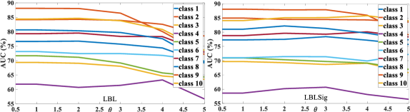
Figure 4: Ablation study of $\theta$.

TABLE VII: Comparisons on MVTecAD.

Algorithms/Metric	AVG. AUC
MSP-AD [44]	98.1
CFLOW-AD [45]	98.26
PatchCore [46]	99.1
Proposed LBL	98.89

In our view, MVTecAD [47] may be challenging in anomaly segmentation but it is a toy dataset in OCC due to its easy data construction. For example, LBL with 2-layer MLP is conducted on MVTecAD and results are listed in Tabel VII. LBL with simple MLP achieved the second-best and even close to 99$\%$ AUC.

References

- [1] G. Pang, C. Shen, L. Cao, and A. V. D. Hengel, “Deep learning for anomaly detection: A review,” ACM Computing Surveys (CSUR), vol. 54, no. 2, pp. 1–38, 2021.
- [2] B. Schölkopf, J. C. Platt, J. Shawe-Taylor, A. J. Smola, and R. C. Williamson, “Estimating the support of a high-dimensional distribution,” Neural Computation, vol. 13, no. 7, pp. 1443–1471, 2001.
- [3] D. M. Tax and R. P. Duin, “Support vector data description,” Machine Learning, vol. 54, no. 1, pp. 45–66, 2004.
- [4] I. Goodfellow, Y. Bengio, and A. Courville, Deep Learning. MIT Press, 2016, http://www.deeplearningbook.org.
- [5] S. Pidhorskyi, R. Almohsen, and G. Doretto, “Generative probabilistic novelty detection with adversarial autoencoders,” Advances in neural information processing systems, vol. 31, 2018.
- [6] C. Zhou and R. C. Paffenroth, “Anomaly detection with robust deep autoencoders,” in Proceedings of the 23rd ACM SIGKDD international conference on knowledge discovery and data mining, 2017, pp. 665–674.
- [7] D. Gong, L. Liu, V. Le, B. Saha, M. R. Mansour, S. Venkatesh, and A. v. d. Hengel, “Memorizing normality to detect anomaly: Memory-augmented deep autoencoder for unsupervised anomaly detection,” in Proceedings of the IEEE/CVF International Conference on Computer Vision, 2019, pp. 1705–1714.
- [8] X. Wang, Y. Du, S. Lin, P. Cui, Y. Shen, and Y. Yang, “advae: A self-adversarial variational autoencoder with gaussian anomaly prior knowledge for anomaly detection,” Knowledge-Based Systems, vol. 190, p. 105187, 2020.
- [9] M. Sakurada and T. Yairi, “Anomaly Detection Using Autoencoders with Nonlinear Dimensionality Reduction,” in Proceedings of MLSDA 2014 2nd Workshop on Machine Learning for Sensory Data Analysis, 2014, pp. 4–11.
- [10] J. An and S. Cho, “Variational Autoencoder based Anomaly Detection using Reconstruction Probability,” Special Lecture on IE, vol. 2, no. 1, 2015.
- [11] J. Chen, S. Sathe, C. Aggarwal, and D. Turaga, “Outlier Detection with Autoencoder Ensembles,” in Proceedings of 2017 SIAM International Conference on Data Mining, 2017, pp. 90–98.
- [12] F. V. Massoli, F. Falchi, A. Kantarci, S. Akti, H. K. Ekenel, and G. Amato, “MOCCA: Multilayer One-Class Classification for Anomaly Detection,” IEEE Transactions on Neural Networks and Learning Systems, vol. 33, no. 6, pp. 2313–2323, 2022.
- [13] D. Abati, A. Porrello, S. Calderara, and R. Cucchiara, “Latent space autoregression for novelty detection,” in Proceedings of IEEE Conference on Computer Vision and Pattern Recognition, 2019, pp. 481–490.
- [14] T. Wang, J. Cao, X. Lai, and Q. M. Wu, “Hierarchical One-Class Classifier with Within-Class Scatter-Based Autoencoders,” IEEE Transactions on Neural Networks and Learning Systems, vol. 32, no. 8, pp. 3770–3776, 2021.
- [15] J. T. Andrews, E. J. Morton, and L. D. Griffin, “Detecting Anomalous Data Using Auto-Encoders,” International Journal of Machine Learning and Computing, vol. 6, no. 1, p. 21, 2016.
- [16] D. Xu, E. Ricci, Y. Yan, J. Song, and N. Sebe, “Learning Deep Representations of Appearance and Motion for Anomalous Event Detection,” arXiv preprint arXiv:1510.01553, 2015.
- [17] S. M. Erfani, S. Rajasegarar, S. Karunasekera, and C. Leckie, “High-dimensional and large-scale anomaly detection using a linear one-class SVM with deep learning,” Pattern Recognition, vol. 58, pp. 121–134, 2016.
- [18] T. Schlegl, P. Seeböck, S. M. Waldstein, U. Schmidt-Erfurth, and G. Langs, “Unsupervised Anomaly Detection with Generative Adversarial Networks to Guide Marker Discovery,” in Proceedings of International Conference on Information Processing in Medical Imaging, 2017, pp. 146–157.
- [19] M. Sabokrou, M. Khalooei, M. Fathy, and E. Adeli, “Adversarially learned one-class classifier for novelty detection,” in Proceedings of the IEEE conference on computer vision and pattern recognition, 2018, pp. 3379–3388.
- [20] M. Z. Zaheer, J.-h. Lee, M. Astrid, and S.-I. Lee, “Old is gold: Redefining the adversarially learned one-class classifier training paradigm,” in Proceedings of the IEEE/CVF Conference on Computer Vision and Pattern Recognition, 2020, pp. 14 183–14 193.
- [21] D. Abati, A. Porrello, S. Calderara, and R. Cucchiara, “Latent space autoregression for novelty detection,” in Proceedings of the IEEE/CVF conference on computer vision and pattern recognition, 2019, pp. 481–490.
- [22] M. Sabokrou, M. Khalooei, M. Fathy, and E. Adeli, “Adversarially learned one-class classifier for novelty detection,” in Proceedings of the IEEE conference on computer vision and pattern recognition, 2018, pp. 3379–3388.
- [23] P. Perera, R. Nallapati, and B. Xiang, “OCGAN: One-class novelty detection using gans with constrained latent representations,” in Proceedings of IEEE Conference on Computer Vision and Pattern Recognition, 2019, pp. 2898–2906.
- [24] T. Schlegl, P. Seeböck, S. M. Waldstein, G. Langs, and U. Schmidt-Erfurth, “f-anogan: Fast unsupervised anomaly detection with generative adversarial networks,” Medical image analysis, vol. 54, pp. 30–44, 2019.
- [25] I. Golan and R. El-Yaniv, “Deep Anomaly Detection Using Geometric Transformations,” in Proceedings of Advances in Neural Information Processing Systems, vol. 31, 2018.
- [26] J. Wang and A. Cherian, “GODS: Generalized One-class Discriminative Subspaces for Anomaly Detection,” in Proceedings of the IEEE International Conference on Computer Vision, 2019, pp. 8201–8211.
- [27] L. Ruff, R. A. Vandermeulen, N. Görnitz, L. Deecke, S. A. Siddiqui, A. Binder, E. Müller, and M. Kloft, “Deep One-Class Classification,” in Proceedings of the International Conference on Machine Learning, 2018, pp. 4390–4399.
- [28] W. Hu, M. Wang, Q. Qin, J. Ma, and B. Liu, “HRN: A Holistic Approach to One Class Learning,” in Advances in Neural Information Processing Systems, vol. 33, 2020, pp. 19 111–19 124.
- [29] T. Hayashi, H. Fujita, and A. Hernandez-Matamoros, “Less complexity one-class classification approach using construction error of convolutional image transformation network,” Information Sciences, vol. 560, pp. 217–234, 2021.
- [30] T. Reiss, N. Cohen, L. Bergman, and Y. Hoshen, “PANDA: Adapting Pretrained Features for Anomaly Detection and Segmentation,” in Proceedings of the IEEE/CVF Conference on Computer Vision and Pattern Recognition, 2021, pp. 2806–2814.
- [31] M. J. Cohen and S. Avidan, “Transformaly-two (feature spaces) are better than one,” in Proceedings of the IEEE/CVF Conference on Computer Vision and Pattern Recognition, 2022, pp. 4060–4069.
- [32] Y. Li, Y. Song, and J. Luo, “Improving Pairwise Ranking for Multi-Label Image Classification,” in Proceedings of the IEEE Conference on Computer Vision and Pattern Recognition, 2017, pp. 3617–3625.
- [33] S. Boyd and L. Vandenberghe, Convex Optimization. Cambridge university press, 2004.
- [34] D. Tax, “Ddtools, the data description toolbox for matlab,” Jan 2018, version 2.1.3.
- [35] Q. Leng, H. Qi, J. Miao, W. Zhu, and G. Su, “One-Class Classification with Extreme Learning Machine,” Mathematical Problems in Engineering, vol. 2015, 2015.
- [36] A. Iosifidis, V. Mygdalis, A. Tefas, and I. Pitas, “One-Class Classification Based on Extreme Learning and Geometric Class Information,” Neural Processing Letters, vol. 45, no. 2, pp. 577–592, 2017.
- [37] C. Gautam, A. Tiwari, and A. Iosifidis, “Minimum Variance-Embedded Multi-layer Kernel Ridge Regression for One-class Classification,” in Proceedings of the 2018 IEEE Symposium Series on Computational Intelligence, SSCI 2018, 2018, pp. 389–396.
- [38] H. Dai, J. Cao, T. Wang, M. Deng, and Z. Yang, “Multilayer one-class extreme learning machine,” Neural Networks, vol. 115, pp. 11–22, 2019.
- [39] T. Wang, J. Cao, X. Lai, and Q. M. Wu, “Within-Class Scatter Constraint Based Randomized Autoencoder for One-Class Classification,” in Proceedings of 2nd China Symposium on Cognitive Computing and Hybrid Intelligence, CCHI 2019, 2019, pp. 111–116.
- [40] T. Wang, J. Cao, H. Dai, B. Lei, and H. Zeng, “Robust Maximum Mixture Correntropy Criterion based One-Class Classification Algorithm,” IEEE Intelligent Systems, pp. 1–7, 2021.
- [41] X. Cui, J. Cao, T. Wang, and X. Lai, “Robust randomized autoencoder and correntropy criterion-based one-class classification,” IEEE Transactions on Circuits and Systems II: Express Briefs, vol. 68, no. 4, pp. 1517–1521, 2021.
- [42] I. Gulrajani, F. Ahmed, M. Arjovsky, V. Dumoulin, and A. C. Courville, “Improved training of wasserstein gans,” in Advances in Neural Information Processing Systems, I. Guyon, U. V. Luxburg, S. Bengio, H. Wallach, R. Fergus, S. Vishwanathan, and R. Garnett, Eds., vol. 30. Curran Associates, Inc., 2017.
- [43] J. M. Lobo, A. Jiménez-valverde, and R. Real, “AUC: A misleading measure of the performance of predictive distribution models,” Global Ecology and Biogeography, vol. 17, no. 2, pp. 145–151, 2008.
- [44] C.-C. Tsai, T.-H. Wu, and S.-H. Lai, “Multi-scale patch-based representation learning for image anomaly detection and segmentation,” in Proceedings of the IEEE/CVF Winter Conference on Applications of Computer Vision, 2022, pp. 3992–4000.
- [45] D. Gudovskiy, S. Ishizaka, and K. Kozuka, “Cflow-ad: Real-time unsupervised anomaly detection with localization via conditional normalizing flows,” in Proceedings of the IEEE/CVF Winter Conference on Applications of Computer Vision, 2022, pp. 98–107.
- [46] K. Roth, L. Pemula, J. Zepeda, B. Schölkopf, T. Brox, and P. Gehler, “Towards total recall in industrial anomaly detection,” in Proceedings of the IEEE/CVF Conference on Computer Vision and Pattern Recognition, 2022, pp. 14 318–14 328.
- [47] P. Bergmann, M. Fauser, D. Sattlegger, and C. Steger, “MVTec AD – A Comprehensive Real-World Dataset for Unsupervised Anomaly Detection,” in Proceedings of the IEEE/CVF Conference on Computer Vision and Pattern Recognition (CVPR), June 2019, pp. 9592–9600.