Fisher-Rao distance and pullback SPD cone distances between multivariate normal distributions111A preliminary version of this work appeared as “Fisher-Rao and pullback Hilbert cone distances on the multivariate Gaussian manifold with applications to simplification and quantization of mixtures,” at the 2nd Annual Topology, Algebra, and Geometry in Machine Learning Workshop (TAG-ML) of ICML’23.

Frank Nielsen
 
Sony Computer Science Laboratories Inc.
Tokyo, Japan
0000-0001-5728-0726
Abstract

Data sets of multivariate normal distributions abound in many scientific areas like diffusion tensor imaging, structure tensor computer vision, radar signal processing, machine learning, etc. In order to process those normal data sets for downstream tasks like filtering, classification or clustering, one needs to define proper notions of dissimilarities between normals and paths joining them. The Fisher-Rao distance defined as the Riemannian geodesic distance induced by the Fisher information metric is such a principled metric distance which however is not known in closed-form excepts for a few particular cases. In this work, we first report a fast and robust method to approximate the Fisher-Rao distance between multivariate normal distributions with a guaranteed 1+ϵ1italic-ϵ1+\epsilon factor for any ϵ>0italic-ϵ0\epsilon>0. Second, we introduce a class of distances based on diffeomorphic embeddings of the normal manifold into a submanifold of the higher-dimensional symmetric positive-definite cone corresponding to the manifold of centered normal distributions. We show that the projective Hilbert distance on the cone yields a metric on the embedded normal submanifold and we pullback that cone distance with its associated straight line Hilbert cone geodesics to obtain a distance and smooth paths between normal distributions. Compared to the Fisher-Rao distance approximation, the pullback Hilbert cone distance is computationally light since it requires to compute only the extreme minimal and maximal eigenvalues of matrices. Finally, we show how to use those distances in clustering tasks.

1 Introduction

Data sets of multivariate normal distributions (MVNs) are increasing frequent in many scientific areas like medical imaging (diffusion tensor imaging [40]), computer vision (image segmentation [22] or structure tensor imaging [63]), signal processing (covariance matrices [11] in radar or brain computer interfaces [10]), and machine learning (Gaussian mixtures or kernel density estimators [28]). These data sets can be viewed as (weighted) point sets on a Gaussian manifold and Riemannian and information-geometric structures [67, 77] on that manifold allows one to define geodesics and distances or divergences which allows on to build algorithms like filtering, classification, clustering or optimization techniques [74, 1, 43]. For example, we may simplify a Gaussian mixture model [28, 37, 79] (GMM) with n𝑛n components by viewing the mixture as a weighted point set and simplify the mixture by clustering the point set into k𝑘k clusters using k𝑘k-means or k𝑘k-medioids [28] (as known as discrete k𝑘k-means). We may also consider n𝑛n GMMs with potentially different components and build a codebook of all mixture components to quantize and compress the representation of these GMMs. In this work, we consider two kinds of metric distances and metric geodesics: The Fisher-Rao distance [69] and a new distance obtained by pulling back the Hilbert cone projective distance on an embedding of the Gaussian manifold into the higher-dimensional symmetric positive-definite matrix cone [20].

The paper is organized as follows: In Section 2, we recall the Fisher-Rao geodesic distance and mention its lack of general closed-form formula on the Gaussian manifold. We then build on a recent breakthrough which studied the MVN Fisher-Rao geodesics [49]2.2) to design an approximation method which upper bounds the true Fisher-Rao distance with guaranteed (1+ϵ)1italic-ϵ(1+\epsilon) precision for any ϵ>0italic-ϵ0\epsilon>0 (Theorem 2.2 in §2.3). We present applications to simplification and quantization of GMMs in Section 3 using fast clustering methods relying on nearest neighbor query data structures [76] and smallest enclosing balls in metric spaces. In Section 4, we introduce the novel pullback Hilbert cone distance which is fast to compute and enjoys simple expression of geodesics.

2 Fisher-Rao geodesics and distances

A normal distribution N(μ,Σ)𝑁𝜇ΣN(\mu,\Sigma) has probability density function (pdf) pμ,Σ(x)subscript𝑝𝜇Σ𝑥p_{\mu,\Sigma}(x) defined on the full support dsuperscript𝑑\mathbb{R}^{d} given by:

pμ,Σ(x)=(2π)d2det(Σ)exp((xμ)Σ1(xμ)2).subscript𝑝𝜇Σ𝑥superscript2𝜋𝑑2detΣsuperscript𝑥𝜇topsuperscriptΣ1𝑥𝜇2\displaystyle p_{\mu,\Sigma}(x)=\frac{(2\pi)^{-\frac{d}{2}}}{\sqrt{\mathrm{det}(\Sigma)}}\exp\left(-\frac{(x-\mu)^{\top}\Sigma^{-1}(x-\mu)}{2}\right).

Consider the statistical model consisting of all d𝑑d-variate normal distributions:

𝒩(d)={N(λ):λ=(μ,Σ)Λ(d)=d×Sym+(d,)},𝒩𝑑conditional-set𝑁𝜆𝜆𝜇ΣΛ𝑑superscript𝑑subscriptSym𝑑\mathcal{N}(d)=\left\{N(\lambda)\ :\ \lambda=(\mu,\Sigma)\in\Lambda(d)=\mathbb{R}^{d}\times\mathrm{Sym}_{+}(d,\mathbb{R})\right\},

where Sym+(d,)subscriptSym𝑑\mathrm{Sym}_{+}(d,\mathbb{R}) denote the set of d×d𝑑𝑑d\times d positive-definite matrices. The dimension of 𝒩(d)𝒩𝑑\mathcal{N}(d) is m=dim(Λ(d))=d+d(d+1)2=d(d+3)2𝑚dimΛ𝑑𝑑𝑑𝑑12𝑑𝑑32m=\mathrm{dim}(\Lambda(d))=d+\frac{d(d+1)}{2}=\frac{d(d+3)}{2}. When the dimension is clear from context, we omit to specify the dimension and write 𝒩𝒩\mathcal{N} for short.

Let lλ(x)=logpλ(x)subscript𝑙𝜆𝑥subscript𝑝𝜆𝑥l_{\lambda}(x)=\log p_{\lambda}(x) denote the log-likelihood function. The MVN model is both identifiable (bijection between λ𝜆\lambda and pλsubscript𝑝𝜆p_{\lambda}) and regular [19, 5], i.e., the Fisher information matrix I(θ)=Eθ[2lθ(x)]𝐼𝜃subscript𝐸𝜃delimited-[]superscript2subscript𝑙𝜃𝑥I(\theta)=-E_{\theta}[\nabla^{2}l_{\theta}(x)] is positive-definite and defines a Riemannian metric gFishersubscript𝑔Fisherg_{\mathrm{Fisher}} called the Fisher information metric. The Riemannian manifold (𝒩,gFisher)𝒩subscript𝑔Fisher(\mathcal{N},g_{\mathrm{Fisher}}) is called the Fisher-Rao Gaussian manifold with squared infinitesimal length element [67] dsFisher2dsuperscriptsubscript𝑠Fisher2\mathrm{d}s_{\mathrm{Fisher}}^{2} at (μ,Σ)𝜇Σ(\mu,\Sigma) given by:

dsFisher2=dμΣ1dμ+12tr((Σ1dΣ)2),dsuperscriptsubscript𝑠Fisher2dsuperscript𝜇topsuperscriptΣ1d𝜇12trsuperscriptsuperscriptΣ1dΣ2\mathrm{d}s_{\mathrm{Fisher}}^{2}=\mathrm{d}\mu^{\top}\Sigma^{-1}\mathrm{d}\mu+\frac{1}{2}\mathrm{tr}\left(\left(\Sigma^{-1}\mathrm{d}\Sigma\right)^{2}\right),

where dμdd𝜇superscript𝑑\mathrm{d}\mu\in\mathbb{R}^{d} and dΣSym(d,)dΣSym𝑑\mathrm{d}\Sigma\in\mathrm{Sym}(d,\mathbb{R}) (vector space of symmetric d×d𝑑𝑑d\times d matrices).

The Fisher-Rao length of a smooth curve c(t)𝑐𝑡c(t) with t[a,b]𝑡𝑎𝑏t\in[a,b] is defined by integrating the infinitesimal Fisher-Rao length element along the curve: Len(c)=abdsFisher(c(t))dtLen𝑐superscriptsubscript𝑎𝑏differential-dsubscript𝑠Fisher𝑐𝑡differential-d𝑡\mathrm{Len}(c)=\int_{a}^{b}\mathrm{d}s_{\mathrm{Fisher}}(c(t))\,\mathrm{d}t, and the Fisher-Rao distance [44, 64] between N0=N(μ0,Σ0)subscript𝑁0𝑁subscript𝜇0subscriptΣ0N_{0}=N(\mu_{0},\Sigma_{0}) and N1=N(μ1,Σ1)subscript𝑁1𝑁subscript𝜇1subscriptΣ1N_{1}=N(\mu_{1},\Sigma_{1}) is the geodesic distance on (𝒩,gFisher)𝒩subscript𝑔Fisher(\mathcal{N},g_{\mathrm{Fisher}}), i.e., the length of the Riemannian geodesic γFR𝒩(N0,N1;t)superscriptsubscript𝛾FR𝒩subscript𝑁0subscript𝑁1𝑡\gamma_{\mathrm{FR}}^{\mathcal{N}}(N_{0},N_{1};t):

ρFR(N0,N1)=01dsFisher(γFR𝒩(N0,N1;t))dt.subscript𝜌FRsubscript𝑁0subscript𝑁1superscriptsubscript01differential-dsubscript𝑠Fishersuperscriptsubscript𝛾FR𝒩subscript𝑁0subscript𝑁1𝑡differential-d𝑡\rho_{\mathrm{FR}}(N_{0},N_{1})=\int_{0}^{1}\mathrm{d}s_{\mathrm{Fisher}}(\gamma_{\mathrm{FR}}^{\mathcal{N}}(N_{0},N_{1};t))\,\mathrm{d}t. (1)

In Riemannian geometry [36], geodesics with boundary conditions N0=γFR𝒩(N0,N1;0)subscript𝑁0superscriptsubscript𝛾FR𝒩subscript𝑁0subscript𝑁10N_{0}=\gamma_{\mathrm{FR}}^{\mathcal{N}}(N_{0},N_{1};0) and N1=γFR(N0,N1;1)subscript𝑁1subscript𝛾FRsubscript𝑁0subscript𝑁11N_{1}=\gamma_{\mathrm{FR}}(N_{0},N_{1};1) are length minimizing curves among all curves c(t)𝑐𝑡c(t) satisfying c(0)=N(μ0,Σ0)𝑐0𝑁subscript𝜇0subscriptΣ0c(0)=N(\mu_{0},\Sigma_{0}) and c(1)=N(μ1,Σ1)𝑐1𝑁subscript𝜇1subscriptΣ1c(1)=N(\mu_{1},\Sigma_{1}):

ρFR(N0,N1)=infc(t)c(0)=pμ0,Σ0c(1)=pμ1,Σ1{Len(c)}.subscript𝜌FRsubscript𝑁0subscript𝑁1subscriptinfimum𝑐𝑡𝑐0subscript𝑝subscript𝜇0subscriptΣ0𝑐1subscript𝑝subscript𝜇1subscriptΣ1Len𝑐\rho_{\mathrm{FR}}(N_{0},N_{1})=\inf_{\begin{subarray}{c}c(t)\\ c(0)=p_{\mu_{0},\Sigma_{0}}\\ c(1)=p_{\mu_{1},\Sigma_{1}}\end{subarray}}\,\left\{\mathrm{Len}(c)\right\}.

Riemannian geodesics are parameterized by (normalized) arc length t𝑡t which ensures that

ρ(γρ(P0,P1;s),γρ(P0,P1;t))=|st|ρ(P0,P1).𝜌subscript𝛾𝜌subscript𝑃0subscript𝑃1𝑠subscript𝛾𝜌subscript𝑃0subscript𝑃1𝑡𝑠𝑡𝜌subscript𝑃0subscript𝑃1\rho(\gamma_{\rho}(P_{0},P_{1};s),\gamma_{\rho}(P_{0},P_{1};t))=|s-t|\,\rho(P_{0},P_{1}). (2)

More generally, geodesics in differential geometry [19] are auto-parallel curves with respect to an affine connection \nabla: γ˙γ˙=0subscript˙𝛾˙𝛾0\nabla_{\dot{\gamma}}\dot{\gamma}=0, where ˙=ddt˙absent𝑑d𝑡\dot{\ }=\frac{d}{\mathrm{d}t} and XYsubscript𝑋𝑌\nabla_{X}Y is the covariant derivative induced by the connection. In Riemannian geometry, the default connection is the unique Levi-Civita metric connection [36] gsuperscript𝑔\nabla^{g} induced by the metric g𝑔g.

In general, the Fisher-Rao distance between MVNs is not known in closed-form [62, 56]. However, there are two main cases where closed-form formula are known:

  • The case d=1𝑑1d=1: The Fisher-Rao distance between univariate normal distributions [78] N0=N(μ0,σ02)subscript𝑁0𝑁subscript𝜇0superscriptsubscript𝜎02N_{0}=N(\mu_{0},\sigma_{0}^{2}) and N1=N(μ1,σ12)subscript𝑁1𝑁subscript𝜇1superscriptsubscript𝜎12N_{1}=N(\mu_{1},\sigma_{1}^{2}) is

    ρ𝒩(N0,N1)=2log(1+Δ(μ0,σ0;μ1,σ1)1Δ(μ0,σ0;μ1,σ1)),subscript𝜌𝒩subscript𝑁0subscript𝑁121Δsubscript𝜇0subscript𝜎0subscript𝜇1subscript𝜎11Δsubscript𝜇0subscript𝜎0subscript𝜇1subscript𝜎1\rho_{\mathcal{N}}(N_{0},N_{1})=\sqrt{2}\log\left(\frac{1+\Delta(\mu_{0},\sigma_{0};\mu_{1},\sigma_{1})}{1-\Delta(\mu_{0},\sigma_{0};\mu_{1},\sigma_{1})}\right), (3)

    where for (a,b,c,d)4\{0}𝑎𝑏𝑐𝑑\superscript40(a,b,c,d)\in\mathbb{R}^{4}\backslash\{0\},

    Δ(a,b;c,d)=(ca)2+2(db)2(ca)2+2(d+b)2Δ𝑎𝑏𝑐𝑑superscript𝑐𝑎22superscript𝑑𝑏2superscript𝑐𝑎22superscript𝑑𝑏2\Delta(a,b;c,d)=\sqrt{\frac{(c-a)^{2}+2(d-b)^{2}}{(c-a)^{2}+2(d+b)^{2}}} (4)

    is a Möbius distance [17].

  • The case where MVNs N0subscript𝑁0N_{0} and N1subscript𝑁1N_{1} share the same mean [46, 67], i.e., they belong to some submanifold 𝒩μ={N(μ,Σ):ΣSym+(d,)}subscript𝒩𝜇conditional-set𝑁𝜇ΣΣsubscriptSym𝑑\mathcal{N}_{\mu}=\{N(\mu,\Sigma)\ :\ \Sigma\in\mathrm{Sym}_{+}(d,\mathbb{R})\}. When μ=0𝜇0\mu=0, we let 𝒫(d)=𝒩0(d)𝒫𝑑subscript𝒩0𝑑\mathcal{P}(d)=\mathcal{N}_{0}(d). We have:

    ρ𝒩μ(N0,N1)subscript𝜌subscript𝒩𝜇subscript𝑁0subscript𝑁1\displaystyle\rho_{\mathcal{N}_{\mu}}(N_{0},N_{1}) =\displaystyle= 12i=1dlog2λi(Σ012Σ1Σ012),12superscriptsubscript𝑖1𝑑superscript2subscript𝜆𝑖superscriptsubscriptΣ012subscriptΣ1superscriptsubscriptΣ012\displaystyle\sqrt{\frac{1}{2}\sum_{i=1}^{d}\log^{2}\lambda_{i}(\Sigma_{0}^{-\frac{1}{2}}\Sigma_{1}\Sigma_{0}^{-\frac{1}{2}})}, (5)

    where λi(M)subscript𝜆𝑖𝑀\lambda_{i}(M) denotes the i𝑖i-th largest eigenvalue of matrix M𝑀M. Observe that matrix Σ01Σ1superscriptsubscriptΣ01subscriptΣ1\Sigma_{0}^{-1}\Sigma_{1} may not be symmetric but Σ012Σ1Σ012superscriptsubscriptΣ012subscriptΣ1superscriptsubscriptΣ012\Sigma_{0}^{-\frac{1}{2}}\Sigma_{1}\Sigma_{0}^{-\frac{1}{2}} is always SPD and λi(Σ01Σ1)=λi(Σ012Σ1Σ012)subscript𝜆𝑖superscriptsubscriptΣ01subscriptΣ1subscript𝜆𝑖superscriptsubscriptΣ012subscriptΣ1superscriptsubscriptΣ012\lambda_{i}(\Sigma_{0}^{-1}\Sigma_{1})=\lambda_{i}(\Sigma_{0}^{-\frac{1}{2}}\Sigma_{1}\Sigma_{0}^{-\frac{1}{2}}). The submanifolds 𝒩μsubscript𝒩𝜇\mathcal{N}_{\mu} are totally geodesic in 𝒩𝒩\mathcal{N}, and the Fisher-Rao geodesics are known in closed form: γFR𝒩(N0,N1;t)=N(μ,Σt)superscriptsubscript𝛾FR𝒩subscript𝑁0subscript𝑁1𝑡𝑁𝜇subscriptΣ𝑡\gamma_{\mathrm{FR}}^{\mathcal{N}}(N_{0},N_{1};t)=N(\mu,\Sigma_{t}) with

    ΣtsubscriptΣ𝑡\displaystyle\Sigma_{t} =\displaystyle= Σ012(Σ012Σ1Σ012)tΣ012.superscriptsubscriptΣ012superscriptsuperscriptsubscriptΣ012subscriptΣ1superscriptsubscriptΣ012𝑡superscriptsubscriptΣ012\displaystyle\Sigma_{0}^{\frac{1}{2}}\,(\Sigma_{0}^{-\frac{1}{2}}\Sigma_{1}\Sigma_{0}^{-\frac{1}{2}})^{t}\,\Sigma_{0}^{\frac{1}{2}}. (6)

    The geodesic γ(Σ0,Σ1;t)=Σt𝛾subscriptΣ0subscriptΣ1𝑡subscriptΣ𝑡\gamma(\Sigma_{0},\Sigma_{1};t)=\Sigma_{t} (with t[0,1]𝑡01t\in[0,1]) midpoint is thus

    γ(Σ0,Σ1;12)=Σ12=Σ012(Σ012Σ1Σ012)12Σ012.𝛾subscriptΣ0subscriptΣ112subscriptΣ12superscriptsubscriptΣ012superscriptsuperscriptsubscriptΣ012subscriptΣ1superscriptsubscriptΣ01212superscriptsubscriptΣ012\gamma(\Sigma_{0},\Sigma_{1};\frac{1}{2})=\Sigma_{\frac{1}{2}}=\Sigma_{0}^{\frac{1}{2}}\,(\Sigma_{0}^{-\frac{1}{2}}\Sigma_{1}\Sigma_{0}^{-\frac{1}{2}})^{\frac{1}{2}}\,\Sigma_{0}^{\frac{1}{2}}.

    See also Appendix C.

Notice that all submanifolds 𝒩μsubscript𝒩𝜇\mathcal{N}_{\mu} are non-positive curvature manifolds (NPC) [16, 25], i.e. sectional curvatures are non-positive. However, 𝒩(d)𝒩𝑑\mathcal{N}(d) is not a NPC manifold when d>1𝑑1d>1 since some sectional curvatures can be positive [67]. NPC property is important for designing optimization algorithms on manifolds with guaranteed convergence [25]. In a NPC manifold (M,g)𝑀𝑔(M,g), we can write the Riemannian distance using the Riemannian logarithm map Logp:MTpM:subscriptLog𝑝𝑀subscript𝑇𝑝𝑀{\mathrm{Log}}_{p}:M\rightarrow T_{p}M: ρg(p1,p2)=Logp1(p2)p1subscript𝜌𝑔subscript𝑝1subscript𝑝2subscriptnormsubscriptLogsubscript𝑝1subscript𝑝2subscript𝑝1\rho_{g}(p_{1},p_{2})=\|{\mathrm{Log}}_{p_{1}}(p_{2})\|_{p_{1}}, where vp=gp(v,v)subscriptnorm𝑣𝑝subscript𝑔𝑝𝑣𝑣\|v\|_{p}=\sqrt{g_{p}(v,v)}. On the NPC SPD cone Sym+(d,)subscriptSym𝑑\mathrm{Sym}_{+}(d,\mathbb{R}) equipped with the trace metric [54, 29]

gPtrace(P1,P2):=tr(P1P1P1P2),assignsuperscriptsubscript𝑔𝑃tracesubscript𝑃1subscript𝑃2trsuperscript𝑃1subscript𝑃1superscript𝑃1subscript𝑃2g_{P}^{\mathrm{trace}}(P_{1},P_{2}):=\mathrm{tr}(P^{-1}P_{1}P^{-1}P_{2}),

the length element at P𝑃P is dsP=P12dPP12Fdsubscript𝑠𝑃subscriptnormsuperscript𝑃12d𝑃superscript𝑃12𝐹\mathrm{d}s_{P}=\|P^{-\frac{1}{2}}\mathrm{d}PP^{-\frac{1}{2}}\|_{F}, and the Riemannian logarithm map is expressed using the matrix logarithm LogLog{\mathrm{Log}}, and we have

ρgtrace(P1,P2)=LogP1(P2)P1=Log(P11P2)F,subscript𝜌subscript𝑔tracesubscript𝑃1subscript𝑃2subscriptnormsubscriptLogsubscript𝑃1subscript𝑃2subscript𝑃1subscriptnormLogsuperscriptsubscript𝑃11subscript𝑃2𝐹\rho_{g_{\mathrm{trace}}}(P_{1},P_{2})=\|{\mathrm{Log}}_{P_{1}}(P_{2})\|_{P_{1}}=\|{\mathrm{Log}}(P_{1}^{-1}P_{2})\|_{F},

where XF=X,XF=i,jXij2subscriptnorm𝑋𝐹subscript𝑋𝑋𝐹subscript𝑖𝑗superscriptsubscript𝑋𝑖𝑗2\|X\|_{F}=\sqrt{{\langle X,X\rangle}_{F}}=\sqrt{\sum_{i,j}X_{ij}^{2}} is the Frobenius norm induced by the Frobenius inner product: A,BF=tr(AB)subscript𝐴𝐵𝐹trsuperscript𝐴top𝐵{\langle A,B\rangle}_{F}=\mathrm{tr}(A^{\top}B) (Hilbert-Schmidt inner product). The Fröbenius norm can be calculated in quadratic time as MF=i,j=1dmij2subscriptnorm𝑀𝐹superscriptsubscript𝑖𝑗1𝑑superscriptsubscript𝑚𝑖𝑗2\|M\|_{F}=\sqrt{\sum_{i,j=1}^{d}m_{ij}^{2}} for a d×d𝑑𝑑d\times d matrix M=[mij]𝑀delimited-[]subscript𝑚𝑖𝑗M=[m_{ij}], and is equivalent to the 2subscript2\ell_{2} norm on the vectorization of M𝑀M: MF=vec(M)2subscriptnorm𝑀𝐹subscriptnormvec𝑀2\|M\|_{F}=\|\mathrm{vec}(M)\|_{2}, where vec(M)=[m11,,m1d,,md1,,mdd]d2vec𝑀superscriptsubscript𝑚11subscript𝑚1𝑑subscript𝑚𝑑1subscript𝑚𝑑𝑑topsuperscriptsuperscript𝑑2\mathrm{vec}(M)=[m_{11},\ldots,m_{1d},\ldots,m_{d1},\ldots,m_{dd}]^{\top}\in\mathbb{R}^{d^{2}}. The SPD cone is also a Bruhat-Tits space [52].

Historically, the SPD Riemannian trace metric distance was studied by Siegel [66] in the wider context of the complex manifold of symmetric complex square matrices with positive-definite imaginary part: The so-called Siegel upper half space [33] which generalizes the Poincaré upper plane. It was shown recently that the Siegel upper half space is NPC [18]. Another popular distance in machine learning in the Wasserstein distance for which the underlying geometry on the Gaussian space was studied in [71].

2.1 Invariance under action of the positive affine group

The length element dsFisherdsubscript𝑠Fisher\mathrm{d}s_{\mathrm{Fisher}} is invariant under the action of the positive affine group [31, 32]

Aff+(d,):={(a,A):ad,AGL+(d,)},assignsubscriptAff𝑑conditional-set𝑎𝐴formulae-sequence𝑎superscript𝑑𝐴subscriptGL𝑑\mathrm{Aff}_{+}(d,\mathbb{R}){:=}\left\{(a,A)\ :\ a\in\mathbb{R}^{d},A\in\mathrm{GL}_{+}(d,\mathbb{R})\right\},

where GL+(d,)subscriptGL𝑑\mathrm{GL}_{+}(d,\mathbb{R}) denotes the group of d×d𝑑𝑑d\times d matrices with positive determinant. The group identity element of Aff+(d,)subscriptAff𝑑\mathrm{Aff}_{+}(d,\mathbb{R}) is e=(0,I)𝑒0𝐼e=(0,I) and the group operation is (a1,A1).(a2,A2)=(a1+A1a2,A1A2)formulae-sequencesubscript𝑎1subscript𝐴1subscript𝑎2subscript𝐴2subscript𝑎1subscript𝐴1subscript𝑎2subscript𝐴1subscript𝐴2(a_{1},A_{1}).(a_{2},A_{2})=(a_{1}+A_{1}a_{2},A_{1}A_{2}) with inverse operation (a,A)1=(A1a,A1)superscript𝑎𝐴1superscript𝐴1𝑎superscript𝐴1(a,A)^{-1}=(-A^{-1}a,A^{-1})). The positive affine group may be handled as a matrix group by mapping elements (a,A)𝑎𝐴(a,A) to (d+1)×(d+1)𝑑1𝑑1(d+1)\times(d+1) matrices M(a,A):=[Aa01]assignsubscript𝑀𝑎𝐴delimited-[]𝐴𝑎01M_{(a,A)}{:=}{\left[\begin{array}[]{ll}A&a\cr 0&1\end{array}\right]}. Then the matrix group operation is the matrix multiplication and inverse operation is given by the matrix inverse. Let us consider the following group action (denoted by the dot .) of the positive affine group on the Gaussian manifold 𝒩𝒩\mathcal{N}:

(a,A).N(μ,Σ)=N(a+Aμ,AΣA).formulae-sequence𝑎𝐴𝑁𝜇Σ𝑁𝑎𝐴𝜇𝐴Σsuperscript𝐴top(a,A).N(\mu,\Sigma)=N(a+A\mu,A\Sigma A^{\top}).

This action corresponds to the affine transformation of random variables: Y=a+AXN(a+Aμ,AΣA)𝑌𝑎𝐴𝑋similar-to𝑁𝑎𝐴𝜇𝐴Σsuperscript𝐴topY=a+AX\sim N(a+A\mu,A\Sigma A^{\top}) where XN(μ,Σ)similar-to𝑋𝑁𝜇ΣX\sim N(\mu,\Sigma). The statistical model 𝒩𝒩\mathcal{N} can thus be interpreted as a group with identity element the standard MVN Nstd=N(0,I)subscript𝑁std𝑁0𝐼N_{\mathrm{std}}=N(0,I): 𝒩(d)={(a,A).Nstd:(a,A)Aff+(d)}\mathcal{N}(d)=\left\{(a,A).N_{\mathrm{std}}\ :\ (a,A)\in\mathrm{Aff}_{+}(d)\right\}. We get a Lie group differential structure on 𝒩𝒩\mathcal{N} [51] which moreover extends to a statistical Lie group structure in information geometry [34].

It can be checked that the Fisher-Rao length element is invariant under the action of Aff+(d,)subscriptAff𝑑\mathrm{Aff}_{+}(d,\mathbb{R}) and therefore the Fisher-Rao distance is also invariant: ρFR((a,A).N0:(a,A).N1)=ρFR(N0,N1)\rho_{\mathrm{FR}}((a,A).N_{0}:(a,A).N_{1})=\rho_{\mathrm{FR}}(N_{0},N_{1}). It follows that the Fisher-Rao geodesics in 𝒩𝒩\mathcal{N} are equivariant [31, 49] γFR𝒩(B.N0,B.N1;t)=B.γFR𝒩(N0,N1;t)\gamma_{\mathrm{FR}}^{\mathcal{N}}(B.N_{0},B.N_{1};t)=B.\gamma_{\mathrm{FR}}^{\mathcal{N}}(N_{0},N_{1};t) for any BAff+(d,)𝐵subscriptAff𝑑B\in\mathrm{Aff}_{+}(d,\mathbb{R}) and we can therefore consider without loss of generality that N0subscript𝑁0N_{0} is the standard normal distribution and N1N1=N(Σ012(μ1,μ0),Σ012Σ1Σ012)subscript𝑁1superscriptsubscript𝑁1𝑁superscriptsubscriptΣ012subscript𝜇1subscript𝜇0superscriptsubscriptΣ012subscriptΣ1superscriptsubscriptΣ012N_{1}\rightarrow N_{1}^{\prime}=N\left(\Sigma_{0}^{-\frac{1}{2}}(\mu_{1},-\mu_{0}),\Sigma_{0}^{-\frac{1}{2}}\Sigma_{1}\Sigma_{0}^{-\frac{1}{2}}\right).

2.2 Fisher-Rao geodesics with boundary conditions

The Fisher-Rao geodesic Ordinary Differential Equation (ODE) for MVNs was first studied by Skovgaard [67]:

{μ¨Σ˙Σ1μ˙=0,Σ¨+μ˙μ˙Σ˙Σ1Σ˙=0.cases¨𝜇˙ΣsuperscriptΣ1˙𝜇0¨Σ˙𝜇superscript˙𝜇top˙ΣsuperscriptΣ1˙Σ0\left\{\begin{array}[]{lcl}\ddot{\mu}-\dot{\Sigma}\Sigma^{-1}\dot{\mu}&=&0,\\ \ddot{\Sigma}+\dot{\mu}\dot{\mu}^{\top}-\dot{\Sigma}\Sigma^{-1}\dot{\Sigma}&=&0.\end{array}\right. (7)
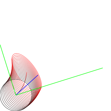
Refer to caption Refer to caption
(a) (b)
Refer to caption Refer to caption
(c) (d)
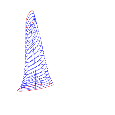
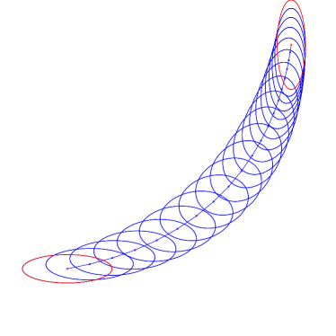
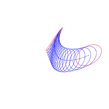
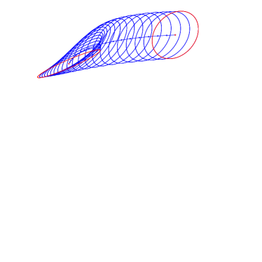
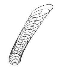
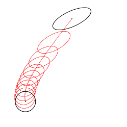
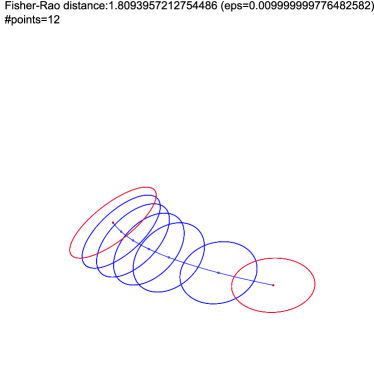
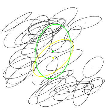
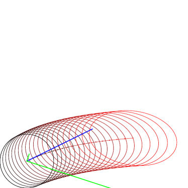
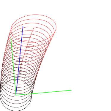
Figure 1: Some Fisher-Rao geodesics γFR𝒩(N0,N1)superscriptsubscript𝛾FR𝒩subscript𝑁0subscript𝑁1\gamma_{\mathrm{FR}}^{\mathcal{N}}(N_{0},N_{1}) with boundary conditions (bivariate normals N0subscript𝑁0N_{0} and N1subscript𝑁1N_{1} indicated by ellipsoids displayed in red) on the bivariate Gaussian manifold. The sample space 2superscript2\mathbb{R}^{2} is visualized for the range [0.3,1.2]×[0.3,1.2]0.31.20.31.2[-0.3,1.2]\times[-0.3,1.2].

Eriksen [31] first reported a solution of the geodesic equation with initial conditions: That is Fisher-Rao geodesics emanating from source N0subscript𝑁0N_{0} with initial prescribed tangent vector v0=γ˙(0)subscript𝑣0˙𝛾0v_{0}=\dot{\gamma}(0) in the tangent plane TN0subscript𝑇subscript𝑁0T_{N_{0}}. The initial tangent vector v0=(a0,B0)TN0subscript𝑣0subscript𝑎0subscript𝐵0subscript𝑇subscript𝑁0v_{0}=(a_{0},B_{0})\in T_{N_{0}} consists of a vector part a0subscript𝑎0a_{0} and a symmetric matrix part B0subscript𝐵0B_{0}. Eriksen’s solution required to compute a matrix exponential of a matrix of size (2d+1)×(2d+1)2𝑑12𝑑1(2d+1)\times(2d+1) and the inner use of square matrices of dimension 2d+12𝑑12d+1 was not fully geometrically elucidated [45]. See Appendix A.1 for details of Eriksen’s method which gives a pregeodesic γ¯FR𝒩(N0,v0;u)superscriptsubscript¯𝛾FR𝒩subscript𝑁0subscript𝑣0𝑢\underline{\gamma}_{\mathrm{FR}}^{\mathcal{N}}(N_{0},v_{0};u) and not a geodesic γFR𝒩(N0,v0;t)superscriptsubscript𝛾FR𝒩subscript𝑁0subscript𝑣0𝑡{\gamma}_{\mathrm{FR}}^{\mathcal{N}}(N_{0},v_{0};t) which is parameterized by arclength (constant speed). Geodesics can be obtained from pregeodesics by smooth reparameterization with an auxiliary function u()𝑢u(\cdot): γFR𝒩(N0,v0;t)=γ¯FR𝒩(N0,v0;u(t))superscriptsubscript𝛾FR𝒩subscript𝑁0subscript𝑣0𝑡superscriptsubscript¯𝛾FR𝒩subscript𝑁0subscript𝑣0𝑢𝑡{\gamma}_{\mathrm{FR}}^{\mathcal{N}}(N_{0},v_{0};t)=\underline{\gamma}_{\mathrm{FR}}^{\mathcal{N}}(N_{0},v_{0};u(t)).

Calvo and Oller [21] later studied a more general differential equation system than in Eq. 7 and reported a closed-form solution without using extra dimensions (see Appendix A.2). For many years, the Fisher-Rao geodesics with boundary conditions N0subscript𝑁0N_{0} and N1subscript𝑁1N_{1} were not known in closed-form and had to be approximated using geodesic shooting methods [40, 61]: Those geodesic shooting methods were time consuming and numerically unstable, thus limiting their use in applications [40]. A recent breakthrough by Kobayashi [49] full explains and extends geometrically the rationale of Eriksen and obtains a method to compute in closed-form the Fisher-Rao geodesic with boundary conditions. Namely, Kobayashi [49] proved that the Fisher-Rao geodesics can be obtained by a Riemannian submersion of horizontal geodesics of the non-compact Riemannian symmetric space of dimension 2d+12𝑑12d+1. We report concisely below the recipe which we extracted from Kobayashi’s principled geometric method to derive Nt=γFR𝒩(N0,N1;t)subscript𝑁𝑡superscriptsubscript𝛾FR𝒩subscript𝑁0subscript𝑁1𝑡N_{t}=\gamma_{\mathrm{FR}}^{\mathcal{N}}(N_{0},N_{1};t) as follows:
 

Algorithm 1. Fisher-Rao geodesic Nt=N(μ(t),Σ(t))=γFR𝒩(N0,N1;t)subscript𝑁𝑡𝑁𝜇𝑡Σ𝑡superscriptsubscript𝛾FR𝒩subscript𝑁0subscript𝑁1𝑡N_{t}=N(\mu(t),\Sigma(t))=\gamma_{\mathrm{FR}}^{\mathcal{N}}(N_{0},N_{1};t): For i{0,1}𝑖01i\in\{0,1\}, let Gi=MiDiMisubscript𝐺𝑖subscript𝑀𝑖subscript𝐷𝑖superscriptsubscript𝑀𝑖topG_{i}=M_{i}\,D_{i}\,M_{i}^{\top}, where Misubscript𝑀𝑖\displaystyle M_{i} =\displaystyle= [Σi10001000Σi],delimited-[]subscriptsuperscriptΣ1𝑖0001000subscriptΣ𝑖\displaystyle{\left[\begin{array}[]{lll}\Sigma^{-1}_{i}&0&0\cr 0&1&0\cr 0&0&\Sigma_{i}\end{array}\right]}, (11) Disubscript𝐷𝑖\displaystyle D_{i} =\displaystyle= [Id00μi100μiId],delimited-[]subscript𝐼𝑑00superscriptsubscript𝜇𝑖top100subscript𝜇𝑖subscript𝐼𝑑\displaystyle{\left[\begin{array}[]{lll}I_{d}&0&0\cr\mu_{i}^{\top}&1&0\cr 0&-\mu_{i}&I_{d}\end{array}\right]}, (15) where Idsubscript𝐼𝑑I_{d} denotes the identity matrix of shape d×d𝑑𝑑d\times d. That is, matrices G0subscript𝐺0G_{0} and G1Sym+(2d+1,)subscript𝐺1subscriptSym2𝑑1G_{1}\in\mathrm{Sym}_{+}(2d+1,\mathbb{R}) can be expressed by block Cholesky factorizations. Consider the Riemannian geodesic in Sym+(2d+1,)subscriptSym2𝑑1\mathrm{Sym}_{+}(2d+1,\mathbb{R}) with respect to the trace metric: G(t)=G012(G012G1G012)tG012.𝐺𝑡superscriptsubscript𝐺012superscriptsuperscriptsubscript𝐺012subscript𝐺1superscriptsubscript𝐺012𝑡superscriptsubscript𝐺012G(t)=G_{0}^{\frac{1}{2}}\,\left(G_{0}^{-\frac{1}{2}}G_{1}G_{0}^{-\frac{1}{2}}\right)^{t}\,G_{0}^{\frac{1}{2}}. In order to compute the matrix power Gpsuperscript𝐺𝑝G^{p} for p𝑝p\in\mathbb{R}, we first calculate the Singular Value Decomposition (SVD) of G𝐺G: G=OLO𝐺𝑂𝐿superscript𝑂topG=O\,L\,O^{\top} (where O𝑂O is an orthogonal matrix and L=diag(λ1,,λ2d+1)𝐿diagsubscript𝜆1subscript𝜆2𝑑1L=\mathrm{diag}(\lambda_{1},\ldots,\lambda_{2d+1}) a diagonal matrix) and then get the matrix power as Gp=OLpOsuperscript𝐺𝑝𝑂superscript𝐿𝑝superscript𝑂topG^{p}=O\,L^{p}\,O^{\top} with Lp=diag(λ1p,,λ2d+1p)superscript𝐿𝑝diagsuperscriptsubscript𝜆1𝑝superscriptsubscript𝜆2𝑑1𝑝L^{p}=\mathrm{diag}(\lambda_{1}^{p},\ldots,\lambda_{2d+1}^{p}). Retrieve N(t)=γFR𝒩(N0,N1;t)=N(μ(t),Σ(t))𝑁𝑡superscriptsubscript𝛾FR𝒩subscript𝑁0subscript𝑁1𝑡𝑁𝜇𝑡Σ𝑡N(t)=\gamma_{\mathrm{FR}}^{\mathcal{N}}(N_{0},N_{1};t)=N(\mu(t),\Sigma(t)) from G(t)𝐺𝑡G(t): Σ(t)Σ𝑡\displaystyle\Sigma(t) =\displaystyle= [G(t)]1:d,1:d1,superscriptsubscriptdelimited-[]𝐺𝑡:1𝑑1:𝑑1\displaystyle[G(t)]_{1:d,1:d}^{-1}, (16) μ(t)𝜇𝑡\displaystyle\mu(t) =\displaystyle= Σ(t)[G(t)]1:d,d+1,Σ𝑡subscriptdelimited-[]𝐺𝑡:1𝑑𝑑1\displaystyle\Sigma(t)\,[G(t)]_{1:d,d+1}, (17) where [G]1:d,1:dsubscriptdelimited-[]𝐺:1𝑑1:𝑑[G]_{1:d,1:d} denotes the block matrix with rows and columns ranging from 111 to d𝑑d extracted from (2d+1)×(2d+1)2𝑑12𝑑1(2d+1)\times(2d+1) matrix G𝐺G, and [G]1:d,d+1subscriptdelimited-[]𝐺:1𝑑𝑑1[G]_{1:d,d+1} is similarly the column vector of dsuperscript𝑑\mathbb{R}^{d} extracted from G𝐺G.

Note that this technique also proves that the MVN geodesics are unique although 𝒩𝒩\mathcal{N} is not NPC. It is proven in [34] that the Gaussian manifold admits a solvable Lie group and hence is diffeomorphic to some Euclidean space. Figure 1 displays several bivariate normal Fisher-Rao geodesics with boundary conditions obtained by implementing this method [49]. We display N(μ,Σ)𝑁𝜇ΣN(\mu,\Sigma) by an ellipse ={μ+Lx:x2=1}conditional-set𝜇𝐿𝑥subscriptnorm𝑥21\mathcal{E}=\{\mu+Lx\ :\ \|x\|_{2}=1\} where Σ=LLΣ𝐿superscript𝐿top\Sigma=LL^{\top} (Cholesky decomposition).

2.3 Fisher-Rao distances

2.3.1 Approximating Fisher-Rao lengths of curves

The previous section reported the closed-form solutions for the Fisher-Rao geodesics γFR𝒩(N0,N1;t)superscriptsubscript𝛾FR𝒩subscript𝑁0subscript𝑁1𝑡\gamma_{\mathrm{FR}}^{\mathcal{N}}(N_{0},N_{1};t). We shall now explain a method to approximate their lengths and hence the Fisher-Rao distances:

ρFR(N0,N1)=Len(γFR𝒩(N0,N1;t)).subscript𝜌FRsubscript𝑁0subscript𝑁1Lensuperscriptsubscript𝛾FR𝒩subscript𝑁0subscript𝑁1𝑡\rho_{\mathrm{FR}}(N_{0},N_{1})=\mathrm{Len}(\gamma_{\mathrm{FR}}^{\mathcal{N}}(N_{0},N_{1};t)).

Consider discretizing regularly t[0,1]𝑡01t\in[0,1] using T+1𝑇1T+1 steps: 0T=0,1T,,T1T,TT=1formulae-sequence0𝑇01𝑇𝑇1𝑇𝑇𝑇1\frac{0}{T}=0,\frac{1}{T},\ldots,\frac{T-1}{T},\frac{T}{T}=1. Since geodesics are totally 1D submanifolds, we have

ρFR(N0,N1)=i=0T1ρFR(γFR(NiT,Ni+1T)).subscript𝜌FRsubscript𝑁0subscript𝑁1superscriptsubscript𝑖0𝑇1subscript𝜌FRsubscript𝛾FRsubscript𝑁𝑖𝑇subscript𝑁𝑖1𝑇\rho_{\mathrm{FR}}(N_{0},N_{1})=\sum_{i=0}^{T-1}\rho_{\mathrm{FR}}(\gamma_{\mathrm{FR}}\left(N_{\frac{i}{T}},N_{\frac{i+1}{T}}\right)).

By choosing T𝑇T large enough, we have N=NiT𝑁subscript𝑁𝑖𝑇N=N_{\frac{i}{T}} close to N=Ni+1Tsuperscript𝑁subscript𝑁𝑖1𝑇N^{\prime}=N_{\frac{i+1}{T}}, and we can approximate the geodesic distance as follows:

ρFR(N,N)dsFisher(N)2f′′(1)If(N,N),subscript𝜌FR𝑁superscript𝑁dsubscript𝑠Fisher𝑁2superscript𝑓′′1subscript𝐼𝑓𝑁superscript𝑁\rho_{\mathrm{FR}}(N,N^{\prime})\approx\mathrm{d}s_{\mathrm{Fisher}}(N)\approx\sqrt{\frac{2}{f^{\prime\prime}(1)}I_{f}(N,N^{\prime})},

where If(p,q)subscript𝐼𝑓𝑝𝑞I_{f}(p,q) is any f𝑓f-divergence [3, 27] between pdfs p(x)𝑝𝑥p(x) and q(x)𝑞𝑥q(x) induced by a strictly convex generator f(u)𝑓𝑢f(u) satisfying f(1)=0𝑓10f(1)=0:

If(p,q)=p(x)f(q(x)p(x))dx.subscript𝐼𝑓𝑝𝑞𝑝𝑥𝑓𝑞𝑥𝑝𝑥differential-d𝑥I_{f}(p,q)=\int p(x)f\left(\frac{q(x)}{p(x)}\right)\,\mathrm{d}x.

Indeed, we have for two close distributions pθsubscript𝑝𝜃p_{\theta} and pθ+dθsubscript𝑝𝜃d𝜃p_{\theta+\mathrm{d}\theta} [5]: If(pθ,pθ+dθ)f′′(1)2dsFisher2subscript𝐼𝑓subscript𝑝𝜃subscript𝑝𝜃d𝜃superscript𝑓′′12dsubscriptsuperscript𝑠2FisherI_{f}(p_{\theta},p_{\theta+\mathrm{d}\theta})\approx\frac{f^{\prime\prime}(1)}{2}\mathrm{d}s^{2}_{\mathrm{Fisher}}.

We choose the Jeffreys f𝑓f-divergence which is the arithmetic symmetrization of the Kullback-Leibler divergence obtained for the generator fJ(u)=(u1)logusubscript𝑓𝐽𝑢𝑢1𝑢f_{J}(u)=(u-1)\log u with fJ′′(1)=2superscriptsubscript𝑓𝐽′′12f_{J}^{\prime\prime}(1)=2. It follows that DJ(N1,N2)=IfJ(N1,N2)=tr(Σ21Σ1+Σ11Σ22I)+(μ2μ1)Σ11+Σ212(μ2μ1)subscript𝐷𝐽subscript𝑁1subscript𝑁2subscript𝐼subscript𝑓𝐽subscript𝑁1subscript𝑁2trsuperscriptsubscriptΣ21subscriptΣ1superscriptsubscriptΣ11subscriptΣ22𝐼superscriptsubscript𝜇2subscript𝜇1topsuperscriptsubscriptΣ11superscriptsubscriptΣ212subscript𝜇2subscript𝜇1D_{J}(N_{1},N_{2})=I_{f_{J}}(N_{1},N_{2})=\mathrm{tr}\left(\frac{\Sigma_{2}^{-1}\Sigma_{1}+\Sigma_{1}^{-1}\Sigma_{2}}{2}-I\right)+(\mu_{2}-\mu_{1})^{\top}\frac{\Sigma_{1}^{-1}+\Sigma_{2}^{-1}}{2}(\mu_{2}-\mu_{1}).

Thus we get the following overall approximation of the Fisher-Rao distance:

ρ~T(N0,N1)=i=0T1DJ(NiT,Ni+1T)ρFR(N0,N1).subscript~𝜌𝑇subscript𝑁0subscript𝑁1superscriptsubscript𝑖0𝑇1subscript𝐷𝐽subscript𝑁𝑖𝑇subscript𝑁𝑖1𝑇subscript𝜌FRsubscript𝑁0subscript𝑁1\tilde{\rho}_{T}(N_{0},N_{1})=\sum_{i=0}^{T-1}\sqrt{D_{J}\left(N_{\frac{i}{T}},N_{\frac{i+1}{T}}\right)}\approx\rho_{\mathrm{FR}}(N_{0},N_{1}). (18)

In [35], the authors choose dsFisher(p)=2DKL(pθ,pθ+dθ)dsubscript𝑠Fisher𝑝2subscript𝐷KLsubscript𝑝𝜃subscript𝑝𝜃d𝜃\mathrm{d}s_{\mathrm{Fisher}}(p)=\sqrt{2D_{\mathrm{KL}}(p_{\theta},p_{\theta+\mathrm{d}\theta})} where DKL=IfKLsubscript𝐷KLsubscript𝐼subscript𝑓KLD_{\mathrm{KL}}=I_{f_{\mathrm{KL}}} is the Kullback-Leibler divergence, a f𝑓f-divergence obtained for fKL(u)=logusubscript𝑓KL𝑢𝑢f_{\mathrm{KL}}(u)=-\log u.

Property 1 (Fisher-Rao upper bound).

The Fisher-Rao distance between normal distributions is upper bounded by the square root of the Jeffreys divergence: ρFR(N0,N1)DJ(N0,N1)subscript𝜌FRsubscript𝑁0subscript𝑁1subscript𝐷𝐽subscript𝑁0subscript𝑁1\rho_{\mathrm{FR}}(N_{0},N_{1})\leq\sqrt{D_{J}(N_{0},N_{1})}.

The proof can be found in many places, e.g. [39, 5, 65]. Yet we report another proof in Appendix B.

Notice that we have ρFR(N0,N1)ρ~T(N0,N1)subscript𝜌FRsubscript𝑁0subscript𝑁1subscript~𝜌𝑇subscript𝑁0subscript𝑁1\rho_{\mathrm{FR}}(N_{0},N_{1})\leq\tilde{\rho}_{T}(N_{0},N_{1}) for all T>1𝑇1T>1. Define the energy of a curve c(t)𝑐𝑡c(t) with t[a,b]𝑡𝑎𝑏t\in[a,b] by E(c)=abdsFisher2(t)dt𝐸𝑐superscriptsubscript𝑎𝑏differential-dsubscriptsuperscript𝑠2Fisher𝑡differential-d𝑡E(c)=\int_{a}^{b}\mathrm{d}s^{2}_{\mathrm{Fisher}}(t)\mathrm{d}t. We have

E(γe𝒩(N0,N1;t))=E(γm𝒩(N0,N1;t))=DJ(N0,N1),𝐸superscriptsubscript𝛾𝑒𝒩subscript𝑁0subscript𝑁1𝑡𝐸superscriptsubscript𝛾𝑚𝒩subscript𝑁0subscript𝑁1𝑡subscript𝐷𝐽subscript𝑁0subscript𝑁1E(\gamma_{e}^{\mathcal{N}}(N_{0},N_{1};t))=E(\gamma_{m}^{\mathcal{N}}(N_{0},N_{1};t))=D_{J}(N_{0},N_{1}),

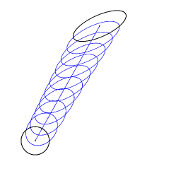
where γe𝒩(N0,N1;t)=N(μte,Σte)superscriptsubscript𝛾𝑒𝒩subscript𝑁0subscript𝑁1𝑡𝑁superscriptsubscript𝜇𝑡𝑒superscriptsubscriptΣ𝑡𝑒\gamma_{e}^{\mathcal{N}}(N_{0},N_{1};t)=N(\mu_{t}^{e},\Sigma_{t}^{e}) and γm𝒩(N0,N1;t)=N(μtm,Σtm)superscriptsubscript𝛾𝑚𝒩subscript𝑁0subscript𝑁1𝑡𝑁superscriptsubscript𝜇𝑡𝑚superscriptsubscriptΣ𝑡𝑚\gamma_{m}^{\mathcal{N}}(N_{0},N_{1};t)=N(\mu_{t}^{m},\Sigma_{t}^{m}) are the exponential and mixture geodesics in information geometry [77] given by μtm=μ¯tsuperscriptsubscript𝜇𝑡𝑚subscript¯𝜇𝑡\mu_{t}^{m}=\bar{\mu}_{t} and Σtm=Σ¯t+tμ1μ1+(1t)μ2μ2μ¯tμ¯tsuperscriptsubscriptΣ𝑡𝑚subscript¯Σ𝑡𝑡subscript𝜇1superscriptsubscript𝜇1top1𝑡subscript𝜇2superscriptsubscript𝜇2topsubscript¯𝜇𝑡superscriptsubscript¯𝜇𝑡top\Sigma_{t}^{m}=\bar{\Sigma}_{t}+t\mu_{1}\mu_{1}^{\top}+(1-t)\mu_{2}\mu_{2}^{\top}-\bar{\mu}_{t}\bar{\mu}_{t}^{\top} where μ¯t=tμ1+(1t)μ2subscript¯𝜇𝑡𝑡subscript𝜇11𝑡subscript𝜇2\bar{\mu}_{t}=t\mu_{1}+(1-t)\mu_{2} and Σ¯t=tΣ1+(1t)Σ2subscript¯Σ𝑡𝑡subscriptΣ11𝑡subscriptΣ2\bar{\Sigma}_{t}=t\Sigma_{1}+(1-t)\Sigma_{2}, and μte=Σ¯tH(tΣ11μ1+(1t)Σ21μ2)superscriptsubscript𝜇𝑡𝑒superscriptsubscript¯Σ𝑡𝐻𝑡superscriptsubscriptΣ11subscript𝜇11𝑡superscriptsubscriptΣ21subscript𝜇2\mu_{t}^{e}=\bar{\Sigma}_{t}^{H}(t\Sigma_{1}^{-1}\mu_{1}+(1-t)\Sigma_{2}^{-1}\mu_{2}) and Σte=Σ¯tHsuperscriptsubscriptΣ𝑡𝑒subscriptsuperscript¯Σ𝐻𝑡\Sigma_{t}^{e}=\bar{\Sigma}^{H}_{t} where Σ¯tH=(tΣ11+(1t)Σ21)1subscriptsuperscript¯Σ𝐻𝑡superscript𝑡superscriptsubscriptΣ111𝑡superscriptsubscriptΣ211\bar{\Sigma}^{H}_{t}=(t\Sigma_{1}^{-1}+(1-t)\Sigma_{2}^{-1})^{-1} is the matrix harmonic mean. See Figure 2. The mixture, Fisher-Rao, and exponential geodesics are α𝛼\alpha-connection geodesics [34] for α=1𝛼1\alpha=-1, α=0𝛼0\alpha=0 and α=1𝛼1\alpha=1, respectively. Notice that these e/m geodesics are computationally less intensive to evaluate than the Fisher-Rao geodesics.
Refer to caption Refer to caption Refer to caption
mixture geodesic γm𝒩superscriptsubscript𝛾𝑚𝒩\gamma_{m}^{\mathcal{N}} Fisher-Rao geodesic γ𝒩FRsuperscriptsubscript𝛾𝒩FR\gamma_{\mathcal{N}}^{\mathrm{FR}} exponential geodesic γe𝒩subscriptsuperscript𝛾𝒩𝑒\gamma^{\mathcal{N}}_{e}
Figure 2: Visualizing geodesics with respect to the mixture, Levi-Civita (Fisher-Rao), and exponential connections.

Since the upper bound of Property 1 is tight infinitesimally, we get in the limit convergence to the Fisher-Rao distance:

limTρ~T(N0,N1)=ρFR(N0,N1).subscript𝑇subscript~𝜌𝑇subscript𝑁0subscript𝑁1subscript𝜌FRsubscript𝑁0subscript𝑁1\lim_{T\rightarrow\infty}\tilde{\rho}_{T}(N_{0},N_{1})=\rho_{\mathrm{FR}}(N_{0},N_{1}).
Example 1.

Let us consider the example of Han and Park [40] (displayed in Figure 1(b)):

N0=N([00],[1000.1])subscript𝑁0𝑁delimited-[]00delimited-[]1000.1N_{0}=N\left({\left[\begin{array}[]{l}0\cr 0\end{array}\right]},{\left[\begin{array}[]{ll}1&0\cr 0&0.1\end{array}\right]}\right) and N1=N([11],[0.1001])subscript𝑁1𝑁delimited-[]11delimited-[]0.1001N_{1}=N\left({\left[\begin{array}[]{l}1\cr 1\end{array}\right]},{\left[\begin{array}[]{ll}0.1&0\cr 0&1\end{array}\right]}\right). The time consuming geodesic shooting algorithm of [40] evaluates the Fisher-Rao distance to ρ𝒩(N0,N1)3.1329subscript𝜌𝒩subscript𝑁0subscript𝑁13.1329\rho_{\mathcal{N}}(N_{0},N_{1})\approx 3.1329. We get the following approximations: ρ~T(N0,N1)=3.1996subscript~𝜌𝑇subscript𝑁0subscript𝑁13.1996\tilde{\rho}_{T}(N_{0},N_{1})=3.1996 for T=100𝑇100T=100. See Figure 3 for the convergence curve of ρ~T(N0,N1)subscript~𝜌𝑇subscript𝑁0subscript𝑁1\tilde{\rho}_{T}(N_{0},N_{1}) as a function of T𝑇T.

  3   3.2   3.4   3.6   3.8   4   4.2   4.4   0   10   20   30    40    50    60    70    80    90   100     ρ~Tsubscript~𝜌𝑇\tilde{\rho}_{T}T𝑇TFisher-Rao distance approximations                                                                                                                                                                      ++++++++++++++++++++++++++++++++++++++++++++++++++++++++++++++++++++++++++++++++++++++++++++++++++++++++++++++++++++++++++++++++++++++++++++++++++++++++++++++++++++++++++++++++++++++++++++++++++++++++++     
Figure 3: Convergence of ρ~T(N0,N1)subscript~𝜌𝑇subscript𝑁0subscript𝑁1\tilde{\rho}_{T}(N_{0},N_{1}) to ρFR(N0,N1)subscript𝜌FRsubscript𝑁0subscript𝑁1\rho_{\mathrm{FR}}(N_{0},N_{1}).

A lower bound for the Fisher-Rao MVN distance between MVNs was given in [20] by using a Fisher isometric embedding into the SPD cone of dimension d+1𝑑1d+1. Calvo and Oller [20] showed that mapping N=N(μ,Σ)𝑁𝑁𝜇ΣN=N(\mu,\Sigma) by

𝒩¯=f(N):=[Σ+μμμμ1]𝒫(d+1),¯𝒩𝑓𝑁assigndelimited-[]Σ𝜇superscript𝜇top𝜇superscript𝜇top1𝒫𝑑1{\overline{\mathcal{N}}}=f(N){:=}{\left[\begin{array}[]{ll}\Sigma+\mu\mu^{\top}&\mu\cr\mu^{\top}&1\end{array}\right]}\in\mathcal{P}(d+1), (19)

embeds the Gaussian manifold into a submanifold 𝒩¯¯𝒩\overline{\mathcal{N}} in the SPD cone 𝒫(d+1)𝒫𝑑1\mathcal{P}(d+1) of codimension 111. Moreoever, when 𝒫(d+1)𝒫𝑑1\mathcal{P}(d+1) is equipped with half the trace metric 12gtrace12subscript𝑔trace\frac{1}{2}g_{\mathrm{trace}}, the embedded MVN submanifold is Fisher isometric. However, the submanifold 𝒩¯¯𝒩\overline{\mathcal{N}} is not totally geodesic. Thus by taking the Riemannian SPD distance in 𝒫(d+1)𝒫𝑑1\mathcal{P}(d+1) induced by 12gtrace12subscript𝑔trace\frac{1}{2}g_{\mathrm{trace}}, we get a lower bound on the Fisher-Rao distance:

ρCO(N0,N1)=12i=1d+1log2λi(𝒩¯012𝒩¯1𝒩¯012).subscript𝜌COsubscript𝑁0subscript𝑁112superscriptsubscript𝑖1𝑑1superscript2subscript𝜆𝑖superscriptsubscript¯𝒩012subscript¯𝒩1superscriptsubscript¯𝒩012\displaystyle\rho_{\mathrm{CO}}(N_{0},N_{1})=\frac{1}{\sqrt{2}}\sum_{i=1}^{d+1}\log^{2}\lambda_{i}({\overline{\mathcal{N}}}_{0}^{-\frac{1}{2}}{\overline{\mathcal{N}}}_{1}{\overline{\mathcal{N}}}_{0}^{-\frac{1}{2}}).
Proposition 2.1.

A lower bound on the Fisher-Rao distance between N0=N(μ0,Σ0)subscript𝑁0𝑁subscript𝜇0subscriptΣ0N_{0}=N(\mu_{0},\Sigma_{0}) and N1=N(μ1,Σ1)subscript𝑁1𝑁subscript𝜇1subscriptΣ1N_{1}=N(\mu_{1},\Sigma_{1}) is

ρCO(N0,N1)=12i=1d+1log2λi(𝒩¯012𝒩¯1𝒩¯012),subscript𝜌COsubscript𝑁0subscript𝑁112superscriptsubscript𝑖1𝑑1superscript2subscript𝜆𝑖superscriptsubscript¯𝒩012subscript¯𝒩1superscriptsubscript¯𝒩012\rho_{\mathrm{CO}}(N_{0},N_{1})=\frac{1}{\sqrt{2}}\sum_{i=1}^{d+1}\log^{2}\lambda_{i}({\overline{\mathcal{N}}}_{0}^{-\frac{1}{2}}{\overline{\mathcal{N}}}_{1}{\overline{\mathcal{N}}}_{0}^{-\frac{1}{2}}),

where 𝒩¯i=[Σi+μiμiμiμi1]subscript¯𝒩𝑖delimited-[]subscriptΣ𝑖subscript𝜇𝑖superscriptsubscript𝜇𝑖topsubscript𝜇𝑖superscriptsubscript𝜇𝑖top1{\overline{\mathcal{N}}}_{i}={\left[\begin{array}[]{ll}\Sigma_{i}+\mu_{i}\mu_{i}^{\top}&\mu_{i}\cr\mu_{i}^{\top}&1\end{array}\right]} for i{0,1}𝑖01i\in\{0,1\}, and the λi(M)subscript𝜆𝑖𝑀\lambda_{i}(M)’s denote the eigenvalues of matrix M𝑀M.

2.3.2 A guaranteed (1+ϵ)1italic-ϵ(1+\epsilon)-approximation of the Fisher-Rao MVN distance

Using the lower and upper bounds on the Fisher-Rao distance and the closed-form solution for the Fisher-Rao geodesics with boundary value conditions, we can design a guaranteed (1+ϵ)1italic-ϵ(1+\epsilon)-approximation recursive algorithm for the Fisher-Rao MVN distance as follows:
Refer to caption Refer to caption
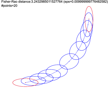
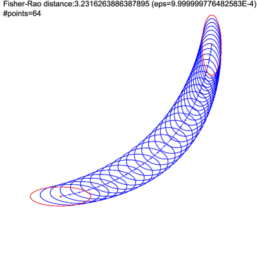
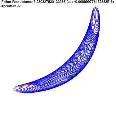
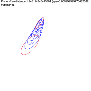
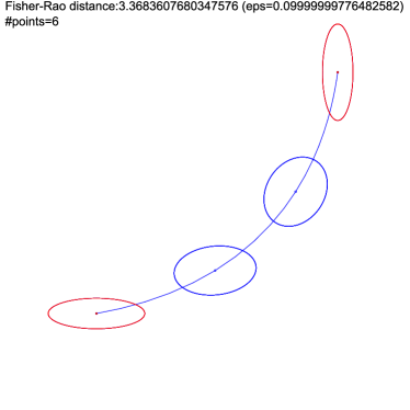
Figure 4: Some discretizations of the Fisher-Rao geodesics between two bivariate normals guaranteeing a (1+ϵ)1italic-ϵ(1+\epsilon)-approximation of the Fisher-Rao distance for ϵ{0.1,0.01,0.001,0.0001}italic-ϵ0.10.010.0010.0001\epsilon\in\{0.1,0.01,0.001,0.0001\}.

Algorithm 2. ρ~FR(N0,N1)=ApproximateRaoMVN(N0,N1,ϵ)subscript~𝜌FRsubscript𝑁0subscript𝑁1ApproximateRaoMVNsubscript𝑁0subscript𝑁1italic-ϵ\tilde{\rho}_{\mathrm{FR}}(N_{0},N_{1})=\mathrm{ApproximateRaoMVN}(N_{0},N_{1},\epsilon): l=ρCO(N0,N1)𝑙subscript𝜌COsubscript𝑁0subscript𝑁1l=\rho_{\mathrm{CO}}(N_{0},N_{1}); /* Calvo & Oller lower bound (Proposition 2.1) */ u=DJ(N0,N1)𝑢subscript𝐷𝐽subscript𝑁0subscript𝑁1u=\sqrt{D_{J}(N_{0},N_{1})}; /* Jeffreys divergence DJsubscript𝐷𝐽D_{J} (Proposition 1) */ if (ul>1+ϵ)𝑢𝑙1italic-ϵ\left(\frac{u}{l}>1+\epsilon\right) N=GeodesicMidpoint(N0,N1)𝑁GeodesicMidpointsubscript𝑁0subscript𝑁1N=\mathrm{GeodesicMidpoint}(N_{0},N_{1}); /* see Algorithm 1 for t=12𝑡12t=\frac{1}{2}. */ return ApproximateRaoMVN(N0,N,ϵ)+ApproximateRaoMVN(N,N1,ϵ)ApproximateRaoMVNsubscript𝑁0𝑁italic-ϵApproximateRaoMVN𝑁subscript𝑁1italic-ϵ\mathrm{ApproximateRaoMVN}(N_{0},N,\epsilon)+\mathrm{ApproximateRaoMVN}(N,N_{1},\epsilon); else return u;

Theorem 2.2.

We can compute a (1+ϵ)1italic-ϵ(1+\epsilon)-approximation of the Fisher-Rao distance between two multivariate normal distributions for any ϵ>0italic-ϵ0\epsilon>0.

Proof.

The proof follows from the fact that when ul1+ϵ𝑢𝑙1italic-ϵ\frac{u}{l}\leq 1+\epsilon then we have

DJ(N0,N1)(1+ϵ)ρCO(N0,N1)(1+ϵ)ρFR(N0,N1).\sqrt{D_{J}(N_{0},N_{1})}\leq(1+\epsilon)\rho_{\mathrm{CO}}(N_{0},N_{1})\leq\leq(1+\epsilon)\rho_{\mathrm{FR}}(N_{0},N_{1}).

Since we cut recursively along the geodesics γFR(N0,N1)subscript𝛾FRsubscript𝑁0subscript𝑁1\gamma_{\mathrm{FR}}(N_{0},N_{1}) into overall T+1𝑇1T+1 pieces NiTsubscript𝑁𝑖𝑇N_{\frac{i}{T}}, we have

ρ~FR(N0,N1)=i=0T1ρ~(NiT,i+1T)i=0T1(1+ϵ)ρFR((NiT,i+1T).\tilde{\rho}_{\mathrm{FR}}(N_{0},N_{1})=\sum_{i=0}^{T-1}\tilde{\rho}(N_{\frac{i}{T}},_{\frac{i+1}{T}})\leq\sum_{i=0}^{T-1}(1+\epsilon)\rho_{\mathrm{FR}}((N_{\frac{i}{T}},_{\frac{i+1}{T}}).

But γFR(N0,N1)subscript𝛾FRsubscript𝑁0subscript𝑁1\gamma_{\mathrm{FR}}(N_{0},N_{1}) is totally geodesic so that i=0T1ρFR((NiT,i+1T)=ρFR(N0,N1)\sum_{i=0}^{T-1}\rho_{\mathrm{FR}}((N_{\frac{i}{T}},_{\frac{i+1}{T}})=\rho_{\mathrm{FR}}(N_{0},N_{1}). It follows that

ρ~FR(N0,N1)(1+ϵ)ρFR(N0,N1).subscript~𝜌FRsubscript𝑁0subscript𝑁11italic-ϵsubscript𝜌FRsubscript𝑁0subscript𝑁1\tilde{\rho}_{\mathrm{FR}}(N_{0},N_{1})\leq(1+\epsilon)\rho_{\mathrm{FR}}(N_{0},N_{1}).

Instead of computing exactly the geodesic midpoint γFR(N0,N1;12)subscript𝛾FRsubscript𝑁0subscript𝑁112\gamma_{\mathrm{FR}}(N_{0},N_{1};\frac{1}{2}), we may use the matrix arithmetic-harmonic mean algorithm of [55] which convergence quadratically to the geometric matrix mean of 𝒩¯0subscript¯𝒩0{\overline{\mathcal{N}}}_{0} and 𝒩¯1subscript¯𝒩1{\overline{\mathcal{N}}}_{1} (i.e., the geodesic midpoint). The matrix AHM only requires to compute matrix inverses for calculating the matrix harmonic means (see Appendix C).

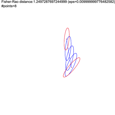
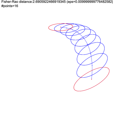
Figure 4 shows the discretization steps of the Fisher-Rao geodesic between two bivariate normal distributions for ϵ{0.1,0.01,0.001,0.0001}italic-ϵ0.10.010.0010.0001\epsilon\in\{0.1,0.01,0.001,0.0001\} with the number of control points on the geodesics and the guaranteed (1+ϵ)1italic-ϵ(1+\epsilon)-approximation of the Fisher-Rao distance. Figure 5 illustrates several examples of discretized Fisher-Rao geodesics between bivariate normal distributions obtained for ϵ=0.01italic-ϵ0.01\epsilon=0.01.

Refer to caption Refer to caption
Figure 5: Some discretizations of the Fisher-Rao geodesics between two random bivariate normals guaranteeing a (1+ϵ)1italic-ϵ(1+\epsilon)-approximation of the Fisher-Rao distance for ϵ=0.01italic-ϵ0.01\epsilon=0.01.

3 Fisher-Rao clustering

We shall consider two applications of the Fisher-Rao distance between MVNs using clustering:

The first application considers clustering weighted MVNs which is useful to simplify Gaussian Mixture Models [28, 69] (GMMs): A GMM m(x)=i=1nwipμi,Σi(x)𝑚𝑥superscriptsubscript𝑖1𝑛subscript𝑤𝑖subscript𝑝subscript𝜇𝑖subscriptΣ𝑖𝑥m(x)=\sum_{i=1}^{n}w_{i}p_{\mu_{i},\Sigma_{i}}(x) with n𝑛n components is a weighted set of n𝑛n MVNs N(μi,Σi)𝑁subscript𝜇𝑖subscriptΣ𝑖N(\mu_{i},\Sigma_{i}) and clustering this set into k𝑘k-clusters allows one to simplify the GMM m(x)𝑚𝑥m(x). For this task, we may use the k𝑘k-means clustering [53] when centroids are available in closed-form [28] (using the Kullback-Leibler divergence) or the k𝑘k-medioid clustering [48] when we choose the representative of clusters from the input otherwise (using the Fisher-Rao distance).

The second application considers the quantization of sets of MVNs which is useful to further compress a set {m1,,mn}subscript𝑚1subscript𝑚𝑛\{m_{1},\ldots,m_{n}\} of n𝑛n GMMs mi(x)=j=1niwi,jpμi,j,Σi,j(x)subscript𝑚𝑖𝑥superscriptsubscript𝑗1subscript𝑛𝑖subscript𝑤𝑖𝑗subscript𝑝subscript𝜇𝑖𝑗subscriptΣ𝑖𝑗𝑥m_{i}(x)=\sum_{j=1}^{n_{i}}w_{i,j}p_{\mu_{i,j},\Sigma_{i,j}}(x) with overall N=i=1nni𝑁superscriptsubscript𝑖1𝑛subscript𝑛𝑖N=\sum_{i=1}^{n}n_{i} MVNs N(μi,j,Σi,j)𝑁subscript𝜇𝑖𝑗subscriptΣ𝑖𝑗N(\mu_{i,j},\Sigma_{i,j}). We build a codebook of k𝑘k MVNs N(mi,Si)𝑁subscript𝑚𝑖subscript𝑆𝑖N(m_{i},S_{i}) by quantizing the N𝑁N non-weighted MVNs using the guaranteed k𝑘k-center clustering of [38] (also called k𝑘k-centers clustering [30]). Then each mixture mi(x)subscript𝑚𝑖𝑥m_{i}(x) is quantized into a mixture m~wi(x)=i=1kwi,jpmi,Si(x)subscript~𝑚subscript𝑤𝑖𝑥superscriptsubscript𝑖1𝑘subscript𝑤𝑖𝑗subscript𝑝subscript𝑚𝑖subscript𝑆𝑖𝑥\tilde{m}_{w_{i}}(x)=\sum_{i=1}^{k}w_{i,j}p_{m_{i},S_{i}}(x). The advantage of quantization is that the original set {m1,,mn}subscript𝑚1subscript𝑚𝑛\{m_{1},\ldots,m_{n}\} of GMMs is compactly represented by n𝑛n points in the (k1)𝑘1(k-1)-dimensional standard simplex Δk1subscriptΔ𝑘1\Delta_{k-1} encoding {m~1,,m~n}subscript~𝑚1subscript~𝑚𝑛\{\tilde{m}_{1},\ldots,\tilde{m}_{n}\} since they share the same components. The set {m~w:wΔk1}conditional-setsubscript~𝑚𝑤𝑤subscriptΔ𝑘1\{\tilde{m}_{w}\ :\ w\in\Delta_{k-1}\} form a mixture family in information geometry [5, 57] with a dually flat space which can be exploited algorithmically.

Notice that minimizing the objective functions of these k𝑘k-means, k𝑘k-medioid and k𝑘k-center clustering objective are NP-hard when dealing with MVNs.

3.1 Nearest neighbor queries

In order to speed up these center-based clustering, we shall find for a given MVN N(μ,Σ)𝑁𝜇ΣN(\mu,\Sigma) (a query) its closest cluster center among k𝑘k MVNs {N(mi,Si)}𝑁subscript𝑚𝑖subscript𝑆𝑖\{N(m_{i},S_{i})\} using Nearest Neighbor (NN) query search [6, 12]. There exist many data-structures for exact and approximate NN queries. For example, the vantage point (VP) tree structure is well-suited in metric spaces [76] and has also been considered for NN queries with respect to the Kullback-Leibler divergence between MVNs [58]. Although NN queries based on VP-trees still require linear time in the worst-case, they can also achieve logarithmic time in best cases. At the heart of NN search using VP-trees, we are given a query ball Ball(p,r)Ball𝑝𝑟\mathrm{Ball}(p,r) with center p𝑝p and radius r𝑟r, and we need to find potential intersections with balls Ball(v,rv)Ball𝑣subscript𝑟𝑣\mathrm{Ball}(v,r_{v}) stored at nodes v𝑣v of the VP tree. Thus when using the (fine approximation ρ~Tsubscript~𝜌𝑇\tilde{\rho}_{T}) Fisher-Rao metric distance, we need to answer predicates of whether two Fisher-Rao balls BallFR(N,r)subscriptBallFR𝑁𝑟\mathrm{Ball}_{\mathrm{FR}}(N,r) and BallFR(N,r)subscriptBallFRsuperscript𝑁superscript𝑟\mathrm{Ball}_{\mathrm{FR}}(N^{\prime},r^{\prime}) intersect or not: This can be done by determining the sign of ρFR(N,N)(r+r)subscript𝜌FR𝑁superscript𝑁𝑟superscript𝑟\rho_{\mathrm{FR}}(N,N^{\prime})-(r+r^{\prime}). When positive the balls do not intersect and when negative the balls intersect. Since we handle some approximation errors by using ρ~Tsubscript~𝜌𝑇\tilde{\rho}_{T} instead of ρFRsubscript𝜌FR\rho_{\mathrm{FR}}, but since ρ~TρFRsubscript~𝜌𝑇subscript𝜌FR\tilde{\rho}_{T}\geq\rho_{\mathrm{FR}} we need to explore both branches of a VP-tree if the balls BallFR(N,r)subscriptBallFR𝑁𝑟\mathrm{Ball}_{\mathrm{FR}}(N,r) and BallFR(N,r)subscriptBallFRsuperscript𝑁superscript𝑟\mathrm{Ball}_{\mathrm{FR}}(N^{\prime},r^{\prime}) stored at the two siblings of a node v𝑣v are such that ρ~T(N,N)r+rsubscript~𝜌𝑇𝑁superscript𝑁𝑟superscript𝑟\tilde{\rho}_{T}(N,N^{\prime})\leq r+r^{\prime}.

3.2 k𝑘k-centers clustering and miniball

For the quantization tasks, the k𝑘k-center clustering heuristic of Gonzalez [38] guarantees to find a good k𝑘k-center clustering in metric spaces with an approximation factor upper bounded by 222. We can further refine the cluster representative of each cluster by computing approximations of the smallest enclosing Fisher-Rao balls (miniballs) of clusters.

A simple Riemannian approximation technique has been reported for approximating the smallest enclosing ball of n𝑛n points {p1,,pn}subscript𝑝1subscript𝑝𝑛\{p_{1},\ldots,p_{n}\} on a Riemannian manifold (M,g)𝑀𝑔(M,g) with geodesic distance ρg(p,p)subscript𝜌𝑔𝑝superscript𝑝\rho_{g}(p,p^{\prime}) and geodesics γg(p,p;t)subscript𝛾𝑔𝑝superscript𝑝𝑡\gamma_{g}(p,p^{\prime};t) in [7]:

Miniball({p1,,pn},ρg,Tsubscript𝑝1subscript𝑝𝑛subscript𝜌𝑔𝑇\{p_{1},\ldots,p_{n}\},\rho_{g},T):

  • Let c1p1subscript𝑐1subscript𝑝1c_{1}\leftarrow p_{1}

  • For t=1𝑡1t=1 to T𝑇T

    • Compute the index of the point which is farthest to current circumcenter ctsubscript𝑐𝑡c_{t}:

      ft=argmaxi{1,,n}ρg(ct,pi)subscript𝑓𝑡subscript𝑖1𝑛subscript𝜌𝑔subscript𝑐𝑡subscript𝑝𝑖f_{t}=\arg\max_{i\in\{1,\ldots,n\}}\rho_{g}(c_{t},p_{i})
    • Update the circumcenter by walking along the geodesic linking ctsubscript𝑐𝑡c_{t} to pftsubscript𝑝subscript𝑓𝑡p_{f_{t}}:

      ct+1=γg(ct,pft;1t+1)subscript𝑐𝑡1subscript𝛾𝑔subscript𝑐𝑡subscript𝑝subscript𝑓𝑡1𝑡1c_{t+1}=\gamma_{g}\left(c_{t},p_{f_{t}};\frac{1}{t+1}\right)

      Recall that geodesics are parameterized by normalized arc length so that ρg(ct,ct+1)=1t+1ρg(ct,pft)subscript𝜌𝑔subscript𝑐𝑡subscript𝑐𝑡11𝑡1subscript𝜌𝑔subscript𝑐𝑡subscript𝑝subscript𝑓𝑡\rho_{g}(c_{t},c_{t+1})=\frac{1}{t+1}\rho_{g}(c_{t},p_{f_{t}}).

  • Return cTsubscript𝑐𝑇c_{T}

Conditions of convergence are analyzed in [7]: For example, it always converge for Cartan-Hadamard manifolds (complete simply connected NPC manifolds like the SPD cone).

The Fisher-Rao distance ρFR(NΣ(μ0),NΣ(μ1))subscript𝜌FRsubscript𝑁Σsubscript𝜇0subscript𝑁Σsubscript𝜇1\rho_{\mathrm{FR}}(N_{\Sigma}(\mu_{0}),N_{\Sigma}(\mu_{1})) between two MVNs with same covariance matrix ΣΣ\Sigma is

ρFR(NΣ(μ0),NΣ(μ1))=2arccosh(1+14ΔΣ2(μ0,μ1)),subscript𝜌FRsubscript𝑁Σsubscript𝜇0subscript𝑁Σsubscript𝜇12arccosh114superscriptsubscriptΔΣ2subscript𝜇0subscript𝜇1\rho_{\mathrm{FR}}(N_{\Sigma}(\mu_{0}),N_{\Sigma}(\mu_{1}))=\sqrt{2}\,\mathrm{arccosh}\left(1+\frac{1}{4}\Delta_{\Sigma}^{2}(\mu_{0},\mu_{1})\right),

where ΔΣ(μ0,μ1)=(μ0μ1)Σ1(μ20μ1)subscriptΔΣsubscript𝜇0subscript𝜇1superscriptsubscript𝜇0subscript𝜇1topsuperscriptΣ1subscript𝜇20subscript𝜇1\Delta_{\Sigma}(\mu_{0},\mu_{1})=\sqrt{(\mu_{0}-\mu_{1})^{\top}\Sigma^{-1}(\mu_{2}0-\mu_{1})} is the Mahalanobis distance. Therefore when all MVNs belong to the non-totally flat submanifold 𝒩Σ={N(μ,Σ):μd}subscript𝒩Σconditional-set𝑁𝜇Σ𝜇superscript𝑑\mathcal{N}_{\Sigma}=\{N(\mu,\Sigma)\ :\ \mu\in\mathbb{R}^{d}\}, the smallest enclosing ball amounts to an Euclidean smallest enclosing ball [75] since in that case ρFRsubscript𝜌FR\rho_{\mathrm{FR}} is an increasing function of the Mahalanobis distance.

Since the computations of ρ~Tsubscript~𝜌𝑇\tilde{\rho}_{T} approximating ρFRsubscript𝜌FR\rho_{\mathrm{FR}} is costly, the following section shall consider a new fast metric distance on 𝒩𝒩\mathcal{N} which further relates to the Fisher-Rao distance.

4 Pullback Hilbert cone distance

Let us define dissimilarities and paths on 𝒩(d)𝒩𝑑\mathcal{N}(d) from dissimilarities and geodesics on 𝒫(d+1)=𝒩0(d)𝒫𝑑1subscript𝒩0𝑑\mathcal{P}(d+1)=\mathcal{N}_{0}(d) by considering the following family of diffeomorphic embeddings fa:𝒩(d)𝒫(d+1):subscript𝑓𝑎𝒩𝑑𝒫𝑑1f_{a}:\mathcal{N}(d)\rightarrow\mathcal{P}(d+1) for a>0𝑎subscriptabsent0a\in\mathbb{R}_{>0} proposed in [20]:

fa(N(μ,Σ)):=[Σ+aμμaμaμa]𝒫(d+1).assignsubscript𝑓𝑎𝑁𝜇Σdelimited-[]Σ𝑎𝜇superscript𝜇top𝑎𝜇𝑎superscript𝜇top𝑎𝒫𝑑1f_{a}(N(\mu,\Sigma)){:=}{\left[\begin{array}[]{ll}\Sigma+a\mu\mu^{\top}&a\mu\cr a\mu^{\top}&a\end{array}\right]}\in\mathcal{P}(d+1). (20)

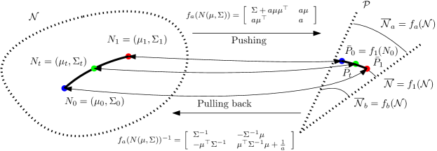
Let 𝒩¯a(d)={fa(N):N𝒩(d)}𝒫(d+1)subscript¯𝒩𝑎𝑑conditional-setsubscript𝑓𝑎𝑁𝑁𝒩𝑑𝒫𝑑1\overline{\mathcal{N}}_{a}(d)=\{f_{a}(N)\ :\ N\in\mathcal{N}(d)\}\subset\mathcal{P}(d+1) denote the embedded Gaussian submanifold in 𝒫(d+1)𝒫𝑑1\mathcal{P}(d+1) of codimension 111 that is obtained by pushing the normals to SPD matrices (Figure 6). We let fainv:𝒩¯a(d)𝒩(d):superscriptsubscript𝑓𝑎invsubscript¯𝒩𝑎𝑑𝒩𝑑f_{a}^{\mathrm{inv}}:\overline{\mathcal{N}}_{a}(d)\rightarrow\mathcal{N}(d) denote the functional inverse so that fafainv=id𝒩subscript𝑓𝑎superscriptsubscript𝑓𝑎inv𝑖subscript𝑑𝒩f_{a}\circ f_{a}^{\mathrm{inv}}=id_{\mathcal{N}} is the identity function id𝒩:𝒩𝒩:subscriptid𝒩𝒩𝒩\mathrm{id}_{\mathcal{N}}:\mathcal{N}\rightarrow\mathcal{N}. Function fainvsuperscriptsubscript𝑓𝑎invf_{a}^{\mathrm{inv}} pulls back the SPD matrices to the normal distributions (Figure 6). The notation invinv\mathrm{inv} in fainvsuperscriptsubscript𝑓𝑎invf_{a}^{\mathrm{inv}} is chosen to avoid confusion with the matrix inverse fa(N(μ,Σ))1subscript𝑓𝑎superscript𝑁𝜇Σ1f_{a}(N(\mu,\Sigma))^{-1}:

fa(N(μ,Σ))1=[Σ1Σ1μμΣ1μΣ1μ+1a].subscript𝑓𝑎superscript𝑁𝜇Σ1delimited-[]superscriptΣ1superscriptΣ1𝜇superscript𝜇topsuperscriptΣ1superscript𝜇topsuperscriptΣ1𝜇1𝑎f_{a}(N(\mu,\Sigma))^{-1}={\left[\begin{array}[]{ll}\Sigma^{-1}&-\Sigma^{-1}\mu\cr-\mu^{\top}\Sigma^{-1}&\mu^{\top}\Sigma^{-1}\mu+\frac{1}{a}\end{array}\right]}.
Refer to caption
Figure 6: Pushing the d𝑑d-dimensional normals 𝒩𝒩\mathcal{N} to a submanifold 𝒩¯¯𝒩\overline{\mathcal{N}} of the (d+1)×(d+1)𝑑1𝑑1(d+1)\times(d+1)-dimensional SPD cone via a diffeomorphic embedding f𝑓f, and pulling back a geodesic/curve on the SPD cone to the normal manifold with f1superscript𝑓1f^{-1}.

The open SPD cone 𝒫(d+1)𝒫𝑑1\mathcal{P}(d+1) can thus be foliated by the family of submanifolds 𝒩¯asubscript¯𝒩𝑎\overline{\mathcal{N}}_{a} [20]: 𝒫(d+1)={a×𝒩¯a:a>0}𝒫𝑑1conditional-set𝑎subscript¯𝒩𝑎𝑎subscriptabsent0\mathcal{P}(d+1)=\left\{a\times\overline{\mathcal{N}}_{a}\ :\ a\in\mathbb{R}_{>0}\right\}. We let f=f1𝑓subscript𝑓1f=f_{1} and finv=f1invsuperscript𝑓invsuperscriptsubscript𝑓1invf^{\mathrm{inv}}=f_{1}^{\mathrm{inv}}, and 𝒩¯=𝒩¯1¯𝒩subscript¯𝒩1\overline{\mathcal{N}}=\overline{\mathcal{N}}_{1}.

Calvo and Oller [20] proved that (𝒩(d),gFisher)𝒩𝑑subscript𝑔Fisher(\mathcal{N}(d),g_{\mathrm{Fisher}}) is isometrically embedded into (𝒫(d+1),12gtrace)𝒫𝑑112subscript𝑔trace(\mathcal{P}(d+1),\frac{1}{2}g_{\mathrm{trace}}) but that 𝒩¯¯𝒩\overline{\mathcal{N}} is not totally geodesic. Thus we have

ρCO(N0,N1)subscript𝜌COsubscript𝑁0subscript𝑁1\displaystyle\rho_{\mathrm{CO}}(N_{0},N_{1}) =\displaystyle= ρFR(N(0,f(N0)),N(0,f(N1))),subscript𝜌FR𝑁0𝑓subscript𝑁0𝑁0𝑓subscript𝑁1\displaystyle\rho_{\mathrm{FR}}(N(0,f(N_{0})),N(0,f(N_{1}))),
=\displaystyle= ρ𝒫(𝒩¯0,𝒩¯1)ρFR(N0,N1),subscript𝜌𝒫subscript¯𝒩0subscript¯𝒩1subscript𝜌FRsubscript𝑁0subscript𝑁1\displaystyle\rho_{\mathcal{P}}({\overline{\mathcal{N}}}_{0},{\overline{\mathcal{N}}}_{1})\geq\rho_{\mathrm{FR}}(N_{0},N_{1}),

where 𝒩¯i=f(Ni)subscript¯𝒩𝑖𝑓subscript𝑁𝑖{\overline{\mathcal{N}}}_{i}=f(N_{i}). See Eq. 5. It follows that we get a series of lower bound for ρFR(N0,N1)subscript𝜌FRsubscript𝑁0subscript𝑁1\rho_{\mathrm{FR}}(N_{0},N_{1}):

ρCO,T(N0,N1)=i=0T1ρ𝒫(NiT,Ni+1T),subscript𝜌CO𝑇subscript𝑁0subscript𝑁1superscriptsubscript𝑖0𝑇1subscript𝜌𝒫subscript𝑁𝑖𝑇subscript𝑁𝑖1𝑇\rho_{\mathrm{CO},T}(N_{0},N_{1})=\sum_{i=0}^{T-1}\rho_{\mathcal{P}}\left(N_{\frac{i}{T}},N_{\frac{i+1}{T}}\right),

such that for all T𝑇T, ρ~TρFRρCO,Tsubscript~𝜌𝑇subscript𝜌FRsubscript𝜌CO𝑇\tilde{\rho}_{T}\geq\rho_{\mathrm{FR}}\geq\rho_{\mathrm{CO},T}.

We can also approximate the smallest enclosing Fisher-Rao ball of {N(μi,Σi)}𝑁subscript𝜇𝑖subscriptΣ𝑖\{N(\mu_{i},\Sigma_{i})\} on 𝒩(d)𝒩𝑑\mathcal{N}(d) by embedding the normals into 𝒩¯¯𝒩\overline{\mathcal{N}} as {P¯i=f(N(μi,Σi))}subscript¯𝑃𝑖𝑓𝑁subscript𝜇𝑖subscriptΣ𝑖\{{\bar{P}}_{i}=f(N(\mu_{i},\Sigma_{i}))\}. We then apply the above iterative smallest enclosing ball approximation Miniball [7] to get C~T𝒫(d+1)subscript~𝐶𝑇𝒫𝑑1\tilde{C}_{T}\in\mathcal{P}(d+1) after T𝑇T iterations. Then we project orthogonally with respect to the trace metric C~Tsubscript~𝐶𝑇\tilde{C}_{T} onto 𝒩¯¯𝒩\overline{\mathcal{N}} as C¯T=proj𝒩¯(C~T)subscript¯𝐶𝑇subscriptproj¯𝒩subscript~𝐶𝑇\bar{C}_{T}=\mathrm{proj}_{{\overline{\mathcal{N}}}}(\tilde{C}_{T}) and maps back to the Gaussian manifold using finvsuperscript𝑓invf^{\mathrm{inv}} to get the approximate normal circumcenter.

The following proposition describes the orthogonal projection operation P¯=proj𝒩¯(P)subscript¯𝑃perpendicular-tosubscriptproj¯𝒩𝑃{\bar{P}}_{\perp}=\mathrm{proj}_{{\overline{\mathcal{N}}}}(P) of P=[Pi,j]𝒫(d+1)𝑃delimited-[]subscript𝑃𝑖𝑗𝒫𝑑1P=[P_{i,j}]\in\mathcal{P}(d+1) onto 𝒩¯¯𝒩{\overline{\mathcal{N}}} based on the analysis reported in the Appendix of [20] (page 239):

Proposition 4.1.

Let β=Pd+1,d+1𝛽subscript𝑃𝑑1𝑑1\beta=P_{d+1,d+1} and write P=[Σ+βμμβμβμβ]𝑃delimited-[]Σ𝛽𝜇superscript𝜇top𝛽𝜇𝛽superscript𝜇top𝛽P={\left[\begin{array}[]{ll}\Sigma+\beta\mu\mu^{\top}&\beta\mu\cr\beta\mu^{\top}&\beta\end{array}\right]}. Then the orthogonal projection at P𝒫𝑃𝒫P\in\mathcal{P} onto 𝒩¯¯𝒩{\overline{\mathcal{N}}} is:

P¯:=proj𝒩¯(P)=[Σ+μμμμ1],assignsubscript¯𝑃perpendicular-tosubscriptproj¯𝒩𝑃delimited-[]Σ𝜇superscript𝜇topsuperscript𝜇top𝜇1{\bar{P}}_{\perp}:=\mathrm{proj}_{{\overline{\mathcal{N}}}}(P)={\left[\begin{array}[]{ll}\Sigma+\mu\mu^{\top}&\mu^{\top}\cr\mu&1\end{array}\right]}, (21)

and the SPD trace distance between P𝑃P and P¯subscript¯𝑃perpendicular-to{\bar{P}}_{\perp} is

ρ𝒫(P,P¯)=|logβ|.subscript𝜌𝒫𝑃subscript¯𝑃perpendicular-to𝛽\rho_{\mathcal{P}}(P,{\bar{P}}_{\perp})=|\log\beta|. (22)

Consider pulling back SPD cone dissimilarities and geodesics of 𝒫(d+1)𝒫𝑑1\mathcal{P}(d+1) onto 𝒩(d)𝒩𝑑\mathcal{N}(d) as follows:

Definition 4.2 (Pullback dissimilarities).

A dissimilarity D(N0,N1)𝐷subscript𝑁0subscript𝑁1D(N_{0},N_{1}) (not necessarily be a metric distance nor a smooth divergence) on 𝒩(d)𝒩𝑑\mathcal{N}(d) (with N0:=N(μ0,Σ0)assignsubscript𝑁0𝑁subscript𝜇0subscriptΣ0N_{0}{:=}N(\mu_{0},\Sigma_{0}) and N1:=N(μ1,Σ1)assignsubscript𝑁1𝑁subscript𝜇1subscriptΣ1N_{1}{:=}N(\mu_{1},\Sigma_{1})) can be obtained from any dissimilarity DSPD(,)subscript𝐷SPDD_{\mathrm{SPD}}(\cdot,\cdot) on the SPD cone by pulling back the SPD matrix cone dissimilarity using f𝑓f:

D(N0,N1):=DSPD(f(N0),f(N1)).assign𝐷subscript𝑁0subscript𝑁1subscript𝐷SPD𝑓subscript𝑁0𝑓subscript𝑁1D(N_{0},N_{1}){:=}D_{\mathrm{SPD}}(f(N_{0}),f(N_{1})). (23)

Similarly, we pullback cone geodesics onto 𝒩𝒩\mathcal{N}:

Definition 4.3 (Pullback curves).

A path cγ(N0,N1;t)subscript𝑐𝛾subscript𝑁0subscript𝑁1𝑡c_{\gamma}(N_{0},N_{1};t) joining N0=cγ(N0,N1;0)subscript𝑁0subscript𝑐𝛾subscript𝑁0subscript𝑁10N_{0}=c_{\gamma}(N_{0},N_{1};0) and N1=cγ(N0,N1;1)subscript𝑁1subscript𝑐𝛾subscript𝑁0subscript𝑁11N_{1}=c_{\gamma}(N_{0},N_{1};1) can be defined by the pullback of any geodesic γ(f(N0),f(N1);t)𝛾𝑓subscript𝑁0𝑓subscript𝑁1𝑡\gamma(f(N_{0}),f(N_{1});t) on the SPD cone:

cγ(N0,N1;t):=finv(γ(f(N0),f(N1);t)).assignsubscript𝑐𝛾subscript𝑁0subscript𝑁1𝑡superscript𝑓inv𝛾𝑓subscript𝑁0𝑓subscript𝑁1𝑡c_{\gamma}(N_{0},N_{1};t){:=}f^{\mathrm{inv}}(\gamma(f(N_{0}),f(N_{1});t)). (24)

Hence, we can leverage the rich literature on dissimilarities and geodesics on the SPD cone (e.g., [41, 23, 68, 8, 24]). Note that the Riemannian SPD trace metric geodesic is also the geodesic for Finslerian distances ρh(P0,P1):=Log(P012P1P012)hassignsubscript𝜌subscript𝑃0subscript𝑃1subscriptnormLogsuperscriptsubscript𝑃012subscript𝑃1superscriptsubscript𝑃012\rho_{h}(P_{0},P_{1}){:=}\left\|{\mathrm{Log}}\left(P_{0}^{-\frac{1}{2}}\,P_{1}\,P_{0}^{-\frac{1}{2}}\right)\right\|_{h} where hh is a totally symmetric gauge function (i.e., h(x1,,xn)=h(σ(x1,,xn))subscript𝑥1subscript𝑥𝑛𝜎subscript𝑥1subscript𝑥𝑛h(x_{1},\ldots,x_{n})=h(\sigma(x_{1},\ldots,x_{n})) for any permutation σ𝜎\sigma)) and Ph:=h(λ1(P),,λd(P))assignsubscriptnorm𝑃subscript𝜆1𝑃subscript𝜆𝑑𝑃\|P\|_{h}{:=}h(\lambda_{1}(P),\ldots,\lambda_{d}(P)). When h(x)=hp(x)=xp=(i=1dxip)1p𝑥subscript𝑝𝑥subscriptnorm𝑥𝑝superscriptsuperscriptsubscript𝑖1𝑑superscriptsubscript𝑥𝑖𝑝1𝑝h(x)=h_{p}(x)=\|x\|_{p}=\left(\sum_{i=1}^{d}x_{i}^{p}\right)^{\frac{1}{p}} is the p𝑝p-norm for 1p<1𝑝1\leq p<\infty, we get the Schatten matrix p𝑝p-norms [13].

Refer to caption


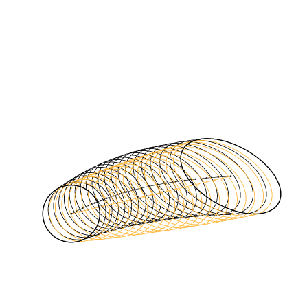
Figure 7: Comparing the pullback Hilbert geodesic (orange, coinciding with the mixture geodesic) with the exact Fisher-Rao geodesic displayed in black.

The Hilbert projective distance also called Birkhoff projective distance [42, 15, 24] on the SPD cone Sym+(d,)subscriptSym𝑑\mathrm{Sym}_{+}(d,\mathbb{R}) is defined by

ρHilbert(P0,P1)subscript𝜌Hilbertsubscript𝑃0subscript𝑃1\displaystyle\rho_{\mathrm{Hilbert}}(P_{0},P_{1}) =\displaystyle= log(λmax(P012P1P012)λmin(P012P1P012)),subscript𝜆maxsuperscriptsubscript𝑃012subscript𝑃1superscriptsubscript𝑃012subscript𝜆minsuperscriptsubscript𝑃012subscript𝑃1superscriptsubscript𝑃012\displaystyle\log\left(\frac{\lambda_{{\mathrm{max}}}(P_{0}^{-\frac{1}{2}}P_{1}P_{0}^{-\frac{1}{2}})}{\lambda_{{\mathrm{min}}}(P_{0}^{-\frac{1}{2}}P_{1}P_{0}^{-\frac{1}{2}})}\right),
=\displaystyle= log(λmax(P01P1)λmin(P01P1)).subscript𝜆maxsuperscriptsubscript𝑃01subscript𝑃1subscript𝜆minsuperscriptsubscript𝑃01subscript𝑃1\displaystyle\log\left(\frac{\lambda_{{\mathrm{max}}}(P_{0}^{-1}P_{1})}{\lambda_{{\mathrm{min}}}(P_{0}^{-1}P_{1})}\right).

It is a projective distance (or quasi-metric distance) because it is symmetric and satisfies the triangular inequality but we have ρHilbert(P0,P1)=0subscript𝜌Hilbertsubscript𝑃0subscript𝑃10\rho_{\mathrm{Hilbert}}(P_{0},P_{1})=0 if and only if P0=λP1subscript𝑃0𝜆subscript𝑃1P_{0}=\lambda P_{1} for some λ>0𝜆0\lambda>0. It was proven in [50] (Theorem 4.1) that any projective distance with strict contraction ratio under linear mapping is necessarily a scalar function of the Hilbert’s projective metric, and that the Hilbert projective distance has the lowest possible contraction ratio.

However, the pullback Hilbert distance on 𝒩𝒩\mathcal{N}, ρHilbert(N0,N1):=ρHilbert(f(N0),f(N1))assignsubscript𝜌Hilbertsubscript𝑁0subscript𝑁1subscript𝜌Hilbert𝑓subscript𝑁0𝑓subscript𝑁1\rho_{\mathrm{Hilbert}}(N_{0},N_{1}):=\rho_{\mathrm{Hilbert}}(f(N_{0}),f(N_{1})), is a proper metric distance on 𝒩¯¯𝒩\overline{\mathcal{N}} since f(N0)=f(N1)𝑓subscript𝑁0𝑓subscript𝑁1f(N_{0})=f(N_{1}) if and only if λ=1𝜆1\lambda=1 because the array element at last row and last column [f(N0)]d+1,d+1=[f(N1)]d+1,d+1=1subscriptdelimited-[]𝑓subscript𝑁0𝑑1𝑑1subscriptdelimited-[]𝑓subscript𝑁1𝑑1𝑑11[f(N_{0})]_{d+1,d+1}=[f(N_{1})]_{d+1,d+1}=1 is identical. Thus f(N0)=λf(N1)𝑓subscript𝑁0𝜆𝑓subscript𝑁1f(N_{0})=\lambda f(N_{1}) for λ=1𝜆1\lambda=1. The pullback Hilbert cone distance only requires to calculate the extreme eigenvalues of the matrix product f(N0)1f(N1)𝑓superscriptsubscript𝑁01𝑓subscript𝑁1f(N_{0})^{-1}f(N_{1}). Thus we can bypass a costly SVD and compute approximately these extreme eigenvalues using the power method [72] (Appendix D).

The geodesic in the Hilbert SPD cone are straight lines [59] parameterized as follows:

γHilbert(P0,P1;t):=(βαtαβtβα)P0+(βtαtβα)P1,assignsubscript𝛾Hilbertsubscript𝑃0subscript𝑃1𝑡𝛽superscript𝛼𝑡𝛼superscript𝛽𝑡𝛽𝛼subscript𝑃0superscript𝛽𝑡superscript𝛼𝑡𝛽𝛼subscript𝑃1\gamma_{\mathrm{Hilbert}}(P_{0},P_{1};t):=\left(\frac{\beta\alpha^{t}-\alpha\beta^{t}}{\beta-\alpha}\right)P_{0}+\left(\frac{\beta^{t}-\alpha^{t}}{\beta-\alpha}\right)P_{1},

where α=λmin(P11P0)𝛼subscript𝜆minsuperscriptsubscript𝑃11subscript𝑃0\alpha=\lambda_{\mathrm{min}}(P_{1}^{-1}P_{0}) and β=λmax(P11P0)𝛽subscript𝜆maxsuperscriptsubscript𝑃11subscript𝑃0\beta=\lambda_{\mathrm{max}}(P_{1}^{-1}P_{0}). Figure 7 compares the pullback Hilbert geodesic curve with the Fisher-Rao geodesic.

A pregeodesic is a geodesic which may be arbitrarily reparameterized by another parameter u=r(t)𝑢𝑟𝑡u=r(t) for some smooth function r𝑟r. That is, a pregeodesic is not necessarily parameterized by arc length. Let us notice that the weighted arithmetic mean LERP(P0,P1;u)=(1u)P0+uP1LERPsubscript𝑃0subscript𝑃1𝑢1𝑢subscript𝑃0𝑢subscript𝑃1\mathrm{LERP}(P_{0},P_{1};u)=(1-u)P_{0}+uP_{1} is a pregeodesic of γHilbert(P0,P1;t)subscript𝛾Hilbertsubscript𝑃0subscript𝑃1𝑡\gamma_{\mathrm{Hilbert}}(P_{0},P_{1};t). Although Hilbert SPD space is not a Riemannian space, it enjoys non-positive curvature properties according to various definitions of curvatures [2, 47].

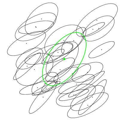
We can adapt the approximation of the minimum enclosing Hilbert ball by replacing ρFRsubscript𝜌FR\rho_{\mathrm{FR}} by ρHilbertsubscript𝜌Hilbert\rho_{\mathrm{Hilbert}} and cutting metric geodesic γHilbertsubscript𝛾Hilbert\gamma_{\mathrm{Hilbert}} instead of geodesics γFR𝒩superscriptsubscript𝛾FR𝒩\gamma_{\mathrm{FR}}^{\mathcal{N}} (see Figure 8).

Refer to caption

Figure 8: Approximating the Hilbert smallest enclosing ball of a set of bivariate normal distributions. The approximated minimax center is shown in green.

First, the diffeomorphic embedding f𝑓f exhibits several interesting features:

Proposition 4.4.

The Jeffreys divergence between pμ1,Σ1subscript𝑝subscript𝜇1subscriptΣ1p_{\mu_{1},\Sigma_{1}} and pμ2,Σ2subscript𝑝subscript𝜇2subscriptΣ2p_{\mu_{2},\Sigma_{2}} amounts to the Jeffreys divergence between qP¯1=p0,f(μ1,Σ1)subscript𝑞subscript¯𝑃1subscript𝑝0𝑓subscript𝜇1subscriptΣ1q_{\bar{P}_{1}}=p_{0,f(\mu_{1},\Sigma_{1})} and qP¯2=p0,f(μ2,Σ2)subscript𝑞subscript¯𝑃2subscript𝑝0𝑓subscript𝜇2subscriptΣ2q_{\bar{P}_{2}}=p_{0,f(\mu_{2},\Sigma_{2})} where P¯i=f(μi,Σi)subscript¯𝑃𝑖𝑓subscript𝜇𝑖subscriptΣ𝑖\bar{P}_{i}=f(\mu_{i},\Sigma_{i}): DJ(pμ1,Σ1,pμ2,Σ2)=DJ(qP¯1,qP¯2)subscript𝐷𝐽subscript𝑝subscript𝜇1subscriptΣ1subscript𝑝subscript𝜇2subscriptΣ2subscript𝐷𝐽subscript𝑞subscript¯𝑃1subscript𝑞subscript¯𝑃2D_{J}(p_{\mu_{1},\Sigma_{1}},p_{\mu_{2},\Sigma_{2}})=D_{J}(q_{\bar{P}_{1}},q_{\bar{P}_{2}}).

Proof.

Since DJ(p,q)=DKL(p,q)+DKL(q,p)subscript𝐷𝐽𝑝𝑞subscript𝐷KL𝑝𝑞subscript𝐷KL𝑞𝑝D_{J}(p,q)=D_{\mathrm{KL}}(p,q)+D_{\mathrm{KL}}(q,p), we shall prove that DKL(pμ1,Σ1,pμ2,Σ2)=DKL(qP¯1,qP¯2)subscript𝐷KLsubscript𝑝subscript𝜇1subscriptΣ1subscript𝑝subscript𝜇2subscriptΣ2subscript𝐷KLsubscript𝑞subscript¯𝑃1subscript𝑞subscript¯𝑃2D_{\mathrm{KL}}(p_{\mu_{1},\Sigma_{1}},p_{\mu_{2},\Sigma_{2}})=D_{\mathrm{KL}}(q_{\bar{P}_{1}},q_{\bar{P}_{2}}). The KLD between two centered (d+1)𝑑1(d+1)-variate normals qP1=p0,P1subscript𝑞subscript𝑃1subscript𝑝0subscript𝑃1q_{P_{1}}=p_{0,P_{1}} and qP2=p0,P2subscript𝑞subscript𝑃2subscript𝑝0subscript𝑃2q_{P_{2}}=p_{0,P_{2}} is

DKL(qP1,qP2)=12(tr(P21P1)d1+log|P2||P1|).subscript𝐷KLsubscript𝑞subscript𝑃1subscript𝑞subscript𝑃212trsuperscriptsubscript𝑃21subscript𝑃1𝑑1subscript𝑃2subscript𝑃1D_{\mathrm{KL}}(q_{P_{1}},q_{P_{2}})=\frac{1}{2}\left(\mathrm{tr}(P_{2}^{-1}P_{1})-d-1+\log\frac{|P_{2}|}{|P_{1}|}\right).

This divergence can be interpreted as the matrix version of the Itakura-Saito divergence [28]. It is a matrix spectral distance since we can write DKL(qP1,qP2)=(hKLλsp)(Σ21Σ1)subscript𝐷KLsubscript𝑞subscript𝑃1subscript𝑞subscript𝑃2subscriptKLsuperscript𝜆spsuperscriptsubscriptΣ21subscriptΣ1D_{\mathrm{KL}}(q_{P_{1}},q_{P_{2}})=(h_{\mathrm{KL}}\circ\lambda^{\mathrm{sp}})(\Sigma_{2}^{-1}\Sigma_{1}), where λsp(S)=(λ1(S),,λd(S))superscript𝜆sp𝑆subscript𝜆1𝑆subscript𝜆𝑑𝑆\lambda^{\mathrm{sp}}(S)=(\lambda_{1}(S),\ldots,\lambda_{d}(S)) and hKL(u1,,ud)=12(ui1logui)subscriptKLsubscript𝑢1subscript𝑢𝑑12subscript𝑢𝑖1subscript𝑢𝑖h_{\mathrm{KL}}(u_{1},\ldots,u_{d})=\frac{1}{2}\left(u_{i}-1-\log u_{i}\right) (a gauge function). Similarly, the Jeffreys divergence between two centered MVNs is a matrix spectral distance with gauge function hJ(u)=i=1d(ui1ui)2subscript𝐽𝑢superscriptsubscript𝑖1𝑑superscriptsubscript𝑢𝑖1subscript𝑢𝑖2h_{J}(u)=\sum_{i=1}^{d}\left(\sqrt{u_{i}}-\frac{1}{\sqrt{u_{i}}}\right)^{2}.

The SPD cone equipped with 1212\frac{1}{2} of the trace metric can be interpreted as Fisher-Rao centered normal manifolds (isometry): μ,(𝒩μ,g𝒩μFisher)(𝒫,12gtrace)for-all𝜇subscript𝒩𝜇subscriptsuperscript𝑔Fishersubscript𝒩𝜇𝒫12superscript𝑔trace\forall\mu,(\mathcal{N}_{\mu},g^{\mathrm{Fisher}}_{\mathcal{N}_{\mu}})\cong(\mathcal{P},\frac{1}{2}g^{\mathrm{trace}}).

Since the determinant of a block matrix is det([ABCD])=det(ABD1C),detdelimited-[]𝐴𝐵𝐶𝐷det𝐴𝐵superscript𝐷1𝐶\mathrm{det}\left({\left[\begin{array}[]{ll}A&B\cr C&D\end{array}\right]}\right)=\mathrm{det}\left(A-BD^{-1}C\right), we get with D=1𝐷1D=1: det(f(μ,Σ))=det(Σ+μμμμ)=det(Σ)det𝑓𝜇ΣdetΣ𝜇superscript𝜇top𝜇superscript𝜇topdetΣ\mathrm{det}(f(\mu,\Sigma))=\mathrm{det}(\Sigma+\mu\mu^{\top}-\mu\mu^{\top})=\mathrm{det}(\Sigma).

Let P¯1=f(μ1,Σ1)subscript¯𝑃1𝑓subscript𝜇1subscriptΣ1\bar{P}_{1}=f(\mu_{1},\Sigma_{1}) and P¯2=f(μ2,Σ2)subscript¯𝑃2𝑓subscript𝜇2subscriptΣ2\bar{P}_{2}=f(\mu_{2},\Sigma_{2}). Checking DKL[pμ1,Σ1:pμ2,Σ2]=DKL[qP¯1:qP¯2]D_{\mathrm{KL}}[p_{\mu_{1},\Sigma_{1}}:p_{\mu_{2},\Sigma_{2}}]=D_{\mathrm{KL}}[q_{\bar{P}_{1}}:q_{\bar{P}_{2}}] where qP¯=p0,P¯subscript𝑞¯𝑃subscript𝑝0¯𝑃q_{{\bar{P}}}=p_{0,{\bar{P}}} amounts to verify that tr(P¯21P¯1)=1+tr(Σ21Σ1+ΔμΣ21Δμ)trsuperscriptsubscript¯𝑃21subscript¯𝑃11trsuperscriptsubscriptΣ21subscriptΣ1superscriptsubscriptΔ𝜇topsuperscriptsubscriptΣ21subscriptΔ𝜇\mathrm{tr}(\bar{P}_{2}^{-1}\bar{P}_{1})=1+\mathrm{tr}(\Sigma_{2}^{-1}\Sigma_{1}+\Delta_{\mu}^{\top}\Sigma_{2}^{-1}\Delta_{\mu}). Indeed, using the inverse matrix

f(μ,Σ)1=[Σ1Σ1μμΣ11+μΣ1μ],𝑓superscript𝜇Σ1delimited-[]superscriptΣ1superscriptΣ1𝜇superscript𝜇topsuperscriptΣ11superscript𝜇topsuperscriptΣ1𝜇f(\mu,\Sigma)^{-1}={\left[\begin{array}[]{ll}\Sigma^{-1}&-\Sigma^{-1}\mu\cr-\mu^{\top}\Sigma^{-1}&1+\mu^{\top}\Sigma^{-1}\mu\end{array}\right]},

we have tr(P¯21P¯1)=tr([Σ21Σ21μ2μ2Σ211+μ2Σ21μ2][Σ1+μ1μ1μ1μ11])=1+tr(Σ21Σ1+ΔμΣ21Δμ)trsuperscriptsubscript¯𝑃21subscript¯𝑃1trdelimited-[]subscriptsuperscriptΣ12subscriptsuperscriptΣ12subscript𝜇2superscriptsubscript𝜇2topsuperscriptsubscriptΣ211superscriptsubscript𝜇2topsubscriptsuperscriptΣ12subscript𝜇2delimited-[]subscriptΣ1subscript𝜇1superscriptsubscript𝜇1topsubscript𝜇1superscriptsubscript𝜇1top11trsuperscriptsubscriptΣ21subscriptΣ1superscriptsubscriptΔ𝜇topsuperscriptsubscriptΣ21subscriptΔ𝜇\mathrm{tr}(\bar{P}_{2}^{-1}\bar{P}_{1})=\mathrm{tr}\left({\left[\begin{array}[]{ll}\Sigma^{-1}_{2}&-\Sigma^{-1}_{2}\mu_{2}\cr-\mu_{2}^{\top}\Sigma_{2}^{-1}&1+\mu_{2}^{\top}\Sigma^{-1}_{2}\mu_{2}\end{array}\right]}\ {\left[\begin{array}[]{ll}\Sigma_{1}+\mu_{1}\mu_{1}^{\top}&\mu_{1}\cr\mu_{1}^{\top}&1\end{array}\right]}\right)=1+\mathrm{tr}(\Sigma_{2}^{-1}\Sigma_{1}+\Delta_{\mu}^{\top}\Sigma_{2}^{-1}\Delta_{\mu}). Thus even if the dimension of the sample spaces of pμ,Σsubscript𝑝𝜇Σp_{\mu,\Sigma} and qP¯=f(μ,Σ)subscript𝑞¯𝑃𝑓𝜇Σq_{{\bar{P}}=f(\mu,\Sigma)} differs by one, we get the same KLD and Jeffreys divergence by Calvo and Oller’s isometric mapping f𝑓f. ∎

Second, the mixture geodesics are preserved by the embedding f𝑓f:

Proposition 4.5.

The mixture geodesics are preserved by the embedding f𝑓f:

f(γm𝒩(N0,N1;t))=γm𝒫(f(N0),f(N1);t).𝑓superscriptsubscript𝛾𝑚𝒩subscript𝑁0subscript𝑁1𝑡subscriptsuperscript𝛾𝒫𝑚𝑓subscript𝑁0𝑓subscript𝑁1𝑡f(\gamma_{m}^{\mathcal{N}}(N_{0},N_{1};t))=\gamma^{\mathcal{P}}_{m}(f(N_{0}),f(N_{1});t).

We check that f(LERP(N0,N1;t))=LERP(P¯0,P¯1;t)𝑓LERPsubscript𝑁0subscript𝑁1𝑡LERPsubscript¯𝑃0subscript¯𝑃1𝑡f(\mathrm{LERP}(N_{0},N_{1};t))=\mathrm{LERP}({\bar{P}}_{0},{\bar{P}}_{1};t). Thus the pullback of the Hilbert cone geodesics are thus coinciding with the mixture geodesics on 𝒩𝒩\mathcal{N}.

Therefore all algorithms on 𝒩𝒩\mathcal{N} which only require m𝑚m-geodesics or m𝑚m-projections [5] by minimizing the right-hand side of the KLD can be implemented by algorithms on 𝒫𝒫\mathcal{P} by using the f𝑓f-embedding. On 𝒫𝒫\mathcal{P}, the minimizing problems amounts to a logdet minimization problem well-studied in the both optimization community and information geometry community information projections [73].

However, the exponential geodesics are preserved only for submanifolds 𝒩μsubscript𝒩𝜇\mathcal{N}_{\mu} of 𝒩𝒩\mathcal{N} with fixed mean μ𝜇\mu. Thus 𝒩¯μsubscript¯𝒩𝜇{\overline{\mathcal{N}}}_{\mu} preserve both mixture and exponential geodesics: The submanifolds 𝒩¯μsubscript¯𝒩𝜇{\overline{\mathcal{N}}}_{\mu} are said to be doubly auto-parallel [60].

Instead of considering the minimax center (i.e., circumcenter), we can also compute iteratively the Riemannian SPD Fréchet mean of a finite set of n𝑛n SPD matrices S1,,Snsubscript𝑆1subscript𝑆𝑛S_{1},\ldots,S_{n}:

RieStoCentroid:
First, we let C1=Sf1subscript𝐶1subscript𝑆subscript𝑓1C_{1}=S_{f_{1}} where f1subscript𝑓1f_{1} is chosen uniformly randomly in {1,,n}1𝑛\{1,\ldots,n\}. Then we iteratively update Ci=Ci1#1iSfisubscript𝐶𝑖subscript𝐶𝑖1subscript#1𝑖subscript𝑆subscript𝑓𝑖C_{i}=C_{i-1}\#_{\frac{1}{i}}S_{f_{i}} for i>1𝑖1i>1, where fisubscript𝑓𝑖f_{i} is chosen uniformly randomly in {1,,n}1𝑛\{1,\ldots,n\}. Convergence in probability is reported for non-positive curvature spaces in [25], and more generally for length spaces in [70]. The SPD cone is NPC but not the normal manifold which has some positive sectional curvatures [67]. To approximate the Riemannian Fisher normal centroid of n MVNs N(μ1,Σ1),,N(μn,Σn)𝑁subscript𝜇1subscriptΣ1𝑁subscript𝜇𝑛subscriptΣ𝑛N(\mu_{1},\Sigma_{1}),\ldots,N(\mu_{n},\Sigma_{n}), we lift them onto the higher-dimensional SPD cone: N¯i=f(N(μi,Σi))subscript¯𝑁𝑖𝑓𝑁subscript𝜇𝑖subscriptΣ𝑖\bar{N}_{i}=f(N(\mu_{i},\Sigma_{i})). We then apply the RieStoCentroid algorithm for T𝑇T iterations, and pullback CTsubscript𝐶𝑇C_{T}: N~=f1(CT)~𝑁superscript𝑓1subscript𝐶𝑇\tilde{N}=f^{-1}(C_{T}). See Figure 9 for some illustrations.

Refer to caption Refer to caption
(a) (b)
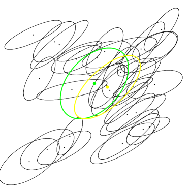
Figure 9: Approximate Fisher centroid of n𝑛n bivariate normals (yellow) vs approximate Hilbert minimax center (green).

Online materials are available at https://franknielsen.github.io/FisherRaoMVN/

References

  • [1] P-A Absil, Robert Mahony, and Rodolphe Sepulchre. Optimization algorithms on matrix manifolds. Princeton University Press, 2008.
  • [2] Layth M Alabdulsada and László Kozma. On non-positive curvature properties of the hilbert metric. The Journal of Geometric Analysis, 29:569–576, 2019.
  • [3] Syed Mumtaz Ali and Samuel D Silvey. A general class of coefficients of divergence of one distribution from another. Journal of the Royal Statistical Society: Series B (Methodological), 28(1):131–142, 1966.
  • [4] Josh Alman and Virginia Vassilevska Williams. A refined laser method and faster matrix multiplication. In Proceedings of the 2021 ACM-SIAM Symposium on Discrete Algorithms (SODA), pages 522–539. SIAM, 2021.
  • [5] Shun-ichi Amari. Information Geometry and Its Applications. Applied Mathematical Sciences. Springer Japan, 2016.
  • [6] Alexandr Andoni. Nearest neighbor search: The old, the new, and the impossible. PhD thesis, Massachusetts Institute of Technology, 2009.
  • [7] Marc Arnaudon and Frank Nielsen. On approximating the Riemannian 111-center. Computational Geometry, 46(1):93–104, 2013.
  • [8] Giacomo Baggio, Augusto Ferrante, and Rodolphe Sepulchre. Conal distances between rational spectral densities. IEEE Transactions on Automatic Control, 64(5):1848–1857, 2018.
  • [9] Grey Ballard, Tamara Kolda, and Todd Plantenga. Efficiently computing tensor eigenvalues on a GPU. In 2011 IEEE International Symposium on Parallel and Distributed Processing Workshops and Phd Forum, pages 1340–1348. IEEE, 2011.
  • [10] Alexandre Barachant, Stéphane Bonnet, Marco Congedo, and Christian Jutten. Multiclass brain–computer interface classification by Riemannian geometry. IEEE Transactions on Biomedical Engineering, 59(4):920–928, 2011.
  • [11] Frédéric Barbaresco. Information geometry of covariance matrix: Cartan-Siegel homogeneous bounded domains, Mostow/Berger fibration and Fréchet median. In Matrix information geometry, pages 199–255. Springer, 2013.
  • [12] Nitin Bhatia et al. Survey of nearest neighbor techniques. arXiv preprint arXiv:1007.0085, 2010.
  • [13] Rajendra Bhatia. Positive definite matrices. In Positive Definite Matrices. Princeton university press, 2009.
  • [14] Rajendra Bhatia and John Holbrook. Noncommutative geometric means. Math. Intelligencer, 28(1):32–39, 2006.
  • [15] Garrett Birkhoff. Extensions of Jentzsch’s theorem. Transactions of the American Mathematical Society, 85(1):219–227, 1957.
  • [16] Martin R Bridson and André Haefliger. Metric spaces of non-positive curvature, volume 319. Springer Science & Business Media, 2013.
  • [17] Jacob Burbea and C Radhakrishna Rao. Entropy differential metric, distance and divergence measures in probability spaces: A unified approach. Journal of Multivariate Analysis, 12(4):575–596, 1982.
  • [18] Yann Cabanes and Frank Nielsen. Classification in the Siegel Space for Vectorial Autoregressive Data. In 5th International Conference on Geometric Science of Information (GSI), pages 693–700. Springer, 2021.
  • [19] Ovidiu Calin and Constantin Udrişte. Geometric modeling in probability and statistics, volume 121. Springer, 2014.
  • [20] Miquel Calvo and Josep M Oller. A distance between multivariate normal distributions based in an embedding into the Siegel group. Journal of multivariate analysis, 35(2):223–242, 1990.
  • [21] Miquel Calvo and Josep Maria Oller. An explicit solution of information geodesic equations for the multivariate normal model. Statistics & Risk Modeling, 9(1-2):119–138, 1991.
  • [22] Chad Carson, Serge Belongie, Hayit Greenspan, and Jitendra Malik. Blobworld: Image segmentation using expectation-maximization and its application to image querying. IEEE Transactions on pattern analysis and machine intelligence, 24(8):1026–1038, 2002.
  • [23] Zeineb Chebbi and Maher Moakher. Means of Hermitian positive-definite matrices based on the log-determinant α𝛼\alpha-divergence function. Linear Algebra and its Applications, 436(7):1872–1889, 2012.
  • [24] Yongxin Chen, Tryphon T Georgiou, and Michele Pavon. Stochastic control liaisons: Richard Sinkhorn meets Gaspard Monge on a Schrodinger bridge. Siam Review, 63(2):249–313, 2021.
  • [25] Guang Cheng, Jeffrey Ho, Hesamoddin Salehian, and Baba C Vemuri. Recursive computation of the Fréchet mean on non-positively curved Riemannian manifolds with applications. Riemannian Computing in Computer Vision, pages 21–43, 2016.
  • [26] Thomas H Cormen, Charles E Leiserson, Ronald L Rivest, and Clifford Stein. Introduction to algorithms. MIT press, 2022.
  • [27] Imre Csiszár. Information-type measures of difference of probability distributions and indirect observation. studia scientiarum Mathematicarum Hungarica, 2:229–318, 1967.
  • [28] Jason Davis and Inderjit Dhillon. Differential entropic clustering of multivariate Gaussians. Advances in Neural Information Processing Systems, 19, 2006.
  • [29] Alberto Dolcetti and Donato Pertici. Elliptic isometries of the manifold of positive definite real matrices with the trace metric. Rendiconti del Circolo Matematico di Palermo Series 2, 70(1):575–592, 2021.
  • [30] Delbert Dueck and Brendan J Frey. Non-metric affinity propagation for unsupervised image categorization. In 2007 IEEE 11th International Conference on Computer Vision, pages 1–8. IEEE, 2007.
  • [31] Poul Svante Eriksen. Geodesics connected with the Fisher metric on the multivariate normal manifold. Technical Report 86-13, Institute of Electronic Systems, Aalborg University Centre, Denmark, 1986.
  • [32] PS Eriksen. Geodesics connected with the Fisher metric on the multivariate normal manifold. In Proceedings of the GST Workshop, Lancaster, UK, pages 28–31, 1987.
  • [33] Shmuel Friedland and Pedro J Freitas. Revisiting the Siegel upper half plane I. Linear algebra and its applications, 376:19–44, 2004.
  • [34] Hitoshi Furuhata, Jun-ichi Inoguchi, and Shimpei Kobayashi. A characterization of the alpha-connections on the statistical manifold of normal distributions. Information Geometry, 4(1):177–188, 2021.
  • [35] Yansong Gao and Pratik Chaudhari. An information-geometric distance on the space of tasks. In International Conference on Machine Learning, pages 3553–3563. PMLR, 2021.
  • [36] Leonor Godinho and José Natário. An introduction to Riemannian geometry. With Applications, 2012.
  • [37] Jacob Goldberger, Hayit K Greenspan, and Jeremie Dreyfuss. Simplifying mixture models using the unscented transform. IEEE Transactions on Pattern Analysis and Machine Intelligence, 30(8):1496–1502, 2008.
  • [38] Teofilo F Gonzalez. Clustering to minimize the maximum intercluster distance. Theoretical computer science, 38:293–306, 1985.
  • [39] Roger B Grosse, Chris J Maddison, and Russ R Salakhutdinov. Annealing between distributions by averaging moments. Advances in Neural Information Processing Systems, 26, 2013.
  • [40] Minyeon Han and Frank C Park. DTI segmentation and fiber tracking using metrics on multivariate normal distributions. Journal of mathematical imaging and vision, 49:317–334, 2014.
  • [41] Alfred O Hero, Bing Ma, Olivier Michel, and John Gorman. Alpha-divergence for classification, indexing and retrieval. Communication and Signal Processing Laboratory, Technical Report CSPL-328, U. Mich, 2001.
  • [42] David Hilbert. Über die Gerade Linie als Kurzeste Verbindung Zweier Punkte. Mathematische Annalen, 46(1):91–96, 1895.
  • [43] Reshad Hosseini and Suvrit Sra. Matrix manifold optimization for Gaussian mixtures. Advances in Neural Information Processing Systems, 28, 2015.
  • [44] Harold Hotelling. Spaces of statistical parameters. Bull. Amer. Math. Soc, 36:191, 1930.
  • [45] Takuro Imai, Akira Takaesu, and Masato Wakayama. Remarks on geodesics for multivariate normal models. Technical report, Faculty of Mathematics, Kyushu University, 2011.
  • [46] A. T. James. The variance information manifold and the functions on it. In Multivariate Analysis–III, pages 157–169. Elsevier, 1973.
  • [47] Anders Karlsson and Guennadi A Noskov. The Hilbert metric and Gromov hyperbolicity. Sonderforschungsbereich 343, 2000.
  • [48] Leonard Kaufman. Partitioning around medoids (program PAM). Finding groups in data, 344:68–125, 1990.
  • [49] Shimpei Kobayashi. Geodesics of multivariate normal distributions and a Toda lattice type Lax pair. arXiv preprint arXiv:2304.12575, 2023.
  • [50] Elon Kohlberg and John W Pratt. The contraction mapping approach to the Perron-Frobenius theory: Why Hilbert’s metric? Mathematics of Operations Research, 7(2):198–210, 1982.
  • [51] Junghyun Kwon, Kyoung Mu Lee, and Frank C Park. Visual tracking via geometric particle filtering on the affine group with optimal importance functions. In 2009 IEEE Conference on Computer Vision and Pattern Recognition, pages 991–998. IEEE, 2009.
  • [52] Serge Lang and Serge Lang. Bruhat-Tits spaces. Math Talks for Undergraduates, pages 79–100, 1999.
  • [53] Stuart Lloyd. Least squares quantization in PCM. IEEE transactions on information theory, 28(2):129–137, 1982.
  • [54] Maher Moakher. A differential geometric approach to the geometric mean of symmetric positive-definite matrices. SIAM journal on matrix analysis and applications, 26(3):735–747, 2005.
  • [55] Yoshimasa Nakamura. Algorithms associated with arithmetic, geometric and harmonic means and integrable systems. Journal of computational and applied mathematics, 131(1-2):161–174, 2001.
  • [56] Frank Nielsen. A Simple Approximation Method for the Fisher–Rao Distance between Multivariate Normal Distributions. Entropy, 25(4):654, 2023.
  • [57] Frank Nielsen and Gaëtan Hadjeres. Monte Carlo information-geometric structures. Geometric Structures of Information, pages 69–103, 2019.
  • [58] Frank Nielsen, Paolo Piro, and Michel Barlaud. Bregman vantage point trees for efficient nearest neighbor queries. In 2009 IEEE International Conference on Multimedia and Expo, pages 878–881. IEEE, 2009.
  • [59] Roger D Nussbaum. Finsler structures for the part metric and Hilbert’s projective metric and applications to ordinary differential equations. Differential and Integral Equations, 7(6):1649–1707, 1994.
  • [60] Atsumi Ohara. Doubly autoparallel structure on positive definite matrices and its applications. In International Conference on Geometric Science of Information, pages 251–260. Springer, 2019.
  • [61] Marion Pilté and Frédéric Barbaresco. Tracking quality monitoring based on information geometry and geodesic shooting. In 2016 17th International Radar Symposium (IRS), pages 1–6. IEEE, 2016.
  • [62] Julianna Pinele, João E Strapasson, and Sueli I R Costa. The Fisher–Rao distance between multivariate normal distributions: Special cases, bounds and applications. Entropy, 22(4):404, 2020.
  • [63] Fatih Porikli, Oncel Tuzel, and Peter Meer. Covariance tracking using model update based on Lie algebra. In 2006 IEEE Computer Society Conference on Computer Vision and Pattern Recognition (CVPR’06), volume 1, pages 728–735. IEEE, 2006.
  • [64] C R Rao. Information and accuracy attainable in the estimation of statistical parameters. Bulletin of the Calcutta Mathematical Society, 37(3):81–91, 1945.
  • [65] Yao Rong, Mengjiao Tang, and Jie Zhou. Intrinsic losses based on information geometry and their applications. Entropy, 19(8):405, 2017.
  • [66] Carl Ludwig Siegel. Symplectic geometry. Academic Press, 1964.
  • [67] Lene Theil Skovgaard. A Riemannian geometry of the multivariate normal model. Scandinavian journal of statistics, pages 211–223, 1984.
  • [68] Suvrit Sra. Positive definite matrices and the S𝑆S-divergence. Proceedings of the American Mathematical Society, 144(7):2787–2797, 2016.
  • [69] João E Strapasson, Julianna Pinele, and Sueli IR Costa. Clustering using the Fisher-Rao distance. In 2016 IEEE Sensor Array and Multichannel Signal Processing Workshop (SAM), pages 1–5. IEEE, 2016.
  • [70] Karl-Theodor Sturm. Probability measures on metric spaces of nonpositive. Heat Kernels and Analysis on Manifolds, Graphs, and Metric Spaces: Lecture Notes from a Quarter Program on Heat Kernels, Random Walks, and Analysis on Manifolds and Graphs: April 16-July 13, 2002, Emile Borel Centre of the Henri Poincaré Institute, Paris, France, 338:357, 2003.
  • [71] Asuka Takatsu. Wasserstein geometry of Gaussian measures. Osaka Journal of Mathematics, 48(4):1005 – 1026, 2011.
  • [72] Luca Trevisan. Lecture notes on graph partitioning, expanders and spectral methods. University of California, Berkeley, 2017.
  • [73] Koji Tsuda, Shotaro Akaho, and Kiyoshi Asai. The em algorithm for kernel matrix completion with auxiliary data. The Journal of Machine Learning Research, 4:67–81, 2003.
  • [74] Oncel Tuzel, Fatih Porikli, and Peter Meer. Pedestrian detection via classification on Riemannian manifolds. IEEE transactions on pattern analysis and machine intelligence, 30(10):1713–1727, 2008.
  • [75] Emo Welzl. Smallest enclosing disks (balls and ellipsoids). In New Results and New Trends in Computer Science, pages 359–370. Springer, 2005.
  • [76] Peter N Yianilos. Data structures and algorithms for nearest neighbor. In Proceedings of the ACM-SIAM Symposium on Discrete algorithms, volume 66, page 311, 1993.
  • [77] Shintaro Yoshizawa and Kunio Tanabe. Dual differential geometry associated with the Kullback-Leibler information on the Gaussian distributions and its 222-parameter deformations. SUT Journal of Mathematics, 35(1):113–137, 1999.
  • [78] Tadashi Yoshizawa. A geometry of parameter space and it’s statistical interpretation. Kokyuroku, pages 103–131, 1972.
  • [79] Kai Zhang and James T Kwok. Simplifying mixture models through function approximation. IEEE Transactions on Neural Networks, 21(4):644–658, 2010.

Appendix A Fisher-Rao geodesics between MVNs with initial value conditions

The Fisher-Rao geodesics γ(t)𝛾𝑡\gamma(t) are smooth curves which are autoparallel with respect to the Levi-Civita connection gsuperscript𝑔\nabla^{g} induced by the metric tensor g𝑔g: γ˙gγ˙=0subscriptsuperscript𝑔˙𝛾˙𝛾0\nabla^{g}_{\dot{\gamma}}\dot{\gamma}=0. On the MVN manifold, the system of Riemannian geodesic equations [67] is

{μ¨Σ˙Σ1μ˙=0,Σ¨+μ˙μ˙Σ˙Σ1Σ˙=0.cases¨𝜇˙ΣsuperscriptΣ1˙𝜇0¨Σ˙𝜇superscript˙𝜇top˙ΣsuperscriptΣ1˙Σ0\left\{\begin{array}[]{lcl}\ddot{\mu}-\dot{\Sigma}\Sigma^{-1}\dot{\mu}&=&0,\\ \ddot{\Sigma}+\dot{\mu}\dot{\mu}^{\top}-\dot{\Sigma}\Sigma^{-1}\dot{\Sigma}&=&0.\end{array}\right.

We may solve the above differential equation system either using initial value conditions (IVPs) by prescribing N0=(μ(0),Σ(0))subscript𝑁0𝜇0Σ0N_{0}=(\mu(0),\Sigma(0)) and a tangent vector N˙(0)=(μ˙(0),Σ˙(0))˙𝑁0˙𝜇0˙Σ0\dot{N}(0)=(\dot{\mu}(0),\dot{\Sigma}(0)), or with boundary value conditions (BVPs) by prescribing N0=(μ(0),Σ(0))subscript𝑁0𝜇0Σ0N_{0}=(\mu(0),\Sigma(0)) and N1=(μ(1),Σ(1))subscript𝑁1𝜇1Σ1N_{1}=(\mu(1),\Sigma(1)). Let γ𝒩Fisher(N0,N˙0;t)superscriptsubscript𝛾𝒩Fishersubscript𝑁0subscript˙𝑁0𝑡\gamma_{\mathcal{N}}^{\mathrm{Fisher}}(N_{0},\dot{N}_{0};t) and γ𝒩Fisher(N0,N01;t)superscriptsubscript𝛾𝒩Fishersubscript𝑁0subscript𝑁01𝑡\gamma_{\mathcal{N}}^{\mathrm{Fisher}}(N_{0},N_{0}1;t) denote these two types of geodesics.

Without loss of generality, let us assume N0=N(0,I)subscript𝑁0𝑁0𝐼N_{0}=N(0,I) (standard normal distribution). The task is to perform geodesic shooting, i.e., calculate N(t)=γ𝒩Fisher(N0,v0;t)𝑁𝑡superscriptsubscript𝛾𝒩Fishersubscript𝑁0subscript𝑣0𝑡N(t)=\gamma_{\mathcal{N}}^{\mathrm{Fisher}}(N_{0},v_{0};t) with some prescribed initial condition (v,S)=γ˙𝒩Fisher(N0,v0;0)TNstd𝑣𝑆superscriptsubscript˙𝛾𝒩Fishersubscript𝑁0subscript𝑣00subscript𝑇𝑁std(v,S)=\dot{\gamma}_{\mathcal{N}}^{\mathrm{Fisher}}(N_{0},v_{0};0)\in T_{N\mathrm{std}}\mathcal{M} and t0𝑡0t\geq 0.

A.1 Eriksen’s homogeneous symmetric space solution

We use the following natural parameterization of the normal distributions:

(ξ=Σ1μ,Ξ=Σ1).formulae-sequence𝜉superscriptΣ1𝜇ΞsuperscriptΣ1\left(\xi=\Sigma^{-1}\mu,\Xi=\Sigma^{-1}\right).

The initial conditions are given by (a=ξ˙(0),B=Ξ˙(0))=γ˙𝒩Fisher(Nstd,v0;0)formulae-sequence𝑎˙𝜉0𝐵˙Ξ0superscriptsubscript˙𝛾𝒩Fishersubscript𝑁stdsubscript𝑣00(a=\dot{\xi}(0),B=\dot{\Xi}(0))=\dot{\gamma}_{\mathcal{N}}^{\mathrm{Fisher}}(N_{\mathrm{std}},v_{0};0) at the standard normal distribution Nstdsubscript𝑁stdN_{\mathrm{std}}. Eriksen’s method proceeds as follows to calculate γ¯FR𝒩(Nstd,v0;t)superscriptsubscript¯𝛾FR𝒩subscript𝑁stdsubscript𝑣0𝑡\underline{\gamma}_{\mathrm{FR}}^{\mathcal{N}}(N_{\mathrm{std}},v_{0};t):

  • Build a (2d+1)×(2d+1)2𝑑12𝑑1(2d+1)\times(2d+1) matrix A𝐴A:

    A=[Ba0a0a0aB].𝐴delimited-[]𝐵𝑎0superscript𝑎top0superscript𝑎top0𝑎𝐵A={\left[\begin{array}[]{lll}-B&a&0\cr a^{\top}&0&-a^{\top}\cr 0&-a&B\end{array}\right]}.
  • Compute matrix M(t)=exp(tA)𝑀𝑡𝑡𝐴M(t)=\exp(tA) for the prescribed value t>0𝑡0t>0. To calculate exp(M)𝑀\exp(M), we first compute the eigen decomposition of AM=Odiag(λ1,,λd)O𝐴𝑀𝑂diagsubscript𝜆1subscript𝜆𝑑superscript𝑂topAM=O\,\mathrm{diag}(\lambda_{1},\ldots,\lambda_{d})\,O^{\top} and then reports Odiag(exp(λ1),,exp(λd))O𝑂diagsubscript𝜆1subscript𝜆𝑑superscript𝑂topO\,\mathrm{diag}(\exp(\lambda_{1}),\ldots,\exp(\lambda_{d}))\,O^{\top}.

  • Extract (ξ(t),Ξ(t))𝜉𝑡Ξ𝑡(\xi(t),\Xi(t)) from M(t)𝑀𝑡M(t) and convert to (μ(t),Σ(t))𝜇𝑡Σ𝑡(\mu(t),\Sigma(t)):

    Σ(t)Σ𝑡\displaystyle\Sigma(t) =\displaystyle= [M(t)]1:d,1:d1,subscriptsuperscriptdelimited-[]𝑀𝑡1:1𝑑1:𝑑\displaystyle[M(t)]^{-1}_{1:d,1:d},
    μ(t)𝜇𝑡\displaystyle\mu(t) =\displaystyle= Σ(t)[M(t)]1:d,d+1.Σ𝑡subscriptdelimited-[]𝑀𝑡:1𝑑𝑑1\displaystyle\Sigma(t)[M(t)]_{1:d,d+1}.
  • Report γ¯FR𝒩(Nstd,v0;t)=(μ(t),Σ(t))superscriptsubscript¯𝛾FR𝒩subscript𝑁stdsubscript𝑣0𝑡𝜇𝑡Σ𝑡\underline{\gamma}_{\mathrm{FR}}^{\mathcal{N}}(N_{\mathrm{std}},v_{0};t)=(\mu(t),\Sigma(t)).

Eriksen’s method yields a pregeodesic and not a geodesic. For geodesics, we have the following Fisher-Rao distance property ρ𝒩(γFR𝒩(Nstd,v0;s),γFR𝒩(Nstd,v0;t))=|st|ρ𝒩(γFR𝒩(N0,N1)\rho_{\mathcal{N}}({\gamma}_{\mathrm{FR}}^{\mathcal{N}}(N_{\mathrm{std}},v_{0};s),{\gamma}_{\mathrm{FR}}^{\mathcal{N}}(N_{\mathrm{std}},v_{0};t))=|s-t|\,\rho_{\mathcal{N}}({\gamma}_{\mathrm{FR}}^{\mathcal{N}}(N_{0},N_{1}) where N0=Nstdsubscript𝑁0subscript𝑁stdN_{0}=N_{\mathrm{std}} and N1=γFR𝒩(Nstd,v0;1)subscript𝑁1superscriptsubscript𝛾FR𝒩subscript𝑁stdsubscript𝑣01N_{1}={\gamma}_{\mathrm{FR}}^{\mathcal{N}}(N_{\mathrm{std}},v_{0};1).

A.2 Calvo and Oller’s direction solution

We report the solution given in [21] which relies on the following natural parameterization of the normal distributions

(ξ=Σ1μ,Ξ=Σ1).formulae-sequence𝜉superscriptΣ1𝜇ΞsuperscriptΣ1\left(\xi=\Sigma^{-1}\mu,\Xi=\Sigma^{-1}\right).

The initial conditions are given by (a=ξ˙(0),B=Ξ˙(0))=γ˙𝒩Fisher(N0,v0;0)formulae-sequence𝑎˙𝜉0𝐵˙Ξ0superscriptsubscript˙𝛾𝒩Fishersubscript𝑁0subscript𝑣00(a=\dot{\xi}(0),B=\dot{\Xi}(0))=\dot{\gamma}_{\mathcal{N}}^{\mathrm{Fisher}}(N_{0},v_{0};0).

The method of [21] first calculate those quantities:

B𝐵\displaystyle B =\displaystyle= Ξ(0)12Ξ˙(0)Ξ(0)12,Ξsuperscript012˙Ξ0Ξsuperscript012\displaystyle-\Xi(0)^{-\frac{1}{2}}\,\dot{\Xi}(0)\,\Xi(0)^{-\frac{1}{2}},
a𝑎\displaystyle a =\displaystyle= Ξ(0)12ξ˙(0)+BΞ012ξ(0),Ξsuperscript012˙𝜉0𝐵superscriptsubscriptΞ012𝜉0\displaystyle\Xi(0)^{-\frac{1}{2}}\dot{\xi}(0)+B\Xi_{0}^{-\frac{1}{2}}\xi(0),
G𝐺\displaystyle G =\displaystyle= (B2+2aa)12.superscriptsuperscript𝐵22𝑎superscript𝑎top12\displaystyle(B^{2}+2aa^{\top})^{\frac{1}{2}}.

Furthermore, let G=G1superscript𝐺superscript𝐺1G^{\dagger}=G^{-1} when G𝐺G is invertible or G=(GG)1Gsuperscript𝐺superscriptsuperscript𝐺top𝐺1superscript𝐺topG^{\dagger}=(G^{\top}G)^{-1}G^{\top} the Moore-Penrose generalized pseudo-inverse matrix of G𝐺G otherwise (or any kind of generalized matrix inverse Gsuperscript𝐺G^{-} [21], see).

Then we have (ξ(t),Ξ(t))=γ𝒩Fisher(N0,v0;t)𝜉𝑡Ξ𝑡superscriptsubscript𝛾𝒩Fishersubscript𝑁0subscript𝑣0𝑡(\xi(t),\Xi(t))=\gamma_{\mathcal{N}}^{\mathrm{Fisher}}(N_{0},v_{0};t) with

Ξ(t)Ξ𝑡\displaystyle\Xi(t) =\displaystyle= Ξ(0)12R(t)R(t)Ξ(0)12,Ξsuperscript012𝑅𝑡𝑅superscript𝑡topΞsuperscript012\displaystyle\Xi(0)^{\frac{1}{2}}\,R(t)R(t)^{\top}\,\Xi(0)^{\frac{1}{2}},
ξ(t)𝜉𝑡\displaystyle\xi(t) =\displaystyle= 2Ξ(0)12R(t)Sinh(12Gt)Ga+Ξ(t)Ξ1(0)ξ(0),2Ξsuperscript012𝑅𝑡Sinh12𝐺𝑡superscript𝐺𝑎Ξ𝑡superscriptΞ10𝜉0\displaystyle 2\Xi(0)^{\frac{1}{2}}\,R(t)\mathrm{Sinh}\left(\frac{1}{2}Gt\right)G^{\dagger}a+\Xi(t)\Xi^{-1}(0)\xi(0),

and

R(t)=Cosh(12Gt)BGSinh(12Gt).𝑅𝑡Cosh12𝐺𝑡𝐵superscript𝐺Sinh12𝐺𝑡R(t)=\mathrm{Cosh}\left(\frac{1}{2}Gt\right)-BG^{\dagger}\mathrm{Sinh}\left(\frac{1}{2}Gt\right).

The matrix hyperbolic cosine and sinus functions of M𝑀M are calculated from the eigen decomposition of M=Odiag(λ1,,λd)O𝑀𝑂diagsubscript𝜆1subscript𝜆𝑑superscript𝑂topM=O\,\mathrm{diag}(\lambda_{1},\ldots,\lambda_{d})\,O^{\top} as follows:

Sinh(M)Sinh𝑀\displaystyle\mathrm{Sinh}(M) =\displaystyle= Odiag(sinh(λ1),,sinh(λd))O,sinh(u)=eueu2=i=0u2i+1(2i+1)!,𝑂diagsinhsubscript𝜆1sinhsubscript𝜆𝑑superscript𝑂topsinh𝑢superscript𝑒𝑢superscript𝑒𝑢2superscriptsubscript𝑖0superscript𝑢2𝑖12𝑖1\displaystyle O\,\mathrm{diag}(\mathrm{sinh}(\lambda_{1}),\ldots,\mathrm{sinh}(\lambda_{d}))\,O^{\top},\quad\mathrm{sinh}(u)=\frac{e^{u}-e^{-u}}{2}=\sum_{i=0}^{\infty}\frac{u^{2i+1}}{(2i+1)!},
Cosh(M)Cosh𝑀\displaystyle\mathrm{Cosh}(M) =\displaystyle= Odiag(cosh(λ1),,cosh(λd))O,cosh(u)=eu+eu2=i=0u2i(2i)!.𝑂diagcoshsubscript𝜆1coshsubscript𝜆𝑑superscript𝑂topcosh𝑢superscript𝑒𝑢superscript𝑒𝑢2superscriptsubscript𝑖0superscript𝑢2𝑖2𝑖\displaystyle O\,\mathrm{diag}(\mathrm{cosh}(\lambda_{1}),\ldots,\mathrm{cosh}(\lambda_{d}))\,O^{\top},\quad\mathrm{cosh}(u)=\frac{e^{u}+e^{-u}}{2}=\sum_{i=0}^{\infty}\frac{u^{2i}}{(2i)!}.

For the general case γ𝒩Fisher(N,v0;t)superscriptsubscript𝛾𝒩Fisher𝑁subscript𝑣0𝑡\gamma_{\mathcal{N}}^{\mathrm{Fisher}}(N,v_{0};t) with arbitrary N=(Σ,μ)𝑁Σ𝜇N=(\Sigma,\mu), we use the affine equivariance property of the Fisher-Rao geodesics with P=Σ12𝑃superscriptΣ12P=\Sigma^{-\frac{1}{2}}:

γ𝒩Fisher(N,v0;t)=(Pμ,P1).γ𝒩Fisher(Nstd,(Pa,PBP);t).formulae-sequencesuperscriptsubscript𝛾𝒩Fisher𝑁subscript𝑣0𝑡𝑃𝜇superscript𝑃1superscriptsubscript𝛾𝒩Fishersubscript𝑁std𝑃𝑎𝑃𝐵superscript𝑃top𝑡\gamma_{\mathcal{N}}^{\mathrm{Fisher}}(N,v_{0};t)=(-P\mu,P^{-1}).\gamma_{\mathcal{N}}^{\mathrm{Fisher}}(N_{\mathrm{std}},(Pa,-PBP^{\top});t). (25)

Figure 10 displays several examples of geodesics from the standard normal distribution with various initial value conditions.
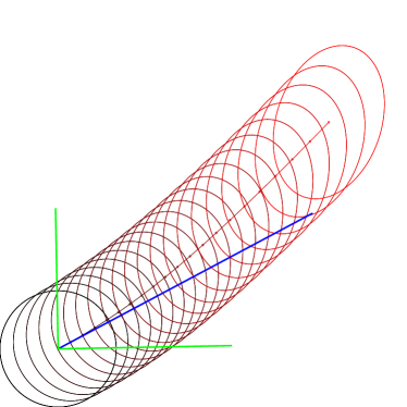
Refer to caption Refer to caption
Figure 10: Examples of Fisher-Rao geodesics (μ(t),Σ(t))𝜇𝑡Σ𝑡(\mu(t),\Sigma(t)) emanating from the standard bivariate normal distribution (μ(0),Σ(0))=N(0,I)𝜇0Σ0𝑁0𝐼(\mu(0),\Sigma(0))=N(0,I) with initial value conditions (μ˙(0),Σ˙(0))˙𝜇0˙Σ0(\dot{\mu}(0),\dot{\Sigma}(0)). Vectors μ˙(0)˙𝜇0\dot{\mu}(0) are shown in blue and symmetric matrices Σ˙(0)=λ1v1v1+λ2v2v2˙Σ0subscript𝜆1subscript𝑣1superscriptsubscript𝑣1topsubscript𝜆2subscript𝑣2superscriptsubscript𝑣2top\dot{\Sigma}(0)=\lambda_{1}v_{1}v_{1}^{\top}+\lambda_{2}v_{2}v_{2}^{\top} are visualized by their two scaled eigenvectors λ1v1subscript𝜆1subscript𝑣1\lambda_{1}v_{1} and λ2v2subscript𝜆2subscript𝑣2\lambda_{2}v_{2} shown in green.

The geodesics with initial values let us define the Riemannian exponential map exp:TN:subscript𝑇𝑁\exp:T_{N}\mathcal{M}\rightarrow\mathcal{M}:

expN(v)=γ𝒩Fisher(N,v;1).subscript𝑁𝑣superscriptsubscript𝛾𝒩Fisher𝑁𝑣1\exp_{N}(v)=\gamma_{\mathcal{N}}^{\mathrm{Fisher}}(N,v;1).

The inverse map is the Riemannian logarithm map. In a geodesically complete manifold (e.g., 𝒩μsubscript𝒩𝜇\mathcal{N}_{\mu}), we can express the Fisher-Rao distance as:

ρ𝒩(N1,N2)=LogN1(N2)N1.subscript𝜌𝒩subscript𝑁1subscript𝑁2subscriptnormsubscriptLogsubscript𝑁1subscript𝑁2subscript𝑁1\rho_{\mathcal{N}}(N_{1},N_{2})=\|{\mathrm{Log}}_{N_{1}}(N_{2})\|_{N_{1}}.

Thus computing the Fisher-Rao distance can be done by computing the Riemannian MVN logarithm.

Appendix B Proof of square root of Jeffreys upper bound

Let us prove that the Fisher-Rao distance between normal distributions is upper bounded by the square root of the Jeffreys divergence:

ρ𝒩(N1,N2)DJ(N1,N2).subscript𝜌𝒩subscript𝑁1subscript𝑁2subscript𝐷𝐽subscript𝑁1subscript𝑁2\rho_{\mathcal{N}}(N_{1},N_{2})\leq\sqrt{D_{J}(N_{1},N_{2})}.
Property 2.

We have

DJ[pλ1,pλ2]=01ds𝒩2(γ𝒩m(pλ1,pλ2;t))dt=01ds𝒩2(γ𝒩e(pλ1,pλ2;t))dt.subscript𝐷𝐽subscript𝑝subscript𝜆1subscript𝑝subscript𝜆2superscriptsubscript01differential-dsuperscriptsubscript𝑠𝒩2subscriptsuperscript𝛾𝑚𝒩subscript𝑝subscript𝜆1subscript𝑝subscript𝜆2𝑡differential-d𝑡superscriptsubscript01differential-dsuperscriptsubscript𝑠𝒩2subscriptsuperscript𝛾𝑒𝒩subscript𝑝subscript𝜆1subscript𝑝subscript𝜆2𝑡differential-d𝑡D_{J}[p_{\lambda_{1}},p_{\lambda_{2}}]=\int_{0}^{1}\mathrm{d}s_{\mathcal{N}}^{2}(\gamma^{m}_{\mathcal{N}}(p_{\lambda_{1}},p_{\lambda_{2}};t))\mathrm{d}t=\int_{0}^{1}\mathrm{d}s_{\mathcal{N}}^{2}(\gamma^{e}_{\mathcal{N}}(p_{\lambda_{1}},p_{\lambda_{2}};t))\mathrm{d}t.

Let SF(θ1;θ2)=BF(θ1:θ2)+BF(θ2:θ1)S_{F}(\theta_{1};\theta_{2})=B_{F}(\theta_{1}:\theta_{2})+B_{F}(\theta_{2}:\theta_{1}) be a symmetrized Bregman divergence. Let ds2=dθ2F(θ)dθdsuperscript𝑠2dsuperscript𝜃topsuperscript2𝐹𝜃d𝜃\mathrm{d}s^{2}=\mathrm{d}\theta^{\top}\nabla^{2}F(\theta)\mathrm{d}\theta denote the squared length element on the Bregman manifold and denote by γ(t)𝛾𝑡\gamma(t) and γ(t)superscript𝛾𝑡\gamma^{*}(t) the dual geodesics connecting θ1subscript𝜃1\theta_{1} to θ2subscript𝜃2\theta_{2}. We can express SF(θ1;θ2)subscript𝑆𝐹subscript𝜃1subscript𝜃2S_{F}(\theta_{1};\theta_{2}) as integral energies on dual geodesics:

Property 3.

We have SF(θ1;θ2)=01ds2(γ(t))dt=01ds2(γ(t))dtsubscript𝑆𝐹subscript𝜃1subscript𝜃2superscriptsubscript01differential-dsuperscript𝑠2𝛾𝑡differential-d𝑡superscriptsubscript01differential-dsuperscript𝑠2superscript𝛾𝑡differential-d𝑡S_{F}(\theta_{1};\theta_{2})=\int_{0}^{1}\mathrm{d}s^{2}(\gamma(t))\mathrm{d}t=\int_{0}^{1}\mathrm{d}s^{2}(\gamma^{*}(t))\mathrm{d}t.

Proof.

The proof that the symmetrized Bregman divergence amount to these energy integrals is based on the first-order and second-order directional derivatives. The first-order directional derivative uF(θ)subscript𝑢𝐹𝜃\nabla_{u}F(\theta) with respect to vector u𝑢u is defined by

uF(θ)=limt0F(θ+tv)F(θ)t=vF(θ).subscript𝑢𝐹𝜃subscript𝑡0𝐹𝜃𝑡𝑣𝐹𝜃𝑡superscript𝑣top𝐹𝜃\nabla_{u}F(\theta)=\lim_{t\rightarrow 0}\frac{F(\theta+tv)-F(\theta)}{t}=v^{\top}\nabla F(\theta).

The second-order directional derivatives u,v2F(θ)superscriptsubscript𝑢𝑣2𝐹𝜃\nabla_{u,v}^{2}F(\theta) is

u,v2F(θ)superscriptsubscript𝑢𝑣2𝐹𝜃\displaystyle\nabla_{u,v}^{2}F(\theta) =\displaystyle= uvF(θ),subscript𝑢subscript𝑣𝐹𝜃\displaystyle\nabla_{u}\nabla_{v}F(\theta),
=\displaystyle= limt0vF(θ+tu)vF(θ)t,subscript𝑡0superscript𝑣top𝐹𝜃𝑡𝑢superscript𝑣top𝐹𝜃𝑡\displaystyle\lim_{t\rightarrow 0}\frac{v^{\top}\nabla F(\theta+tu)-v^{\top}\nabla F(\theta)}{t},
=\displaystyle= u2F(θ)v.superscript𝑢topsuperscript2𝐹𝜃𝑣\displaystyle u^{\top}\nabla^{2}F(\theta)v.

Now consider the squared length element ds2(γ(t))dsuperscript𝑠2𝛾𝑡\mathrm{d}s^{2}(\gamma(t)) on the primal geodesic γ(t)𝛾𝑡\gamma(t) expressed using the primal coordinate system θ𝜃\theta: ds2(γ(t))=dθ(t)2F(θ(t))dθ(t)dsuperscript𝑠2𝛾𝑡d𝜃superscript𝑡topsuperscript2𝐹𝜃𝑡d𝜃𝑡\mathrm{d}s^{2}(\gamma(t))=\mathrm{d}\theta(t)^{\top}\nabla^{2}F(\theta(t))\mathrm{d}\theta(t) with θ(γ(t))=θ1+t(θ2θ1)𝜃𝛾𝑡subscript𝜃1𝑡subscript𝜃2subscript𝜃1\theta(\gamma(t))=\theta_{1}+t(\theta_{2}-\theta_{1}) and dθ(t)=θ2θ1d𝜃𝑡subscript𝜃2subscript𝜃1\mathrm{d}\theta(t)=\theta_{2}-\theta_{1}. Let us express the ds2(γ(t))dsuperscript𝑠2𝛾𝑡\mathrm{d}s^{2}(\gamma(t)) using the second-order directional derivative:

ds2(γ(t))=θ2θ12F(θ(t)).dsuperscript𝑠2𝛾𝑡subscriptsuperscript2subscript𝜃2subscript𝜃1𝐹𝜃𝑡\mathrm{d}s^{2}(\gamma(t))=\nabla^{2}_{\theta_{2}-\theta_{1}}F(\theta(t)).

Thus we have 01ds2(γ(t))dt=[θ2θ1F(θ(t))]01superscriptsubscript01differential-dsuperscript𝑠2𝛾𝑡differential-d𝑡superscriptsubscriptdelimited-[]subscriptsubscript𝜃2subscript𝜃1𝐹𝜃𝑡01\int_{0}^{1}\mathrm{d}s^{2}(\gamma(t))\mathrm{d}t=[\nabla_{\theta_{2}-\theta_{1}}F(\theta(t))]_{0}^{1}, where the first-order directional derivative is θ2θ1F(θ(t))=(θ2θ1)F(θ(t))subscriptsubscript𝜃2subscript𝜃1𝐹𝜃𝑡superscriptsubscript𝜃2subscript𝜃1top𝐹𝜃𝑡\nabla_{\theta_{2}-\theta_{1}}F(\theta(t))=(\theta_{2}-\theta_{1})^{\top}\nabla F(\theta(t)). Therefore we get 01ds2(γ(t))dt=(θ2θ1)(F(θ2)F(θ1))=SF(θ1;θ2)superscriptsubscript01differential-dsuperscript𝑠2𝛾𝑡differential-d𝑡superscriptsubscript𝜃2subscript𝜃1top𝐹subscript𝜃2𝐹subscript𝜃1subscript𝑆𝐹subscript𝜃1subscript𝜃2\int_{0}^{1}\mathrm{d}s^{2}(\gamma(t))\mathrm{d}t=(\theta_{2}-\theta_{1})^{\top}(\nabla F(\theta_{2})-\nabla F(\theta_{1}))=S_{F}(\theta_{1};\theta_{2}).

Similarly, we express the squared length element ds2(γ(t))dsuperscript𝑠2superscript𝛾𝑡\mathrm{d}s^{2}(\gamma^{*}(t)) using the dual coordinate system η𝜂\eta as the second-order directional derivative of F(η(t))superscript𝐹𝜂𝑡F^{*}(\eta(t)) with η(γ(t))=η1+t(η2η1)𝜂superscript𝛾𝑡subscript𝜂1𝑡subscript𝜂2subscript𝜂1\eta(\gamma^{*}(t))=\eta_{1}+t(\eta_{2}-\eta_{1}):

ds2(γ(t))=η2η12F(η(t)).dsuperscript𝑠2superscript𝛾𝑡subscriptsuperscript2subscript𝜂2subscript𝜂1superscript𝐹𝜂𝑡\mathrm{d}s^{2}(\gamma^{*}(t))=\nabla^{2}_{\eta_{2}-\eta_{1}}F^{*}(\eta(t)).

Therefore, we have 01ds2(γ(t))dt=[η2η1F(η(t))]01=SF(η1;η2)superscriptsubscript01differential-dsuperscript𝑠2superscript𝛾𝑡differential-d𝑡superscriptsubscriptdelimited-[]subscriptsubscript𝜂2subscript𝜂1superscript𝐹𝜂𝑡01subscript𝑆superscript𝐹subscript𝜂1𝜂2\int_{0}^{1}\mathrm{d}s^{2}(\gamma^{*}(t))\mathrm{d}t=[\nabla_{\eta_{2}-\eta_{1}}F^{*}(\eta(t))]_{0}^{1}=S_{F^{*}}(\eta_{1};\eta 2). Since SF(η1;η2)=SF(θ1;θ2)subscript𝑆superscript𝐹subscript𝜂1subscript𝜂2subscript𝑆𝐹subscript𝜃1subscript𝜃2S_{F^{*}}(\eta_{1};\eta_{2})=S_{F}(\theta_{1};\theta_{2}), we conclude that

SF(θ1;θ2)=01ds2(γ(t))dt=01ds2(γ(t))dtsubscript𝑆𝐹subscript𝜃1subscript𝜃2superscriptsubscript01differential-dsuperscript𝑠2𝛾𝑡differential-d𝑡superscriptsubscript01differential-dsuperscript𝑠2superscript𝛾𝑡differential-d𝑡S_{F}(\theta_{1};\theta_{2})=\int_{0}^{1}\mathrm{d}s^{2}(\gamma(t))\mathrm{d}t=\int_{0}^{1}\mathrm{d}s^{2}(\gamma^{*}(t))\mathrm{d}t

Note that in 1D, both pregeodesics γ(t)𝛾𝑡\gamma(t) and γ(t)superscript𝛾𝑡\gamma^{*}(t) coincide. We have ds2(t)=(θ2θ1)2f′′(θ(t))=(η2η1)f′′(η(t))dsuperscript𝑠2𝑡superscriptsubscript𝜃2subscript𝜃12superscript𝑓′′𝜃𝑡subscript𝜂2subscript𝜂1superscriptsuperscript𝑓′′𝜂𝑡\mathrm{d}s^{2}(t)=(\theta_{2}-\theta_{1})^{2}f^{\prime\prime}(\theta(t))=(\eta_{2}-\eta_{1}){f^{*}}^{\prime\prime}(\eta(t)) so that we check that SF(θ1;θ2)=01ds2(γ(t))dt=(θ2θ1)[f(θ(t))]01=(η2η1)[f(η(t))]01=(η2η1)(θ2θ2)subscript𝑆𝐹subscript𝜃1subscript𝜃2superscriptsubscript01differential-dsuperscript𝑠2𝛾𝑡differential-d𝑡subscript𝜃2subscript𝜃1superscriptsubscriptdelimited-[]superscript𝑓𝜃𝑡01subscript𝜂2subscript𝜂1superscriptsubscriptdelimited-[]superscriptsuperscript𝑓𝜂𝑡01subscript𝜂2subscript𝜂1subscript𝜃2subscript𝜃2S_{F}(\theta_{1};\theta_{2})=\int_{0}^{1}\mathrm{d}s^{2}(\gamma(t))\mathrm{d}t=(\theta_{2}-\theta_{1})[f^{\prime}(\theta(t))]_{0}^{1}=(\eta_{2}-\eta_{1})[{f^{*}}^{\prime}(\eta(t))]_{0}^{1}=(\eta_{2}-\eta_{1})(\theta_{2}-\theta_{2}). ∎

Property 4 ([5]).

We have

DJ[pλ1,pλ2]=01ds𝒩2(γ𝒩m(pλ1,pλ2;t))dt=01ds𝒩2(γ𝒩e(pλ1,pλ2;t))dt.subscript𝐷𝐽subscript𝑝subscript𝜆1subscript𝑝subscript𝜆2superscriptsubscript01differential-dsuperscriptsubscript𝑠𝒩2subscriptsuperscript𝛾𝑚𝒩subscript𝑝subscript𝜆1subscript𝑝subscript𝜆2𝑡differential-d𝑡superscriptsubscript01differential-dsuperscriptsubscript𝑠𝒩2subscriptsuperscript𝛾𝑒𝒩subscript𝑝subscript𝜆1subscript𝑝subscript𝜆2𝑡differential-d𝑡D_{J}[p_{\lambda_{1}},p_{\lambda_{2}}]=\int_{0}^{1}\mathrm{d}s_{\mathcal{N}}^{2}(\gamma^{m}_{\mathcal{N}}(p_{\lambda_{1}},p_{\lambda_{2}};t))\mathrm{d}t=\int_{0}^{1}\mathrm{d}s_{\mathcal{N}}^{2}(\gamma^{e}_{\mathcal{N}}(p_{\lambda_{1}},p_{\lambda_{2}};t))\mathrm{d}t.
Proof.

Let us report a proof of this remarkable fact in the general setting of Bregman manifolds. Indeed, since

DJ[pλ1,pλ2]=DKL[pλ1:pλ2]+DKL[pλ2:pλ1],D_{J}[p_{\lambda_{1}},p_{\lambda_{2}}]=D_{\mathrm{KL}}[p_{\lambda_{1}}:p_{\lambda_{2}}]+D_{\mathrm{KL}}[p_{\lambda_{2}}:p_{\lambda_{1}}],

and DKL[pλ1:pλ2]=BF(θ(λ2):θ(λ1))D_{\mathrm{KL}}[p_{\lambda_{1}}:p_{\lambda_{2}}]=B_{F}(\theta(\lambda_{2}):\theta(\lambda_{1})), where BFsubscript𝐵𝐹B_{F} denotes the Bregman divergence induced by the cumulant function of the multivariate normals and θ(λ)𝜃𝜆\theta(\lambda) is the natural parameter corresponding to λ𝜆\lambda, we have

DJ[pλ1,pλ2]subscript𝐷𝐽subscript𝑝subscript𝜆1subscript𝑝subscript𝜆2\displaystyle D_{J}[p_{\lambda_{1}},p_{\lambda_{2}}] =\displaystyle= BF(θ1:θ2)+BF(θ2:θ1),\displaystyle B_{F}(\theta_{1}:\theta_{2})+B_{F}(\theta_{2}:\theta_{1}),
=\displaystyle= SF(θ1;θ2)=(θ2θ1)(η2η1)=SF(η1;η2),subscript𝑆𝐹subscript𝜃1subscript𝜃2superscriptsubscript𝜃2subscript𝜃1topsubscript𝜂2subscript𝜂1subscript𝑆superscript𝐹subscript𝜂1subscript𝜂2\displaystyle S_{F}(\theta_{1};\theta_{2})=(\theta_{2}-\theta_{1})^{\top}(\eta_{2}-\eta_{1})=S_{F^{*}}(\eta_{1};\eta_{2}),

where η=F(θ)𝜂𝐹𝜃\eta=\nabla F(\theta) and θ=F(η)𝜃superscript𝐹𝜂\theta=\nabla F^{*}(\eta) denote the dual parameterizations obtained by the Legendre-Fenchel convex conjugate F(η)superscript𝐹𝜂F^{*}(\eta) of F(θ)𝐹𝜃F(\theta). Moreover, we have F(η)=h(pμ,Σ)superscript𝐹𝜂subscript𝑝𝜇ΣF^{*}(\eta)=-h(p_{\mu,\Sigma}) [5], i.e., the convex conjugate function is Shannon negentropy.

Then we conclude by using the fact that SF(θ1;θ2)=01ds2(γ(t))dt=01ds2(γ(t))dtsubscript𝑆𝐹subscript𝜃1subscript𝜃2superscriptsubscript01differential-dsuperscript𝑠2𝛾𝑡differential-d𝑡superscriptsubscript01differential-dsuperscript𝑠2superscript𝛾𝑡differential-d𝑡S_{F}(\theta_{1};\theta_{2})=\int_{0}^{1}\mathrm{d}s^{2}(\gamma(t))\mathrm{d}t=\int_{0}^{1}\mathrm{d}s^{2}(\gamma^{*}(t))\mathrm{d}t, i.e., the symmetrized Bregman divergence amounts to integral energies on dual geodesics on a Bregman manifold. The proof of this general property is reported in Appendix B. ∎

Property 5 (Fisher–Rao upper bound).

The Fisher-Rao distance between normal distributions is upper bounded by the square root of the Jeffreys divergence: ρ𝒩(N1,N2)DJ(N1,N2)subscript𝜌𝒩subscript𝑁1subscript𝑁2subscript𝐷𝐽subscript𝑁1subscript𝑁2\rho_{\mathcal{N}}(N_{1},N_{2})\leq\sqrt{D_{J}(N_{1},N_{2})}.

Proof.

Consider the Cauchy-Schwarz inequality for positive functions f(t)𝑓𝑡f(t) and g(t)𝑔𝑡g(t):

01f(t)g(t)dt(01f(t)2dt)(01g(t)2dt),superscriptsubscript01𝑓𝑡𝑔𝑡differential-d𝑡superscriptsubscript01𝑓superscript𝑡2differential-d𝑡superscriptsubscript01𝑔superscript𝑡2differential-d𝑡\int_{0}^{1}f(t)\,g(t)\mathrm{d}t\leq\sqrt{(\int_{0}^{1}f(t)^{2}\mathrm{d}t)\,(\int_{0}^{1}g(t)^{2}\mathrm{d}t)},

and let f(t)=ds𝒩(γ𝒩c(pλ1,pλ2;t)f(t)=\mathrm{d}s_{\mathcal{N}}(\gamma^{c}_{\mathcal{N}}(p_{\lambda_{1}},p_{\lambda_{2}};t) and g(t)=1𝑔𝑡1g(t)=1. Then we get:

(01ds𝒩(γ𝒩c(pλ1,pλ2;t)dt)2(01ds𝒩2(γ𝒩c(pλ1,pλ2;t)dt)(0112dt=1).\left(\int_{0}^{1}\mathrm{d}s_{\mathcal{N}}(\gamma^{c}_{\mathcal{N}}(p_{\lambda_{1}},p_{\lambda_{2}};t)\mathrm{d}t\right)^{2}\leq\left(\int_{0}^{1}\mathrm{d}s_{\mathcal{N}}^{2}(\gamma^{c}_{\mathcal{N}}(p_{\lambda_{1}},p_{\lambda_{2}};t)\mathrm{d}t\right)\left(\underbrace{\int_{0}^{1}1^{2}\mathrm{d}t}_{=1}\right).

Furthermore since by definition of γ𝒩FRsuperscriptsubscript𝛾𝒩FR\gamma_{\mathcal{N}}^{\mathrm{FR}}, we have

01ds𝒩(γ𝒩c(pλ1,pλ2;t)dt01ds𝒩(γ𝒩FR(pλ1,pλ2;t)dt=:ρ𝒩(N1,N2).\int_{0}^{1}\mathrm{d}s_{\mathcal{N}}(\gamma^{c}_{\mathcal{N}}(p_{\lambda_{1}},p_{\lambda_{2}};t)\mathrm{d}t\geq\int_{0}^{1}\mathrm{d}s_{\mathcal{N}}(\gamma^{\mathrm{FR}}_{\mathcal{N}}(p_{\lambda_{1}},p_{\lambda_{2}};t)\mathrm{d}t=:\rho_{\mathcal{N}}(N_{1},N_{2}).

It follows for c=γ𝒩e𝑐subscriptsuperscript𝛾𝑒𝒩c=\gamma^{e}_{\mathcal{N}} (i.e., e𝑒e-geodesic) using Property 4 that we have:

ρ𝒩(N1,N2)201ds𝒩2(γ𝒩e(pλ1,pλ2;t)dt=DJ(N1,N2).\rho_{\mathcal{N}}(N_{1},N_{2})^{2}\leq\int_{0}^{1}\mathrm{d}s_{\mathcal{N}}^{2}(\gamma^{e}_{\mathcal{N}}(p_{\lambda_{1}},p_{\lambda_{2}};t)\mathrm{d}t=D_{J}(N_{1},N_{2}).

Thus we conclude that ρ𝒩(N1,N2)DJ(N1,N2)subscript𝜌𝒩subscript𝑁1subscript𝑁2subscript𝐷𝐽subscript𝑁1subscript𝑁2\rho_{\mathcal{N}}(N_{1},N_{2})\leq\sqrt{D_{J}(N_{1},N_{2})}.

Note that in Riemannian geometry, a curve γ𝛾\gamma minimizes the energy E(γ)=01γ˙(t)2dt𝐸𝛾superscriptsubscript01superscriptnorm˙𝛾𝑡2differential-d𝑡E(\gamma)=\int_{0}^{1}\|\dot{\gamma}(t)\|^{2}\mathrm{d}t if it minimizes the length Len(γ)=01γ˙(t)dtLen𝛾superscriptsubscript01norm˙𝛾𝑡differential-d𝑡\mathrm{Len}(\gamma)=\int_{0}^{1}\|\dot{\gamma}(t)\|\mathrm{d}t and γ˙(t)norm˙𝛾𝑡\|\dot{\gamma}(t)\| is constant. Using Cauchy-Schwartz inequality, we can show that Len(γ)E(γ)Len𝛾𝐸𝛾\mathrm{Len}(\gamma)\leq E(\gamma). ∎

Appendix C Riemannian SPD geodesic and the arithmetic-harmonic inductive mean

The Riemannian SPD geodesic γ(X,Y;t)𝛾𝑋𝑌𝑡\gamma(X,Y;t) joining two SPD matrices X𝑋X and Y𝑌Y with respect to the trace metric can be expressed using the weighted matrix geometric mean:

γ(X,Y;t)=X#tY=X12(X12YX12)tX12.𝛾𝑋𝑌𝑡𝑋subscript#𝑡𝑌superscript𝑋12superscriptsuperscript𝑋12𝑌superscript𝑋12𝑡superscript𝑋12\gamma(X,Y;t)=X\#_{t}Y=X^{\frac{1}{2}}\,\left(X^{-\frac{1}{2}}\,Y\,X^{-\frac{1}{2}}\right)^{t}\,X^{\frac{1}{2}}. (26)

We denote by X#Y=X#12Y=𝑋#𝑌𝑋subscript#12𝑌absentX\#Y=X\#_{\frac{1}{2}}Y=. For t(0,1)𝑡01t\in(0,1), X#tY𝑋subscript#𝑡𝑌X\#_{t}Y defines a matrix mean [14] of X𝑋X and Y𝑌Y which is asymmetric when t12𝑡12t\not=\frac{1}{2}.

The matrix geometric mean can be computed inductively using the following arithmetic-harmonic sequence:

At+1subscript𝐴𝑡1\displaystyle A_{t+1} =\displaystyle= A(At,Ht),𝐴subscript𝐴𝑡subscript𝐻𝑡\displaystyle A(A_{t},H_{t}),
Ht+1subscript𝐻𝑡1\displaystyle H_{t+1} =\displaystyle= H(At,Ht),𝐻subscript𝐴𝑡subscript𝐻𝑡\displaystyle H(A_{t},H_{t}),

where the matrix arithmetic mean is A(X,Y)=X+Y2𝐴𝑋𝑌𝑋𝑌2A(X,Y)=\frac{X+Y}{2} and the matrix harmonic mean is H(X,Y)=2(X1+Y1)1𝐻𝑋𝑌2superscriptsuperscript𝑋1superscript𝑌11H(X,Y)=2(X^{-1}+Y^{-1})^{-1}. The sequence is initialized with A0=Xsubscript𝐴0𝑋A_{0}=X and H0=Ysubscript𝐻0𝑌H_{0}=Y. We have AHM(X,Y)=limtAt=limtHt=X#12YAHM𝑋𝑌subscript𝑡subscript𝐴𝑡subscript𝑡subscript𝐻𝑡𝑋subscript#12𝑌\mathrm{AHM}(X,Y)=\lim_{t\rightarrow\infty}A_{t}=\lim_{t\rightarrow\infty}H_{t}=X\#_{\frac{1}{2}}Y, and the convergence is of quadratic order [55]. This iterative method converges to X#Y𝑋#𝑌X\#Y, the non-weighted matrix geometric mean. In general, taking weighted arithmetic and harmonic means A(X,Y)=(1α)X+αY𝐴𝑋𝑌1𝛼𝑋𝛼𝑌A(X,Y)=(1-\alpha)X+\alpha Y and H(X,Y)=((1α)X1+αY1)1𝐻𝑋𝑌superscript1𝛼superscript𝑋1𝛼superscript𝑌11H(X,Y)=((1-\alpha)X^{-1}+\alpha Y^{-1})^{-1} yields convergence to a matrix which is not the weighted geometric mean X#αY𝑋subscript#𝛼𝑌X\#_{\alpha}Y (except when α=12𝛼12\alpha=\frac{1}{2}. The method requires to compute the matrix harmonic mean which requires to inverse matrices. The closed-form formula of the matrix weighted geometric mean of Eq. 26 requires to compute a matrix fractional power which can be done from a matrix eigen decomposition.

Appendix D Power method to approximate the largest and smallest eigenvalues

We concisely recall the power method and its computational complexity to approximate the largest eigenvalue λ1subscript𝜆1\lambda_{1} of a d×d𝑑𝑑d\times d symmetric positive-definite matrix P𝑃P following [72]:

  • Pick uniformly at random x(0){1,1}dsuperscript𝑥0superscript11𝑑x^{(0)}\in\{-1,1\}^{d}

  • For t(1,,T)𝑡1𝑇t\in(1,\ldots,T) do x(t)Px(t1)superscript𝑥𝑡𝑃superscript𝑥𝑡1x^{(t)}\leftarrow P\,x^{(t-1)}

  • Return λ~1=x(T),Px(T)x(T),x(T)subscript~𝜆1superscript𝑥𝑇𝑃superscript𝑥𝑇superscript𝑥𝑇superscript𝑥𝑇\tilde{\lambda}_{1}=\frac{{\langle x^{(T)},Px^{(T)}\rangle}}{{\langle x^{(T)},x^{(T)}\rangle}}, where x,y=xy𝑥𝑦superscript𝑥top𝑦{\langle x,y\rangle}=x^{\top}y denotes the dot product.

The complexity of the power method with T𝑇T iterations is O(T(d+m))𝑂𝑇𝑑𝑚O(T(d+m)) where m=O(d2)𝑚𝑂superscript𝑑2m=O(d^{2}) is the number of non-zero entries of P𝑃P. Furthermore, with probability 316absent316\geq\frac{3}{16}, the iterative power method with T=O(dϵd)𝑇𝑂𝑑italic-ϵ𝑑T=O\left(\frac{d}{\epsilon}d\right) iterations yields λ~1(1ϵ)λ1subscript~𝜆11italic-ϵsubscript𝜆1\tilde{\lambda}_{1}\geq(1-\epsilon)\lambda_{1} for any ϵ>0italic-ϵ0\epsilon>0 [72]. Due to its vector-matrix product operations, the power method can be efficiently implemented on GPU [9].

To compute an approximation λ~dsubscript~𝜆𝑑\tilde{\lambda}_{d} of the smallest eigenvalues λdsubscript𝜆𝑑\lambda_{d} of P𝑃P, we first compute the matrix inverse P1superscript𝑃1P^{-1} and then compute the approximation of the largest eigenvalue of P1superscript𝑃1P^{-1}. We report λ~d(P)=λ~1(P1)subscript~𝜆𝑑𝑃subscript~𝜆1superscript𝑃1\tilde{\lambda}_{d}(P)=\tilde{\lambda}_{1}(P^{-1}). The complexity of computing a matrix inverse is as hard as computing the matrix product [26]. The current best algorithm requires O(dω)𝑂superscript𝑑𝜔O(d^{\omega}) operations with ω=2.373𝜔2.373\omega=2.373 [4].