Spectral co-Clustering in Rank-deficient Multi-layer Stochastic co-Block Models

Abstract

Modern network analysis often involves multi-layer network data in which the nodes are aligned, and the edges on each layer represent one of the multiple relations among the nodes. Current literature on multi-layer network data is mostly limited to undirected relations. However, direct relations are more common and may introduce extra information. In this paper, we study the community detection (or clustering) in multi-layer directed networks. To take into account the asymmetry, we develop a novel spectral-co-clustering-based algorithm to detect co-clusters, which capture the sending patterns and receiving patterns of nodes, respectively. Specifically, we compute the eigen-decomposition of the debiased sum of Gram matrices over the layer-wise adjacency matrices, followed by the $k$-means, where the sum of Gram matrices is used to avoid possible cancellation of clusters caused by direct summation. We provide theoretical analysis of the algorithm under the multi-layer stochastic co-block model, where we relax the common assumption that the cluster number is coupled with the rank of the model. After a systematic analysis of the eigen-vectors of population version algorithm, we derive the misclassification rates which show that multi-layers would bring benefit to the clustering performance. The experimental results of simulated data corroborate the theoretical predictions, and the analysis of a real-world trade network dataset provides interpretable results.

Keywords: Multi-layer directed networks, Co-clustering, Spectral methods, Bias-correction

1 Introduction

Multi-layer network data arise naturally among various domains, where the nodes are the entities of interest and each network layer represents one of the multiple relations of the same set of entities (Mucha et al., 2010; Holme and Saramäki, 2012; Kivelä et al., 2014; Boccaletti et al., 2014). For example, the gene co-expression multi-layer network consists of genes co-expressed at different developmental stages of the animal, and the gene expression patterns at different stages may differ yet remain highly correlated (Bakken et al., 2016; Zhang and Cao, 2017). The above example involves undirected relations. In real-world networks, more common relations are directed. For example, the Worldwide Food and Agricultural Trade (WFAT) multi-layer network consists of the direct trade relationships among the same set of countries across different commodities. Trade relationships concerning different commodities differ but are not entirely unrelated (De Domenico et al., 2015).

The multi-layer network has received considerable attention recently, see, e.g., Della Rossa et al. (2020); MacDonald et al. (2022); Huang et al. (2022) and references therein. Of particular interest is the community detection or clustering problem, where the goal is to partition the network nodes into disjoint communities or clusters with the help of multiple layers. We focus on the case that the underlying communities are consistent among all the layers. The community detection of multi-layer networks has been well-studied in the lens of multi-layer stochastic block models (multi-layer SBMs) (Han et al., 2015; Valles-Catala et al., 2016; Paul and Chen, 2016), namely, equipping each layer of the multi-layer network with a stochastic block model (SBM) (Holland et al., 1983). In an SBM, nodes are first partitioned into disjoint communities, and based on the community membership, the nodes are linked with probability specified by a link probability matrix. Specifically, Han et al. (2015) studied the asymptotic properties of spectral clustering and maximum likelihood estimation for multi-layer SBMs as the number of layers increases and the number of nodes remains fixed. Paul and Chen (2020) studied several spectral and matrix factorization based methods and provided theoretical guarantees under multi-layer SBMs. Lei et al. (2020) derived consistent results for a least squares estimation of community memberships and proved consistency of the global optima for general block structures without imposing the positive-semidefinite assumption for individual layers. Lei and Lin (2022) proposed a bias-adjusted spectral clustering for multi-layer SBMs and derived a novel aggregation strategy to avoid the community cancellation of different layers. Considering that different layers may have different community structures, Jing et al. (2021) introduced a mixture multi-layer SBM and proposed a tensor-based method to reveal both memberships of layers and memberships of nodes. Also see Bhattacharyya and Chatterjee (2018); Pensky and Zhang (2019); Arroyo et al. (2021); Noroozi and Pensky (2022) for other recent work.

Despite the great efforts on the community detection of multi-layer networks, the following two issues remain to be tackled. First, existing literature is mostly limited to undirected networks. For directed networks, the most common approach is to simply ignore edge directions and take use of the methods developed for multi-layer undirected networks. However, this simplistic technique is unsatisfactory since the potentially useful information contained in edge directions is not retained. For example, in the WFAT multi-layer network, the trade transactions among countries include both import and export, which is quite different for even a single country. Therefore, clustering nodes regardless of their edge directions would be coarse. To incorporate the asymmetry of directed networks, instead of partitioning the nodes into one set of clusters, it is more reasonable to co-clustering the network nodes (Malliaros and Vazirgiannis, 2013; Rohe et al., 2016; Zhang et al., 2022). That is, clustering the nodes in two ways to obtain co-clusters, namely, the row clusters (or the sending clusters) and the column clusters (or the receiving clusters). The nodes in the same row (column) cluster have similar sending (receiving) patterns. Hence, the community detection of multi-layer directed networks should be in the context of co-clustering.

Second, most existing literature on SBMs assumes that the population matrix has rank coupled with the number of underlying communities. That is, the link probability matrix is assumed to be of full rank. Such assumption brings benefits to the algebraic properties of the matrices arising from SBMs. However, this assumption is not necessarily met by practical tasks. In the context of multi-layer SBMs, this assumption is inherited in that the population matrix, for example, the sum of each layer-wise SBM, is commonly assumed to be of rank equaling the number of communities, although each layer-wise SBM not necessarily satisfies the assumption (Paul and Chen, 2020). Thus, to meet the practical need, it is desirable to study the theoretical properties of the population model of multi-layer directed networks in the rank-deficient regime.

Motivated by the above problems, we study the problem of co-clustering the multi-layer directed network. We typically assume that each layer of network is generated from a stochastic co-block model (ScBM) (Rohe et al., 2016), where the underlying row clusters and column clusters are not necessarily the same. Following convention, we call the model over all layers the multi-layer ScBM. The first contribution of this paper is a neat, flexible, and computationally efficient spectral-clustering-based algorithm for co-clustering the multi-layer directed network. To avoid possible cancellation of clusters among layers, we use the sum of Gram (SoG) matrices of the row (column) spaces of the layer-wise adjacency matrices as the algorithm’s target matrix in order to detect row (column) clusters. Then, we perform a bias-correction on the two-way SoG matrices to remove the bias that comes from their diagonal entries. After that, we apply the spectral clustering to the two debiased SoG matrices with possibly different cluster numbers. As the leading eigenvectors approximate the row and column spaces of the two debiased SoG matrices, respectively, it is expected that the resulting two sets of clusters contain nodes with similar sending and receiving patterns, respectively. To the best of our knowledge, this is the first work to study the community detection problem for multi-layer directed networks.

The second contribution of this work is that we systematically study the algebraic properties of the population version of SoG matrices whose link probability matrix is not necessarily of full rank. In particular, we provide interpretable conditions under which the eigen-decomposition (i.e., the first step of the spectral clustering) of the population version of SoG matrices would reveal the underlying communities in multi-layer ScBMs. Based on these findings, we provide rigorous analysis of the consistency of the community estimates. Specifically, we use the decoupling techniques (de la Peña and Montgomery-Smith, 1995; Lei and Lin, 2022) to derive the concentration inequalities of the sum of quadratic asymmetric matrices. We use the derived inequalities to bound the misclassification rate of the row and column clusters, respectively.

The remainder of the paper is organized as follows. Section 2 presents the model for multi-layer directed networks and investigates its algebraic properties. Section 3 develops the debiased spectral co-clustering algorithm and proves its consistency. Section 4 illustrates the finite sample performance of the proposed method via simulations. Section 5 includes a real-world application of the proposed method to the WFAT dataset. Section 6 concludes the paper and provides possible extensions. Technical proofs are included in the Appendix.

2 The multi-layer ScBM and its algebraic properties

In this section, we first present the multi-layer ScBM for modeling the multi-layer directed network. Next, we study its algebraic properties for understanding the population-wise clustering behavior of spectral co-clustering based on the SoG matrices.

Notes and notation: We use $[n]$ to denote the set $\{1,...,n\}$. For a matrix $M\in\mathbb{R}^{m\times n}$ and index sets $I\subseteq[m]$ and $J\subseteq[n]$, $M_{I\ast}$ and $M_{\ast J}$ denote the submatrices of $M$ corresponding to the given rows and columns, respectively. $\|M\|_{F}$, $\|M\|_{\max}$, $\|M\|_{1,\infty}$, and $\|M\|_{2,\infty}$ denote the Frobenius norm, the element-wise maximum absolute value, the maximum row-wise $l_{1}$ norm and the maximum row-wise $l_{2}$ norm of a given matrix $M$, respectively. In addition, $\|\cdot\|_{2}$ denotes the Euclidean norm of a vector or the spectral norm of a matrix. We will use $c,c_{0},c_{1}$ and more generally $c_{i}$, to denote constant numbers, which will be different from place to place. Following convention, we will use clusters and communities exchangeably.

2.1 Multi-layer ScBMs

Consider the multi-layer directed network with $L$-layers and $n$ common nodes, whose adjacency matrices are denoted by $A_{l}$, where $A_{l}\in\{0,1\}^{n\times n}$ for all $1\leq l\leq L$. We assume that all the layers share common row and column clusters but with possibly different edge densities. In particular, suppose that $n$ nodes are assigned to $K_{y}$ non-overlapping row clusters and $K_{z}$ non-overlapping column clusters, respectively. The number of nodes in the row (column) cluster $k\in[K_{y}]$ ($k\in[K_{z}]$) is denoted by $n_{k}^{y}$ ($n_{k}^{z}$). For $i\in[n]$, the row (column) cluster assignment of node $i$ is given by $g_{i}^{y}\in[K_{y}]$ ($g_{i}^{z}\in[K_{z}]$). Given the cluster assignment, we assume the layer-wise networks are generated independently from the following ScBM (Rohe et al., 2016). That is, for any pair of nodes $i\neq j$ (with $j\in[n]$) and any layer $l\in[L]$, each $A_{l,ij}$ is generated independently according to

$$A_{l,ij}\sim{\rm Bernoulli}(\rho B_{l,g_{i}^{y}g_{j}^{z}}),$$ (1)

where $\rho\in(0,1]$ is an overall edge density parameter, $B_{l}\in\mathbb{[}0,1]^{K_{y}\times K_{z}}$ denotes the heterogeneous link probability matrix indicating the community-wise edge probabilities in each $l$. While for any $l\in[L]$ and any $i=j$, $A_{l,ii}=0$. It can be seen from (1) that nodes in a common row (column) cluster are stochastically equivalent senders (receivers) in the sense that they send out (receive) an edge to a third node with equal probabilities. Putting together the $L$ layer-wise networks $\{A_{l}\}_{l=1}^{L}$, we say that the multi-layer network is generated from the multi-layer ScBM.

Throughout this paper, we assume that the number of communities is fixed and the community sizes are balanced. Specifically, we make the following Assumption 1.

Assumption 1.

Both the number of row clusters $K_{y}$ and the number of column clusters $K_{z}$ are fixed. The community sizes are balanced, that is, there exists a constant $c_{0}>1$ such that each row cluster size is in $[c_{0}^{-1}n/K_{y},c_{0}n/K_{y}]$ and each column cluster size is in $[c_{0}^{-1}n/K_{z},c_{0}n/K_{z}]$.

2.2 Algebraic properties of multi-layer ScBMs

It is essential to investigate the algebraic properties of multi-layer ScBMs in order to understand the rationality of a clustering algorithm from the angle of population. Before that, we must specify the clustering algorithm.

For the single-layer ScBM, spectral co-clustering (Rohe et al., 2016; Guo et al., 2020) is a popular and effective algorithm, which first computes the singular value decomposition (SVD) of a matrix, say the adjacency matrix $A$, and then implements $k$-means on the left and right singular vectors to obtain the row and column clusters, respectively. For the multi-layer ScBM, we also proceed to develop the spectral co-clustering based method to detect the co-clusters. It is natural to use the summation matrix $\sum_{l=1}^{L}A_{l}$ as the input of spectral co-clustering. However, such direct summation may lead to cancellation of clusters. For example, summing up $B_{1}:=[a,b;c,d]$ and $B_{2}:=[b,a;d,c]$ would not produce any sensible information for column clusters. Motivated by Lei and Lin (2022), we proceed to use the leading eigenvectors of SoG matrices $\sum_{l=1}^{L}A_{l}A_{l}^{T}$ and $\sum_{l=1}^{L}A_{l}^{T}A_{l}$ as the input of subsequent $k$-means clustering, in order to obtain row and column clusters, respectively, though we will modify the algorithm in the next section.

In the sequel, we investigate the theoretical properties of the eigenvectors of the population version of $\sum_{l=1}^{L}A_{l}A_{l}^{T}$ and $\sum_{l=1}^{L}A_{l}^{T}A_{l}$. Before that, we give some notations. Let $Y\in\{0,1\}^{n\times K_{y}}$ and $Z\in\{0,1\}^{n\times K_{z}}$ be the row and column membership matrices, respectively, where each row are all 0’s except one 1. In particular, $Y_{ig_{i}^{y}}=1$ and $Z_{ig_{i}^{z}}=1$ for each $i$. For $l\in[L]$, denote $\mathcal{P}_{l}=\rho YB_{l}Z^{T}\in[0,1]^{n\times n}$, it is easy to see that $\mathcal{P}_{l}$ serve as the population matrices for $A_{l}$, in the sense that $\mathcal{P}_{l}-{\rm diag}(\mathcal{P}_{l})=\mathbb{E}(A_{l})$. The subsequent lemmas indicate that the rows of the eigenvectors of $\sum_{l=1}^{L}\mathcal{P}_{l}\mathcal{P}_{l}^{T}$ and $\sum_{l=1}^{L}\mathcal{P}_{l}\mathcal{P}_{l}^{T}$ could reveal the true row and column clusters, respectively. The proofs of the lemmas are provided in Appendix B. We begin by considering the row clusters.

Lemma 1.

Consider the multi-layer ScBM parameterized by $(Y_{n\times K_{y}},Z_{n\times K_{z}},\rho\{B_{l}\}^{L}_{l=1})$. Suppose rank($\sum_{l=1}^{L}B_{l}B_{l}^{T}$) = $K(K\leq K_{y})$. Denote the eigen-decomposition of $\sum_{l=1}^{L}\mathcal{P}_{l}\mathcal{P}_{l}^{T}$ by $U\Lambda^{R}U^{T}$, where $U$ is an $n\times K$ matrix with orthonormal columns and $\Lambda^{R}$ is a $K\times K$ diagonal matrix. Denote the eigen-decomposition of $\Delta_{y}\sum_{l=1}^{L}B_{l}\Delta_{z}^{2}B_{l}^{T}\Delta_{y}$ by $Q^{R}D^{R}{Q^{R}}^{T}$, where $\Delta_{y}:={\rm diag}(\sqrt{n_{1}^{y}},\ldots,\sqrt{n_{K_{y}}^{y}})$ and $\Delta_{z}:={\rm diag}(\sqrt{n_{1}^{z}},\ldots,\sqrt{n_{K_{z}}^{z}})$. Then we have

(a) If $\sum_{l=1}^{L}B_{l}B_{l}^{T}$ is of full rank, i.e., $K=K_{y}$, then $Y_{i\ast}=Y_{j\ast}$ if and only if $U_{i\ast}=U_{j\ast}$. Otherwise, for any $Y_{i\ast}\neq Y_{j\ast}$, we have $\|U_{i\ast}-U_{j\ast}\|_{2}=\sqrt{n_{g_{i}^{y}}^{-1}+n_{g_{j}^{y}}^{-1}}$.

(b) If $\sum_{l=1}^{L}B_{l}B_{l}^{T}$ is rank-deficient, i.e., $K<K_{y}$, then for $Y_{i\ast}=Y_{j\ast}$, we have $U_{i\ast}=U_{j\ast}$. Otherwise, if $\Delta_{y}^{-1}Q^{R}$ has mutually distinct rows and there exists a deterministic positive sequence $\{\zeta_{n}\}_{n\geq 1}$ such that

$$\min_{g_{i}^{y}\neq g_{j}^{y}}\|\frac{Q^{R}_{g_{i}^{y}\ast}}{\sqrt{n_{g_{i}^{y}}}}-\frac{Q^{R}_{g_{j}^{y}\ast}}{\sqrt{n_{g_{j}^{y}}}}\|_{2}\geq\zeta_{n},$$ (2)

then for any $Y_{i\ast}\neq Y_{j\ast}$, we have $\|U_{i\ast}-U_{j\ast}\|_{2}\geq\zeta_{n}$.

Remark 1.

Note that in the literature on ScBM, the row cluster number $K_{y}$, the column cluster number $K_{z}$ and the rank $K$ of population matrix are commonly coupled, say, it is often assumed that $K=K_{y}\leq K_{z}$ or $K=K_{z}\leq K_{y}$ (Rohe et al., 2016). We here relax this assumption and make the model more practical.

Lemma 1 shows that when two nodes are in the same row cluster, the corresponding rows of $U$ coincides. Conversely, if the nodes do not belong to the same row cluster, a gap is present between their corresponding rows in $U$. As we will see, this brings confidence to the success of the spectral co-clustering using the sample version of $\sum_{l=1}^{L}\mathcal{P}_{l}\mathcal{P}_{l}^{T}$. Note that in the rank-deficient case, we additionally require (2) holds to ensure that two rows of $U$ are separable for nodes with different row clusters.

It is desirable to study the sufficient and interpretable condition to satisfy (2). Define a flattened link probability matrix $B^{R}:=[B_{1},\dots,B_{L}]\in[0,1]^{K_{y}\times LK_{z}}$, where the $k$th row contains the overall sending pattern of the $k$th row cluster to each of the column clusters across all layers. The following lemma provides an explicit condition on $B^{R}$ such that (2) holds.

Lemma 2.

Under the same multi-layer ScBM as in Lemma 1 and Assumption 1, if there exists a deterministic positive sequence $\{\eta^{r}_{n}\}_{n\geq 1}$ such that $B^{R}$ satisfies

$$\min_{g_{i}^{y}\neq g_{j}^{y}}L^{-1}\langle B^{R}_{g_{i}^{y}\ast},B^{R}_{g_{i}^{y}\ast}\rangle+L^{-1}\langle B^{R}_{g_{j}^{y}\ast},B^{R}_{g_{j}^{y}\ast}\rangle-2c_{1}L^{-1}\langle B^{R}_{g_{i}^{y}\ast},B^{R}_{g_{j}^{y}\ast}\rangle\geq\eta^{r}_{n}.$$ (3)

Then (2) holds with $\zeta_{n}=c_{2}\sqrt{\eta^{r}_{n}/n}$ for some constants $c_{1}>0$ and $c_{2}>0$.

Lemma 2 is interpretable in that it requires certain difference between any two row pairs in $B^{R}$. To see this more clearly, if the column clusters are absolutely balanced, then it turns out that $c_{1}=1$ and the LHS of (3) is equivalent to the Euclidean distance (divided by $L$) of two different rows of $B^{R}$.

Remark 2.

It is worth mentioning that we only requires the overall difference of each row cluster pairs. Hence, some layers with weak cluster signal can borrow the strength from other layers with strong cluster signal, which shows the benefit of combining the layer-wise networks.

The aforementioned results focus on the row clusters. For the column clusters, we can derive similar results if we study instead $\sum_{l=1}^{L}\mathcal{P}_{l}^{T}\mathcal{P}_{l}$.

Lemma 3.

Under the same multi-layer ScBM as in Lemma 1 and suppose rank$(\sum_{l=1}^{L}B_{l}^{T}B_{l})$ = $K^{\prime}(K^{\prime}\leq K_{z})$. Denote the eigen-decomposition of $\sum_{l=1}^{L}\mathcal{P}_{l}^{T}\mathcal{P}_{l}$ by $V\Lambda^{C}V^{T}$, where $V$ is an $n\times K^{\prime}$ matrix with orthonormal columns and $\Lambda^{C}$ is a $K^{\prime}\times K^{\prime}$ diagonal matrix. Denote the eigen-decomposition of $\Delta_{z}\sum_{l=1}^{L}B_{l}^{T}\Delta_{y}^{2}B_{l}\Delta_{z}$ by $Q^{C}D^{C}{Q^{C}}^{T}$. Then we have

(a) If $\sum_{l=1}^{L}B_{l}^{T}B_{l}$ is of full rank, i.e., $K^{\prime}=K_{z}$, then $Z_{i\ast}=Z_{j\ast}$ if and only if $V_{i\ast}=V_{j\ast}$. Otherwise, for any $Z_{i\ast}\neq Z_{j\ast}$, we have $\|V_{i\ast}-V_{j\ast}\|_{2}=\sqrt{n_{g_{i}^{z}}^{-1}+n_{g_{j}^{z}}^{-1}}$.

(b) If $\sum_{l=1}^{L}B_{l}^{T}B_{l}$ is rank-deficient, i.e., $K^{\prime}<K_{z}$, then for $Z_{i\ast}=Z_{j\ast}$, we have $V_{i\ast}=V_{j\ast}$. Otherwise, if $\Delta_{z}^{-1}Q^{C}$ has mutually distinct rows and there exists a deterministic positive sequence $\{\xi_{n}\}_{n\geq 1}$ such that

$$\min_{g_{i}^{z}\neq g_{j}^{z}}\|\frac{Q^{C}_{g_{i}^{z}\ast}}{\sqrt{n_{g_{i}^{z}}}}-\frac{Q^{C}_{g_{j}^{z}\ast}}{\sqrt{n_{g_{j}^{z}}}}\|_{2}\geq\xi_{n},$$ (4)

then for any $Z_{i\ast}\neq Z_{j\ast}$, we have $\|V_{i\ast}-V_{j\ast}\|_{2}\geq\xi_{n}$.

Lemma 3 shows that the leading eigenvectors of $\sum_{l=1}^{L}\mathcal{P}_{l}^{T}\mathcal{P}_{l}$ can expose the true underlying column clusters, where when $\sum_{l=1}^{L}B_{l}^{T}B_{l}$ is rank-deficient, we need extra condition (4). In the following Lemma 4, we provide a sufficient condition under which (4) holds. In particular, when $\sum_{l=1}^{L}B_{l}^{T}B_{l}$ is rank-deficient, we provide an interpretable condition on the flattened matrix $B^{C}:=[B_{1}^{T},\ldots,B_{L}^{T}]\in[0,1]^{K_{z}\times LK_{y}}$ which is sufficient for (4).

Lemma 4.

Under the same multi-layer ScBM as in Lemma 3 and Assumption 1, if there exists a deterministic positive sequence $\{\eta^{c}_{n}\}_{n\geq 1}$ such that $B^{C}$ satisfies

$$\min_{g_{i}^{z}\neq g_{j}^{z}}L^{-1}\langle B^{C}_{g_{i}^{z}\ast},B^{C}_{g_{i}^{z}\ast}\rangle+L^{-1}\langle B^{C}_{g_{j}^{z}\ast},B^{R}_{g_{j}^{z}\ast}\rangle-2c_{1}L^{-1}\langle B^{C}_{g_{i}^{z}\ast},B^{C}_{g_{j}^{z}\ast}\rangle\geq\eta^{c}_{n}.$$

Then (4) holds with $\xi_{n}=c_{2}\sqrt{\eta^{c}_{n}/n}$ for some constants $c_{1}>0$ and $c_{2}>0$.

3 Debiased spectral co-clustering and its consistency

In this section, we formally present the spectral-co-clustering algorithm based on the SoG matrices, where we provide a bias-adjustment strategy to remove the bias of the SoG matrix. Then we study its theoretical properties in terms of misclassification rate.

3.1 Debiased spectral co-clustering

We begin by considering the row clusters. As illustrated in Section 2, we have shown that $\sum_{l=1}^{L}A_{l}A_{l}^{T}$ is a good surrogate of $\sum_{l=1}^{L}A_{l}$ for avoiding possible row clustering cancellation, and we provide theoretical support that the population-wise matrix $\sum_{l=1}^{L}\mathcal{P}_{l}\mathcal{P}_{l}^{T}$, has eigenvectors that can reveal the true underlying row clusters, where recall that $\mathcal{P}_{l}-{\rm diag}(\mathcal{P}_{l})=\mathbb{E}(A_{l})$. However, similar to the undirected case studied in Lei and Lin (2022), we will see that $\sum_{l=1}^{L}A_{l}A_{l}^{T}$ turns out to be a biased estimate of $\sum_{l=1}^{L}\mathcal{P}_{l}\mathcal{P}_{l}^{T}$.

For notational simplicity, denote $\bar{P}_{l}:=\mathcal{P}_{l}-{\rm diag}(\mathcal{P}_{l})$ and denote $X_{l}:=A_{l}-\bar{P}_{l}.$ Then we can decompose the deviation of $\sum_{l=1}^{L}A_{l}A_{l}^{T}$ from $\sum_{l=1}^{L}\mathcal{P}_{l}\mathcal{P}_{l}^{T}$ as

$$\sum_{l=1}^{L}A_{l}A_{l}^{T}-\sum_{l=1}^{L}\mathcal{P}_{l}\mathcal{P}_{l}^{T}:=N_{1}+N_{2}+N_{3}+\mbox{diag}(\sum_{l=1}^{L}X_{l}X_{l}^{T}),$$ (5)

where

$$N_{1} =\sum_{l=1}^{L}\left(\mbox{diag}^{2}(\mathcal{P}_{l})-\mathcal{P}_{l}\mbox{diag}(\mathcal{P}_{l})-\mbox{diag}(\mathcal{P}_{l})\mathcal{P}_{l}^{T}\right),$$

$$N_{2} =\sum_{l=1}^{L}(\bar{P}_{l}X_{l}^{T}+X_{l}\bar{P}_{l}^{T}),$$

$$N_{3} =\sum_{l=1}^{L}X_{l}X_{l}^{T}-\mbox{diag}(\sum_{l=1}^{L}X_{l}X_{l}^{T}).$$ (6)

It turns out that $N_{1}$, $N_{2}$ and $N_{3}$ are all relatively small. While for $\mbox{diag}(\sum_{l=1}^{L}X_{l}X_{l}^{T})$, we have the following argument for its $i$th diagonal element,

$$(\mbox{diag}(\sum_{l=1}^{L}X_{l}X_{l}^{T}))_{ii} = \sum_{l=1}^{L}\sum_{j=1}^{n}X_{l,ij}^{2}$$ (7)

$$= \sum_{l=1}^{L}\sum_{j=1}^{n}[\bar{P}_{l,ij}^{2}\mathbb{I}(A_{l,ij}=0)+(1-\bar{P}_{l,ij})^{2}\mathbb{I}(A_{l,ij}=1)]$$

$$\leq Ln\max_{l,ij}\bar{P}_{l,ij}^{2}+\sum_{l=1}^{L}d_{l,i}^{out},$$

where $d_{l,i}^{out}:=\sum_{j=1}^{n}A_{l,ij}$ is the out-degree of node $i$ in layer $l$. Note that $\sum_{l=1}^{L}d_{l,i}^{out}$ has expectation $Ln\max_{l,ij}\bar{P}_{l,ij}$, which results in that $\sum_{l=1}^{L}d_{l,i}^{out}$ is the dominant term in (7). As a result, we can directly remove the bias caused by $\sum_{l=1}^{L}d_{l,i}^{out}$. Specifically, define the row-wise bias-adjusted SoG matrix by

$$S^{R}=\sum_{l=1}^{L}(A_{l}A_{l}^{T}-D_{l}^{out}),$$ (8)

where $D_{l}^{out}=\mbox{diag}(d_{l,1}^{out},\ldots,d_{l,n}^{out})$. Then, the row clusters partition can be obtained by performing $k$-means on the row of the $K$ leading eigenvectors of $S^{R}$.

Similarly, for the column clusters, we can define the column-wise bias-adjusted SoG matrix by

$$S^{C}=\sum_{l=1}^{L}(A_{l}^{T}A_{l}-D_{l}^{in}),$$ (9)

where $D_{l}^{in}=\mbox{diag}(d_{l,1}^{in},\ldots,d_{l,n}^{in})$ with $d_{l,j}^{in}:=\sum_{i=1}^{n}A_{l,ij}$. The column clusters partition can then be obtained by applying $k$-means on the row of the $K^{\prime}$ leading eigenvectors of $S^{C}$.

We summarize the spectral co-clustering based on the debiased SoG matrices in Algorithm 1, and in what follows, we will refer to the algorithm by DSoG.

Algorithm 1 Spectral co-clustering based on the debiased sum of Gram matrices (DSoG)

0:  Adjacency matrices $A_{1},\ldots,A_{L}$, row cluster number $K_{y}$, column cluster number $K_{z}$, target ranks $K(K\leq K_{y})$ and $K^{\prime}(K^{\prime}\leq K_{z})$;

0:  Estimated row membership matrix $\widehat{Y}$, and column membership matrix $\widehat{Z}$;

1:  Find the $K$ leading eigenvectors $\widehat{U}$ of $S^{R}$ in (8), and the $K^{\prime}$ leading eigenvectors $\widehat{V}$ of $S^{C}$ in (9).

2:  Treat each row of $\widehat{U}$ as a point in $\mathbb{R}^{n\times K}$ and run the $k$-means with $K_{y}$ clusters.Treat each row of $\widehat{V}$ as a point in $\mathbb{R}^{n\times K^{\prime}}$ and run the $k$-means with $K_{z}$ clusters.

3.2 Consistency

We measure the quality of a clustering algorithm by the misclassification rate. Specifically, for the row clusters, it is defined as

$$\mathcal{L}(Y,\widehat{Y})=\min_{\Psi\in\bm{\Psi}_{K_{y}}}\frac{1}{n}\|\widehat{Y}\Psi-Y\|_{0},$$ (10)

where $\widehat{Y}\in\{0,1\}^{n\times K_{y}}$ and $Y$ correspond to the estimated and true membership matrices with respect to the row clusters, respectively, and $\bm{\Psi}_{K_{y}}$ is the set of all $K_{y}\times K_{y}$ permutation matrices. Similarly, we can define the misclassification rate with respect to the column clusters by $\mathcal{L}(Z,\widehat{Z})$ .

To establish theoretical bounds on the misclassification rates, we need to pose assumption on $B_{l}$’s. We consider the rather general case where the aggregated squared link probability matrices $\sum_{l=1}^{L}B_{l}B_{l}^{T}$ and $\sum_{l=1}^{L}B_{l}^{T}B_{l}$ are allowed to be rank-deficient, where only a linear growth of their minimum non-zero eigenvalue is required. Specifically, we have the following Assumption 2.

Assumption 2.

The $K$th $(K\leq K_{y})$ non-zero eigenvalue of $\sum_{l=1}^{L}B_{l}B_{l}^{T}$ and the $K^{\prime}$th $(K^{\prime}\leq K_{z})$ non-zero eigenvalue of $\sum_{l=1}^{L}B_{l}^{T}B_{l}$ are at least $c_{3}L$ for some constant $c_{3}>0$.

Remark 3.

Compared with literature on multi-layer SBMs, see for example Arroyo et al. (2021); Lei and Lin (2022), Assumption 2 is much weaker. On the one hand, we do not require each $B_{l}$ being of full rank, which is the benefit of combining layer-wise networks. On the other hand, the combined link probability matrix $\sum_{l=1}^{L}B_{l}B_{l}^{T}$ is also flexible to be degenerate.

The following theorem provides an upper bound on the proportion of misclustered nodes in terms of row clusters under the multi-layer ScBM mentioned in Lemma 1.

Theorem 1.

Suppose that Assumptions 1 and 2, and (2) hold. If $L^{1/2}n\rho\geq c_{4}\log(L+n)$ and $n\rho\leq c_{5}$ for positive constants $c_{4}$ and $c_{5}$, then the output $\widehat{Y}$ of Algorithm 1 satisfies

$$\mathcal{L}(Y,\widehat{Y})\leq\frac{c_{6}}{n{\zeta_{n}}^{2}}\left(\frac{1}{n^{2}}+\frac{\log(L+n)}{Ln^{2}\rho^{2}}\right)$$ (11)

with probability at least $1-O((L+n)^{-1})$ for some constant $c_{6}>0$, where recall that $\zeta_{n}$ appears in (2).

Remark 4.

In Theorem 1, we considered a hard situation in single-layer ScBMs, where the layer-wise networks are rather sparse that $n\rho\leq c_{5}$ while the sparsity is alleviated with $L$ networks in the sense that $L^{1/2}n\rho\geq c_{4}\log(L+n)$. We can similarly derive the bound under several other settings.

The proof of Theorem 1 is given in Appendix B. Theorem 1 shows that in certain sense, the number of layers $L$ can boost the clustering performance. In addition, as expected, large $\zeta_{n}$ would bring benefit to the clustering performance. In particular, if $\sum_{l=1}^{L}B_{l}B_{l}^{T}$ is of full rank, the RHS of 11 can be simplified to

$$c_{7}\left(\frac{1}{n^{2}}+\frac{\log(L+n)}{Ln^{2}\rho^{2}}\right)$$

for some constant $c_{7}>0$.

Analogous to the row clusters, we provide the following results on the misclassification rate with respect to the column clusters.

Theorem 2.

Suppose that Assumptions 1 and 2, and (4) hold. If $L^{1/2}n\rho\geq c_{8}\log(L+n)$ and $n\rho\leq c_{9}$ for positive constants $c_{8}$ and $c_{9}$, then the output $\widehat{Z}$ of Algorithm 1 satisfies

$$\mathcal{L}(Z,\widehat{Z})\leq\frac{c_{10}}{n{\xi_{n}}^{2}}\left(\frac{1}{n^{2}}+\frac{\log(L+n)}{Ln^{2}\rho^{2}}\right)$$

with probability at least $1-O((L+n)^{-1})$ for some constant $c_{10}>0$, where we recall that $\xi_{n}$ appears in (4).

As the proof of Theorem 2 follows a similar approach to that of Theorem 1, it is omitted for brevity. Also, we can similarly discuss the results of Theorem 2.

4 Simulations

In this section, we evaluate the finite sample performance of the proposed algorithm DSoG. To this end, we perform three experiments. The first one corresponds to the case that $\sum_{l=1}^{L}B_{l}B_{l}^{T}$ is of full rank, while the second one corresponds to the rank-deficient case. The third one is designed to mimic typical directed network structures.

Methods for comparison.

We compare our method DSoG with the following three methods.

• Sum: spectral co-clustering based on the Sum of adjacency matrices without squaring, that is, taking the left and right singular vectors of $\sum_{l=1}^{L}A_{l}$ as input of $k$-means clustering to obtain row and column clusters, respectively.

• SoG: spectral co-clustering based on the Sum of Gram matrices, that is, taking the eigenvectors of the non-debiased matrices $\sum_{l=1}^{L}A_{l}A_{l}^{T}$ and $\sum_{l=1}^{L}A_{l}^{T}A_{l}$ as the input of $k$-means clustering to obtain row and column clusters, respectively.

• MASE: the method called Multiple Adjacency Spectral Embedding (Arroyo et al., 2021), where to obtain row and column clusters, the eigenvectors of $\sum_{l=1}^{L}U_{l}U_{l}^{T}/L$ and $\sum_{l=1}^{L}V_{l}V_{l}^{T}/L$ are used as the input of the $k$-means clustering with $U_{l}$ and $V_{l}$ representing the singular vectors of the layer-wise matrices $A_{l}$.

Experiment 1.

The networks are generated from the multi-layer ScBM via the mechanism given in (1). We consider $n=500$ nodes per network across $K_{y}=3$ row clusters and $K_{z}=3$ column clusters, with row cluster sizes $n_{1}^{y}=200,\ n_{2}^{y}=100,\ n_{3}^{y}=200$ and column cluster sizes $n_{1}^{z}=150,\ n_{2}^{z}=200,\ n_{3}^{z}=150$. We fix $L=50$ and set $B_{l}=\rho B^{(1)}$ for $l\in\{1,\ldots,L/2\}$, and $B_{l}=\rho B^{(2)}$ for $l\in\{L/2+1,\ldots,L\}$, with

$$B^{(1)}=U\begin{bmatrix}1.5&0&0\\ 0&0.2&0\\ 0&0&0.4\end{bmatrix}V^{T}\approx\begin{bmatrix}0.46&0.625&0.225\\ 0.46&0.225&0.625\\ 0.85&0.46&0.46\end{bmatrix}$$

and

$$B^{(2)}=U\begin{bmatrix}1.5&0&0\\ 0&0.2&0\\ 0&0&-0.4\end{bmatrix}V^{T}\approx\begin{bmatrix}0.46&0.225&0.625\\ 0.46&0.625&0.225\\ 0.85&0.46&0.46\end{bmatrix},$$

where

$$U=\begin{bmatrix}1/2&1/2&-\sqrt{2}/2\\ 1/2&1/2&\sqrt{2}/2\\ \sqrt{2}/2&-\sqrt{2}/2&0\end{bmatrix}\quad\mbox{and}\quad V=\begin{bmatrix}\sqrt{2}/2&-\sqrt{2}/2&0\\ 1/2&1/2&-\sqrt{2}/2\\ 1/2&1/2&\sqrt{2}/2\end{bmatrix}.$$

To measure the effect of network sparsity, we vary the overall edge density parameter $\rho$ in the range of 0.03 to 0.16. It is obvious that direct summation of $B_{l}$ would lead to the confusion of first and second clusters. Hence, it is expected that Sum would not perform well under this case.

Experiment 2.

In this experiment, we consider the case where $\sum_{l=1}^{L}B_{l}B_{l}^{T}$ (or $\sum_{l=1}^{L}B_{l}B_{l}^{T}$) is rank-deficient. Specifically, we consider the following model. We fix $L=50$ and set $B_{l}=\rho B^{(1)}$ for $l\in\{1,\ldots,L/2\}$, and $B_{l}=\rho B^{(2)}$ for $l\in\{L/2+1,\ldots,L\}$, with

$$B^{(1)}=U\begin{bmatrix}1.2&0&0\\ 0&0.4&0\\ 0&0&0\end{bmatrix}V^{T}=\begin{bmatrix}0.59&0.14&0.33\\ 0.14&0.39&0.47\\ 0.33&0.47&0.63\end{bmatrix}$$

and

$$B^{(2)}=U\begin{bmatrix}1.2&0&0\\ 0&-0.4&0\\ 0&0&0\end{bmatrix}V^{T}=\begin{bmatrix}0.01&0.46&0.52\\ 0.46&0.21&0.37\\ 0.52&0.37&0.57\end{bmatrix},$$

where

$$U=V\approx\begin{bmatrix}0.5&0.84&-0.19\\ 0.5&-0.46&-0.73\\ 0.71&-0.27&0.65\end{bmatrix}$$

and $\rho$ is the overall edge density parameter which varies from 0.03 to 0.16. It is easy to see that $\sum_{l=1}^{L}B_{l}B_{l}^{T}$ is rank-deficient and the rank is 2. As in Experiment 1, we consider $n=500$ nodes per network across $K_{y}=3$ row clusters and $K_{z}=3$ column clusters, with row cluster sizes $n_{1}^{y}=100,\ n_{2}^{y}=150,\ n_{3}^{y}=250$ and column cluster sizes $n_{1}^{z}=150,\ n_{2}^{z}=250,\ n_{3}^{z}=100$. With this set-up, we generate the adjacency matrix with respect to each layer via (1).

Experiment 3.

In this experiment, we generate directed networks with ‘transmission’ nodes or ‘message passing’ nodes. In networks with ‘transmission’ nodes, there exists a set of nodes that only receive edges from one set of nodes and send edges to another set of nodes, and hence are called ‘transmission nodes’. Hence, the sending clusters and receiving clusters are not the same. See Figure 1 (a) and (b) for illustration. In the network with ‘message passing’ the nodes, the edges spanning different communities start from upper communities down to lower communities, just like passing messages. See Figure 1(c) for illustration, where the row clusters and column clusters are identical. In our set-up, we fix $L=30$ and set $B_{l}=\rho B^{(1)}$ for $l\in\{1,\ldots,L/3\}$, $B_{l}=\rho B^{(2)}$ for $l\in\{L/3+1,\ldots,2L/3\}$, and $B_{l}=\rho B^{(3)}$ for $l\in\{2L/3+1,\ldots,L\}$, with

$$B^{(1)}=\begin{bmatrix}0.3&0&0\\ 0&0.2&0\\ 0&0&0.3\end{bmatrix},\quad B^{(2)}=\begin{bmatrix}0&0&0\\ 0.3&0&0\\ 0.5&0.3&0\end{bmatrix},\quad B^{(3)}=\begin{bmatrix}0&0.2&0.2\\ 0&0&0.2\\ 0&0&0\end{bmatrix}.\quad$$

Under $B^{(1)}$, we let the row and column clusters to be different with transmission nodes; see Figure 1 (a) and (b) for illustration. Under $B^{(2)}$ and $B^{(3)}$, we incorporate the message passing nodes and the row clusters and column clusters are identical to those corresponds to $B^{(1)}$; see Figure 1 (c) for illustration. Specifically, we consider $n=300$ nodes per network across $K_{y}=3$ row clusters and $K_{z}=3$ column clusters, with row cluster sizes $n_{1}^{y}=120,\ n_{2}^{y}=100,\ n_{3}^{y}=80$ and column cluster sizes $n_{1}^{z}=80,\ n_{2}^{z}=100,\ n_{3}^{z}=120$. With this set-up, we generate the adjacency matrix for each layer via (1), with the overall edge density parameter $\rho$ varying from 0.03 to 0.16.

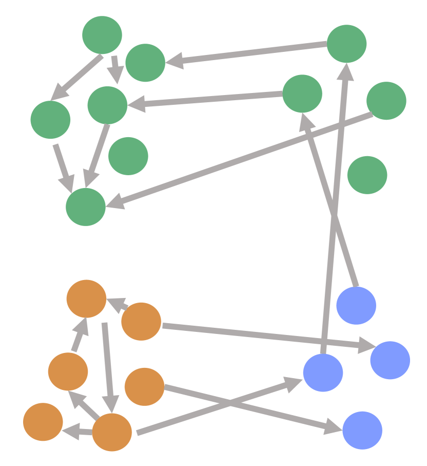
(a)

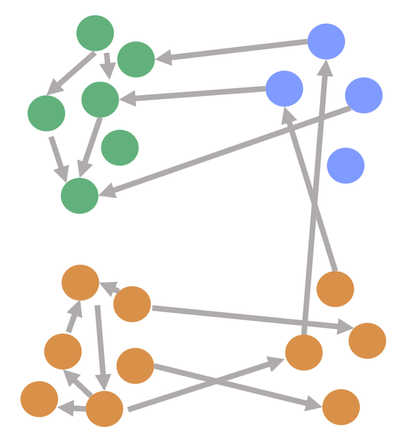
(b)

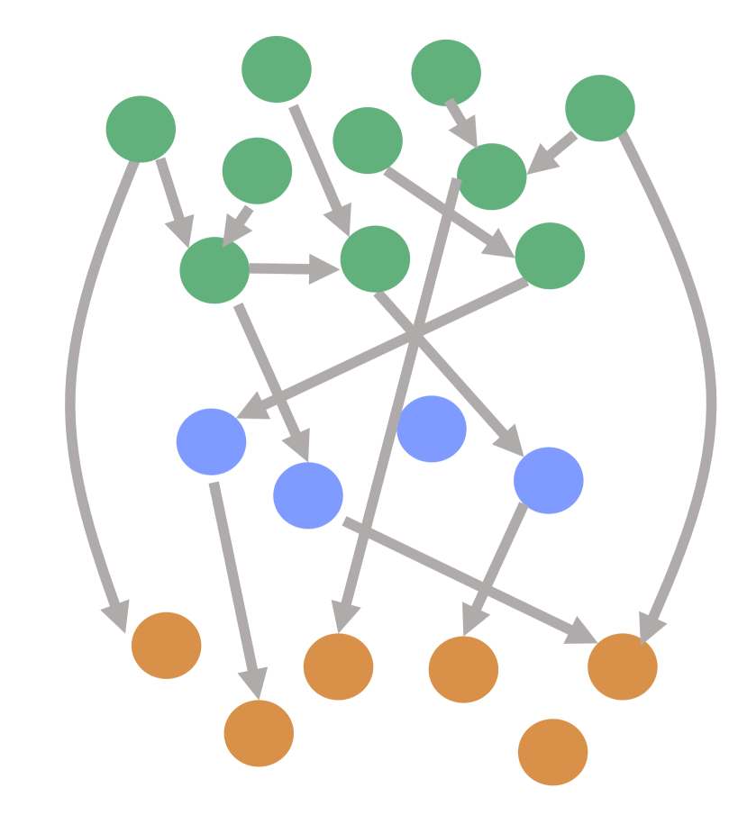
(c)

Figure 1: Illustration for networks under different link probability matrices. Colors indicate communities. (a) row clusters under $B^{(1)}$; (b) column clusters under $B^{(1)}$; (c) Row clusters under $B^{(2)}$ ($B^{(3)}$); column clusters are analogous.

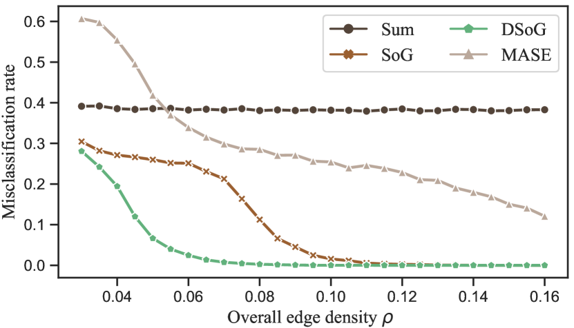
(a) Experiment 1, row clustering

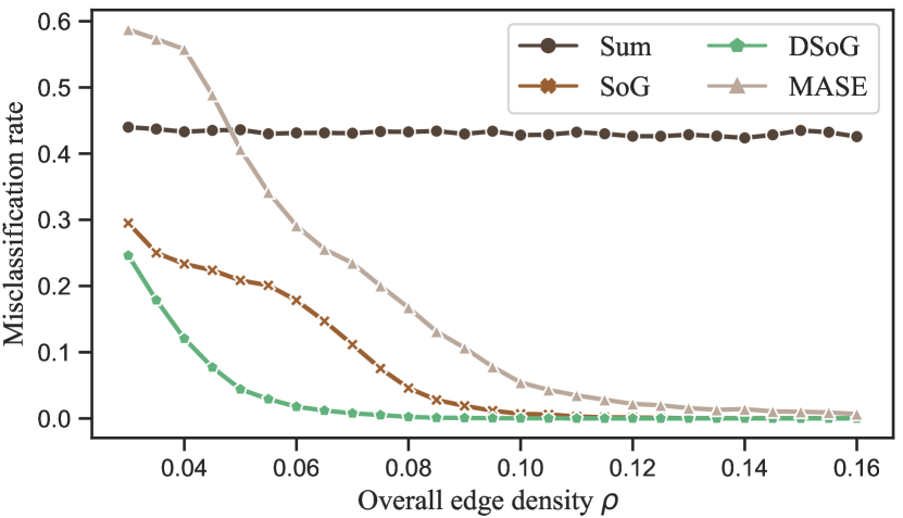
(b) Experiment 1, column clustering

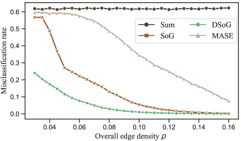
(c) Experiment 2, row clustering

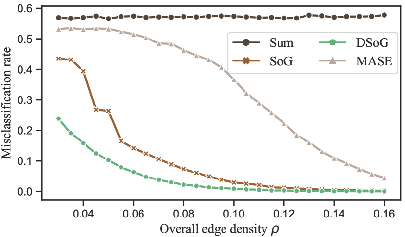
(d) Experiment 2, column clustering

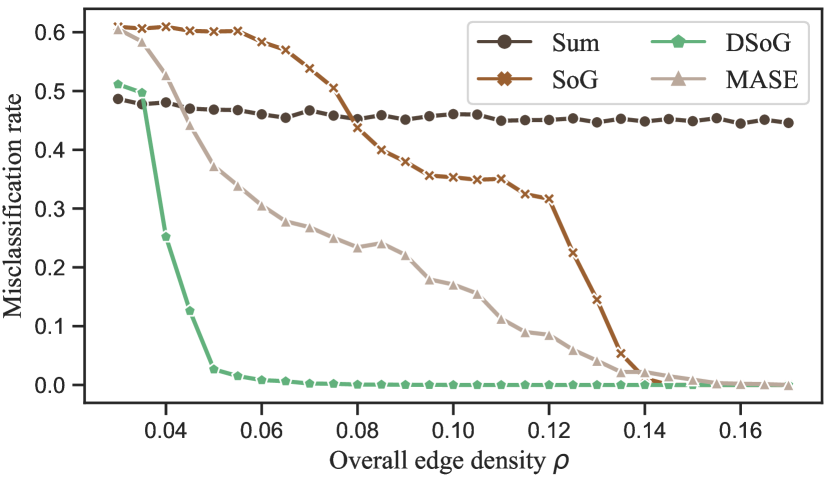
(e) Experiment 3, row clustering

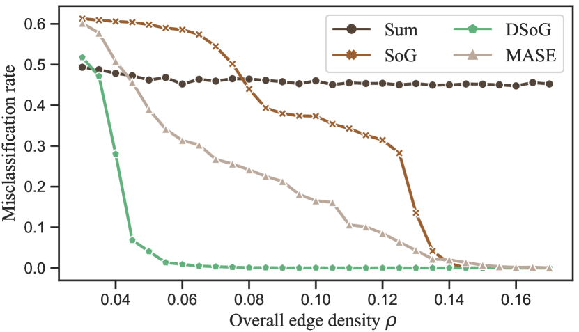
(f) Experiment 3, column clustering

Figure 2: Misclassification rates of four methods with varying $\rho$ in three experimental set-ups. The horizontal directions correspond to Experiments 1-3 sequentially, and the vertical directions correspond to the performance with respect to the row clusters and column clusters, respectively.

Results.

We use the misclassification rate defined in (10) to measure the proportion of misclassified (up to permutations) nodes. The averaged results over 50 replications for Experiments 1-3 are displayed in Figure 2, where we vary $\rho$ from 0.03 to 0.16 in 27 equally-spaced values. The results demonstrate that our proposed method DSoG has a noticeable impact on the accuracy of clustering. Specifically, the Sum method performs poorly due to the fact that some eigen-components cancel out in the summation. The DSoG method has a significant advantage over the SoG method, especially when $\rho$ is small, i.e., the very sparse regime, which is consistent with our theoretical results. We can also observe that our method DSoG outperforms the MASE method in all settings.

5 Real data analysis

In this section, we analyze the WFAT dataset, which is a public dataset collected by the Food and Agriculture Organization of the United Nations. The original data includes trading records for more than 400 food and agricultural products imported/exported annually by all the countries in the world. The dataset is available at https://www.fao.org. As described in other works analyzing these data (De Domenico et al., 2015; Jing et al., 2021; Noroozi and Pensky, 2022), it can be considered as a multi-layer network, where layers represent food and agricultural products, and nodes are countries and edges at each layer represent import/export relationships of a specific food and agricultural product among countries. Jing et al. (2021) and Noroozi and Pensky (2022) partitioned the layers into groups, where the layers within a certain group can be assumed to have networks with common community structures. Thus, we focus on the group obtained by Noroozi and Pensky (2022) to show that our method can produce insightful national communities; see Table 1 for the products we considered.

“Pastry”, “Rice, paddy”, “Rice, milled”, “Breakfast cereals”, Mixes and doughs”,

“Food preparations of flour, meal or malt extract”, “Sugar and syrups n.e.c.”,

“Sugar confectionery”, “Communion wafers and similar products.”, “Prepared nuts”,

“Vegetables preserved (frozen)”, “Juice of fruits n.e.c.”, “Fruit prepared n.e.c.”,

“Orange juice”, “Other non-alcoholic caloric beverages”, “Food wastes”,

“Other spirituous beverages”, “Coffee, decaffeinated or roasted”, “Coffee, green”,

“Chocolate products nes”, “Pepper, raw”, “Dog or cat food, put up for retail sale”,

“Food preparations n.e.c.”, “Crude organic material n.e.c.”

Table 1: List of a group of food and agricultural products obtained by Noroozi and Pensky (2022), which consists of 24 different products involving cereals, stimulant crops, and derived products.

Data preprocessing.

We convert the original trading data into directed networks, which is distinct from all previously described efforts to analyze this data, where the trading data is reduced to an undirected network. We focus on the trading data in year 2020. To create a directed trading network for each of the 24 products, we draw a directed edge from the exporter to the importer if the export/import value of the product exceeds $10000. This particular threshold would yield sparse networks that have many disjoint connected components individually but have one connected component after aggregation. We then removed all the countries (nodes) whose total in-degree or out-degree across all 24 layers is less than 14. We choose this value to make sure that each node has links to at least one of the other nodes in at least half of the layers. Indeed, the average total in-degree and out-degree of nodes which do not have any neighbors in 12 or more of the layers (i.e., more than half of the layers have a zero out-degree or in-degree) is 13. As a result, we obtain a multi-layer network with 24 layers and 142 nodes per layer. Subsequently, we reconstruct the row and column clusters using the proposed algorithm. For this purpose, we choose $K_{y}=5$ and $K_{z}=5$, which is consistent with the number of continents (Asia, Europe, America, Africa and Oceania).

Results.

The estimated row and column clusters are displayed in Figure 3. The clusters of countries are approximately related to their geographic locations, which is coherent with the economic laws of world trade. Specifically, for the row clusters (see Figure 3(a)), Community 1 mainly includes countries in Africa, West, Central and South Asia; Community 2 is composed of countries in Central and South America; Community 3 includes China, the United States, Western and Southern Europe countries; Community 4 involves Southeast Asia and Oceania countries; Community 5 consists of the remaining European countries. For the column clusters (see Figure 3(b)), Community 1 mainly includes Africa and West Asia countries; Community 2 consists of countries in Central and South America; Community 3 includes East and South Asia countries; Community 4 involves Eastern European and some West Asian countries; Community 5 mainly includes Western Europe, North America, Australia and Russia.

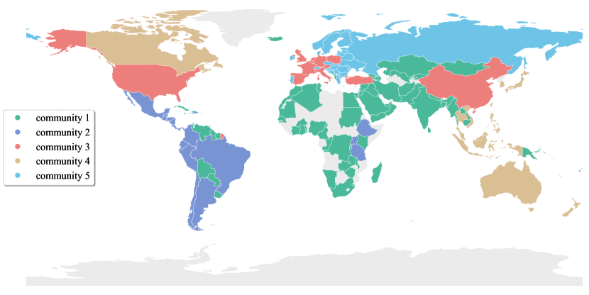
(a) row (export) clustering

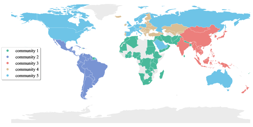
(b) column (import) clustering

Figure 3: Community structure separation of food trade networks (directed) containing 142 major countries. Colors indicate communities, where light gray corresponds to countries that do not participate in clustering.

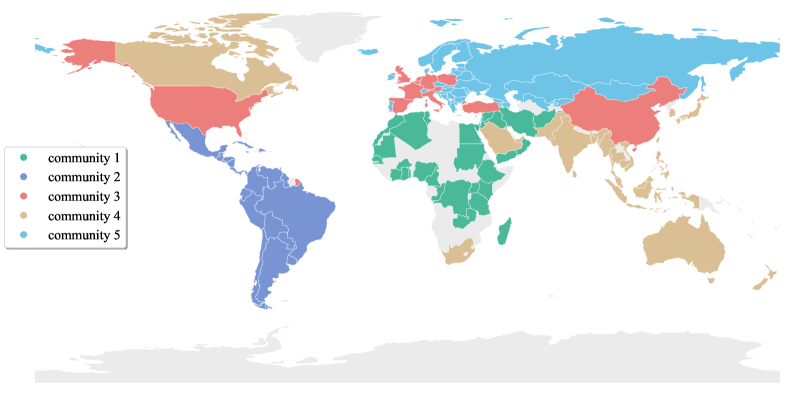
Figure 4: Community structure separation of food trade networks (undirected) containing 142 major countries. Colors indicate communities, where light gray corresponds to countries that do not participate in clustering.

We can see that the structure of the row (export) clusters is not identical to that of the column (import) clusters, which is insightful and more realistic than what would be expected from undirected multi-layer networks. For instance, China is grouped with major European economies and America in the row clusters partition, while it is grouped mainly with East and South Asia countries in the column clusters partition, indicating that for the products in Table 1, China is aligned with major world economies in its export trade, while it is aligned mainly with neighboring countries in its import trade. This observation is entirely plausible. Export patterns primarily reflect a nation’s productive capacity and dominant industries. Major global economies with robust food processing industries and agricultural technology tend to export value-added manufactured goods. Conversely, import patterns primarily mirror a country’s consumer demand. Due to similar geographical conditions, population sizes and food consumption habits, countries in close proximity to each other often exhibit similar import patterns. In contrast, we consider the process of transforming directed graphs into undirected graphs, as mentioned in the introduction, which leads to the clustering results shown in Figure 4. Ignoring the directionality of the edges, the clustering outcome aligns closely with that of the export patterns. This is attributed to the fact that export activities often play a more proactive and decisive role in a nation’s trade patterns. Exports illuminate factors such as a country’s industrial organization, competitiveness, and position in the global value chain. If the export pattern of one country mirrors that of another, they may also show similarities in their overall trade patterns. This could lead to a failure to recognize the unique characteristics of import patterns and thus to a less comprehensive understanding of trade relations.

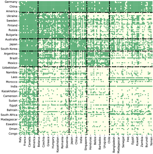
Figure 5: Visualization of the aggregated adjacency matrix. Yellow pixels correspond to the absence of an edge between the corresponding countries while green pixels correspond to an edge. The black dashed lines in the figures signifies the division between clusters.

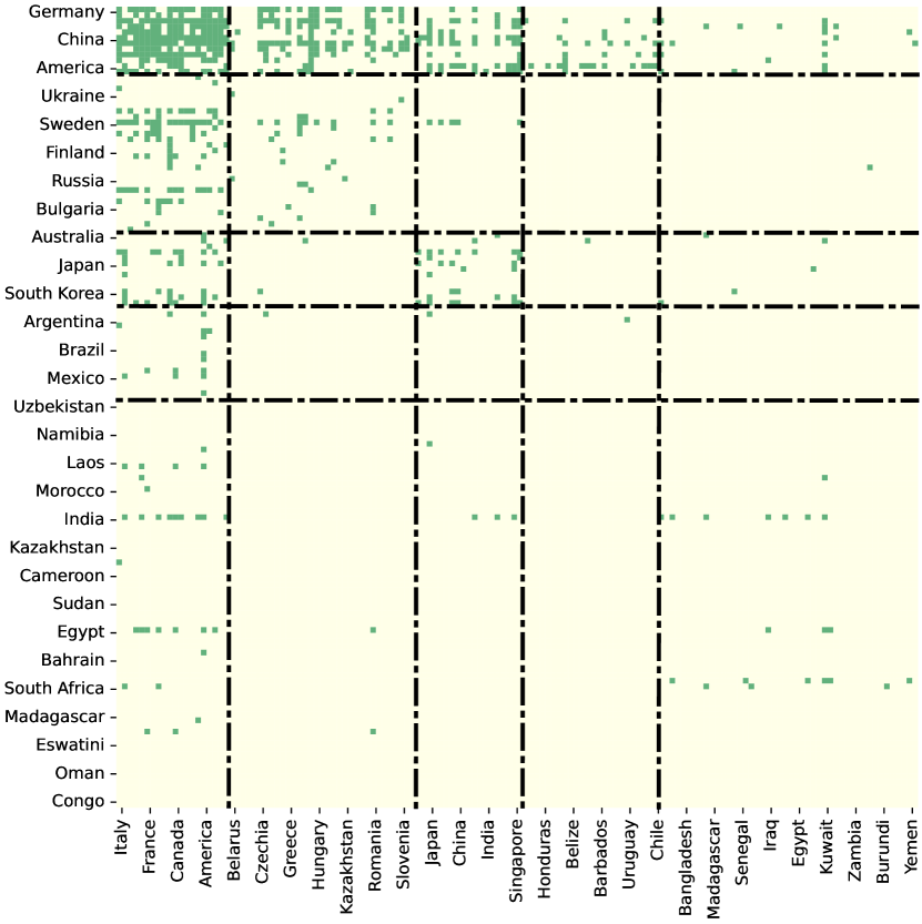
(a) Vegetables preserved (frozen)

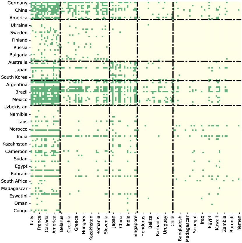
(b) Coffee, green

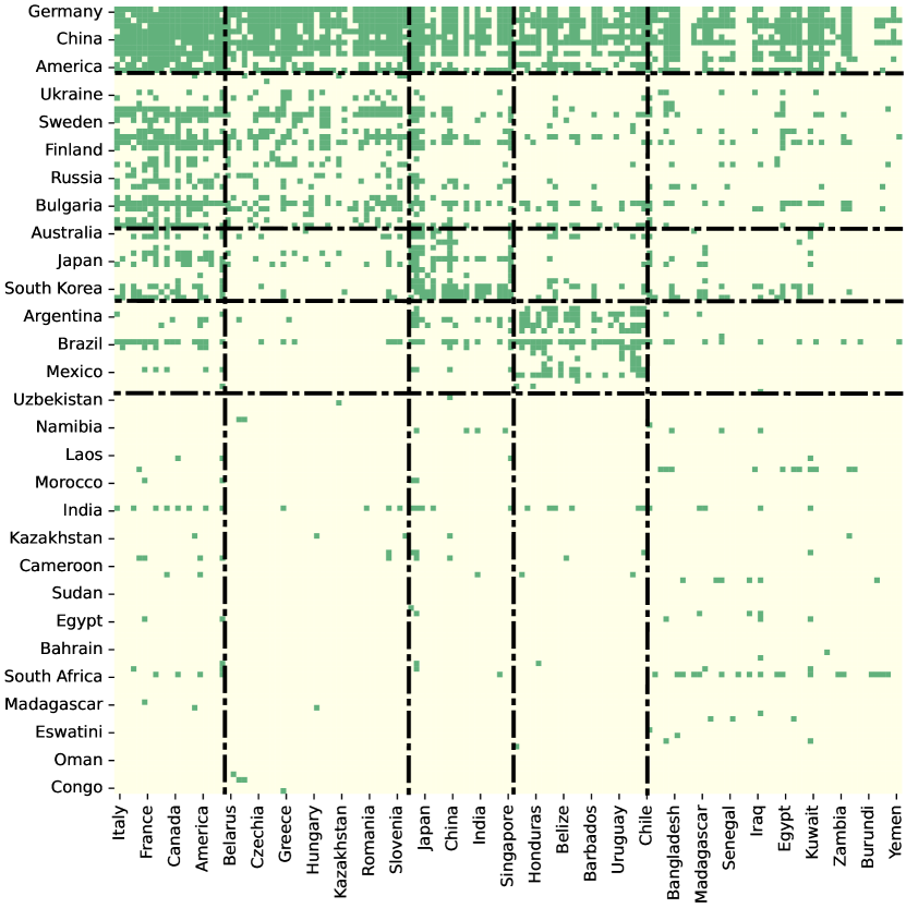
(c) Food wastes

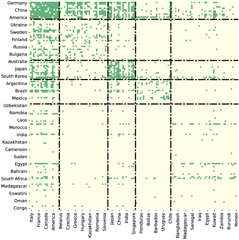
(d) Juice of fruits n.e.c.

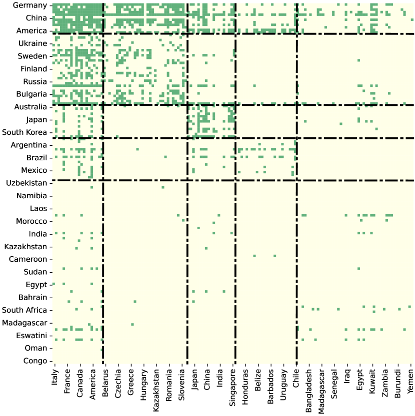
(e) Coffee, decaffeinated or roasted

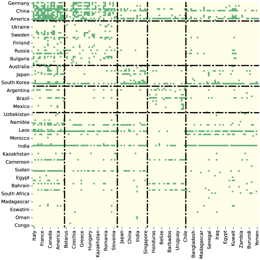
(f) Rice, paddy

Figure 6: Visualization of the adjacency matrices for six products. The colors, node order, and community partition are identical to Figure 5.

Visualizations of the aggregated adjacency matrix and several single-layer adjacency matrices are also presented, which can illustrate the advantages of multi-layer networks and further highlight the difference between sending and receiving patterns. Figure 5 illustrates the network of the products listed in Table 1, aggregated in a summation manner. In Figure 6, the adjacency matrices for the six products featured in Table 1 are displayed. To highlight the clustering outcomes, the order of the nodes (countries) is adjusted accordingly and persists in each plot. Due to space limitations, only a portion of the countries are labeled on the axes. It is clear that our clustering results have a significant community structure, and the row (export) clusters are quite different from the column (import) clusters, as reflected by the fact that the row and column clusters in the same country have distinctly different compositions and different community sizes. Such asymmetric information cannot be captured by undirected networks. More significantly, a comparison between the individual adjacency matrices in Figure 6 and Figure 5 reveals that a single-layer network only encapsulates a fraction of the community structure information, and a more comprehensive picture of trade relations among countries can be obtained by aggregating the individual trade networks for multiple products. This aligns with our original intention of dealing with multi-layer directed networks.

6 Conclusion

In this paper, we studied the problem of detecting co-clusters in multi-layer directed networks. We typically assumed that the multi-layer directed network is generated from the multi-layer ScBM, which allows different row and column clusters via different patterns of sending and receiving edges. The proposed method DSoG is formulated as the spectral co-clustering based on the SoG matrices of the row and column spaces, where a bias correction step is implemented. We systematically studied the algebraic properties of the population version of DSoG. In particular, we did not require that the corresponding link probability matrix be of full rank. We also studied the misclassification error rates of DSoG, which show that under certain condition, multiple layers can bring benefit to the clustering performance. We finally conducted numerical experiments on a number of simulated and real examples to support the theoretical results.

There are many ways to extend the content of this paper. First, we focused on the scenario where the layer-wise community structures are homogeneous. It is of great interest to extend the scenario to associated but inhomogeneous community structures, which has been studied recently for multi-layer undirected networks (Han et al., 2015; Pensky and Zhang, 2019; Chen et al., 2022). Second, we analyzed the WFAT dataset with respect to a particular year. However, this dataset contains the annual trading data from 1986 to the present and is continuously updated, which actually constitutes a higher-order multi-layer network that contains more adequate information than a single multi-layer network. It is thus of great importance to develop a corresponding toolbox for this higher-order multi-layer network. Third, it is important to study the estimation of the number of communities (Fishkind et al., 2013; Ma et al., 2022).

Appendix

Appendix A provides the technical theorem and lemma that are needed to prove the misclassification rates. Appendix B includes the proof of main theorem and lemmas in the main text. Appendix C contains auxiliary lemmas.

A Technical theorem and lemma

Theorem 3.

Let $A_{l}\in\{0,1\}^{n\times n}$ be the adjacency matrices generated by a multi-layer ScBM and $X_{l}=A_{l}-\bar{P}_{l}$ be the asymmetric noise matrices for all $1\leq l\leq L$, where $\bar{P}_{l}=\mathbb{E}(A_{l})$. If $L^{1/2}n\rho\geq c_{1}\log(L+n)$ and $n\rho\leq c_{2}$ for positive constants $c_{1}$ and $c_{2}$, then $E_{1}$, the off-diagonal part of $\sum_{l=1}^{L}X_{l}X_{l}^{T}$, satisfies

$$\|E_{1}\|_{2}\leq cL^{1/2}n\rho\log^{1/2}(L+n)$$

with probability at least $1-O((L+n)^{-1})$ for some constant $c>0$.

To handle the complicated dependence in $E_{1}$ caused by the quadratic form, the key idea in the proof is viewing $E_{1}$ as a matrix-valued U-statistic with a centered kernel function of order two, indexed by the pairs $(i,j)$, and using the decoupling technique described in Lemma 8, which reduces problems on dependent variables to problems on related (conditionally) independent variables. This type of proof technique is also used in Lei and Lin (2022), dealing with the symmetric case. Specifically, rearrange $E_{1}$ as

$$E_{1}=\sum_{l=1}^{L}\sum_{(i,\;j)\neq(i^{\prime},\;j^{\prime})}X_{l,ij}X_{l,i^{\prime}j^{\prime}}e_{i}e_{i^{\prime}}^{T}I_{\{j=j^{\prime}\}},$$ (12)

where $e_{i}$ is the standard basis vector in $\mathbb{R}^{n}$ and pairs ${(i,j),\;(i^{\prime},j^{\prime})}\in\{1,2,\ldots,n\}^{2}$, which can be viewed as a matrix-valued U-statistic defined on the vectors $X_{1,ij},\ldots,X_{L,ij}$ indexed by the pairs $(i,j)$. The decoupling technique reduces the problem of bounding $\|E_{1}\|_{2}$ to that of bounding $\|\sum_{l=1}^{L}X_{l}\widetilde{X}_{l}^{T}\|_{2}$ and $\|\mbox{diag}(\sum_{l=1}^{L}X_{l}\widetilde{X}_{l}^{T})\|_{2}$, where $\widetilde{X}_{l}$ is an independent copy of $X_{l}$ for all $1\leq l\leq L$.

Proof.

To use the decoupling argument, define

$$\widetilde{E}_{1}=\sum_{l=1}^{L}\sum_{(i,\;j)\neq(i^{\prime},\;j^{\prime})}X_{l,ij}\widetilde{X}_{l,i^{\prime}j^{\prime}}e_{i}e_{i^{\prime}}^{T}I_{\{j=j^{\prime}\}},$$

$$\widetilde{E}_{2}=\sum_{l=1}^{L}\sum_{(i,\;j)}X_{l,ij}\widetilde{X}_{l,ij}e_{i}e_{i}^{T},$$

and

$$\widetilde{E}=\sum_{l=1}^{L}X_{l}\widetilde{X}_{l}^{T}=\widetilde{E}_{1}+\widetilde{E}_{2}.$$

where $\widetilde{E}_{1}$ is the zero mean off-diagonal part and $\widetilde{E}_{2}$ is the diagonal part. Note that $\|\widetilde{E}_{1}\|_{2}\leq\|\widetilde{E}\|_{2}+\|\widetilde{E}_{2}\|_{2}$, we control the spectral norm of $\widetilde{E}$ and $\widetilde{E}_{2}$ separately.

First step: Controlling $\widetilde{E}$. Recall that $\widetilde{X}_{l}=\widetilde{A}_{l}-\bar{P}_{l}$, where $\widetilde{A}_{l}$ is an independent copy of $A_{l}$, we reformulate $\widetilde{E}$ as

$$\widetilde{E}=\sum_{l=1}^{L}X_{l}\widetilde{X}_{l}^{T}=\sum_{l=1}^{L}X_{l}\widetilde{A}_{l}^{T}-\sum_{l=1}^{L}X_{l}\bar{P}_{l}^{T}.$$

Applying Lemma 6 with $(v,b)=(2\rho,1)$, if $L^{1/2}n\rho^{1/2}\geq c_{1}\log^{1/2}(L+n)$ for some constant $c_{1}>0$, we have with probability at least $1-O((L+n)^{-1})$ and universal constant $c>0$,

$$\|\sum_{l=1}^{L}X_{l}\bar{P}_{l}^{T}\|_{2}\leq cL^{1/2}n^{3/2}\rho^{3/2}\log^{1/2}(n+L).$$ (13)

Note that the constant $c$ may be different from line to line in this proof.

In order to apply Lemma 6 to control $\sum_{l=1}^{L}X_{l}\widetilde{A}_{l}^{T}$ conditioning on $\widetilde{A}_{1},\ldots,\widetilde{A}_{L}$, we need to upper bound $\max_{l}\|\widetilde{A}_{l}^{T}\|_{2,\infty}$, $\sum_{l=1}^{L}\|\widetilde{A}_{l}^{T}\|_{F}^{2}$ and $\|\sum_{l=1}^{L}\widetilde{A}_{l}\widetilde{A}_{l}^{T}\|_{2}$, respectively. Note that $\widetilde{A}_{l}$ is an independent copy of $A_{l}$, now we bound the corresponding version of $A_{l}$.

We first consider $\max_{l}\|A_{l}^{T}\|_{2,\infty}$. Note that $\mathbb{E}d_{l,i}^{in}\leq n\rho$. Applying a union bound over $i\in[n]$ and $l\in[L]$, along with the standard Bernstein’s inequality

$$\mathbb{P}(d_{l,i}^{in}-\mathbb{E}d_{l,i}^{in}\geq t)\leq\exp\left(-\frac{t^{2}/2}{n\rho+t}\right)$$

for all $t>0$, and using the assumption that $n\rho\leq c_{2}$, then with probability at least $1-O((L+n)^{-1})$, we have

$$\max_{l}\|A_{l}^{T}\|_{2,\infty}=\max_{l,i}\sqrt{d_{l,i}^{in}}\leq c\log^{1/2}(L+n).$$ (14)

For $\sum_{l=1}^{L}\|A_{l}^{T}\|_{F}^{2}$, using Bernstein’s inequality for $\sum_{l=1}^{L}d_{l,i}^{in}$ and the assumption that $L^{1/2}n\rho\geq c_{1}\log(L+n)$, we have with probability at least $1-O((L+n)^{-1})$,

$$\sum_{l=1}^{L}\|A_{l}^{T}\|_{F}^{2}\leq n\max_{i}\sum_{l=1}^{L}d_{l,i}^{in}\leq cLn^{2}\rho.$$ (15)

Now we turn to $\|\sum_{l=1}^{L}A_{l}A_{l}^{T}\|_{2}$. To begin with, decompose $\sum_{l=1}^{L}A_{l}A_{l}^{T}$ as $F_{1}+F_{2}$, where $F_{1}$ is the off-diagonal part, which can be viewed as a matrix-valued U-statistic as in (12), and $F_{2}$ is the diagonal part. For the off-diagonal part $F_{1}$, $\widetilde{F}_{1}$ is defined as the off-diagonal part of $\sum_{l=1}^{L}A_{l}\widetilde{A}_{l}^{T}$ for the purpose of using the decoupling technique. Using symmetrization and Perron-Frobenius theorem, we have

$$\|\widetilde{F}_{1}\|_{2}=\begin{Vmatrix}0&\widetilde{F}_{1}\\ \widetilde{F}_{1}^{T}&0\end{Vmatrix}_{2}\leq\max\left\{\|\widetilde{F}_{1}\|_{1,\infty},\|\widetilde{F}_{1}^{T}\|_{1,\infty}\right\}\leq\max\left\{\left\|\sum_{l=1}^{L}A_{l}\widetilde{A}_{l}^{T}\right\|_{1,\infty},\left\|\sum_{l=1}^{L}\widetilde{A}_{l}A_{l}^{T}\right\|_{1,\infty}\right\}.$$

By simple calculations, the $l_{1}$ norm of the $i$th row of $\sum_{l=1}^{L}A_{l}\widetilde{A}_{l}^{T}$ is $\sum_{l=1}^{L}\sum_{j=1}^{n}A_{l,ij}\widetilde{d}_{l,j}^{in}$. Combining (14) and (15) with Bernstein’s inequality, we have

$$\mathbb{P}\left(\left.\sum_{l=1}^{L}\sum_{j=1}^{n}A_{l,ij}\widetilde{d}_{l,j}^{in}-\sum_{l=1}^{L}\sum_{j=1}^{n}\mathbb{E}(A_{l,ij})\widetilde{d}_{l,j}^{in}\geq t\right|\widetilde{A}_{1},\ldots,\widetilde{A}_{L}\right)$$

$$\leq \exp\left(-\frac{t^{2}/2}{cLn^{2}\rho^{2}\log(L+n)+c\log(L+n)t}\right)$$

for all $t>0$. By applying the total probability theorem, the union bound, and the assumption that $L^{1/2}n\rho\geq c_{1}\log(L+n)$, we have with high probability, $\max_{i}\sum_{l=1}^{L}\sum_{j=1}^{n}A_{l,ij}\widetilde{d}_{l,j}^{in}\leq cL^{1/2}n\rho\log(L+n)\leq cLn^{2}\rho^{2}$. A similar argument is conducted for $\sum_{l=1}^{L}\widetilde{A}_{l}A_{l}^{T}$. By Lemma 8 we have

$$\|F_{1}\|_{2}\leq cLn^{2}\rho^{2}$$ (16)

with high probability. For the diagonal part $F_{2}$, applying (15), we have

$$\|F_{2}\|_{2}=\max_{i}\sum_{l=1}^{L}d_{l,i}^{out}\leq cLn\rho$$ (17)

with high probability. Combining (16), (17) with the assumption that $n\rho\leq c_{2}$, we have with probability at least $1-O((L+n)^{-1})$,

$$\left\|\sum_{l=1}^{L}A_{l}A_{l}^{T}\right\|_{2}\leq cLn\rho.$$

So combining the bounds for $\max_{l}\|\widetilde{A}_{l}^{T}\|_{2,\infty}$, $\sum_{l=1}^{L}\|\widetilde{A}_{l}^{T}\|_{F}^{2}$ and $\|\sum_{l=1}^{L}\widetilde{A}_{l}\widetilde{A}_{l}^{T}\|_{2}$, and applying Lemma 6, we have with probability at least $1-O((L+n)^{-1})$,

$$\left\|\sum_{l=1}^{L}X_{l}\widetilde{A}_{l}^{T}\right\|_{2}\leq cL^{1/2}n\rho\log^{1/2}(L+n).$$

Combining this with (13), we have with probability at least $1-O((L+n)^{-1})$,

$$\|\widetilde{E}\|_{2}\leq cL^{1/2}n\rho\log^{1/2}(L+n).$$

Second step: Controlling $\widetilde{E}_{2}$. Recall that $\widetilde{E}_{2}$ is a diagonal matrix whose $i$th diagonal element is $\sum_{l=1}^{L}\sum_{j=1}^{n}X_{l,ij}\widetilde{X}_{l,ij}$. Using standard Bernstein’s inequality and union bound, we have with probability at least $1-O((L+n)^{-1})$,

$$\|\widetilde{E}_{2}\|_{2}\leq cL^{1/2}n\rho\log^{1/2}(L+n).$$

The claim follows by combining the bounds for $\|\widetilde{E}\|_{2}$ and $\|\widetilde{E}_{2}\|_{2}$ together with the decoupling inequality in Lemma 8. ∎

Lemma 5.

Let $H$ be an $n\times s$ matrix with full column rank and the $s$th eigenvalue of $HH^{T}$ is at least $h$ for some constant $h>0$. Let $G$ be an $s\times s$ symmetric matrix with ${\rm rank}(G)=j\leq s$ and the $j$th eigenvalue of $G$ is at least $g$ for some constant $g>0$. Then $\lambda_{j}(HGH^{T})\geq hg$.

Proof.

Note that $\mbox{rank}(H)=s$, we have $\mbox{dim}\{x\in\mathbb{R}^{n}\leavevmode\nobreak\ |\leavevmode\nobreak\ x\perp\mbox{null}(H^{T})\}=s$, where $\mbox{null}(H^{T})$ is the nullspace of $H^{T}$ and is given by $\mbox{null}(H^{T}):=\{\theta\in\mathbb{R}^{n}\leavevmode\nobreak\ |\leavevmode\nobreak\ H^{T}\theta=0\}$. Combining this with $\mbox{rank}(G)=j$, we have $\mbox{dim}\{x\in\mathbb{R}^{n}\leavevmode\nobreak\ |\leavevmode\nobreak\ x\perp\mbox{null}(H^{T}),\;H^{T}x\perp\mbox{null}(G)\}=s$. Thus

$$\min_{x\in\mathbb{R}^{n},\;x\perp\mbox{null}(H^{T}),\;H^{T}x\perp\mbox{null}(G)}\frac{x^{T}HGH^{T}x}{x^{T}x}\geq g\cdot\min_{x\in\mathbb{R}^{n},\;x\perp\mbox{null}(H^{T})}\frac{x^{T}HH^{T}x}{x^{T}x}\geq hg.$$

Applying the Courant-Fischer minimax theorem (Theorem 8.1.2 of Golub and Van Loan (2013)), intersecting on this event, we have

$$\lambda_{j}(HGH^{T})=\max_{\mbox{dim}(\mathscr{H})=j}\min_{0\neq x\in\mathscr{H}}\frac{x^{T}HGH^{T}x}{x^{T}x}\geq hg,$$

where $\mathscr{H}$ is the subspace of $\mathbb{R}^{n}$. The proof is completed. ∎

B Main proofs

Proof of Theorem 1

We decompose the matrix $S^{R}$ into the sum of a signal term and noise terms.

Recall that $\mathcal{P}_{l}=\rho YB_{l}Z^{T}$ and $\bar{P}_{l}=\mathcal{P}_{l}-\mbox{diag}(\mathcal{P}_{l})$. Define

$$N_{4}=\mbox{diag}(\sum_{l=1}^{L}X_{l}X_{l}^{T})-\sum_{l=1}^{L}D_{l}^{out}$$

and recall the definition of $S^{R}$ in (8) and the decomposition (5), we have

$$S^{R}=\sum_{l=1}^{L}\mathcal{P}_{l}\mathcal{P}_{l}^{T}+N_{1}+N_{2}+N_{3}+N_{4}.$$

We first control the signal term. Recall that $\Delta_{z}=\mbox{diag}(\sqrt{n_{1}^{z}},\ldots,\sqrt{n_{K_{z}}^{z}})$ is a $K_{z}\times K_{z}$ diagonal matrix, then $Z=\widetilde{Z}\Delta_{z}$ with $\widetilde{Z}$ being a column orthogonal matrix. By the balanced community sizes assumption and the number of column clusters $K_{z}$ is fixed, the minimum eigenvalue of $\Delta_{z}$ is lower bounded by $c_{0}n^{1/2}$ for some constant $c_{0}>1$. Then we have

$$\sum_{l=1}^{L}\mathcal{P}_{l}\mathcal{P}_{l}^{T}=\rho^{2}\sum_{l=1}^{L}YB_{l}\Delta_{z}\widetilde{Z}^{T}\widetilde{Z}\Delta_{z}B_{l}^{T}Y^{T}\succeq c_{0}n\rho^{2}Y\left[\sum_{l=1}^{L}B_{l}B_{l}^{T}\right]Y^{T},$$

where $\succeq$ denotes the Loewner partial order, in particular, let $A$ and $B$ be two Hermitian matrices of order $p$, we say that $A\succeq B$ if $A-B$ is positive semi-definite. Note that $Y$ is of full column rank and the $K_{y}$th (and smallest) non-zero eigenvalue of $YY^{T}$ is lower bounded by $c_{0}n$ for some constant $c_{0}$, where we used the balanced community sizes assumption and the number of row clusters $K_{y}$ is fixed. Using Lemma 5 and Assumption 2, we can lower bound the $K$th eigenvalue of $\sum_{l=1}^{L}\mathcal{P}_{l}\mathcal{P}_{l}^{T}$ to be

$$\lambda_{K}(\sum_{l=1}^{L}\mathcal{P}_{l}\mathcal{P}_{l}^{T})\geq cLn^{2}\rho^{2}$$

for some constant $c>0$. Note that we use $c_{0}$, $c_{1}$, $c_{2}$ and $c$ to represent the generic constants and they may be different from line to line.

Then we bound each noise term respectively. The first noise term $N_{1}$ is non-random and satisfies

$$\|N_{1}\|_{2}\leq n\|N_{1}\|_{\max}\leq Ln\rho^{2}.$$

For $N_{2}$, recalling that $X_{l}=A_{l}-\bar{P}_{l}$, where $X_{l,ij}(1\leq i,j\leq n)$ is generated independently from centered Bernoulli, and is therefore $(2\rho,1)$-Bernstein. Using Lemma 6 and the fact that $\|\bar{P}_{l}^{T}\bar{P}_{l}\|_{2}\leq n^{2}\rho^{2}$, $\|\bar{P}_{l}\|_{2}\leq n^{2}\rho^{2}$ and $\|\bar{P}_{l}\|_{2,\infty}\leq n^{1/2}\rho$, if $L^{1/2}n\rho^{1/2}\geq c_{1}\log^{1/2}(L+n)$ for some constant $c_{1}>0$, we have with probability at least $1-O((L+n)^{-1})$ and universal constant $c>0$,

$$\|N_{2}\|_{2}\leq cL^{1/2}n^{3/2}\rho^{3/2}\log^{1/2}(n+L).$$

For the noise term $N_{3}$, applying Theorem 3, we have

$$\|N_{3}\|_{2}\leq cL^{1/2}n\rho\log^{1//2}(L+n)$$

with probability at least $1-O((L+n)^{-1})$.

We next control $N_{4}$. The construction in (7) implies that

$$\|N_{4}\|_{2}\leq Ln\rho^{2}.$$

Let $U$ and $\widehat{U}$ be the $n\times K$ matrices consisting of the leading eigenvectors of $\sum_{l=1}^{L}\mathcal{P}_{l}\mathcal{P}_{l}^{T}$ and $S^{R}$, respectively. We are now ready to bound the derivation of $\widehat{U}$ from $U$. Combining the lower bound of signal term and upper bound of all noise terms, we have with high probability,

$$\frac{\|N_{1}+N_{2}+N_{3}+N_{4}\|_{2}}{\lambda_{K}(\sum_{l=1}^{L}\mathcal{P}_{l}\mathcal{P}_{l}^{T})} \leq c\ \frac{Ln\rho^{2}+L^{1/2}n\rho\log^{1/2}(L+n)}{Ln^{2}\rho^{2}}$$

$$\leq \frac{c}{n}+\frac{c\log^{1/2}(L+n)}{L^{1/2}n\rho},$$

where the first inequality arises from the merging of the $N_{2}$ and $N_{3}$ terms when $n\rho\leq c_{2}$ for some constant $c_{2}>0$. By Proposition 2.2 of Vu and Lei (2013) and Davis-Kahan sin$\Theta$ theorem (Theorem VII.3.1 of Bhatia (1997)), there exists a $K\times K$ orthogonal matrix $O$ such that

$$\|\widehat{U}-UO\|_{F} \leq \sqrt{K}\|\widehat{U}-UO\|_{2}$$

$$\leq \frac{\sqrt{K}\|N_{1}+N_{2}+N_{3}+N_{4}\|_{2}}{\lambda_{K}(\sum_{l=1}^{L}\mathcal{P}_{l}\mathcal{P}_{l}^{T})-\|N_{1}+N_{2}+N_{3}+N_{4}\|_{2}}$$

$$\lesssim \frac{1}{n}+\frac{\log^{1/2}(L+n)}{L^{1/2}n\rho},$$

where $a_{n}\lesssim b_{n}$ means that there exists some positive constant $c$ such that $a_{n}\leq cb_{n}$ for all $n$. Finally, by using Lemma 7, we are able to obtain the desired bound for the misclassification rate.

Proof of Lemma 1

Define $\Delta_{y}=\mbox{diag}(\sqrt{n_{1}^{y}},\ldots,\sqrt{n_{K_{y}}^{y}})$ as a $K_{y}\times K_{y}$ diagonal matrix with $k$th diagonal entry being the $l_{2}$ norm of the $k$th column of $Y$. Then $Y\Delta_{y}^{-1}$ is a column orthogonal matrix. Similarly define $\Delta_{z}={\rm diag}(\sqrt{n_{1}^{z}},\ldots,\sqrt{n_{K_{z}}^{z}})$. Write $\mathcal{P}^{R}$ as

$$\mathcal{P}^{R} = \rho^{2}Y\sum_{l=1}^{L}B_{l}Z^{T}ZB_{l}^{T}Y^{T}$$

$$= \rho^{2}Y\Delta_{y}^{-1}\Delta_{y}\sum_{l=1}^{L}B_{l}\Delta_{z}^{2}B_{l}^{T}\Delta_{y}\Delta_{y}^{-1}Y^{T}=\rho^{2}Y\Delta_{y}^{-1}Q^{R}D^{R}{Q^{R}}^{T}\Delta_{y}^{-1}Y^{T},$$

where we used the eigen-decomposition of $\Delta_{y}\sum_{l=1}^{L}B_{l}\Delta_{z}^{2}B_{l}^{T}\Delta_{y}$ is $Q^{R}D^{R}{Q^{R}}^{T}$. Here $Q^{R}$ is a $K_{y}\times K$ column orthogonal matrix and $D^{R}$ is a $K\times K$ diagonal matrix, which is due to the fact that $Z^{T}Z$ is a positive definite diagonal matrix, and hence the rank of $\sum_{l=1}^{L}B_{l}B_{l}^{T}$ is equal to the rank of $\Delta_{y}\sum_{l=1}^{L}B_{l}\Delta_{z}^{2}B_{l}^{T}\Delta_{y}$.

It is easy to see that $Y\Delta_{y}^{-1}Q^{R}$ has orthogonal columns, so we have

$$U=Y\Delta_{y}^{-1}Q^{R}.$$ (18)

When $\sum_{l=1}^{L}B_{l}B_{l}^{T}$ is of full rank, that is, $K=K_{y}$, $\Delta_{y}^{-1}Q^{R}$ is invertible, thus $Y_{i\ast}=Y_{j\ast}$ if and only if $U_{i\ast}=U_{j\ast}$. The first claim follows by the fact that the rows of $\Delta_{y}^{-1}Q^{R}$ are perpendicular to each other and the $k$th row has length $\sqrt{n_{k}^{y}}$.

When $\sum_{l=1}^{L}B_{l}B_{l}^{T}$ is rank-deficient, that is, $K<K_{y}$, $Y_{i\ast}=Y_{j\ast}$ can also imply $U_{i\ast}=U_{j\ast}$ by (18). On the other hand, by (18), $\|U_{i\ast}-U_{j\ast}\|_{2}:=\|\frac{Q^{R}_{g_{i}^{y}\ast}}{\sqrt{n_{g_{i}^{y}}}}-\frac{Q^{R}_{g_{j}^{y}\ast}}{\sqrt{n_{g_{j}^{y}}}}\|_{2}$. The second claim follows by the rows of $\Delta_{y}^{-1}Q^{R}$ are mutually distinct with their minimum Euclidean distance being larger than a deterministic sequence $\{\zeta_{n}\}_{n\geq 1}$. $\hfill\qed$

Proof of Lemma 2

By the balanced community sizes assumption and both $K_{y}$ and $K_{z}$ are fixed, we have

$$\Delta_{y}\sum_{l=1}^{L}B_{l}\Delta_{z}^{2}B_{l}^{T}\Delta_{y}\preceq c_{1}n\Delta_{y}\sum_{l=1}^{L}B_{l}B_{l}^{T}\Delta_{y}\preceq c_{1}Ln\Delta_{y}^{2}\preceq c_{1}Ln^{2}I_{K_{y}},$$ (19)

where we used $\Delta_{z}^{2}\preceq\frac{c_{0}n}{K_{z}}I_{K_{z}}$, $\Delta_{y}^{2}\preceq\frac{c_{0}n}{K_{y}}I_{K_{y}}$ and $\|\sum_{l=1}^{L}B_{l}B_{l}^{T}\|_{2}\leq LK_{y}^{2}$. Recall that the eigen-decomposition of $\Delta_{y}\sum_{l=1}^{L}B_{l}\Delta_{z}^{2}B_{l}^{T}\Delta_{y}$ is $Q^{R}D^{R}{Q^{R}}^{T}$, (19) implies that $D^{R}_{ii}$ is upper bounded by $c_{1}Ln^{2}$ for any $1\leq i\leq K$. Note that we use $c_{1}$ and $c_{2}$ to represent the generic positive constants and they may be different from line to line.

Define $\mathbb{B}^{R}:=\sum_{l=1}^{L}B_{l}\Delta_{z}^{2}B_{l}^{T}$, by simple calculations, we have

$$\mathbb{B}^{R}_{g_{i}^{y}g_{j}^{y}}=\sum_{k_{z}=1}^{K_{z}}\sum_{l=1}^{L}n_{k_{z}}^{z}B_{l,g_{i}^{y}k_{z}}B_{l,g_{j}^{y}k_{z}}$$

for all $1\leq i,j\leq n$. Under the Assumption 1, it is easy to see that

$$\mathbb{B}^{R}_{g_{i}^{y}g_{j}^{y}}\geq\frac{n}{c_{0}K_{z}}\left[\sum_{l=1}^{L}B_{l}B_{l}^{T}\right]_{g_{i}^{y}g_{j}^{y}}$$

and

$$\mathbb{B}^{R}_{g_{i}^{y}g_{j}^{y}}\leq\frac{c_{0}n}{K_{z}}\left[\sum_{l=1}^{L}B_{l}B_{l}^{T}\right]_{g_{i}^{y}g_{j}^{y}}.$$

Let $\mu^{r}_{n}:=c_{1}Ln^{2}$, by the decomposition (18), we have

$$\mu^{r}_{n}\|U_{i\ast}-U_{j\ast}\|_{2}^{2} = \sum_{k=1}^{K}\mu^{r}_{n}(\frac{Q^{R}_{g_{i}^{y}k}}{\sqrt{n_{g_{i}^{y}}}}-\frac{Q^{R}_{g_{j}^{y}k}}{\sqrt{n_{g_{j}^{y}}}})^{2}$$

$$\geq \sum_{k=1}^{K}D^{R}_{kk}(\frac{Q^{R}_{g_{i}^{y}k}}{\sqrt{n_{g_{i}^{y}}}}-\frac{Q^{R}_{g_{j}^{y}k}}{\sqrt{n_{g_{j}^{y}}}})^{2}$$

$$= \sum_{k=1}^{K}D^{R}_{kk}(\frac{Q^{R}_{g_{i}^{y}k}}{\sqrt{n_{g_{i}^{y}}}})^{2}+\sum_{k=1}^{K}D^{R}_{kk}(\frac{Q^{R}_{g_{j}^{y}k}}{\sqrt{n_{g_{j}^{y}}}})^{2}-2\sum_{k=1}^{K}D^{R}_{kk}\frac{Q^{R}_{g_{i}^{y}k}Q^{R}_{g_{j}^{y}k}}{\sqrt{n_{g_{i}^{y}}n_{g_{j}^{y}}}}$$

$$= \mathbb{B}^{R}_{g_{i}^{y}g_{i}^{y}}+\mathbb{B}^{R}_{g_{j}^{y}g_{j}^{y}}-2\mathbb{B}^{R}_{g_{i}^{y}g_{j}^{y}}$$

$$\geq \frac{n}{c_{0}K_{z}}\left[\sum_{l=1}^{L}B_{l}B_{l}^{T}\right]_{g_{i}^{y}g_{i}^{y}}+\frac{n}{c_{0}K_{z}}\left[\sum_{l=1}^{L}B_{l}B_{l}^{T}\right]_{g_{j}^{y}g_{j}^{y}}-2\frac{c_{0}n}{K_{z}}\left[\sum_{l=1}^{L}B_{l}B_{l}^{T}\right]_{g_{i}^{y}g_{j}^{y}}$$

$$\geq c_{1}nL\eta^{r}_{n}$$

for some constant $c_{1}>0$, where the last inequality is implied by our condition, since $\sum_{l=1}^{L}B_{l}B_{l}^{T}=B^{R}(B^{R})^{T}$, the $g_{i}^{y}g_{j}^{y}$-th element of $\sum_{l=1}^{L}B_{l}B_{l}^{T}$ is the inner product of $B^{R}_{g_{i}^{y}\ast}$ and $B^{R}_{g_{j}^{y}\ast}$. As a result, for any $Y_{i\ast}\neq Y_{j\ast}$, we have $\|U_{i\ast}-U_{j\ast}\|_{2}\geq c_{2}\sqrt{\eta^{r}_{n}/n}$ for some constant $c_{2}>0$. $\hfill\qed$

Proof of Lemma 3

By the fact that the rank of $\sum_{l=1}^{L}B_{l}^{T}B_{l}$ is equal to the rank of $\Delta_{z}\sum_{l=1}^{L}B_{l}^{T}\Delta_{y}^{2}B_{l}\Delta_{z}$, we have $Q^{C}$ is a $K_{z}\times K$ column orthogonal matrix. It is easy to see that $Z\Delta_{z}^{-1}Q^{C}$ has orthogonal columns, so we have

$$V=Z\Delta_{z}^{-1}Q^{C}.$$

The rest proof is similar to that of Lemma 1, we omit it here. $\hfill\qed$

Proof of Lemma 4

The proof of Lemma 4 follows the same strategy as that of Lemma 2. Here we only describe the difference.

Define $\mu^{c}_{n}:=c_{1}Ln^{2}$ and $\mathbb{B}^{C}:=\sum_{l=1}^{L}B_{l}^{T}\Delta_{y}^{2}B_{l}$, by simple calculations, we have

$$\mathbb{B}^{C}_{g_{i}^{z}g_{j}^{z}}=\sum_{k_{y}=1}^{K_{y}}\sum_{l=1}^{L}n_{k_{y}}^{z}B_{l,k_{y}g_{i}^{z}}B_{l,k_{y}g_{j}^{z}}$$

for all $1\leq i,j\leq n$. Combining this with Assumption 1 and $V=Z\Delta_{z}^{-1}Q^{C}$, we have

$$\mu^{c}_{n}\|V_{i\ast}-V_{j\ast}\|_{2}^{2} \geq \sum_{k=1}^{K^{\prime}}D^{C}_{kk}(\frac{Q^{C}_{g_{i}^{z}k}}{\sqrt{n_{g_{i}^{z}}}}-\frac{Q^{C}_{g_{j}^{z}k}}{\sqrt{n_{g_{j}^{z}}}})^{2}$$

$$= \mathbb{B}^{C}_{g_{i}^{z}g_{i}^{z}}+\mathbb{B}^{C}_{g_{j}^{z}g_{j}^{z}}-2\mathbb{B}^{C}_{g_{i}^{z}g_{j}^{z}}$$

$$\geq \frac{n}{c_{0}K_{y}}\left[\sum_{l=1}^{L}B_{l}^{T}B_{l}\right]_{g_{i}^{z}g_{i}^{z}}+\frac{n}{c_{0}K_{y}}\left[\sum_{l=1}^{L}B_{l}^{T}B_{l}\right]_{g_{j}^{z}g_{j}^{z}}-2\frac{c_{0}n}{K_{y}}\left[\sum_{l=1}^{L}B_{l}^{T}B_{l}\right]_{g_{i}^{z}g_{j}^{z}}$$

$$\geq c_{1}nL\eta^{c}_{n}$$

for some constant $c_{1}>0$, where the last inequality is implied by our condition, since $\sum_{l=1}^{L}B_{l}^{T}B_{l}=B^{C}(B^{C})^{T}$, the $g_{i}^{z}g_{j}^{z}$-th element of $\sum_{l=1}^{L}B_{l}^{T}B_{l}$ is the inner product of $B^{C}_{g_{i}^{z}\ast}$ and $B^{C}_{g_{j}^{z}\ast}$. As a result, for any $Z_{i\ast}\neq Z_{j\ast}$, we have $\|V_{i\ast}-V_{j\ast}\|_{2}\geq c_{2}\sqrt{\eta^{c}_{n}/n}$ for some constant $c_{2}>0$. $\hfill\qed$

C Auxiliary lemmas

Given a random variable $X$, we say that Bernstein’s condition with parameters $v$ and $b$ holds if $\mathbb{E}[|X|^{k}]\leq\frac{v}{2}k!b^{k-2}$ for all integers $k\geq 2$. It is also said that $X$ is $(v,b)$-Bernstein.

Lemma 6 (Theorem 3 in Lei and Lin (2022)).

For $1\leq l\leq L$, let $W_{l}$ be a sequence of independent $n\times n$ matrices with zero mean independent entries, and $H_{l}$ be any sequence of $n\times n$ non-random matrices. If for all $1\leq l\leq L$ and $1\leq i,j\leq n$, each entry $W_{l,ij}$ is $(v,b)$-Bernstein, then for all $t>0$,

$$\mathbb{P}\left(\|\sum_{l=1}^{L}W_{l}H_{l}\|_{2}\geq t\right)\leq 4n\exp\left(-\frac{t^{2}/2}{v\max(n\|\sum_{l=1}^{L}H_{l}^{T}H_{l}\|_{2},\;\sum_{l=1}^{L}\|H_{l}\|_{F}^{2})+b\max_{l}\|H_{l}\|_{2,\infty}t}\right).$$

Lemma 7 (Lemma 5.3 in Lei and Rinaldo (2015)).

Let $U$ be an $n\times d$ matrix with $K$ distinct rows with minimum pairwise Euclidean norm separation $\gamma>0$. Let $\widehat{U}$ be another $n\times d$ matrix and $(\widehat{\Theta},\widehat{X})$ be an solution to $k$-means problem with input $\widehat{U}$, then the number of errors in $\widehat{\Theta}$ as an estimate of the row clusters of $U$ is no larger than $c\|\widehat{U}-U\|_{F}^{2}\gamma^{-2}$ for some constant $c>0$.

Lemma 8 (Theorem 1 in de la Peña and Montgomery-Smith (1995)).

Let $\{X_{i}\}_{i=1}^{n}$ be a sequence of independent random variables in a measurable space $(\mathcal{S},\mathscr{S})$, and let $\{X_{i}^{(j)}\}$, $j=1,\ldots,k$ be $k$ independent copies of $\{X_{i}\}$. Let $f_{i_{1}i_{2}\ldots i_{k}}$ be families of functions of $k$ variables taking $(\mathcal{S}\times\ldots\mathcal{S})$ into a Banach space $(\mathcal{B},\|\cdot\|)$. Then, for all $n\geq k\geq 2,\;t>0$, there exist numerical constant $c_{k}>0$ depending on $k$ only so that,

$$\mathbb{P}(\|\sum_{1\leq i_{1}\neq i_{2}\neq\ldots\neq i_{k}\leq n}f_{i_{1}i_{2}\ldots i_{k}}(X_{i_{1}}^{(1)},X_{i_{2}}^{(1)},\ldots,X_{i_{k}}^{(1)})\|\geq t)$$

$$\leq c_{k}\mathbb{P}(c_{k}\|\sum_{1\leq i_{1}\neq i_{2}\neq\ldots\neq i_{k}\leq n}f_{i_{1}i_{2}\ldots i_{k}}(X_{i_{1}}^{(1)},X_{i_{2}}^{(2)},\ldots,X_{i_{k}}^{(k)})\|\geq t).$$

References

- Arroyo et al. (2021) Arroyo, J., A. Athreya, J. Cape, G. Chen, C. E. Priebe, and J. T. Vogelstein (2021). Inference for multiple heterogeneous networks with a common invariant subspace. Journal of Machine Learning Research 22(142), 1–49.
- Bakken et al. (2016) Bakken, T. E., J. A. Miller, S.-L. Ding, S. M. Sunkin, K. A. Smith, L. Ng, A. Szafer, R. A. Dalley, J. J. Royall, T. Lemon, et al. (2016). A comprehensive transcriptional map of primate brain development. Nature 535(7612), 367–375.
- Bhatia (1997) Bhatia, R. (1997). Matrix analysis, Volume 169 of Graduate Texts in Mathematics. Springer-Verlag, New York.
- Bhattacharyya and Chatterjee (2018) Bhattacharyya, S. and S. Chatterjee (2018). Spectral clustering for multiple sparse networks: I. arXiv preprint arXiv:1805.10594.
- Boccaletti et al. (2014) Boccaletti, S., G. Bianconi, R. Criado, C. I. Del Genio, J. Gómez-Gardenes, M. Romance, I. Sendina-Nadal, Z. Wang, and M. Zanin (2014). The structure and dynamics of multilayer networks. Physics Reports 544(1), 1–122.
- Chen et al. (2022) Chen, S., S. Liu, and Z. Ma (2022). Global and individualized community detection in inhomogeneous multilayer networks. The Annals of Statistics 50(5), 2664–2693.
- De Domenico et al. (2015) De Domenico, M., V. Nicosia, A. Arenas, and V. Latora (2015). Structural reducibility of multilayer networks. Nature Communications 6, 6864.
- de la Peña and Montgomery-Smith (1995) de la Peña, V. H. and S. J. Montgomery-Smith (1995). Decoupling inequalities for the tail probabilities of multivariate u-statistics. The Annals of Probability 23(2), 806–816.
- Della Rossa et al. (2020) Della Rossa, F., L. Pecora, K. Blaha, A. Shirin, I. Klickstein, and F. Sorrentino (2020). Symmetries and cluster synchronization in multilayer networks. Nature Communications 11, 3179.
- Fishkind et al. (2013) Fishkind, D. E., D. L. Sussman, M. Tang, J. T. Vogelstein, and C. E. Priebe (2013). Consistent adjacency-spectral partitioning for the stochastic block model when the model parameters are unknown. SIAM Journal on Matrix Analysis and Applications 34(1), 23–39.
- Golub and Van Loan (2013) Golub, G. H. and C. F. Van Loan (2013). Matrix computations. JHU press, Baltimore.
- Guo et al. (2020) Guo, X., Y. Qiu, H. Zhang, and X. Chang (2020). Randomized spectral co-clustering for large-scale directed networks. arXiv preprint arXiv:2004.12164.
- Han et al. (2015) Han, Q., K. Xu, and E. Airoldi (2015). Consistent estimation of dynamic and multi-layer block models. In International Conference on Machine Learning, pp. 1511–1520. PMLR.
- Holland et al. (1983) Holland, P. W., K. B. Laskey, and S. Leinhardt (1983). Stochastic blockmodels: First steps. Social Networks 5(2), 109–137.
- Holme and Saramäki (2012) Holme, P. and J. Saramäki (2012). Temporal networks. Physics Reports 519(3), 97–125.
- Huang et al. (2022) Huang, S., H. Weng, and Y. Feng (2022). Spectral clustering via adaptive layer aggregation for multi-layer networks. Journal of Computational and Graphical Statistics, 1–15.
- Jing et al. (2021) Jing, B.-Y., T. Li, Z. Lyu, and D. Xia (2021). Community detection on mixture multilayer networks via regularized tensor decomposition. The Annals of Statistics 49(6), 3181–3205.
- Kivelä et al. (2014) Kivelä, M., A. Arenas, M. Barthelemy, J. P. Gleeson, Y. Moreno, and M. A. Porter (2014). Multilayer networks. Journal of Complex Networks 2(3), 203–271.
- Lei et al. (2020) Lei, J., K. Chen, and B. Lynch (2020). Consistent community detection in multi-layer network data. Biometrika 107(1), 61–73.
- Lei and Lin (2022) Lei, J. and K. Z. Lin (2022). Bias-adjusted spectral clustering in multi-layer stochastic block models. Journal of the American Statistical Association, 1–13.
- Lei and Rinaldo (2015) Lei, J. and A. Rinaldo (2015). Consistency of spectral clustering in stochastic block models. The Annals of Statistics 43(1), 215–237.
- Ma et al. (2022) Ma, S., L. Su, and Y. Zhang (2022). Determining the number of communities in degree-corrected stochastic block models. Journal of Machine Learning Research 22(310), 1–61.
- MacDonald et al. (2022) MacDonald, P. W., E. Levina, and J. Zhu (2022). Latent space models for multiplex networks with shared structure. Biometrika 109(3), 683–706.
- Malliaros and Vazirgiannis (2013) Malliaros, F. D. and M. Vazirgiannis (2013). Clustering and community detection in directed networks: A survey. Physics Reports 533(4), 95–142.
- Mucha et al. (2010) Mucha, P. J., T. Richardson, K. Macon, M. A. Porter, and J.-P. Onnela (2010). Community structure in time-dependent, multiscale, and multiplex networks. Science 328(5980), 876–878.
- Noroozi and Pensky (2022) Noroozi, M. and M. Pensky (2022). Sparse subspace clustering in diverse multiplex network model. arXiv preprint arXiv:2206.07602.
- Paul and Chen (2016) Paul, S. and Y. Chen (2016). Consistent community detection in multi-relational data through restricted multi-layer stochastic blockmodel. Electronic Journal of Statistics 10(2), 3807–3870.
- Paul and Chen (2020) Paul, S. and Y. Chen (2020). Spectral and matrix factorization methods for consistent community detection in multi-layer networks. The Annals of Statistics 48(1), 230––250.
- Pensky and Zhang (2019) Pensky, M. and T. Zhang (2019). Spectral clustering in the dynamic stochastic block model. Electronic Journal of Statistics 13(1), 678–709.
- Rohe et al. (2016) Rohe, K., T. Qin, and B. Yu (2016). Co-clustering directed graphs to discover asymmetries and directional communities. Proceedings of the National Academy of Sciences 113(45), 12679–12684.
- Valles-Catala et al. (2016) Valles-Catala, T., F. A. Massucci, R. Guimera, and M. Sales-Pardo (2016). Multilayer stochastic block models reveal the multilayer structure of complex networks. Physical Review X 6(1), 011036.
- Vu and Lei (2013) Vu, V. Q. and J. Lei (2013). Minimax sparse principal subspace estimation in high dimensions. The Annals of Statistics 41(6), 2905–2947.
- Zhang and Cao (2017) Zhang, J. and J. Cao (2017). Finding common modules in a time-varying network with application to the drosophila melanogaster gene regulation network. Journal of the American Statistical Association 112(519), 994–1008.
- Zhang et al. (2022) Zhang, J., X. He, and J. Wang (2022). Directed community detection with network embedding. Journal of the American Statistical Association 117(540), 1809–1819.