Fast Unsupervised Deep Outlier Model Selection with Hypernetworks

Abstract

Outlier detection (OD) finds many applications with a rich literature of numerous techniques. Deep neural network based OD (DOD) has seen a recent surge of attention thanks to the many advances in deep learning. In this paper, we consider a critical-yet-understudied challenge with unsupervised DOD, that is, effective hyperparameter (HP) tuning/model selection. While several prior work report the sensitivity of OD models to HPs, it becomes ever so critical for the modern DOD models that exhibit a long list of HPs. We introduce HyPer for tuning DOD models, tackling two fundamental challenges: (1) validation without supervision (due to lack of labeled anomalies), and (2) efficient search of the HP/model space (due to exponential growth in the number of HPs). A key idea is to design and train a novel hypernetwork (HN) that maps HPs onto optimal weights of the main DOD model. In turn, HyPer capitalizes on a single HN that can dynamically generate weights for many DOD models (corresponding to varying HPs), which offers significant speed-up. In addition, it employs meta-learning on historical OD tasks with labels to train a proxy validation function, likewise trained with our proposed HN efficiently. Extensive experiments on 35 OD tasks show that HyPer achieves high performance against 8 baselines with significant efficiency gains.

1 Introduction

Motivation.  With advances in deep learning, deep neural network (NN) based outlier detection (DOD) has seen a surge of attention in recent years Pang et al. (2021); Ruff et al. (2021). These models, however, inherit many hyperparameters (HPs) that can be organized three ways; architectural (e.g. depth, width), regularization (e.g. dropout rate, weight decay), and optimization HPs (e.g. learning rate). As expected, their performance is highly sensitive to the HP settings Ding et al. (2022). This makes effective HP or model selection critical, yet computationally costly as the model space gets exponentially large in the number of HPs.

Hyperparameter optimization (HPO) can be written as a bilevel problem, where the optimal parameters $\mathbf{W}^{*}$ (i.e. NN weights) on the training set depend on the hyperparameters ${\bm{\lambda}}$.

$${\bm{\lambda}}^{*}=\arg\min_{{\bm{\lambda}}}\;\mathcal{L}_{\text{val}}({\bm{\lambda}};\mathbf{W}^{*})\;\;\;\;s.t.\;\;\;\;\mathbf{W}^{*}=\arg\min_{\mathbf{W}}\;\mathcal{L}_{\text{trn}}(\mathbf{W};{\bm{\lambda}})$$ (1)

where $\mathcal{L}_{\text{val}}$ and $\mathcal{L}_{\text{trn}}$ denote the validation and training losses, respectively. There is a body of literature on HPO for supervised settings Bergstra and Bengio (2012); Li et al. (2017); Shahriari et al. (2016), and several for supervised OD that use labeled outliers for validation Li et al. (2021, 2020); Lai et al. (2021). While supervised model selection leverages $\mathcal{L}_{\text{val}}$, unsupervised OD posits a unique challenge: it does not exhibit labeled hold-out data to evaluate $\mathcal{L}_{\text{val}}$. It is unreliable to employ the same loss $\mathcal{L}_{\text{trn}}$ as $\mathcal{L}_{\text{val}}$ as models with minimum training loss do not necessarily associate with accurate detection Ding et al. (2022) (E.g. autoencoder with low reconstruction error has likely missed the outliers).

Prior work.  Earlier work have proposed intrinsic measures for unsupervised model evaluation, based on input data and output (outlier scores) characteristics Goix (2016); Marques et al. (2015), using internal consensus among various models Duan et al. (2020); Lin et al. (2020), as well as properties of the learned weights Martin et al. (2021). As recent meta-analyses have shown, such intrinsic measures are quite noisy; only slightly and often no better than random Ma et al. (2023). Moreover, they suffer from the exponential compute cost in large HP spaces as they require training numerous candidate models for evaluation. More recent solutions leverage meta-learning by selecting a model for a new dataset based on similar historical datasets Zhao et al. (2021, 2022) . They are likewise challenged computationally for large HP spaces and cannot handle any continuous HPs. Our proposed HyPer also leverages meta-learning, while it is more efficient with the help of hypernetworks as well as more effective by handling continuous HPs with a better-designed proxy validation function. We compare to the above unsupervised methods as baselines (see Table C2).

Present work.  We introduce HyPer and tackle both of two key challenges with unsupervised DOD model selection: (Ch1) lack of supervision, and (Ch2) scalability as tempered by the cost of training numerous candidate models. For the former (Ch1), we employ a meta-learning approach, where the main idea is to train a proxy validation function, $f_{\text{val}}$, that maps the HPs ${\bm{\lambda}}$, input data and output outlier scores of DOD models trained with varying ${\bm{\lambda}}$ onto corresponding detection performance on historical tasks, as illustrated in Fig. 1 (top,left). Note that meta-learning builds on past experience, that is on historical datasets with labels, therefore, performance of various models can be evaluated.

(a)

(b)

Figure 1: HyPer framework illustrated. (top) Offline meta-training of $f_{\text{val}}$ (depicted in  ) on historical datasets for proxy validation (§4.1); (bottom) Online model selection on a new dataset (§4.2). We accelerate both meta-training and model selection using hypernetworks (HN) (depicted in  ; §3.1).

Having substituted $\mathcal{L}_{\text{val}}$ with meta-trained $f_{\text{val}}$, one can adopt existing supervised HPO solutions Feurer and Hutter (2019) toward model selection for a given/new dataset without labels. However, most of those are susceptible to the scalability challenge (Ch2), as they train each candidate model (with varying ${\bm{\lambda}}$) independently from scratch. To address scalability, and bypass the expensive process of fully training each candidate separately, we leverage hypernetworks (HN). This idea is inspired by the self-tuning networks (STN) MacKay et al. (2019), which estimate the best-response function that maps HPs onto optimal weights through a parameterized hypernetwork (HN), i.e. $\widehat{\mathbf{W}}_{\bm{\phi}}({\bm{\lambda}})\approx\mathbf{W}^{*}$.

A single auxiliary HN model can generate the weights of the main DOD model with varying HPs. In essence, it learns how the model weights should change or respond to the changes in HPs (hence the name, best-response). As one of our key contributions, besides the regularization HPs (e.g., dropout rate) that STN MacKay et al. (2019) considered, we propose a novel HN model that can also respond to architectural HPs; including depth and width for DOD models with fully-connected layers.

In a nutshell, HyPer jointly optimizes the HPs ${\bm{\lambda}}$ and the HN parameters ${\bm{\phi}}$ in an alternating fashion, as shown in Fig. 1 (bottom). Over iterations, it alternates between (1) HN-training that updates ${\bm{\phi}}$ to approximate the best-response in a local neighborhood around the current hyperparameters via $\mathcal{L}_{\text{trn}}$, and then the (2) HPO step that updates ${\bm{\lambda}}$ in a gradient-free fashion by estimating detection performance through $f_{\text{val}}$ of a large set of candidate ${\bm{\lambda}}$’s sampled from the same neighborhood, using the corresponding approximate best-response, i.e. the HN-generated weights.

Our HN model offers dramatic speed-ups, by dynamically generating weights for many candidate models with varying HPs, as compared to freely training these candidates separately. Therefore, we also utilize HNs during meta-training, where we replace independently training many models on each historical dataset with a single HN, as in Fig. 1 (top,right). HN’s ability to produce weights for HPs unseen during HN-training also makes it an attractive design choice for continuous-space HPO.

Summary of contributions.  HyPer addresses the model selection problem for unsupervised deep-NN based outlier detection (DOD), applicable to any DOD model, and is efficient in the face of the large continuous HP space. HyPer’s notable efficiency is by our proposed hypernetwork (HN) model that generates DOD model parameters (i.e. NN weights) in response to changes in the HPs associated with regularization as well as NN architecture—in effect, through a single HN that can act like many DOD models. Further, it offers unsupervised tuning thanks to a proxy validation function trained via meta-learning on historical tasks, which also benefits from the efficiency of our HN.

We compare HyPer against 8 baselines ranging from simple to state-of-the-art (SOTA) through extensive experiments on 35 benchmark datasets using autoencoder based DOD. HyPer offers the best performance-runtime trade-off, leading to statistically better detection than most baselines (e.g., 2$\times$ $\uparrow$ over default HP in PyOD Zhao et al. (2019)), and 4$\times$ speed-up against the SOTA approach ELECT Zhao et al. (2022).

Accessibility and Reproducibility. See repo. https://github.com/inreview23/HYPER.

2 Problem and Preliminaries

The sensitivity of outlier detectors to the choice of their hyperparameters (HPs) is well studied Campos et al. (2016a). This is no exception, if not even more so the case for deep-NN based OD models Ding et al. (2022), which inherit a long list of HPs. In fact, it would not be an overstatement to point to unsupervised outlier model selection as the primary obstacle to unlocking the ground-breaking potential of deep-NNs for OD. This is exactly the problem we consider in this work.

Problem 1 (Unsupervised Deep Outlier Model Selection (UDOMS))

Given a new input dataset (i.e., detection task) $\bm{\mathcal{D}}_{\text{test}}=(\mathbf{X}_{\text{test}},\emptyset)$ without any labels, and a deep-NN based OD model $M$; Output model parameters corresponding to a selected hyperparameter configuration ${\bm{\lambda}}\in{\bm{\Lambda}}$ to employ on $\mathbf{X}_{\text{test}}$ to maximize $M$’s detection performance.

2.1 Key Challenges

Our work addresses two fundamental challenges that arise when tuning models for outlier detection with deep neural networks: (1) Validation without supervision, and (2) Large HP/model space.

First, unsupervised OD does not exhibit any labels and therefore model selection via validating detection performance on labeled hold-out data is not possible. While model parameters can be estimated end-to-end through unsupervised training losses, such as reconstruction error or one-class losses, one cannot reliably use the same loss as the validation loss; in fact, low error could easily associate with poor detection since most DOD models use point-wise errors as their outlier scores.

Second, model tuning for the modern OD techniques based on deep-NNs with many HPs is a much larger scale ball-game than that for their shallow counterparts with only 1-2 HPs. This is both due to their ($i$) large number of HPs and also ($ii$) longer training time they typically demand. In other words, the model space that is exponential in the number of HPs and the costly training of individual models necessitate efficient strategies for effective search.

2.2 Hypernetworks

As we present shortly in §3.1, we approach the problem of efficiently searching the HP space with the help of hypernetworks, for which we provide necessary background in this section.

In principle, a hypernetwork (HN) is a (usually small(er)) network generating weights (i.e. parameters) for another larger network (called the main network) Ha et al. (2017). As such, one can think of the HN as a “model compression” tool for training, one that requires fewer learnable parameters. Hypernetworks have been primarily used for parameter-efficient training of large models with diverse architectures MacKay et al. (2019),Brock et al. (2018), Zhang et al. (2019),Knyazev et al. (2021) as well as generating weights for diverse learning tasks Przewięźlikowski et al. (2022), von Oswald et al. (2020).

Going back in history, hypernetworks can be seen as the birth-child of the “fast-weights” concept by Schmidhuber (1992), where one network produces context-dependent weight changes for another network. The context, in our as well as several other work Brock et al. (2018); MacKay et al. (2019), is the hyperparameters (HPs). That is, we train a HN model that takes (encoding of) the HPs of the (main) DOD model as input, and produces HP-dependent weight changes for the DOD model that we aim to tune. Training a single HN that can generate weights for the (main) DOD model for varying HPs can effectively bypass the cost of fully-training those candidate models from scratch. This offers dramatic speed up during model search where one trained (HN) model acts like multiple trained (DOD) models.

3 Fast and Unsupervised: Key Building Blocks of HyPer

To address the above challenges in UDOMS, we introduce two primary building blocks of HyPer: (1) hypernetworks for fast model weight prediction (§3.1) and (2) proxy validator $f_{\text{val}}$ that transfers supervision to evaluate model performance on a new dataset without labels (§3.2). In §4, we describe how to use these building blocks to enable fast and unsupervised deep OD model selection.

3.1 Proposed Hypernetwork: Train One, Get Many

To tackle the challenge of model-building efficiency, we design hypernetworks (HN) that can efficiently train OD models with different hyperparameter configurations. A hypernetwork (HN) is a network generating weights (i.e. parameters) for another network (in our case, the DOD model) Ha et al. (2017). Our input to HN, ${\bm{\lambda}}\in{\bm{\Lambda}}$, breaks down into two components as ${\bm{\lambda}}=[\bm{\lambda}_{reg},\bm{\lambda}_{arch}]$, corresponding to regularization HPs (e.g. dropout, weight decay) and architectural HPs. Parameterized by $\phi$, the HN maps a specific hyperparameter configuration ${\bm{\lambda}}_{j}$ to the weights $\widehat{\mathbf{W}}_{\bm{\phi}}({\bm{\lambda}}_{j}):=HN({\bm{\lambda}}_{j};\phi)$, which parameterize the DOD model with hyperparameter configuration ${\bm{\lambda}}_{j}$.

Our HN resolves three challenges: (Ch.A) its fixed-size output $\widehat{\mathbf{W}}_{\bm{\phi}}$ must be able to adjust to different architectural shapes, (Ch.B) $\widehat{\mathbf{W}}_{\bm{\phi}}({\bm{\lambda}})$ should output sufficiently diverse weights in response to varying ${\bm{\lambda}}$ inputs, and (Ch.C) training HN should be more efficient than training individual DOD models.

Figure 2: Illustration of the proposed HN. Left: HN generates weights for a 4-layer AE, with layer widths equal to $[4,2,4,5]$. Weights $\widehat{\mathbf{W}}_{\bm{\phi}}$ is fed into the DOD model, while hidden layers’ dimensions are shrunk by the masking $\mathbf{A}$. Right: HN generates weights for a 2-layer AE, with layer widths equal to $[3,5]$. ${\bm{\lambda}}_{arch}$ is padded as $[3,0,0,5]$, and the architecture masking at the second and third layer are set to all zeros. When $\widehat{\mathbf{W}}_{\bm{\phi}}$ is fed into the DOD model, zero masking enables the No-op, in effect shrinking the DOD model from $4$ layers to $2$ layers.

Architecture Masking. To allow HN output to adapt to various architectures (Ch.A), we let $\widehat{\mathbf{W}}_{\bm{\phi}}$’s size be equal to size of the largest architecture in model space ${\bm{\Lambda}}$. Then for each $\bm{\lambda}_{arch}$, we build a corresponding architecture masking $\mathbf{A}$ and feed the $\mathbf{A}$-masked version of $\widehat{\mathbf{W}}_{\bm{\phi}}$ to the DOD model. In other words, our $\widehat{\mathbf{W}}_{\bm{\phi}}$ handles all smaller architectures by properly padding zeros on the $\widehat{\mathbf{W}}_{\bm{\phi}}$.

Taking DOD models built upon MLPs as an example (see Fig. 2), we make HN output $\widehat{\mathbf{W}}_{\bm{\phi}}\in\mathbbm{R}^{(D\times W\times W)}$, where $D$ and $W$ denote the maximum depth and maximum layer width from ${\bm{\Lambda}}$. Assume $\bm{\lambda}_{arch}$ contains the abstraction of a smaller architecture; e.g., $L$ layers with corresponding width values $\{W_{1},W_{2}\ldots,W_{L}\}$ all less than or equal to $W$. Then ${\bm{\lambda}}_{arch}\in\mathbbm{N}^{D}$ is given as

$${\bm{\lambda}}_{arch}=[W_{1},W_{2},\ldots,W_{\lfloor L/2\rfloor},\underbracket{{0,\ldots,0}}_{\text{{\color[rgb]{0,0,0}$(D$$-$$L)$} zeros }},W_{\lfloor L/2\rfloor+1},\ldots,W_{(L-1)},W_{L}]\;.$$

The architecture masking $\mathbf{A}\in\{0,1\}^{(D\times W\times W)}$ is constructed as the following:

$$\begin{cases}\mathbf{A}_{[l,0:\bm{\lambda}_{arch}[0],:]}=1&\text{, if }l=0\\ \mathbf{A}_{[l,0:\bm{\lambda}_{arch}[l],0:\bm{\lambda}_{arch}[l-z]]}=1&\text{, otherwise }\end{cases}$$ (2)

where $\bm{\lambda}_{arch}[l-z]$ is the last non-zero entry in $\bm{\lambda}_{arch}[0:l]$ (e.g., for $\bm{\lambda}_{arch}=[5,3,0,0,3]$ and $l=4$, the last nonzero entry is $\bm{\lambda}_{arch}[1]$ where $z=3$). Then, $l$’th layer weights are multiplied by masking as $\mathbf{A}_{[l,:,:]}\odot\widehat{\mathbf{W}}_{\bm{\phi},l}$, where non-zero entries are of shrunk dimensions. If $\mathbf{A}_{[l,:,:]}$ contains only zeros, layer weights become all zeros, representing a "No-op" (and DOD model ignores this layer).

We find that this masking works well with linear autoencoders with a "hourglass" structure, in which case the maximum width $W$ is the input dimension. For networks built with convolutions, on the other hand, the architecture masking becomes $\mathbf{A}\in\{0,1\}^{D\times M_{ch}\times M_{ch}\times M_{k}\times M_{k}}$, where $D$, $M_{ch}$, $M_{k}$ represent maximum number of layers, channels, and kernel size specified in ${\bm{\Lambda}}$, respectively. Here we abbreviate the masking procedure: Channels, similar to the previously discussed widths, are padded by masking out the second dimension of the $\mathbf{A}$ tensor. When we need a smaller kernel size $k\leq M_{k}$ at layer $l$, the corresponding $\mathbf{A}_{[l,:,:,:]}$ pads zeros around the size $M_{ch}\times k\times k$ center. The masked weights $\mathbf{A}_{[l,:,:,:]}\odot\widehat{\mathbf{W}}_{\bm{\phi},l}$ are equivalent to obtaining smaller-size kernel weights, as shown in Wang et al. (2021). Further details of constructing the ${\bm{\lambda}}_{arch}$ input and architecture masking can be found in Appx. §A.

Diverse Weight Generation. While HN is a universal function approximator in theory, it may not generalize well to offer good approximations for many unseen architectures (Ch. B), especially given that the number of ${\bm{\lambda}}$’s during training is limited. When there is only little variation between two inputs ${\bm{\lambda}}_{j}$ and ${\bm{\lambda}}_{j^{\prime}}$, the HN provides more similar weights $\widehat{\mathbf{W}}_{\bm{\phi}}({\bm{\lambda}}_{j})$ and $\widehat{\mathbf{W}}_{\bm{\phi}}({\bm{\lambda}}_{j^{\prime}})$, since the weights are generated from the same HN where implicit weight sharing occurs.

Figure 3: Loss of individual models during scheduled training. Lighter colors depict loss curves of deeper architectures, which enter training early.

We employ two ideas toward enabling the HN to generate more expressive weights in response to changes in ${\bm{\lambda}}_{arch}$. First is to inject more variation within its input space where, instead of directly feeding in ${\bm{\lambda}}_{arch}$, we input the positional encoding of each element in ${\bm{\lambda}}_{arch}$. Positional encoding Vaswani et al. (2017) transforms each scalar element into a vector embedding, which encodes more granular information, especially when ${\bm{\lambda}}_{arch}$ contains zeros representing a shallower sub-architecture. Second idea is to employ a scheduled training strategy of the HN as it produces weights for both shallow and deep architectures. During HN training, we train with ${\bm{\lambda}}$ associated with deeper architectures first, and later ${\bm{\lambda}}$ for shallower architectures are trained jointly with deeper architectures. Our scheduled training alleviates the problem of imbalanced weight sharing, where weights associated with shallower layers are updated more frequently as those are used by more number of architectures. Fig. 3 (best in color) illustrates how the training losses change for individual architectures during the HN’s scheduled training.

Batchwise Training. Like other NNs, HN allows for several inputs $\{{\bm{\lambda}}_{j}\}_{j=1}^{m}$ synchronously and outputs $\{\widehat{\mathbf{W}}_{\bm{\phi}}({\bm{\lambda}}_{j})\}_{j=1}^{m}$. To speed up training (Ch.C), we batch the input at each forward step with a set of different architectures $\mathcal{M}$ to obtain $\{{\bm{\lambda}}_{arch,j}\}_{j\in\mathcal{M}}$, which pair with a sampled regularization HP configuration, ${\bm{\lambda}}_{reg,s}$. Given training points $\mathcal{D}$, the HN loss for one pass is calculated as

$$\mathcal{L}_{\text{hn}}=\sum_{\mathbf{x}\in\mathcal{D}}\sum_{j\in\mathcal{M}}\mathcal{L}_{\text{trn}}\Big{(}\widehat{\mathbf{W}}_{\bm{\phi}}([{\bm{\lambda}}_{arch,j},{\bm{\lambda}}_{reg,s}]),\mathbf{x}\Big{)}\;.$$ (3)

In summary, our HN mimics fast DOD model building across different HP configurations. This offers two advantages: ($i$) training many different HPs jointly in meta-training and ($ii$) fast DOD model parameter generation during online model search. Notably, our HN can tune a wider range of HPs including model architecture, and as shown in §5.3, provides superior results to only tuning ${\bm{\lambda}}_{reg}$.

3.2 Proposed $f_{\text{val}}$: Validation without Supervision via Meta-learning

Given the lack of ground truth labels on a new dataset, we consider transferring supervision from historical datasets through meta-learning, enabling model performance evaluation on the new dataset. The historical tasks $\bm{\mathcal{D}}_{\text{train}}=\{\mathcal{D}_{1},\ldots,\mathcal{D}_{N}\}$ exhibit ground-truth labels, i.e. $\{\mathcal{D}_{i}=(\mathbf{X}_{i},\mathbf{y}_{i})\}_{i=1}^{N}$. Given a DOD algorithm $M$ for UDOMS, let $M_{j}$ denote the model with HP setting ${\bm{\lambda}}_{j}$ from the set ${\bm{\lambda}}_{\mathbf{meta}}=\{{\bm{\lambda}}_{1},\ldots,{\bm{\lambda}}_{m}\}\in{\bm{\Lambda}}$. HyPer uses $\bm{\mathcal{D}}_{\text{train}}$ to compute (1) historical output outlier scores of each $M_{j}$ on each $\mathcal{D}_{i}\in\bm{\mathcal{D}}_{\text{train}}$, where $\mathcal{O}_{i,j}:=M_{j}(\mathcal{D}_{i})$ refers to $M_{j}$’s output outlier scores for the points in the $i$-th dataset $\mathcal{D}_{i}$; and (2) historical performance matrix $\mathbf{P}\in\mathbb{R}^{N\times m}$, where $\mathbf{P}_{i,j}:=\text{perf}(\mathcal{O}_{i,j})$ denotes $M_{j}$’s detection performance (e.g. AUROC) on $\mathcal{D}_{i}$.

As shown in Fig. 1 (top), the high-level idea of $f_{\text{val}}$ is to learn a mapping from data and model characteristics (e.g., distribution of outlier scores) to the corresponding OD performance across $N$ historical datasets and $m$ models. However, it is costly to train all these OD models individually on all datasets from scratch (see Fig. 1 (top,left)). To address this efficiency issue, we train our proposed HN only once per dataset across $m$ different HP configurations, which generates the weights and outlier scores for all models (see Fig. 1 (top,right)). We provide the training details of $f_{\text{val}}$ in §4.1.

4 HyPer Framework for UDOMS

HyPer consists of two phases (see Fig. 1): (§4.1) offline meta-training over the historical datasets, and (§4.2) online model selection for the test dataset. In the offline phase, we train the proxy validator $f_{\text{val}}$, which allows us to predict model performance on the test dataset without relying on any labels. During online model selection, we alternate between training our HN to efficiently generate model weights for varying HPs around a local neighborhood, and refining the best HPs at the current iteration based on $f_{\text{val}}$’s predictions for many locally sampled HPs. We present the details as follows.

4.1 Meta-Training (Offline on Historical Datasets)

We train $f_{\text{val}}$ to map {HP configuration, data embedding, model embedding} onto the corresponding model performance across historical datasets. The goal is to predict detection performance solely through characteristics of the input data and the trained model, along with the HP values.

Data Embeddings.  The datasets may have different feature and sample sizes (Appx. §C.1), which makes it challenging to learn dataset embeddings. To address this, we employ feature hashing Weinberger et al. (2009), $\psi(\cdot)$, to project each dataset to a $k$-dimensional unified feature space. Subsequently, we train a cross-dataset feature extractor $h(\cdot)$, a fully connected neural network, to map hashed samples to their corresponding outlier labels, i.e. $h:\psi(\mathbf{X}_{i})\mapsto\mathbf{y}_{i}$ for the $i$-th dataset. In effect, latent representations by $h(\cdot)$ is expected to capture outlying characteristics of datasets. Finally, we use max-pooling to aggregate sample-wise representations into dataset-wise embeddings, denoted by $\text{pool}\{h(\psi({\color[rgb]{0,0,0}\mathbf{X}_{i}}))\}$.

Model Embeddings.  To represent a trained DOD model, we train a neural network $g(\cdot)$ that maps its output outlier scores onto detection performance, i.e. $g:\mathcal{O}_{i,j}\mapsto\mathbf{P}_{i,j}$. To handle size variability of outlier scores (due to sample size differences across datasets), we employ the DeepSet architecture Zaheer et al. (2017) for $g(\cdot)$, and use the pooling layer’s output as the model embedding, denoted by $\text{pool}\{g({\color[rgb]{0,0,0}\mathcal{O}_{i,j}})\}$.

Effective and Efficient $f_{\text{val}}$ Training.  By incorporating the aforementioned components, we train $f_{\text{val}}$ across $N$ historical datasets and $m$ models with varying HP configurations (see the setup in §3.2). By considering both data and model embeddings in Eq. (4), $f_{\text{val}}$ predicts performance more effectively compared to existing works that solely rely on HP values and dataset meta-features Zhao et al. (2021).

$$f_{\text{val}}\;:\underbracket{{\color[rgb]{0,0,0}{\bm{\lambda}}_{j}}}_{{\color[rgb]{0,0,0}\text{HPs}}},\underbracket{\text{pool}\{h(\psi({\color[rgb]{0,0,0}\mathbf{X}_{i}}))\}}_{\text{{\color[rgb]{0,0,0}data} embed.}},\underbracket{\text{pool}\{g({\color[rgb]{0,0,0}\mathcal{O}_{i,j}})\}}_{\text{{\color[rgb]{0,0,0}model} embed.}}\mapsto\mathbf{P}_{i,j}\;\;,\;\;i\in\{1,\ldots,N\},\;j\in\{1,\ldots,m\}$$ (4)

Obtaining the model embeddings in Eq. (4) requires training the DOD model, which can be computationally expensive. To speed up this process for meta-training, we use HN-generated weights other than training individual DOD models from scratch, to obtain $\widehat{\mathcal{O}}_{i,j}:=M_{j}(\mathcal{D}_{i};\widehat{\mathbf{W}}^{(i)}_{\bm{\phi}}({\bm{\lambda}_{j}}))$, where $\widehat{\mathbf{W}}^{(i)}_{\bm{\phi}}({\bm{\lambda}_{j}})$ denotes model $M_{j}$’s weights as generated by our HN trained on $\mathcal{D}_{i}$, and ${\bm{\lambda}}_{j}$ are over existing ${\bm{\lambda}}_{\mathbf{meta}}$. Further details on training $f_{\text{val}}$ can be found in Appx. §B.

It is important to note that given the functions $\psi(\cdot)$, $h(\cdot)$, $g(\cdot)$, and the trained $f_{\text{val}}$ at test time, we could predict a given model’s performance on the new task without requiring any ground-truth labels.

4.2 Model Selection (Online on New Dataset)

Model selection via proxy validator.  Given our meta-trained $f_{\text{val}}$, we can train DOD models with randomly sampled HPs on the test dataset to obtain outlier scores, and then select the one with the highest predicted performance by $f_{\text{val}}$ as $\;\operatornamewithlimits{argmax}_{{\bm{\lambda}}\in{\bm{\Lambda}}}\;f_{\text{val}}(\mathbf{X}_{\text{test}},{\bm{\lambda}},\widehat{\mathcal{O}}_{\text{test},\lambda})\;.$

Notice that training OD models from scratch for each HP can be computationally expensive. To speed this up, we can build an HN to generate model weights and subsequently the outlier scores for randomly sampled HPs. Moreover, we propose to iteratively training HN over locally selected HPs, since training a “global” HN to predict weights across the entire ${\bm{\Lambda}}$ and over unseen ${\bm{\lambda}}$ is a challenging task especially for large model spaces MacKay et al. (2019), impacting the quality of model selection.

Algorithm 1 HyPer: Online Model Selection

0:  test dataset $\bm{\mathcal{D}}_{\text{test}}=(\mathbf{X}_{\text{test}},\emptyset)$ HN parameters $\bm{\phi}$, HN learning rate $\alpha$, HN loss function $\mathcal{L}_{\text{hn}}(\cdot)$, proxy validator $f_{\text{val}}$, HN (re-)training epochs $T$, validation objective $\mathcal{G}(\cdot)$, patience $p$

0:  optimized HP configuration ${\bm{\lambda}}^{*}$ for the test dataset  

1:  Initialize ${\bm{\lambda}}_{\text{curr}}$ and $\bm{\sigma}_{\text{curr}}$; set current best HP ${\bm{\lambda}}^{*}:={\bm{\lambda}}_{\text{curr}}$; sampled set of HPs $\mathcal{S}:=\emptyset$

2:  while patience criterion $p$ is not met do

3:     for $t=1,\ldots,T$ do

4:        $\bm{\epsilon}\sim p(\bm{\epsilon}|\bm{\sigma}_{\text{curr}})$ $\blacktriangleright$ sample local HP perturbations around current ${\bm{\lambda}}_{\text{curr}}$

5:        $\bm{\phi}\leftarrow\alpha\frac{\partial}{\partial\phi}\mathcal{L}_{\text{hn}}({\bm{\lambda}}_{\text{curr}}+\bm{\epsilon},\widehat{\mathbf{W}}_{\bm{\phi}}({\bm{\lambda}}_{\text{curr}}+\bm{\epsilon}))$ $\blacktriangleright$ train the HN with the sampled local HPs

6:        $\mathcal{S}:=\mathcal{S}\cup({\bm{\lambda}}_{\text{curr}}+\bm{\epsilon})$ $\blacktriangleright$ save locally sampled HPs

7:     end for

8:     ${\bm{\lambda}}_{\text{curr}}\leftarrow\text{argmax}_{{\bm{\lambda}}\in{\bm{\Lambda}}}\;\mathcal{G({\bm{\lambda}},\bm{\sigma}_{\text{curr}},\widehat{\mathbf{W}}_{\bm{\phi}}({\bm{\lambda}}+\bm{\epsilon}))}$ $\blacktriangleright$ update ${\bm{\lambda}}_{\text{curr}}$ by Eq. (6)

9:     $\bm{\sigma}_{\text{curr}}\leftarrow\text{argmax}_{\bm{\sigma}}\;\mathcal{G({\bm{\lambda}}_{\text{curr}},\bm{\sigma},\widehat{\mathbf{W}}_{\bm{\phi}}({\bm{\lambda}}_{\text{curr}}+\bm{\epsilon}))}$ $\blacktriangleright$ update $\bm{\sigma}_{\text{curr}}$ by Eq. (6)

10:  end while

11:  Output the best HP ${\bm{\lambda}}^{*}\approx\operatornamewithlimits{argmax}_{{\bm{\lambda}}\in\mathcal{S}}\;f_{\text{val}}(\mathbf{X}_{\text{test}},{\bm{\lambda}},\widehat{\mathbf{W}}_{\bm{\phi}}({\bm{\lambda}}))$ $\blacktriangleright$ Eq. (7)

Training local HN iteratively and adaptively. 

We design HyPer to jointly optimize the HPs ${\bm{\lambda}}$ and the (local) HN parameters ${\bm{\phi}}$ in an alternating fashion; as shown in Fig. 1 (bottom) and Algorithm 1. Over iterations, it alternates between two stages:

1. HN-training that updates HN parameters ${\bm{\phi}}$ to approximate the best-response in a local neighborhood around the current hyperparameters ${\bm{\lambda}}_{\text{curr}}$ via $\mathcal{L}_{\text{hn}}$, and

2. HPOpt that updates ${\bm{\lambda}}_{\text{curr}}$ in a gradient-free fashion by estimating detection performance through $f_{\text{val}}$ of a large set $\mathcal{S}$ of candidate ${\bm{\lambda}}$’s sampled from the same neighborhood, using the corresponding approximate best-response, i.e. the HN-generated weights, $\widehat{\mathbf{W}}_{\bm{\phi}}({\bm{\lambda}})$.

To dynamically control the sampling range around ${\bm{\lambda}}_{\text{curr}}$, we use a factorized Gaussian with standard deviation $\bm{\sigma}$ to generate local HP perturbations $p(\bm{\epsilon}|\bm{\sigma})$. $\bm{\sigma}_{\text{curr}}$ is used in S1. for sampling local HPs and gets updated in S2. at each iteration.

Updating ${\bm{\lambda}}_{\text{curr}}$ and $\bm{\sigma}_{\text{curr}}$. HyPer iteratively explores promising HPs and the corresponding sampling range. To update ${\bm{\lambda}}_{\text{curr}}$ and $\bm{\sigma}_{\text{curr}}$, we maximize the following objective.

$$\underbracket{\mathbb{E}_{\bm{\epsilon}\sim p(\bm{\epsilon}|\bm{\sigma})}[f_{\text{val}}(\mathbf{X}_{\text{test}},{\bm{\lambda}}+\bm{\epsilon},\widehat{\mathbf{W}}_{\bm{\phi}}({\bm{\lambda}}+\bm{\epsilon}))]}_{\text{ update }{\bm{\lambda}}_{\text{curr}}\text{ to a better model/HPs w/ high expectation}}+\underbracket{\tau\;\mathbb{H}(p(\bm{\epsilon}|\bm{\sigma}))}_{\text{ sampling range around }{\bm{\lambda}}_{\text{curr}}}$$ (5)

The objective consists of two terms. The first term emphasizes selecting the next model/HP configuration with high expected performance, aiming to improve the overall model performance. The second term measures the uncertainty of the sampling factor, quantified with Shannon’s entropy $\mathbb{H}$. A higher entropy value indicates a less localized sampling, allowing for more exploration. The objective is to find an HP configuration that can achieve high expected performance, within a reasonably local region to contain a good model, that is also local enough for the HN to be able to effectively learn the best-response. If the sampling factor $\bm{\sigma}$ is too small, it limits the exploration of the next HP configuration and training of the HN, potentially missing out on better-performing options. Conversely, if $\bm{\sigma}$ is too large, it may lead to inaccuracies in the HN’s generated weights, compromising the accuracy of the first term. The balance factor $\tau$ controls the trade-off between the two terms.

We approximate the expectation term in Eq. (5) by the empirical mean of predicted performances through $V$ number of sampled perturbations around ${\bm{\lambda}}$. Then, we define our validation objective $\mathcal{G}$ as

$$\mathcal{G}({\bm{\lambda}},\bm{\sigma},\widehat{\mathbf{W}}_{\bm{\phi}})=\frac{1}{V}\sum_{i=1}^{V}f_{\text{val}}(\mathbf{X}_{\text{test}},{\bm{\lambda}}+\bm{\epsilon}_{i},\widehat{\mathbf{W}}_{\bm{\phi}}({\bm{\lambda}}+\bm{\epsilon}_{i}))+\tau\mathbb{H}(p(\bm{\epsilon}|\bm{\sigma}))\;.$$ (6)

In each iteration of the HP configuration update, we first fix $\bm{\sigma}_{\text{curr}}$ and find the HP configuration with the highest value of Eq. (6). Specifically, we sample $V_{\lambda}$ local configurations around ${\bm{\lambda}}_{\text{curr}}$, i.e., ${\bm{\lambda}}_{\text{curr}}+\bm{\epsilon}_{i}|\bm{\sigma}_{\text{curr}}$ for $i\in 1,\ldots,V_{\lambda}$. After ${\bm{\lambda}}_{\text{curr}}$ is updated, we fix it and update the sampling factor $\bm{\sigma}_{\text{curr}}$ by Eq. (6) based on $V_{\sigma}$ samples of $\bm{\sigma}$. To ensure encountering a good HP configuration, we set $V_{\lambda}$ and $V_{\sigma}$ to be a large number, e.g. 500. (see detailed parameter settings in Appx. §C.2.)

Selecting the Best Model/HP ${\bm{\lambda}}^{*}$. We employ $f_{\text{val}}$ to choose the best HP ${\bm{\lambda}}^{*}$ from all the locally sampled HPs $\mathcal{S}$ during the HN training. Note that HyPer directly uses the HN-generated weights $\widehat{\mathbf{W}}_{\phi}({\bm{\lambda}})$ for fast computation, without the need to build any model for evaluating by $f_{\text{val}}$. That is,

$${\bm{\lambda}}^{*}\approx\operatornamewithlimits{argmax}_{{\bm{\lambda}}\in\mathcal{S}}\;f_{\text{val}}(\mathbf{X}_{\text{test}},{\bm{\lambda}},\widehat{\mathbf{W}}_{\bm{\phi}}({\bm{\lambda}}))\;.$$ (7)

Initialization and Convergence. We initialize ${\bm{\lambda}}_{\text{curr}}$ and $\bm{\sigma}_{\text{curr}}$ with the globally best values across historical datasets. We consider HyPer as converged if the highest predicted performance by $f_{\text{val}}$ does not change in $p$ consecutive iterations. A larger $p$, referred as “patience”, requires more iterations to converge yet likely yields better results. Note that $p$ can be decided by cross-validation on historical datasets during meta-training. See Appx. §C.3 for analysis of initialization and patience.

5 Experiments

5.1 Experiment Settings

Benchmark Data. We show HyPer’s effectiveness and efficiency with fully connected AutoEncoder (AE) for DOD on tabular data, using a testbed consisting of 35 benchmark datasets from two different public OD repositories; ODDS Rayana (2016) and DAMI Campos et al. (2016b)). See Appx. C.1 for a detailed description.

Baselines. We include 8 baselines for comparison ranging from simple to state-of-the-art (SOTA); Appx. Table C2 provides a conceptual comparison of the baselines. Briefly, they are organized as (i) no model selection: (1) Default uses the default HPs used in a popular OD library PyOD Zhao et al. (2019), (2) Random picks an HP/model randomly (we report expected performance); (ii): model selection without meta-learning: (3) MC Ma et al. (2023) leverages consensus; and (iii) model selection by meta-learning: (4) Global Best (GB) selects the best performing model on the historical datasets on average, and SOTA baselines include (5) ISAC Kadioglu et al. (2010), (6) ARGOSMART (AS) Nikolic et al. (2013), (7) MetaOD Zhao et al. (2021), (8) ELECT Zhao et al. (2022). Baselines (1), (2), and (4)-(7) are zero-shot that do not require any candidate model building during model selection. More detailed descriptions of the baselines are given in Appx. §C.2.

Evaluation. We use 5-fold cross-validation to split the train/test datasets; that is, each time we use 28 datasets as the historical datasets to select models on the remaining 7 datasets. We use the area under the ROC curve to measure detection performance, while it can be substituted with any other measure. As the raw ROC performances are not comparable across datasets with varying difficulty, we report the normalized ROC Rank of an HP/model, ranging from 0 (the best) to 1 (the worst)—i.e., the lower the better. We use the paired Wilcoxon signed rank test Groggel (2000) across all datasets in the testbed to compare two methods. We provide the full performance results on all 35 datasets in Appx. §C.4.

5.2 Experiment Results

Figure 4: Avg. running time (log-scale) vs. avg. model ROC Rank. Meta-learning methods are depicted with solid markers. Pareto frontier (red dashed line) shows the best methods under different time budgets. HyPer outperforms all with reasonable computational demand.

Fig. 4 shows that HyPer outperforms all baselines with regard to average ROC Rank on the 35 dataset testbed.

Figure 5: Distribution of ROC Rank across datasets. HyPer achieves the best performance among all. Bottom three bars depict HyPer’s variants that do not fully tune architectural HPs (for ablation). Paired significance test results are depicted as ^∗significance at 0.1, ^∗∗at 0.01, ^∗∗∗at 0.001. See $p$-values in Appx. Table C3.

In addition, Fig. 5 provides the full performance distribution across all datasets and shows that HyPer is statistically better than all baselines, including SOTA meta-learning based ELECT and MetaOD. Among the zero-shot baselines, Default and Random perform significantly poorly while the meta-learning based GB leads to comparably higher performance. Replicating earlier findings Ma et al. (2023), the internal consensus-based MC, while computationally demanding, is no better than Random.

HN-powered efficiency enables HyPer to search more broadly. Fig. 4 and Appx. Table C2 show that HyPer offers significant speed improvement over the SOTA method ELECT, with an average offline training speed-up of 5.77$\times$ and a model selection speed-up of 4.21$\times$. Unlike ELECT, which requires building OD models from scratch during both offline and online phases, HyPer leverages the HN-generated weights to avoid costly model training for each candidate HP.

Meanwhile, HyPer can also afford a broader range of HP configurations thanks to the lower model building cost by HN. This capability contributes to the effectiveness of HyPer, which brings 7% avg. ROC Rank $\uparrow$ over ELECT.

Meta-learning methods achieve the best performance at different budgets. Fig. 4 and Appx. Table C2 show that the best performers at different time budgets are global best (GB), MetaOD, and HyPer, which are all on the Pareto frontier. In contrast, simple no-model-selection approaches, i.e., Default and Random, are typically the lowest performing methods. Specifically, HyPer achieves a significant 2$\times$ avg. ROC Rank improvement over the default HP in PyOD Zhao et al. (2019)), a widely used open-source OD library. Although meta-learning entails additional (offline) training time, it can be amortized across multiple future tasks in the long run.

5.3 Ablation Studies (more in Appx. §C.3)

Benefit of Tuning Architectural HPs via HN. HyPer tackles the challenging task of accommodating architectural HPs. Through ablations, we study the benefit of our novel HN design, as presented in §3.1, which can generate DOD model weights in response to changes in architectural HPs. Bottom three bars of Fig. 5 show the performances of three HyPer variants across datasets. The proposed HyPer (with median ROC Rank = 0.1349) outperforms all these variants significantly (with $p$$<$$0.001$), namely, only tuning regularization and width (median ROC Rank = 0.2857), only tuning regularization and depth (median ROC Rank = 0.3095), and only tuning regularization (median ROC Rank = 0.3650). By extending its search for both neural network depth and width, HyPer explores a larger model space that helps find better-performing model configurations.

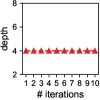
(a)

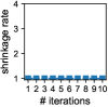
(b)

Figure 6: Trace of HP changes over iterations on spamspace: (top) tuning regularization HPs only; (bottom) tuning both regularization and architectural HPs (ours). When architecture is fixed, regularization HPs incur more magnitude changes and reach larger values to adjust model complexity. HyPer tunes complexity more flexibly by also accommodating architectural HPs.

HP Schedules over Iterations. In Fig. 6, we more closely analyze how HPs change over iterations on spamspace, comparing between (top) only tuning reg. HPs while fixing model depth and width (i.e., shrinkage rate) and (bottom) using HyPer to tune all HPs including both reg. and architectural HPs. Bottom figures show that depth remains fixed at 4, shrinkage rate increases from 1 to 2.25 (i.e., width gets reduced), dropout to 0.2, and weight decay to 0.05—overall model capacity is reduced relative to initialization. In contrast, top figures show that, when model depth and width are fixed, regularization HPs compensate more to adjust the model capacity, with a larger dropout rate at 0.4 and larger weight decay at 0.08, achieving ROC rank 0.3227 in contrast to HyPer’s 0.0555. This comparison showcases the merit of HyPer which adjusts model complexity more flexibly through accommodating a larger model space.

6 Conclusion

We introduced HyPer, a new framework for unsupervised deep outlier model selection. HyPer tackles two fundamental challenges that arise in this setting: validation in the absence of supervision and efficient search of the large model space. To this end, it employs meta-learning to train a proxy validation function on historical datasets to effectively predict model performance on a new task without labels. To speed up search, it utilizes a novel hypernetwork design that generates weights for the detection model with varying HPs including model architecture, achieving significant efficiency gains over individually training the candidate models. Extensive experiments on a large testbed with 35 benchmark datasets showed that HyPer significantly outperforms 8 simple to SOTA baselines.

Appendix

Appendix A Hypernetwork Details

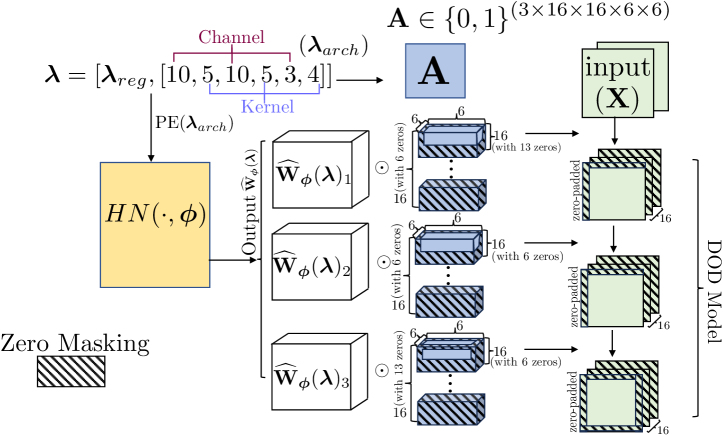
Figure A1: Illustration of the proposed HN. HN generates weights for a 3-layer convolutional networks , with channels equal to $[10,10,3]$, and kernels equal to $[5,5,4]$. The HN weights $\widehat{\mathbf{W}}_{\bm{\phi}}$ is of size $3\times 16\times 16\times 6\times 6$, and similarily we construct the same-size architecture masking $\mathbf{A}$. At the first layer, we need to pad $\mathbf{A}$ for 1 zero, among the third and fourth dimension (we pad starting from the left and from the top). This will enable us to extend $\widehat{\mathbf{W}}_{\bm{\phi}}$ to a convolutional operation of kernel size $5$, from fixed kernel size $6$. To match the padding operation, we also pad the input $\mathbf{X}$ along the first and second dimension, with 1. The rest layers follow similairly.

Architecture Masking for Convolution Operations. Since more complex data such as images and videos are used as mediums to find anomalies, many DOD models have taken convolutional networks as the backbone structure. Therefore, how to tune convolution operation within the DOD model has been an emergent problem. Here we design the input of the HN $\bm{\lambda}_{arch}$ and the architecture $\mathbf{A}$ in a format that could alter output of the HN output $\widehat{\mathbf{W}}_{\bm{\phi}}$ to adapt to various architectures.

For convolutional networks, despite that we are able to tune depths and channels, we can also include kernel sizes and dilation rate by properly padding $\widehat{\mathbf{W}}_{\bm{\phi}}$ with zeros Wang et al. [2021]. For our demonstration purposes, we only inlude the kernel size as the additional turnable variable. We make HN output $\widehat{\mathbf{W}}_{\bm{\phi}}\in\mathbbm{R}^{(D\times M_{ch}\times M_{ch}\times M_{k}\times M_{k})}$, where $D$, $M_{ch}$, $M_{k}$ represent maximum number of layers, channels, and kernel size specified in ${\bm{\Lambda}}$, respectively.

Assume $\bm{\lambda}_{arch}$ contains the abstraction of a smaller architectures, e.g. $L$ layers with corresponding channel values $\{M_{c1},M_{c2},...,M_{cL}\}$ all less than or equal to $M_{ch}$, and $\{K_{1},K_{2},...,K_{L}\}$ are less than or equal to $M_{k}$. Then, the $\bm{\lambda}_{arch}\in\mathbbm{N}^{2D}$ is given as:

$${\bm{\lambda}}_{arch}=[M_{c1},K_{1},M_{c2},K_{2},\ldots,M_{c\lfloor L/2\rfloor},K_{\lfloor L/2\rfloor},\underbracket{{0,\ldots,0}}_{\text{{\color[rgb]{0,0,0}$2(D$$-$$L)$} zeros }},M_{c\lfloor L/2\rfloor+1},K_{\lfloor L/2\rfloor+1},\ldots,M_{cL},K_{L}]\;.$$

The architecture masking $\mathbf{A}\in\{0,1\}^{(D\times M_{ch}\times M_{ch}\times M_{k}\times M_{k})}$ is constructed as the following:

$$\begin{cases}\mathbf{A}_{[l,0:\bm{\lambda}_{arch}[2\times l],:,\lfloor\frac{M_{ch}}{2}\rfloor-\lfloor\frac{\bm{\lambda}_{arch}[2\times l+1]}{2}\rfloor:\lfloor\frac{M_{ch}}{2}\rfloor+\lfloor\frac{\bm{\lambda}_{arch}[2\times l+1]}{2}\rfloor]}=1&\text{, if }l=0\\ \mathbf{A}_{[l,0:\bm{\lambda}_{arch}[2\times l],0:\bm{\lambda}_{arch}[2\times(l-z)],\lfloor\frac{M_{ch}}{2}\rfloor-\lfloor\frac{\bm{\lambda}_{arch}[2\times l+1]}{2}\rfloor:\lfloor\frac{M_{ch}}{2}\rfloor+\lfloor\frac{\bm{\lambda}_{arch}[2\times l+1]}{2}\rfloor]}=1&\text{, otherwise }\end{cases}$$ (8)

Again, $\bm{\lambda}_{arch}[2\times(l-z)]$ is the last entry corresponding to the non-zero input channel in $\bm{\lambda}_{arch}[2\times l]$. Similar to the linear operation, at layer $l$, if $\bm{\lambda}_{arch}[2\times l]$ is all zero, then the resulting $\mathbf{A}_{[l,:,:,:,:]}$ would contain only zeros and represent a "No-op" in the DOD model. Otherwise, assume we want obtain a smaller kernel size, $K_{l}\leq M_{k}$ at layer $l$, the corresponding $\mathbf{A}_{[l,:,:,:,:]}$ pads zeros around the size $M_{ch}\times k\times k$ center (See Figure A1). The masked weights $\mathbf{A}_{[l,:,:,:,:]}\odot\widehat{\mathbf{W}}_{\bm{\phi},l}$ are equivalent to obtaining smaller-size kernel weights. Notice that, when kernel sizes are different, the output of the layer’s operation will also differ (smaller kernels would result in larger output size); therefore, we need to guarantee the spatial size by similarity padding zeros around the input of that convolutional layer. The padding is similar to how we construct the architecture masking $\mathbf{A}$ and similar to the padding approach discussed in Wang et al. [2021].

Extending to Other Architectures. We envision our proposed HN can be extended to other architectures, for example, to tune the number of attention heads and dimensions of query, key and values in the multi-headed attention mechanism Vaswani et al. [2017]. We will continuously work on the implementations for other architectures, as more complex DOD models are developed recently.

Appendix B Meta-Training Details

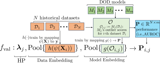
Figure B2: Illustration of the $f_{\text{val}}$. We use all historical datasets (i.e., $\mathbf{X}$ and ground-truth labels $\mathbf{y}$) to train the data embeddings and historical embeddings, during which we obtain performance $\mathbf{P}$ on the DOD models’ outlier scores $\mathcal{O}$. During the offline phase, We train $h(\cdot)$, $g(\cdot)$, and $f_{\text{val}}$. During the online model selection time, $f_{\text{val}}$ gives the performance estimation of a DOD model (with a specific HP ${\bm{\lambda}}$), on the embedding of the test dataset.

We provide details of training $f_{\text{val}}$ in this section. Fig. B2 illustrate the training of $f_{\text{val}}$ in Eq. (4).

Data Embeddings. . We employ feature hashing Weinberger et al. [2009] to address the issue of that datasets may have different feature and sample sizes. Specifically, a hashing function $\psi(\cdot)$, is employed to project each dataset to a $k$-dimensional unified feature space, regardless of the number of features in the original data. To ensure sufficient expressiveness, the projection dimension should not be too small (e.g., $k=256$ in our experiments).

Subsequently, we train a cross-dataset feature extractor $h(\cdot)$, a fully connected neural network, to map hashed samples to their corresponding outlier labels, i.e. $h:\psi(\mathbf{X}_{i})\mapsto\mathbf{y}_{i}$ for the $i$-th dataset. Finally, we use max-pooling to aggregate sample-wise representations into dataset-wise embeddings, denoted by $\text{pool}\{h(\psi({\color[rgb]{0,0,0}\mathbf{X}_{i}}))\}$. The overall goal of $h(\cdot)$ is to capture outlying characteristics of datasets, as demonstrated in the left middle of Fig. B2.

Model Embeddings . In addition to data embeddings, we have also designed model embeddings to capture the impact of model changes on the detection performance. To achieve this, existing work uses internal performance measures (IPMs) as model embeddings Zhao et al. [2022]. IPMs are a set of unsupervised performance evaluation metrics for OD that solely rely on model outputs and/or input features. They serve as weak proxies for model performance (more details can be found in Ma et al. [2023]). However, the design of IPMs is typically handcrafted, and their computation at runtime can be computationally expensive.

To represent a trained DOD model more systematically, we utilize a neural network denoted as $g(\cdot)$, which maps the output outlier scores of the model to the corresponding detection performance, i.e. $g:\mathcal{O}_{i,j}\mapsto\mathbf{P}_{i,j}$. To handle the variability in the size of outlier scores, which can arise from differences in sample sizes across datasets, we employ the DeepSet architecture Zaheer et al. [2017] for $g(\cdot)$. The DeepSet architecture is designed to leverage the inherent permutation invariance of sets, meaning that the order of elements in a set does not affect its overall meaning. Similarly, the order of outlier scores does not impact the overall detection performance. In our approach, we use the output of the pooling layer in the DeepSet architecture, denoted as $\text{pool}({g({\color[rgb]{0,0,0}\mathcal{O}_{i,j}})})$, as the model embedding. This pooling layer output effectively captures the information from the outlier scores and produces a fixed-size representation of the model’s performance, as shown in the right middle of Fig. B2.

Obtaining outlier scores $\mathcal{O}_{i,j}$ requires training the DOD model, which can be computationally expensive. To speed up this process for meta-training, we use HN-generated weights other than training individual DOD models from scratch, to obtain $\widehat{\mathcal{O}}_{i,j}:=M_{j}(\mathcal{D}_{i};\widehat{\mathbf{W}}^{(i)}_{\bm{\phi}}({\bm{\lambda}_{j}}))$, where $\widehat{\mathbf{W}}^{(i)}_{\bm{\phi}}({\bm{\lambda}_{j}})$ denotes model $M_{j}$’s weights as generated by our HN trained on $\mathcal{D}_{i}$, and ${\bm{\lambda}}_{j}$ are over existing ${\bm{\lambda}}_{\mathbf{meta}}$.

Training $f_{\text{val}}$. The goal of $f_{\text{val}}$ is to map the aforementioned components, e.g., HPs, data embeddings, and model embeddings, onto the corresponding model performance across $N$ historical datasets and $m$ models with varying HP configurations. The choice of $f_{\text{val}}$ can be flexible: we use lightGBM Ke et al. [2017] in this work; although one may use any regressor.

We decide the hyperparameters associated with $\psi(\cdot)$, $h(\cdot)$, $g(\cdot)$, and $f_{\text{val}}$ by the cross-validation of the historical datasets. The goal is to optimize the performance of $f_{\text{val}}$ on the historical datasets. We provide additional meta-training details in §C.2.

Appendix C Additional Experiment Settings and Results

C.1 Datasets

To build a comprehensive testbed, we use 15 OD datasets from the DAMI repository and 20 OD datasets from the ODDS repository. All of these benchmark datasets are widely used in OD research. We provide the dataset summary in Table C1.

Table C1: The tabular testbed includes 35 datasets from DAMI and ODDS repositories.

Dataset	Source	#Samples	#Dims	%Outlier
DAMI_Annthyroid	DAMI	7129	21	7.49
DAMI_Cardiotocography	DAMI	2114	21	22.04
DAMI_Glass	DAMI	214	7	4.21
DAMI_HeartDisease	DAMI	270	13	44.44
DAMI_PageBlocks	DAMI	5393	10	9.46
DAMI_PenDigits	DAMI	9868	16	0.2
DAMI_Pima	DAMI	768	7	34.9
DAMI_Shuttle	DAMI	1013	9	1.28
DAMI_SpamBase	DAMI	4207	57	39.91
DAMI_Stamps	DAMI	340	9	9.12
DAMI_Waveform	DAMI	3443	21	2.9
DAMI_WBC	DAMI	223	9	4.48
DAMI_WDBC	DAMI	367	30	2.72
DAMI_Wilt	DAMI	4819	5	5.33
DAMI_WPBC	DAMI	198	33	23.74
ODDS_annthyroid	ODDS	7200	6	7.42
ODDS_arrhythmia	ODDS	452	274	14.6
ODDS_breastw	ODDS	683	9	34.99
ODDS_glass	ODDS	214	9	4.21
ODDS_ionosphere	ODDS	351	33	35.9
ODDS_letter	ODDS	1600	32	6.25
ODDS_lympho	ODDS	148	18	4.05
ODDS_mammography	ODDS	11183	6	2.32
ODDS_mnist	ODDS	7603	100	9.21
ODDS_musk	ODDS	3062	166	3.17
ODDS_optdigits	ODDS	5216	64	2.88
ODDS_pendigits	ODDS	6870	16	2.27
ODDS_satellite	ODDS	6435	36	31.64
ODDS_satimage-2	ODDS	5803	36	1.22
ODDS_speech	ODDS	3686	400	1.65
ODDS_thyroid	ODDS	3772	6	2.47
ODDS_vertebral	ODDS	240	6	12.5
ODDS_vowels	ODDS	1456	12	3.43
ODDS_wbc	ODDS	378	30	5.56
ODDS_wine	ODDS	129	13	7.75

C.2 Algorithm Settings and Baselines

Table C2: HyPer and baselines for time and performance comparison with categorization by whether it selects models (2nd column), uses meta-learning (3rd column), and requires model building at the test time (4th column). Overall, HyPer (with patience $p=3$) achieves the best detection performances (also see Fig. 4 and 5). Compared to the SOTA ELECT, HyPer has markedly shorter offline and online time with the help of HN.

Method	Model Selection	Meta Learning	Zero shot	Offline Time (mins.)	Average Online Time (mins.)	Median Online Time (mins.)	Avg. ROC Rank ($\downarrow$ better)
Default	✗	✗	✓	N/A	0	0	0.5954
Random	✗	✗	✓	N/A	0	0	0.5603
MC	✓	✗	✗	N/A	215	277	0.5642
GB	✓	✓	✓	7,461	0	0	0.4668
ISAC	✓	✓	✓	7,466	1	1	0.4181
AS	✓	✓	✓	7,465	1	1	0.5222
MetaOD	✓	✓	✓	7,525	1	1	0.3918
ELECT	✓	✓	✗	7,611	59	71	0.3621
Ours	✓	✓	✗	1,320	14	17	0.2954

In this section, we present additional experiment settings and describe the baselines. For detailed implementation information, please see https://github.com/inreview23/HYPER.

Setting of the HN: The HN utilized in the experiments consists of two hidden layers, each containing 200 neurons. It is configured with a learning rate of 1e-4, a dropout rate of 0.2, and a batch size of 512. We find this setting give enough capacity to generate various weights for linearAEs. Because of the meta-learning setting, the hyperparameters of HN can be tested with validation data and test results, on historical data.

Meta-training for $f_{\text{val}}$. Table C6 includes the HP search space for training. In the table, compression rate refers to how many of the widths to shrink between two adjacent layers. For example, if the first layer has width of $6$, compression_rate equals $2$ would gvie the next layer width equal to $3$. We also notice that some datasets may have smaller numbers of features. Thus, with the corresponding compression rate, we also have discretized the width to the nearest integer number. Thus, for some datasets, the HP search space will be smaller than $240$.

HN (Re-)Training during the Online Phase: In order to facilitate effective local re-training, we set a training epoch of $T=100$ for each iteration, indicating the sampling of 100 local HPs for HN retraining. In Eq. (6), we designate the number of sampled HPs and the sampling factor as 500, i.e., $V_{\lambda}=V_{\sigma}=500$. The minimum depth and maximum depth of the searched DOD models are set to 2 and 8, respectively. Essentially, we tune the DOD model depth within the integer range of 2 to 8.

Convergence: To achieve favorable performance within a reasonable timeframe, we set the patience value as $p=3$ in the experiment. Further analysis for the impact of patience is available in §C.3.2.

Baselines: We have incorporated 8 baselines, encompassing a spectrum from simple to state-of-the-art (SOTA) approaches. Table C2 offers a comprehensive conceptual comparison of these baselines.

(i) no model selection:

1. Default employs the default HPs utilized in the widely-used OD library PyOD Zhao et al. [2019]. This serves as the default option for practitioners when no additional information is available.

2. Random randomly selects an HP/model (the reported performance represents the expected value obtained by averaging across all DOD models).

(ii) model selection without meta-learning:

1. MC Ma et al. [2023] utilizes the consensus among a group of DOD models to assess the performance of a model. A model is considered superior if its outputs are closer to the consensus of the group. MC necessitates the construction of a model group during the testing phase. For more details, please refer to a recent survey Ma et al. [2021].

(iii) model selection by meta-learning requires first building a corpus of historical datasets on a group of defined DOD models and then selecting the best from the model set at the test time. Although these baselines utilize meta-learning, none of them take advantage of the HN for acceleration.

1. Global Best (GB) selects the best-performing model based on the average performance across historical datasets.

2. ISAC Kadioglu et al. [2010] groups historical datasets into clusters and predicts the cluster of the test data, subsequently outputting the best model from the corresponding cluster.

3. ARGOSMART (AS) Nikolic et al. [2013] measures the similarity between the test dataset and all historical datasets, and then outputs the best model from the most similar historical dataset.

4. MetaOD Zhao et al. [2021] employs matrix factorization to capture both dataset similarity and model similarity, representing one of the state-of-the-art methods for unsupervised OD model selection.

5. ELECT Zhao et al. [2022] iteratively identifies the best model for the test dataset based on performance similarity to the historical dataset. Unlike the above meta-learning approaches, ELECT requires model building during the testing phase to compute performance-based similarity.

Baseline Model Set. We use the same HP search spaces for baseline models as well as the HN-trained models. Table C6 provides the detailed HP search space.

C.3 Additional Ablations

C.3.1 Effect of Meta-initialization

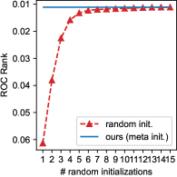
(a)

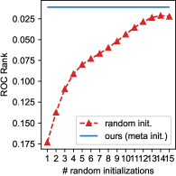
(b)

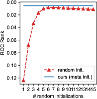
(c)

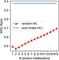
(d)

Figure C3: Comparison of ROC Rank (lower is better) of HyPer with meta-initialization (in blue) with increasing numbers of randomly initialized HNs. For instance, it needs 9 randomly initialized HNs to achieve the same performance as HyPer on ODDS_wine. In general, HyPer shows better efficiency in finding a good model with much less running time.

As mentioned in §4.2, HyPer initializes the HPs to the “global best HPs" derived from the historical training datasets. Specifically, in each fold comprising 7 test datasets, we utilize the HPs that yield the best average performance across the remaining 28 training datasets as the initial HPs. This meta-initialization approach leverages meta-learning to initialize HyPer with a potentially promising HP configuration.

In Figure C3, we demonstrate the effectiveness of meta-initialization by comparing it with random initialization on five datasets. In addition to utilizing meta-initialization, one could run HyPer multiple times with randomly initialized HPs and select the best model based on $f_{\text{val}}$. However, it should be noted that $f_{\text{val}}$ serves as a proxy validator rather than ground truth. Therefore, including more randomly initialized HNs does not guarantee a monotonic improvement in the selected model’s performance. Nonetheless, increasing the number of random initializations is likely to yield a better performance by exploring a broader range of search spaces.

To simulate this scenario, we vary the number of random initializations (x-axis) and record all the $f_{\text{val}}$ values along with the corresponding ROC Rank. For each dataset, we select the best model based on $f_{\text{val}}$ across all trials. We increase the number of random trials from 1 to 15, where the highest $f_{\text{val}}$ value among the 15 random initialized trials is chosen as the best model. The y-axis represents the average performance from independent trials.

The figure clearly demonstrates the advantage of meta-initialization as a strong starting point for HyPer’s HP tuning. For example, on the ODDS_wine dataset (refer to Fig. 3(a)), it requires 9 randomly initialized HNs to attain the same performance as our approach with meta-initialization, showing a 9-fold increase in the time required for online selection. In other cases (Fig. 3(b), 3(c), and 3(d)), training 15 randomly initialized HNs fails to achieve the same performance as meta-initialization, further validating its advantages.

C.3.2 Effect of Patience

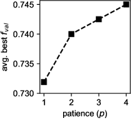
(a)

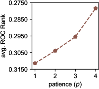
Figure C4: Analysis of the effect of patience $p$: (left) avg. $f_{\text{val}}$ value change when increasing $p$ from 1 to 4; (right) avg. ROC Rank with increasing $p$. Larger $p$ leads to more exploration and likely better performance.

As described in §4.1, the convergence criterion for HyPer is based on the highest predicted performance by $f_{\text{val}}$ remaining unchanged for $p$ consecutive iterations. A larger value of $p$, also known as “patience," requires more iterations for convergence but is likely to yield better results. As illustrated in Fig. C4, increasing the value of $p$ allows for more exploration and potentially better performance. However, this also prolongs the convergence time.

In our experiments, we set $p=3$ to balance performance and runtime. The specific value of $p$ can be determined through cross-validation over the historical datasets, taking into account the specific criteria and requirements of the underlying application.

C.4 Additional Results

In addition to the distribution plot in Fig. 5, we provide the $p$-values of Wilcoxon signed rank test between HyPer and baselines in C3. See §5 for the experiment analysis.

Table C3: Pairwise statistical tests between HyPer and baselines by Wilcoxon signed rank test. HyPer are statistically better than the baselines and its variants at different significance levels. See Fig.5 for distribution rank with statistical comparison.

Ours	Baseline	p-value
Ours	Default	0.0016
Ours	Random	0.0001
Ours	ISAC	0.0025
Ours	AS	0.0052
Ours	MetaOD	0.0030
Ours	Global Best	0.0015
Ours	MC	0.0005
Ours	ELECT	0.0568
Ours	Ours (reg&width)	0.0001
Ours	Ours (reg&depth)	0.0001
Ours	Ours (reg only)	0.0001

Table C4: ROC of the evaluated methods. The best method per dataset (row) is highlighted in bold.

Dataset	Default	Random	MC	GB	ISAC	AS	MetaOD	ELECT	Ours
DAMI_Annthyroid	0.7124	0.5972	0.6123	0.5929	0.6018	0.5873	0.6050	0.6148	0.5888
DAMI_Cardiotocography	0.7159	0.7202	0.7024	0.7740	0.7571	0.6940	0.6458	0.7818	0.7866
DAMI_Glass	0.7442	0.7055	0.6304	0.7244	0.6699	0.7230	0.7225	0.7431	0.6917
DAMI_HeartDisease	0.3045	0.4276	0.4214	0.5250	0.5382	0.4214	0.5312	0.5348	0.5926
DAMI_PageBlocks	0.8722	0.9107	0.9219	0.9162	0.9255	0.9002	0.6247	0.8791	0.9215
DAMI_PenDigits	0.3837	0.5248	0.5422	0.5491	0.5069	0.6953	0.6278	0.5084	0.6792
DAMI_Pima	0.4005	0.5508	0.4855	0.6216	0.6279	0.6158	0.4862	0.6281	0.6595
DAMI_Shuttle	0.6453	0.9462	0.9400	0.9342	0.9436	0.9530	0.5525	0.9405	0.9391
DAMI_SpamBase	0.5208	0.5232	0.4907	0.5210	0.5263	0.5552	0.5307	0.5135	0.5525
DAMI_Stamps	0.8687	0.8687	0.8926	0.8981	0.9079	0.8618	0.7112	0.8897	0.9003
DAMI_Waveform	0.6810	0.6772	0.6560	0.6941	0.6924	0.6890	0.6900	0.7019	0.6929
DAMI_WBC	0.7493	0.9769	0.9770	0.9682	0.9742	0.9779	0.9809	0.9779	0.9826
DAMI_WDBC	0.8092	0.8366	0.8146	0.8597	0.8683	0.8092	0.8361	0.8213	0.9039
DAMI_Wilt	0.5080	0.4524	0.4832	0.4653	0.4700	0.4700	0.4714	0.4700	0.3709
DAMI_WPBC	0.4090	0.4464	0.3972	0.4679	0.4548	0.4285	0.4456	0.4726	0.4824
ODDS_annthyroid	0.7353	0.6981	0.6963	0.6982	0.7067	0.7067	0.6903	0.7058	0.7014
ODDS_arrhythmia	0.7769	0.7786	0.7810	0.7767	0.7831	0.7798	0.7824	0.7807	0.7827
ODDS_breastw	0.5437	0.6187	0.8939	0.9071	0.8032	0.7986	0.5913	0.8649	0.9045
ODDS_glass	0.6195	0.5849	0.5453	0.5897	0.5962	0.5962	0.5654	0.5957	0.5993
ODDS_ionosphere	0.8708	0.8497	0.8711	0.8252	0.8422	0.8350	0.8727	0.8686	0.8509
ODDS_letter	0.5555	0.5758	0.5918	0.6068	0.6244	0.6155	0.6446	0.6211	0.6102
ODDS_lympho	0.9096	0.9959	0.9988	0.9842	0.9929	0.9953	0.9971	1.0000	0.9925
ODDS_mammography	0.5287	0.7612	0.7233	0.8362	0.7189	0.7116	0.8640	0.7673	0.8542
ODDS_mnist	0.8518	0.8915	0.8662	0.8959	0.9011	0.8580	0.9070	0.9032	0.8994
ODDS_musk	0.9940	1.0000	1.0000	1.0000	1.0000	1.0000	1.0000	1.0000	1.0000
ODDS_optdigits	0.5104	0.4950	0.5092	0.4806	0.5115	0.5171	0.4973	0.5338	0.5584
ODDS_pendigits	0.9263	0.9295	0.9265	0.9305	0.9208	0.9386	0.9360	0.9346	0.9435
ODDS_satellite	0.7681	0.7284	0.7445	0.7352	0.7433	0.7324	0.7486	0.7571	0.7432
ODDS_satimage-2	0.9707	0.9826	0.9865	0.9744	0.9838	0.9798	0.9871	0.9786	0.9853
ODDS_speech	0.4761	0.4756	0.4692	0.4726	0.4832	0.4692	0.4706	0.4774	0.4707
ODDS_thyroid	0.9835	0.9661	0.9652	0.9535	0.9635	0.9652	0.9740	0.9689	0.9667
ODDS_vertebral	0.6019	0.5378	0.5629	0.5253	0.4602	0.5629	0.4657	0.5629	0.4757
ODDS_vowels	0.4897	0.5903	0.5965	0.6309	0.6414	0.6686	0.6216	0.5247	0.6686
ODDS_wbc	0.4146	0.8401	0.7640	0.8808	0.8745	0.8469	0.8770	0.8469	0.9289
ODDS_wine	0.7864	0.5430	0.4084	0.7539	0.5387	0.4084	0.6296	0.6218	0.8287

We present the full results in Table C4 and C5. Note that ROC Rank is based on each method’s performance in regard to the baseline model set’s performance described in §C.2.

Table C5: ROC Rank (smaller the better) of the evaluated methods. The best method per dataset (row) is highlighted in bold.

Dataset	Default	Random	MC	GB	ISAC	AS	MetaOD	ELECT	Ours
DAMI_Annthyroid	0.0079	0.5317	0.1111	0.6031	0.4206	0.7143	0.3492	0.0794	0.6984
DAMI_Cardiotocography	0.5635	0.4683	0.6190	0.0476	0.1984	0.6825	1.0000	0.0476	0.0238
DAMI_Glass	0.0556	0.7222	0.9365	0.1984	0.9048	0.5556	0.5635	0.0595	0.8016
DAMI_HeartDisease	0.9841	0.5556	0.5873	0.1032	0.0238	0.5714	0.0476	0.0317	0.0079
DAMI_PageBlocks	1.0000	0.4921	0.2698	0.4048	0.1667	0.7937	1.0000	0.9841	0.2937
DAMI_PenDigits	0.9048	0.5317	0.4722	0.4206	0.6429	0.0714	0.1349	0.6270	0.0794
DAMI_Pima	1.0000	0.5159	0.9603	0.1508	0.0635	0.2540	0.6508	0.0556	0.0079
DAMI_Shuttle	1.0000	0.4444	0.9365	1.0000	0.5635	0.2381	1.0000	0.7302	0.9683
DAMI_SpamBase	0.6349	0.5556	0.9921	0.6270	0.3571	0.0397	0.1825	0.8016	0.0556
DAMI_Stamps	0.5238	0.5238	0.2619	0.1587	0.0635	0.6032	1.0000	0.2857	0.1349
DAMI_Waveform	0.4762	0.5556	0.8175	0.1429	0.2143	0.2619	0.2619	0.0556	0.1905
DAMI_WBC	1.0000	0.7381	0.7381	0.9921	0.9365	0.5873	0.0079	0.5873	0.0079
DAMI_WDBC	0.8095	0.5397	0.7619	0.2381	0.0873	0.8016	0.5556	0.6984	0.0159
DAMI_Wilt	0.0159	0.7302	0.0238	0.7143	0.7143	0.7143	0.0397	0.7143	0.9762
DAMI_WPBC	1.0000	0.4365	1.0000	0.2302	0.3413	0.8175	0.4524	0.1667	0.0079
ODDS_annthyroid	0.0397	0.3651	0.3889	0.3571	0.2381	0.2302	0.7937	0.2540	0.3016
ODDS_arrhythmia	0.7063	0.5556	0.2302	0.7222	0.1270	0.3889	0.1587	0.2857	0.1349
ODDS_breastw	0.5794	0.5317	0.1032	0.0714	0.3095	0.3333	0.5317	0.1905	0.0794
ODDS_glass	0.2143	0.3571	0.9048	0.3333	0.2937	0.2857	0.5159	0.3095	0.2857
ODDS_ionosphere	0.0872	0.4841	0.0873	0.9683	0.5714	0.8254	0.0476	0.1587	0.4603
ODDS_letter	0.6746	0.6429	0.4762	0.3333	0.0476	0.1349	0.0079	0.0635	0.2539
ODDS_lympho	1.0000	0.4921	0.2143	1.0000	0.9365	0.6429	0.4365	0.0437	0.9365
ODDS_mammography	1.0000	0.3889	0.8968	0.2381	0.9127	0.9286	0.0317	0.3571	0.0714
ODDS_mnist	0.9286	0.6746	0.8651	0.6190	0.4603	0.9048	0.1270	0.3492	0.5238
ODDS_musk	1.0000	0.8810	0.3730	0.3730	0.3730	0.3730	0.3730	0.3730	0.3730
ODDS_optdigits	0.3651	0.5714	0.4048	0.6825	0.3333	0.2063	0.5238	0.1032	0.0397
ODDS_pendigits	0.7222	0.6587	0.7222	0.6269	0.8254	0.1825	0.2619	0.3730	0.0397
ODDS_satellite	0.0238	0.7222	0.2778	0.6825	0.3651	0.7063	0.0873	0.0317	0.3889
ODDS_satimage-2	1.0000	0.6270	0.0556	0.9841	0.4048	0.8413	0.0317	0.9048	0.0714
ODDS_speech	0.4048	0.4286	0.8651	0.5873	0.1825	0.8730	0.6825	0.3810	0.6746
ODDS_thyroid	0.0079	0.4841	0.5556	1.0000	0.6905	0.5635	0.0476	0.4603	0.4762
ODDS_vertebral	0.0159	0.6984	0.3571	0.7381	0.9127	0.5159	0.8730	0.3571	0.8254
ODDS_vowels	1.0000	0.5873	0.5397	0.3254	0.2063	0.1111	0.3730	0.8016	0.1111
ODDS_wbc	1.0000	0.6349	0.9762	0.1746	0.2460	0.5714	0.2063	0.5714	0.0079
ODDS_wine	0.0238	0.4841	0.9603	0.0397	0.5000	0.9603	0.3333	0.3810	0.0159
Avg. ROC Rank	0.5954	0.5603	0.5642	0.4668	0.4181	0.5222	0.3918	0.3621	0.2954

Table C6: Hyperparameter search space for both free-range and HN models. We give the list of HPs as well as the range of the selected HPs.

List of Hyperparameters (HPs)	# HPs
n_layers: [2,4,6,8]	4
compression_rate: [1.0,1.2,1.4,1.6,1.8,2.0,2.2,2.4,2.6,2.8,3.0]	10
dropout: [0.0,0.2,0.4]	3
weight_decay: [0.0,1e-6,1e-5]	3
Total Number:	240

References

- Pang et al. [2021] Guansong Pang, Chunhua Shen, Longbing Cao, and Anton Van Den Hengel. Deep learning for anomaly detection: A review. ACM computing surveys (CSUR), 54(2):1–38, 2021.
- Ruff et al. [2021] Lukas Ruff, Jacob R Kauffmann, Robert A Vandermeulen, Grégoire Montavon, Wojciech Samek, Marius Kloft, Thomas G Dietterich, and Klaus-Robert Müller. A unifying review of deep and shallow anomaly detection. Proceedings of the IEEE, 109(5):756–795, 2021.
- Ding et al. [2022] Xueying Ding, Lingxiao Zhao, and Leman Akoglu. Hyperparameter sensitivity in deep outlier detection: Analysis and a scalable hyper-ensemble solution. In Alice H. Oh, Alekh Agarwal, Danielle Belgrave, and Kyunghyun Cho, editors, Advances in Neural Information Processing Systems, 2022.
- Bergstra and Bengio [2012] James Bergstra and Yoshua Bengio. Random search for hyper-parameter optimization. J. Mach. Learn. Res., 13:281–305, 2012. URL http://dblp.uni-trier.de/db/journals/jmlr/jmlr13.html#BergstraB12.
- Li et al. [2017] Lisha Li, Kevin G. Jamieson, Giulia DeSalvo, Afshin Rostamizadeh, and Ameet Talwalkar. Hyperband: A novel bandit-based approach to hyperparameter optimization. J. Mach. Learn. Res., 18:185:1–185:52, 2017. URL http://dblp.uni-trier.de/db/journals/jmlr/jmlr18.html#LiJDRT17.
- Shahriari et al. [2016] Bobak Shahriari, Kevin Swersky, Ziyu Wang, Ryan P. Adams, and Nando de Freitas. Taking the human out of the loop: A review of bayesian optimization. Proc. IEEE, 104(1):148–175, 2016. doi: 10.1109/JPROC.2015.2494218. URL https://doi.org/10.1109/JPROC.2015.2494218.
- Li et al. [2021] Yuening Li, Zhengzhang Chen, Daochen Zha, Kaixiong Zhou, Haifeng Jin, Haifeng Chen, and Xia Hu. Autood: Neural architecture search for outlier detection. In 37th IEEE International Conference on Data Engineering, ICDE 2021, Chania, Greece, April 19-22, 2021, pages 2117–2122. IEEE, 2021. doi: 10.1109/ICDE51399.2021.00210. URL https://doi.org/10.1109/ICDE51399.2021.00210.
- Li et al. [2020] Yuening Li, Daochen Zha, Praveen Kumar Venugopal, Na Zou, and Xia Hu. Pyodds: An end-to-end outlier detection system with automated machine learning. In Amal El Fallah Seghrouchni, Gita Sukthankar, Tie-Yan Liu, and Maarten van Steen, editors, Companion of The 2020 Web Conference 2020, Taipei, Taiwan, April 20-24, 2020, pages 153–157. ACM / IW3C2, 2020. doi: 10.1145/3366424.3383530. URL https://doi.org/10.1145/3366424.3383530.
- Lai et al. [2021] Kwei-Herng Lai, Daochen Zha, Guanchu Wang, Junjie Xu, Yue Zhao, Devesh Kumar, Yile Chen, Purav Zumkhawaka, Minyang Wan, Diego Martinez, and Xia Hu. TODS: an automated time series outlier detection system. In Thirty-Fifth AAAI Conference on Artificial Intelligence, AAAI 2021, Thirty-Third Conference on Innovative Applications of Artificial Intelligence, IAAI 2021, The Eleventh Symposium on Educational Advances in Artificial Intelligence, EAAI 2021, Virtual Event, February 2-9, 2021, pages 16060–16062. AAAI Press, 2021. URL https://ojs.aaai.org/index.php/AAAI/article/view/18012.
- Goix [2016] Nicolas Goix. How to evaluate the quality of unsupervised anomaly detection algorithms? CoRR, abs/1607.01152, 2016. URL http://dblp.uni-trier.de/db/journals/corr/corr1607.html#Goix16.
- Marques et al. [2015] Henrique O. Marques, Ricardo J. G. B. Campello, Arthur Zimek, and Jörg Sander. On the internal evaluation of unsupervised outlier detection. In SSDBM, pages 7:1–7:12. ACM, 2015. URL http://dblp.uni-trier.de/db/conf/ssdbm/ssdbm2015.html#MarquesCZS15.
- Duan et al. [2020] Sunny Duan, Loic Matthey, Andre Saraiva, Nick Watters, Christopher Burgess, Alexander Lerchner, and Irina Higgins. Unsupervised model selection for variational disentangled representation learning. In ICLR. OpenReview.net, 2020. URL http://dblp.uni-trier.de/db/conf/iclr/iclr2020.html#DuanMSWBLH20.
- Lin et al. [2020] Zinan Lin, Kiran Thekumparampil, Giulia Fanti, and Sewoong Oh. InfoGAN-CR and ModelCentrality: Self-supervised model training and selection for disentangling GANs. In International Conference on Machine Learning, pages 6127–6139. PMLR, 2020.
- Martin et al. [2021] Charles H Martin, Tongsu Peng, and Michael W Mahoney. Predicting trends in the quality of state-of-the-art neural networks without access to training or testing data. Nature Communications, 12(1):4122, 2021.
- Ma et al. [2023] Martin Q Ma, Yue Zhao, Xiaorong Zhang, and Leman Akoglu. The need for unsupervised outlier model selection: A review and evaluation of internal evaluation strategies. ACM SIGKDD Explorations Newsletter, 25(1), 2023.
- Zhao et al. [2021] Yue Zhao, Ryan Rossi, and Leman Akoglu. Automatic unsupervised outlier model selection. In Thirty-Fifth Conference on Neural Information Processing Systems, 2021.
- Zhao et al. [2022] Yue Zhao, Sean Zhang, and Leman Akoglu. Toward unsupervised outlier model selection. In IEEE International Conference on Data Mining, ICDM, pages 773–782. IEEE, 2022.
- Feurer and Hutter [2019] Matthias Feurer and Frank Hutter. Hyperparameter optimization. Automated machine learning: Methods, systems, challenges, pages 3–33, 2019.
- MacKay et al. [2019] Matthew MacKay, Paul Vicol, Jonathan Lorraine, David Duvenaud, and Roger B. Grosse. Self-tuning networks: Bilevel optimization of hyperparameters using structured best-response functions. In ICLR (Poster). OpenReview.net, 2019.
- Zhao et al. [2019] Yue Zhao, Zain Nasrullah, and Zheng Li. Pyod: A python toolbox for scalable outlier detection. Journal of Machine Learning Research, 20:1–7, 2019.
- Campos et al. [2016a] Guilherme Oliveira Campos, Arthur Zimek, Jörg Sander, Ricardo J. G. B. Campello, Barbora Micenková, Erich Schubert, Ira Assent, and Michael E. Houle. On the evaluation of unsupervised outlier detection: measures, datasets, and an empirical study. Data Min. Knowl. Discov., 30(4):891–927, 2016a.
- Ha et al. [2017] David Ha, Andrew M. Dai, and Quoc V. Le. Hypernetworks. In ICLR (Poster). OpenReview.net, 2017.
- Brock et al. [2018] Andrew Brock, Theodore Lim, James M. Ritchie, and Nick Weston. Smash: One-shot model architecture search through hypernetworks. In ICLR (Poster). OpenReview.net, 2018.
- Zhang et al. [2019] Chris Zhang, Mengye Ren, and Raquel Urtasun. Graph hypernetworks for neural architecture search. In ICLR (Poster). OpenReview.net, 2019.
- Knyazev et al. [2021] Boris Knyazev, Michal Drozdzal, Graham W Taylor, and Adriana Romero Soriano. Parameter prediction for unseen deep architectures. Advances in Neural Information Processing Systems, 34:29433–29448, 2021.
- Przewięźlikowski et al. [2022] Marcin Przewięźlikowski, Przemysław Przybysz, Jacek Tabor, M Zięba, and Przemysław Spurek. Hypermaml: Few-shot adaptation of deep models with hypernetworks. arXiv preprint arXiv:2205.15745, 2022.
- von Oswald et al. [2020] Johannes von Oswald, Christian Henning, Benjamin F. Grewe, and João Sacramento. Continual learning with hypernetworks. In International Conference on Learning Representations, 2020. URL https://arxiv.org/abs/1906.00695.
- Schmidhuber [1992] Jürgen Schmidhuber. Learning to control fast-weight memories: An alternative to dynamic recurrent networks. Neural Computation, 4(1):131–139, 1992.
- Wang et al. [2021] Xiaoxing Wang, Chao Xue, Junchi Yan, Xiaokang Yang, Yonggang Hu, and Kewei Sun. Mergenas: Merge operations into one for differentiable architecture search. In Proceedings of the Twenty-Ninth International Conference on International Joint Conferences on Artificial Intelligence, pages 3065–3072, 2021.
- Vaswani et al. [2017] Ashish Vaswani, Noam Shazeer, Niki Parmar, Jakob Uszkoreit, Llion Jones, Aidan N Gomez, Ł ukasz Kaiser, and Illia Polosukhin. Attention is all you need. In I. Guyon, U. Von Luxburg, S. Bengio, H. Wallach, R. Fergus, S. Vishwanathan, and R. Garnett, editors, Advances in Neural Information Processing Systems, volume 30. Curran Associates, Inc., 2017. URL https://proceedings.neurips.cc/paper_files/paper/2017/file/3f5ee243547dee91fbd053c1c4a845aa-Paper.pdf.
- Weinberger et al. [2009] Kilian Weinberger, Anirban Dasgupta, John Langford, Alex Smola, and Josh Attenberg. Feature hashing for large scale multitask learning. In Proceedings of the 26th annual international conference on machine learning, pages 1113–1120, 2009.
- Zaheer et al. [2017] Manzil Zaheer, Satwik Kottur, Siamak Ravanbakhsh, Barnabas Poczos, Russ R Salakhutdinov, and Alexander J Smola. Deep sets. Advances in neural information processing systems, 30, 2017.
- Ke et al. [2017] Guolin Ke, Qi Meng, Thomas Finley, Taifeng Wang, Wei Chen, Weidong Ma, Qiwei Ye, and Tie-Yan Liu. Lightgbm: A highly efficient gradient boosting decision tree. Advances in neural information processing systems, 30, 2017.
- Rayana [2016] Shebuti Rayana. ODDS library, 2016.
- Campos et al. [2016b] Guilherme Oliveira Campos, Arthur Zimek, Jörg Sander, Ricardo J. G. B. Campello, Barbora Micenková, Erich Schubert, Ira Assent, and Michael E. Houle. On the evaluation of unsupervised outlier detection. DAMI, 30(4):891–927, 2016b.
- Kadioglu et al. [2010] Serdar Kadioglu, Yuri Malitsky, Meinolf Sellmann, and Kevin Tierney. Isac - instance-specific algorithm configuration. In ECAI, volume 215, pages 751–756, 2010.
- Nikolic et al. [2013] Mladen Nikolic, Filip Maric, and Predrag Janicic. Simple algorithm portfolio for sat. Artif. Intell. Rev., 40(4):457–465, 2013.
- Groggel [2000] David J. Groggel. Practical nonparametric statistics. Technometrics, 42(3):317–318, 2000.
- Ma et al. [2021] Xiaoxiao Ma, Jia Wu, Shan Xue, Jian Yang, Chuan Zhou, Quan Z Sheng, Hui Xiong, and Leman Akoglu. A comprehensive survey on graph anomaly detection with deep learning. IEEE Transactions on Knowledge and Data Engineering, 2021.