Spin vectors in the Koronis family: V. Resolving the ambiguous rotation period of (3032) Evans

Abstract

A sidereal rotation counting approach is demonstrated by resolving an ambiguity in the synodic rotation period of Koronis family member (3032) Evans, whose rotation lightcurves’ features did not easily distinguish between doubly- and quadruply-periodic. It confirms that Evans’s spin rate does not exceed the rubble-pile spin barrier and thus presents no inconsistency with being a $\sim$14-km reaccumulated object. The full spin vector solution for Evans is comparable to those for the known prograde low-obliquity comparably-fast rotators in the Koronis family, consistent with having been spun up by YORP thermal radiation torques.

1 Introduction

Spin properties studies of asteroid families constrain models of spin evolution, avoiding the difficulties of interpreting properties of objects which do not share a common origin and dynamical history. Slivan et al. (2008, 2023) have described a long-term observing program undertaken to increase the sample of determined Koronis family spin vectors, during which (3032) Evans ($H=11.75$, $D$ $\sim$ 14 km) was observed by Slivan et al. (2018) as a smaller Koronis member target of opportunity.

The rotation lightcurve amplitudes of Evans do not exceed 0.2 mag. (Slivan et al., 2018; Ditteon et al., 2018), and although the lightcurves are doubly-periodic in about 1.7 h, that spin rate would exceed the rubble-pile spin barrier (Pravec et al., 2002, Fig. 1) and require Evans to be an extraordinary case of a $\sim$14-km solid rock among the gravitational aggregates comprising the Koronis family. A rotation period twice as long near 3.4 h is favored instead which yields quadruply-periodic lightcurves; Harris et al. (2014) have calculated that a lightcurve dominated by a fourth harmonic can account for the observed amplitude. The longer period is corroborated by indications of systematic asymmetry in the shape of the lightcurves observed at the 2008 apparition aspect, but the shape difference between the two halves of the folded composite lightcurve is not large enough to be conclusive.

The combination of the statistically weak distinction of the longer period given the available data, and the science implications if the shorter period were correct, together motivate the effort to resolve the ambiguity in this period. This paper reports additional lightcurve observations, the identification of the true period, and spin vector and model shape results for Evans. In that context it discusses as a case study an approach to resolve the ambiguous synodic rotation period, even in the absence of detectable asymmetry in the lightcurves’ shapes, by analysis of lightcurve epochs from multiple apparitions to constrain the sidereal rotation period. Relatively limited details about determining sidereal periods have been available in the literature (Taylor and Tedesco, 1983; Magnusson, 1986; Kaasalainen et al., 2001); the analysis in this paper is based mainly on the subsequent discussion by Slivan (2012, 2013).

2 Observations

Lightcurves of Evans were recorded during three apparitions using CCD imaging cameras at four different observatories; the observing circumstances are summarized in Table 1. Listed are UT date range of observations, number of individual lightcurves $N_{\rm lc}$ observed, approximate J2000 ecliptic longitude $\lambda_{\rm PAB}$ and latitude $\beta_{\rm PAB}$ of the phase angle bisector (PAB), range of solar phase angles $\alpha$ observed, and filter(s) and telescope(s) used. Information about the telescopes, instruments, and observers appears in Table 2.

Table 1: Observing circumstances summarized by lunation.

UT date(s)	$N_{\rm lc}$	$\lambda_{\rm PAB}$	$\beta_{\rm PAB}$	$\alpha$	Filter(s)	Telescope(s)
2018 Feb 7–15	3	127∘	+3∘	4∘–7∘	$\mathit{R}$, $\mathit{r^{\prime}}$	0.61-m Sawyer
2020 Jul 16–28	7	289∘	$-$2∘	2∘–7∘	$\mathit{R}$	0.36-m C14 #2
2020 Aug 9–24	5	290∘	$-$2∘	12∘–16∘	$\mathit{R}$, colorless	0.36-m C14 #2,3; 0.61-m CHI-1; 0.50-m CHI-2,4
2020 Oct 2	1	296∘	$-$2∘	21∘	colorless	0.61-m CHI-1
2023 Jan 13	1	133∘	+3∘	8∘	$\mathit{g^{\prime},r^{\prime},i^{\prime},z^{\prime}}$	1.52-m TCS (Telescopio Carlos Sánchez)

Table 2: Telescopes, instruments, observers.

Telescope	Location	Instrument	Detector	Image	Notes
			field of	scale
			view (′)	(′′/pix)
0.61-m Sawyer	Whitin Obs., Wellesley, MA	FLI PL23042	20 $\times$ 20	1.2	a,e
0.36-m C14 #2	Wallace Astrophys. Obs., Westford, MA	SBIG STL-1001	22 $\times$ 22	1.3	b,e
0.36-m C14 #3	Wallace Astrophys. Obs., Westford, MA	SBIG STL-1001	20 $\times$ 20	1.2	b,e
0.61-m CHI-1	Telescope Live, El Sauce Obs., Chile	FLI PL9000	32 $\times$ 32	1.2	c,f
0.50-m CHI-2	Telescope Live, El Sauce Obs., Chile	FLI PL16803	66 $\times$ 66	0.96	c,f
0.50-m CHI-4	Telescope Live, El Sauce Obs., Chile	FLI PL16803	66 $\times$ 66	0.96	c,f
1.52-m TCS	Teide Obs., Tenerife, Spain	MuSCAT2	7.4 $\times$ 7.4	0.44	d,e

Notes: (a) Observers N. Gordon, C. Miller, A. Escamilla Saldaña, L. Sheraden-Cox, N. Tan. (b) Observers C. McLellan-Cassivi, R. Shishido, N. Wang. (c) Observer F. Wilkin. (d) Observer H. McDonald. (e) Observing and data reduction procedures as previously described by Slivan et al. (2008). (f) Images measured using the AstroImageJ application (Collins et al., 2017).

Images were processed and measured using standard techniques for synthetic aperture photometry. Lightcurves were reduced for light-time, and standard system-calibrated brightnesses were reduced to unit distances. One composite lightcurve selected from each apparition is shown in Fig. 1, where nights of uncalibrated relative photometry have been shifted in brightness for best fit to their respective composites. Color indices determined from the 2023 data using the MuSCAT2 instrument (Narita et al., 2019) which imaged simultaneously using multiple filters are $\mathit{g^{\prime}}$$\!-$$\mathit{r^{\prime}}$ = $0.610\pm 0.025$, $\mathit{r^{\prime}}$$\!-$$\mathit{i^{\prime}}$ = $0.187\pm 0.004$, and $\mathit{i^{\prime}}$$\!-$$\mathit{z^{\prime}}$ = $0.058\pm 0.147$. No significant color variation was detected among the three rotationally resolved data sets, whose sample standard deviations are 0.024, 0.020, and 0.026 mag., respectively.

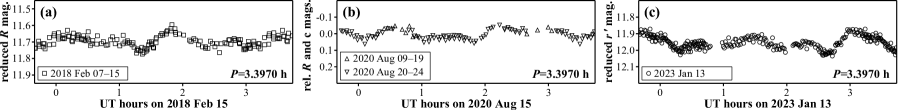
Figure 1: Composite lightcurves of (3032) Evans, light-time corrected and folded at 3.3970 h showing one period plus the earliest and latest 10% repeated. Legends give UT dates of observations. (a) 2018 apparition: The error in the $\mathit{R}$ mag. determined for the comparison star, based on observations with Landolt standard star SA097-249 (Landolt, 1992), is 0.007 mag. (b) 2020 apparition, August lunation. (c) 2023 apparition: Only the $\mathit{r^{\prime}}$ data are shown. The brightness zero-point is based on the comparison star’s catalog $\mathit{r^{\prime}}$ magnitude from the APASS DR10 catalog (Henden, 2019) with error 0.004 mag.

3 Resolving the period ambiguity

Slivan et al. (2018) identified three possible approaches for additional observations to identify the correct period:

Approach A: Test the previously unobserved viewing geometry for greater asymmetry in lightcurves. Earth-based observing geometries of Evans available during the years spanned by the lightcurves are clustered around four ecliptic longitudes roughly 90 degrees apart, three of which had been previously observed. The data from 2020 (Fig. 1b) represent the previously unobserved aspect, but the lightcurve shape asymmetry is smaller than that seen in 2008 and thus does not distinguish which period is correct.

Approach B: Lower-noise data near viewing geometry of greatest lightcurve asymmetry. The lightcurve from 2023 (Fig. 1c) records a lightcurve similar to that seen in 2008, and the use of a larger telescope at a dark site improves on the data quality and clearly establishes significant asymmetry in the lightcurve. Folding these data at the 1.7 h period thus rules out the doubly-periodic alias solution (Fig. 2), confirming that the correct rotation period is 3.4 h with quadruply-periodic lightcurves.

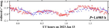
Figure 2: The same data as Fig. 1c but folded at 1.6985 h for a doubly-periodic lightcurve. The graph symbols distinguish in which half of rotation phase each data point would appear if it were folded at 3.3970 h instead. The significant difference in the subset lightcurves’ shapes between 1.1 h and 1.5 h in rotation phase indicates that this shorter period is not correct.

Approach C: Assemble a multi-apparition data set to determine the sidereal rotation period. The opportunity in 2023 to obtain data of high enough quality to resolve the synodic period ambiguity directly was unexpected. Even if instead the lightcurves had been of greater noise comparable to the previous observations, they still provide a sixth apparition of dedicated lightcurves for determination of the sidereal rotation period. This last approach to identifying the correct period distinguishes that the fractional rotations induced by angular changes in the direction vector affect the epochs differently in rotation phase depending on the rotation period. The approach is more powerful than the others because it does not depend on detecting asymmetry in the lightcurve shape, and motivates documenting the Evans analysis as a case study for reference.

4 Epochs analysis for sidereal rotations

The lightcurves reported in Sec. 2 were combined with published lightcurves of Evans (Slivan et al., 2018) for a data set comprising six apparitions spanning 15 years including all four available observing geometries, and satisfying the data set characteristics discussed by Slivan (2012, 2013).

The sidereal period of Evans is constrained by the time intervals between repeating lightcurve features, analyzed using the sieve algorithm described in detail by Slivan (2013). The approach identifies consistent sidereal rotation counts under the assumption that the epochs defining a given interval correspond to either the same asterocentric longitude or to reflex longitudes. It calculates the maximum possible fractional rotations induced by changes in the direction vector for both the prograde- and the retrograde-spin cases, making an approximation suitable for the small $3^{\circ}$ orbit inclination of Evans to calculate direction vector changes as the differences in ecliptic longitudes, but otherwise disregarding effects from changing polar aspect angle.

Complementing the sieve analysis for Evans is an RMS fit error noise spectrum analysis calculated using a model based on the same underlying assumptions, noting that the model requires that all of the epochs be referenced to the same time zero point, which is more restrictive than the sieve that depends only on the intervals between pairs of epochs. The spectrum calculation is a simplification of sidereal photometric astrometry (Drummond et al., 1988) limiting to the two equatorial aspect cases for prograde spin and retrograde spin, and without determining their corresponding pole ecliptic coordinates. Given $N$ epochs $t_{i}$ as time differences from the earliest epoch, the model is

$$t_{i}=Pn_{i}+\tau_{0}$$ (1)

where the fixed slope $P$ is a trial sidereal period and $\tau_{0}$ is the fitted intercept. The independent variable $n_{i}$ is the calculated number of elapsed sidereal rotations at epoch $t_{i}$:

$$n_{i}=0.5\mbox{ INT}\left[2\left(\frac{t_{i}}{P}\mp k_{i}\right)+0.5\right]\pm k_{i}$$ (2)

The maximum fraction of rotation $k_{i}$ induced by direction vector changes is calculated making the same approximation as is used for the sieve, by $k_{i}=\Delta\lambda_{i}/360^{\circ}$ where $\Delta\lambda_{i}$ is the angular difference of the PAB longitude for epoch $t_{i}$ from that for the earliest epoch. The signs of the $k_{i}$ in Eq. 2 depend on whether calculating for the asteroid spin direction that is the same as (upper signs) or opposite (lower signs) the orbit direction. For each trial period the least-squares solution for the model intercept is

$$\tau_{0}=\frac{1}{N}\left(\sum t_{i}-P\sum n_{i}\right)$$ (3)

where the sums are over the $N$ epochs, and the corresponding RMS error for the spectrum is

$$\sqrt{\frac{1}{N-1}\sum\left(t_{i}-(Pn_{i}+\tau_{0})\right)^{2}}$$ (4)

calculated for a series of trial sidereal periods over the range of the synodic period constraint. The separation of local minima (Kaasalainen et al., 2001, Eq. 2) informs the choice of period step size—for visual clarity a step of $0.1\times\left(P_{\rm syn}^{2}/2T\right)$ samples ten points per local minimum for synodic period $P_{\rm syn}$ and time span $T$ between the earliest and latest epochs.

4.1 Application to (3032) Evans

Table 3 summarizes the epochs used for the analyses, one selected per apparition, with their measurement errors $\sigma(t_{i})$ and the J2000.0 ecliptic longitude $\lambda_{\rm PAB}$ and latitude $\beta_{\rm PAB}$ of the corresponding phase angle bisectors. Epochs were measured from the composite lightcurves, in each case locating a maximum of the fourth harmonic of a Fourier series model fit to the lightcurves using the 3.397-h synodic rotation period as the fundamental. Despite the rather low amplitude, the lightcurves’ pattern of alternating brighter and fainter maxima is relatively symmetric in time, making it straightforward to choose an epoch corresponding to one of the brighter unfiltered maxima as suitable for analysis of both the doubly- and quadruply-periodic cases. The epoch measurement errors $\sigma(t_{i})$ are based on the RMS error of the corresponding unfiltered Fourier series fit model to the lightcurve data, calculating the corresponding error in time by dividing by the model’s steepest slope, on the brightness increase immediately preceding the brightest maximum.

Table 3: Epochs measured from the lightcurves.

UT date	Epoch (UT h)	$\lambda_{\rm PAB}$	$\beta_{\rm PAB}$	Ref.
2008 Jan 16	$0.34\pm 0.07$	$113.2^{\circ}$	$+1.7^{\circ}$	a
2009 May 11	$0.05\pm 0.07$	$192.0^{\circ}$	$+3.6^{\circ}$	a
2016 Nov 05	$2.26\pm 0.10$	$30.3^{\circ}$	$-3.4^{\circ}$	a
2018 Feb 15	$1.85\pm 0.05$	$126.5^{\circ}$	$+2.6^{\circ}$	b
2020 Aug 15	$0.55\pm 0.06$	$289.6^{\circ}$	$-1.9^{\circ}$	b
2023 Jan 13	$3.14\pm 0.03$	$132.9^{\circ}$	$+2.6^{\circ}$	b

Data references: (a) Slivan et al. (2018). (b) this work.

To avoid possible dependence of the analysis outcomes on the atypical lower noise of the 2023 lightcurve, an increased measurement error of 0.10 h was adopted for the 2023 epoch. Epoch range half-widths of $2.5\sigma(t_{i})$ were used for the sieve, and in a change from the description in Slivan (2013) the interval ranges were calculated from the epoch ranges as sums in quadrature. The synodic period constraint adopted as the test range of possible sidereal periods was $P_{\rm syn}\pm 2.5\sigma(P_{\rm syn})$.

Checking the quadruply-periodic case $P_{\rm syn}=3.3970\pm 0.0002$ h (Slivan et al., 2018) with the sieve algorithm identifies an unambiguous sidereal rotation count solution (Fig. 3a) that is insensitive to alternate choices of epoch range half-widths down to $1.0\sigma(t_{i})$, and is corroborated by the noise spectrum (Fig. 3b). The maximum interval between the 2008 and 2023 epochs corresponds to 38689 sidereal rotations, and the epochs are sufficient to distinguish that the spin is prograde.

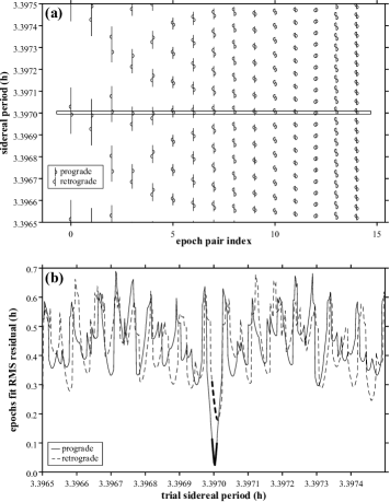
Figure 3: (a) Sieve algorithm identifies the sidereal period constraint for the quadruply-periodic case. Horizontal axis indices each represent the time interval between a pair of epochs, with longer intervals to the right. Semicircle symbols represent sidereal periods calculated from every possible number of rotations that could have elapsed during the interval, and vertical bars represent period ranges based on epoch range half-widths of $2.5\sigma(t_{i})$. The thin horizontal rectangle straddling 3.3970 h marks the single range of periods that is allowed by all fifteen time intervals. (b) RMS error spectrum for the quadruply-periodic case. Bold highlighting marks the allowed period range from the sieve algorithm Fig. 3a which contains the prograde RMS minimum at 3.39700 h.

Repeating the analysis but for the doubly-periodic case finds only unconvincing solutions whose existence is sensitive to the choice of epoch range half-widths (Fig. 4a); in fact, testing a reduction from $2.5\sigma(t_{i})$ to $1.0\sigma(t_{i})$ leaves no solutions at all (Fig. 4b). The noise spectrum has several indistinguishable local minima which also is not characteristic of correct solutions (Fig. 4c). The absence of a secure sidereal rotation count solution for 1.7 h, and the existence of the secure solution for 3.4 h, indicates that the 1.7 h period is an alias.

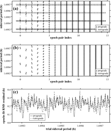
Figure 4: Similar to Fig. 3, but for the doubly-periodic case. (a) Sieve calculation using epoch range half-widths of $2.5\sigma(t_{i})$, for which the epoch pair at index 13 does not contribute a constraint and is not plotted. All of the allowed period ranges are sensitive to the half-widths as indicated by dashed markings. (b) Sieve calculation using epoch range half-widths of $1.0\sigma(t_{i})$, finding no allowed period ranges. (c) The fit error spectrum does not indicate a secure solution.

5 Analysis for spin vector and convex model

Having already resolved the true period from the alias, the remaining stages of spin vector and convex model analysis were carried out as described by Slivan et al. (2023). Comparably-weighting the lightcurve data by apparitions produced a lopsided distribution in aspect coverage; to aid the final convex inversion analyses the weighting was based on viewing aspects instead. Selected lightcurve fits are shown in Fig. 5. Spin vector results are summarized in Table 4: the derived sidereal period $P_{\rm sid}$ and its error, the symmetric pair of pole solutions’ J2000 ecliptic longitudes $\lambda_{0}$ and latitudes $\beta_{0}$, with their respective estimated errors $\sigma(\lambda_{0})$ and $\sigma(\beta_{0})$ in degrees of arc, the corresponding spin obliquities $\varepsilon$, and model shape axial ratios. The pole solutions satisfy the expected symmetry with respect to the “photometric great circle” (Magnusson et al., 1989; Slivan et al., 2023, Appendix A), but the $3^{\circ}$ orbit inclination of Evans is small enough to prevent distinguishing which is the true pole. The convex model shapes for the two symmetric poles are essentially mirror images of each other, to within their poorly-constrained scale factors in the direction along the polar axis. Renderings of one model are shown in Fig. 6, resembling a very rounded tetrahedral shape with its spin axis intersecting opposite edges.

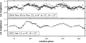
Figure 5: Selected model lightcurve fits with a pole $P_{{}_{2}}$ at (354^∘;$+$70^∘) as brightness vs. sidereal rotation phase. Legends give UT dates of the observations, solar phase angles $\alpha$, and sub-PAB latitudes $\theta$. The RMS error of the fit to the entire set of lightcurves corresponds to 0.021 mag.

Table 4: Spin vector results.

sidereal period $P_{\rm sid}$:	3.397003 $\pm$ 0.000002 h
	$\lambda_{0}$	$\sigma(\lambda_{0})$	$\beta_{0}$	$\sigma(\beta_{0})$	$\varepsilon$
spin poles $P_{{}_{1}}$:	186∘	5	$+$75∘	5	18∘
$P_{{}_{2}}$:	354∘	5	$+$70∘	5	17∘
model axial ratios:	$a/b$: 1.0a		$b/c$: 1.1a

Note (a) The axial ratios are very coarse estimates with uncertainties of at least $\pm 0.1$.

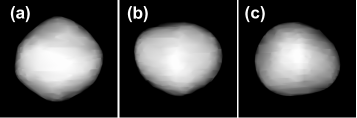
Figure 6: Renderings of convex model for pole $P_{{}_{2}}$. (a) Polar aspect showing the four-sided profile responsible for the quadruply-periodic lightcurves. (b,c) Equatorial aspects for the brighter and fainter pairs of lightcurve maxima, respectively.

6 Discussion and Conclusion

Observations and analysis reported in this work have resolved the factor of two ambiguity in the synodic rotation period of Koronis member (3032) Evans, confirming that its lightcurves are quadruply-periodic. The correct period was identified in two ways: first serendipitously by detecting asymmetry in an atypically high-quality lightcurve, and then deliberately by constraining the sidereal rotation period using the sieve algorithm of Slivan (2013) to analyze a suitable multi-apparition lightcurve data set. The latter approach can indicate the true period even for objects that do not show detectable asymmetry in their lightcurves’ shapes.

With its 3.4-h rotation period, Evans’s spin rate does not exceed the rubble-pile spin barrier (Pravec et al., 2002, Fig. 1) and thus presents no inconsistency with being a $\sim$14-km reaccumulated object member of the Koronis family.

Slivan et al. (2023) have discussed the Koronis member spin vector sample completed to $H$ $\sim$ 11.3, in which the smallest prograde-spinning objects also are the fastest prograde rotators and have low spin obliquities, consistent with having been spun up by YORP thermal radiation torques acting more quickly than on larger bodies (Rubincam, 2000). The spin vector properties of Evans are comparable to these spun-up prograde objects, noting that it is both smaller than and faster-rotating than they are.

Data Availability

Datasets related to this article can be found at http://smass.mit.edu/slivan/lcdata.html.

References

- Collins et al. (2017) Collins, K.A., Kielkopf, J.F., Stassun, K.G., Hessman, F.V., 2017. AstroImageJ: Image processing and photometric extraction for ultra-precise astronomical light curves. The Astronomical Journal 153, A77.
- Ditteon et al. (2018) Ditteon, R., Adam, A., Doyel, M., Gibson, J., Lee, S., Linville, D., Michalik, D., Turner, R., Washburn, K., 2018. Lightcurve analysis of minor planets observed at the Oakley Southern Sky Observatory: 2016 October–2017 March. Minor Planet Bulletin 45, 13–16.
- Drummond et al. (1988) Drummond, J.D., Weidenschilling, S.J., Chapman, C.R., Davis, D.R., 1988. Photometric geodesy of main-belt asteroids. II. Analysis of lightcurves for poles, periods, and shapes. Icarus 76, 19–77.
- Harris et al. (2014) Harris, A.W., Pravec, P., Gálad, A., Skiff, B.A., Warner, B.D., Világi, J., Gajdoš, Š., Carbognani, A., Hornoch, K., Kušnirák, P., Cooney, Jr., W.R., Gross, J., Terrell, D., Higgins, D., Bowell, E., Koehn, B.W., 2014. On the maximum amplitude of harmonics of an asteroid lightcurve. Icarus 235, 55–59.
- Henden (2019) Henden, A.A., 2019. APASS DR10 has arrived! The Journal of the American Association of Variable Star Observers 47, 130.
- Kaasalainen et al. (2001) Kaasalainen, M., Torppa, J., Muinonen, K., 2001. Optimization methods for asteroid lightcurve inversion. II. The complete inverse problem. Icarus 153, 37–51.
- Landolt (1992) Landolt, A.U., 1992. UBVRI photometric standard stars in the magnitude range 11.5 16.0 around the celestial equator. The Astronomical Journal 104, 340–371.
- Magnusson (1986) Magnusson, P., 1986. Distribution of spin axes and senses of rotation for 20 large asteroids. Icarus 68, 1–39.
- Magnusson et al. (1989) Magnusson, P., Barucci, M.A., Drummond, J.D., Lumme, K., Ostro, S.J., Surdej, J., Taylor, R.C., Zappalà, V., 1989. Determination of pole orientation and shapes of asteroids, in: Binzel, R.P., Gehrels, T., Matthews, M.S. (Eds.), Asteroids II. University of Arizona Press, Tucson, Arizona. chapter II, pp. 67–96.
- Narita et al. (2019) Narita, N., Fukui, A., Kusakabe, N., Watanabe, N., Palle, E., Parviainen, H., Montañés Rodríguez, P., Murgas, F., Monelli, M., Aguiar, M., Perez Prieto, J.A., Oscoz, A., de Leon, J., Mori, M., Tamura, M., Yamamuro, T., Béjar, V.J.S., Crouzet, N., Hidalgo, D., Klagyivik, P., Luque, R., Nishiumi, T., 2019. MuSCAT2: four-color simultaneous camera for the 1.52-m Telescopio Carlos Sánchez. Journal of Astronomical Telescopes, Instruments, and Systems 5, 015001.
- Pravec et al. (2002) Pravec, P., Harris, A.W., Michałowski, T., 2002. Asteroid rotations, in: Bottke, Jr., W.F., Cellino, A., Paolicchi, P., Binzel, R.P. (Eds.), Asteroids III. University of Arizona Press, Tucson, Arizona. chapter II, pp. 113–122.
- Rubincam (2000) Rubincam, D.P., 2000. Radiative spin-up and spin-down of small asteroids. Icarus 148, 2–11.
- Slivan (2012) Slivan, S.M., 2012. Epoch data in sidereal period determination. I. Initial constraint from closest epochs. Minor Planet Bulletin 39, 204–206.
- Slivan (2013) Slivan, S.M., 2013. Epoch data in sidereal period determination. II. Combining epochs from different apparitions. Minor Planet Bulletin 40, 45–48.
- Slivan et al. (2008) Slivan, S.M., Binzel, R.P., Boroumand, S.C., Pan, M.W., Simpson, C.M., Tanabe, J.T., Villastrigo, R.M., Yen, L.L., Ditteon, R.P., Pray, D.P., Stephens, R.D., 2008. Rotation rates in the Koronis family, complete to . Icarus 195, 226–276.
- Slivan et al. (2023) Slivan, S.M., Hosek, Jr., M., Kurzner, M., Sokol, A., Maynard, S., Payne, A.V., Radford, A., Springmann, A., Binzel, R.P., Wilkin, F.P., Mailhot, E.A., Midkiff, A.H., Russell, A., Stephens, R.D., Gardiner, V., Reichart, D.E., Haislip, J., LaCluyze, A., Behrend, R., Roy, R., 2023. Spin vectors in the Koronis family: IV. Completing the sample of its largest members after 35 years of study. Icarus 394, A115397.
- Slivan et al. (2018) Slivan, S.M., Neugent, K.F., Melton, C., Beck, M., 2018. Koronis family member (3032) Evans: Photometric reconnaissance and lightcurves in 2008, 2009, and 2016. Minor Planet Bulletin 45, 72–75.
- Taylor and Tedesco (1983) Taylor, R.C., Tedesco, E.F., 1983. Pole orientation of asteroid 44 Nysa via photometric astrometry, including a discussion of the method’s application and its limitations. Icarus 54, 13–22.