On the geography of $3$-folds via asymptotic behavior of invariants

Abstract.

Roughly speaking, the problem of geography asks for the existence of varieties of general type after we fix some invariants. In dimension $1$, where we fix the genus, the geography question is trivial, but already in dimension $2$, it becomes a hard problem in general. In higher dimensions, this problem is essentially wide open. In this paper, we focus on geography in dimension $3$. We generalize the techniques which compare the geography of surfaces with the geography of arrangements of curves via asymptotic constructions. In dimension $2$ this involves resolutions of cyclic quotient singularities and a certain asymptotic behavior of the associated Dedekind sums and continued fractions. We discuss the general situation with emphasis on dimension $3$, analyzing the singularities and various resolutions that show up, and proving results about the asymptotic behavior of the invariants we fix.

1. Introduction

We work with normal projective varieties $X$ over the complex numbers ${\mathbb{C}}$. As usual, when $\dim X=1$, $2$, or $d\geq 3$ we say that $X$ is a curve, a surface, or a $d$-fold respectively. A central problem in algebraic geometry is to classify varieties of general type, i.e., varieties with positive canonical volume ${\mbox{vol}}(X)$. By definition

$$\mbox{vol}(X)=\limsup_{m\to\infty}\frac{h^{0}(X,mK_{X})}{m^{d}/d!},$$

where $d=\dim X$, and $K_{X}$ is the Weil divisor associated with the dualizing sheaf. It is called the canonical divisor of $X$.

Nowadays and because of the minimal model program, we can always reduce our problem to classify minimal/canonical models of birational classes [BCHM10]. A first step is the problem of geography. After we agree on some numerical invariants, this means: Given a collection of numbers, is there a minimal/canonical variety of general type whose numerical invariants are equal to that collection of numbers? Furthermore, by the existence of the KSBA compactifications of moduli spaces (see [KSB88], [Ale94], [Kol23]), we are interested in a wider geography problem for varieties of general type with ($\log$) terminal/canonical singularities with nef/ample canonical bundle.

In dimension one, the main invariant is the genus $g$. If $X$ is a non-singular curve of general type, then we have

$$\mbox{vol}(X)=\deg K_{X}=-2\chi({\mathcal{O}}_{X})=-e(X)=2g-2>0\Leftrightarrow g\geq 2.$$

Thus, the geography problem asks: Given an integer $g\geq 2$, is there a curve of genus $g$? This can be easily answered. Indeed, for example, one can construct curves for any $g\geq 2$ as double covers of ${\mathbb{P}}^{1}$ branched at $2g+2$ points.

In dimension two the problem is much harder. In order to choose invariants, the Riemann-Roch theorem suggests that, for any surface $X$, one can pick the top-intersection of the canonical class $K_{X}^{2}$, and the analytical Euler characteristic $\chi({\mathcal{O}}_{X})$. When $X$ is non-singular, we have the Noether’s formula $K^{2}_{X}+e(X)=12\chi({\mathcal{O}}_{X})$. These two invariants $K_{X}^{2},\chi({\mathcal{O}}_{X})$ are equivalent to the two Chern numbers $c_{1}^{2}(X)=K_{X}^{2}$, and $c_{2}(X)=e(X)$. If we fix our attention to minimal surfaces of general type, then the geography problem asks: Given $(a,b)\in{\mathbb{Z}}^{2}$, is there a minimal surface $X$ such that $c_{1}^{2}(X)=a$, and $c_{2}(X)=b$? A pioneer in this question (and the creator of the term “geography") was Ulf Persson [Per81]. He proved the existence of minimal surfaces of general type $X$ with $c_{1}^{2}(X)=a$, $c_{2}(X)=b$ satisfying $\frac{b-36}{5}\leq a\leq 2b$ with $2a\neq b-k$, where $k=2$, or $k$ is odd with $1\leq k\leq 15$ or $k=19$. A more general result was obtained in [Che87] and [Che91]. (It is still an open problem to realize every point.)

As we just saw, working on the geography problem for pairs of Chern numbers in the non-compact region $c_{1}^{2},c_{2}>0$ (General type inequality), $5c_{1}^{2}-c_{2}+36\geq 0$ (Noether’s inequality [Noe75]), and $c_{1}^{2}\leq 3c_{2}$ (BMY-inequality [Bog78, Miy77, Yau77]) could be cumbersome. We can weaken the problem considering Chern slopes $c_{1}^{2}/c_{2}$. Somesse [Som84] proves that any rational number in $[1/5,3]$ is realized as $c_{1}^{2}(X)/c_{2}(X)$ by a minimal surface of general type $X$, answering a question asked by Hirzebruch in [Hir83, (3.3)]. In particular, there are no “not-allowed-holes" in $[1/5,3]$. The surfaces constructed by Sommese have no control over other invariants, for example, their fundamental group. One could ask: How do the slopes of minimal surfaces of general type with fixed fundamental group distribute in $[1/5,3]$? The results of [RU15] and [TU22] prove that if $G$ is the fundamental group of a surface, then the Chern slopes of minimal surfaces of general type with $\pi_{1}$ isomorphic to $G$ are dense in $[1,3]$ .

In dimensions greater than or equal to $3$, we know dramatically less about their geography. At least we have the existence of moduli spaces for KSBA-stable models for each dimension. A comprehensive treatment can be found in [Kol23]. Since in higher dimensions, our minimal models may admit singularities, we do not have directly the notion of Chern numbers. If $X$ is a non-singular $3$-fold, then we have Chern numbers

$$c_{1}^{3}(X)=-K_{X}^{3},\quad c_{1}c_{2}(X)=24\chi({\mathcal{O}}_{X}),\quad c_{3}(X)=e(X).$$

For $X$ a minimal non-singular $3$-fold we have a Noether’s type inequality [CH06],

$$c_{1}^{3}(X)\leq\frac{1}{27}c_{1}c_{2}(X)+\frac{10}{3}.$$ (1)

When $X$ is singular, we consider as invariants for our geography problem: $K_{X}^{3}$, $\chi({\mathcal{O}}_{X})$, and $e(X)$. As in the case of surfaces, we also have some inequalities for them. If $X$ is minimal of general type, then we have $K_{X}^{3}>0$. In [Hu18], it was proved the Noether’s type inequality for Gorenstein minimal $3$-folds of general type:

$$-K_{X}^{3}\leq\frac{4}{3}\chi({\mathcal{O}}_{X})+2.$$

We also have the Miyaoka-Yau inequality for Gorenstein minimal $3$-folds of general type [Miy87],

$$-K_{X}^{3}\geq 72\chi({\mathcal{O}}_{X}),$$

with equality if and only if $X$ is a ball quotient. In [GKPT19], it was proved a ${\mathbb{Q}}$-version of Miyaoka-Yau inequality, i.e., a similar inequality when $X$ is a projective Kawamata log-terminal $3$-fold of general type with nef canonical divisor. In the previous two inequalities above, the results were written in terms of $K_{X}^{3}$ and $\chi(\omega_{X})$. However, since we are restricting ourselves to the Gorenstein case, we have $\chi(\omega_{X})=-\chi({\mathcal{O}}_{X})$.

From the birational geometry of $3$-folds, the triple $(K_{X}^{3},\chi({\mathcal{O}}_{X}),e(X))\in{\mathbb{Q}}\times{\mathbb{Z}}^{2}$ is invariant between minimal models of the same birational class. Indeed, two minimal models in the same birational class are isomorphic in codimension $1$ [Mat10, 12.1.2]. Therefore $K_{X}^{3}$ is an invariant. Minimal models are connected by flops, and they are surgeries reversing the orientation of some $K$-trivial rational curves. Thus flops leave invariant the numbers $h^{i}({\mathcal{O}}_{X})$ and $h^{i}(X,{\mathbb{Z}})$ for each $i$ [Kol91, Th.3.2.2].

The main purpose of this paper is to study the geography problem for $3$-folds of general type. We can state the geography problem as follows: Given a triple $(a,b,c)\in{\mathbb{Q}}\times{\mathbb{Z}}^{2}$ satisfying the restrictions above, is there a $3$-fold of general type $X$ such that $(-K_{X}^{3},\chi({\mathcal{O}}_{X}),e(X))=(a,b,c)$? We can distinguish two cases:

• Geography for minimal $3$-folds with terminal singularities, in the realm of canonical models.

• Geography for minimal $3$-folds with log-terminal singularities, in the realm of KSB-stable models.

For minimal $3$-folds $X$ of general type, $\chi({\mathcal{O}}_{X})$ and $e(X)$ could be negative, positive or zero. In [Hun89] was proposed the study of slopes

$$[c_{1}^{3},c_{1}c_{2},c_{3}]\in{\mathbb{P}}^{2}_{{\mathbb{Q}}}$$

for non-singular minimal models, extending naturally to the singular case by taking slopes $[-K_{X}^{3},\chi({\mathcal{O}}_{X}),e(X)]\in{\mathbb{P}}^{2}_{{\mathbb{Q}}}$. This, allows us to work by charts. Indeed, in [Hun89], the author studied slopes of non-singular $3$-folds with ample canonical class in the chart $c_{1}c_{2}\neq 0$. Moreover, since $\chi({\mathcal{O}}_{X})<0$ for Gorenstein minimal models of general type, we consider that as the chart of study.

The first question that one can ask is: Do those slopes lie in a bounded region? Observe that all inequalities above just bound the coordinate $c_{1}^{3}/c_{1}c_{2}$. In [CL01] is proved that the Chern slopes $[c_{1}^{3},c_{1}c_{2},c_{3}]$ of non-singular $3$-folds with ample canonical bundle define a bounded region by finding inequalities for the coordinate $c_{3}/c_{1}c_{2}$. However, this bound is not optimal. In a more general setup, let $N(d)$ be the number of partitions of $d$. In [DS22], it is proved that Chern slopes $[c_{1}^{d},\ldots,c_{d}]\in{\mathbb{P}}^{N(d)-1}_{{\mathbb{Q}}}$ of non-singular $d$-folds with ample canonical bundle define a bounded region in the chart $c_{1}^{d}\neq 0$.

To illustrate the case of $3$-folds, in Figure 1 we see the map in chart $c_{1}c_{2}\neq 0$ for minimal non-singular $3$-folds of general type. In the rest, we describe the zones on that map.

• Allowed zone: This is the region bounded by the Miyaoka-Yau inequality $c_{1}^{3}/c_{1}c_{2}\leq 8/3$ and $c_{1}^{3}/c_{1}c_{2}>0$. They are sketched by black lines.

• Noether’s line: Since $\chi({\mathcal{O}}_{X})<0$ is an integer, we can avoid small values of this invariant. Thus, from the Noether’s inequality (1), $3$-folds with $|c_{1}c_{2}|\gg 0$ must satisfy $c_{1}^{3}/c_{1}c_{2}\geq 1/27$. Thus, the Noether’s line is the red line defined by $c_{1}^{3}/c_{1}c_{2}=1/27$.

• Cartesian Product Zone (CP line): The zone CP collects $3$-folds of the form $S\times C$ for surface $S$ and a curve $C$ both with ample canonical bundle (see Example 2.2). The Chern slopes $(c_{1}^{3}/c_{1}c_{2},c_{3}/c_{1}c_{2})$ of these $3$-folds distribute densely along the line in ${\mathbb{A}}^{2}$ connecting the points $(9/4,1/4)$ and $(1/2,5/6)$. This is the purple line on the map.

• $3$-folds in ${\mathbb{P}}^{4}$ and ${\mathbb{P}}^{5}$. The minimal non-singular $3$-folds of general type in ${\mathbb{P}}^{4}$ are hypersurfaces of degree $d>5$. Its Chern classes are explicitly exhibited in Section 5.2. The Chern slopes have the form

  $$\frac{c_{1}^{3}}{c_{1}c_{2}}=\frac{d^{3}-15d^{2}+75d-125}{d^{3}-10d^{2}+35d-50},\quad\frac{c_{3}}{c_{1}c_{2}}=\frac{d^{3}-5d^{2}+10d-10}{d^{3}-10d^{2}+35d-50}.$$

  So, their slopes $(c_{1}^{3}/c_{1}c_{2},c_{3}/c_{1}c_{2})$ are asymptotically near to $(1,1)$ as $d$ grows. On the map, they are sketched with blue points. In [Cha99] was proved that $3$-folds embedded in ${\mathbb{P}}^{5}$ whose canonical class $K$ satisfy $K^{i}H^{j}>0$ for a hyperplane section, distribute along the line defined by

  $$x+y=2,\quad 1\leq x\leq 2.$$

  We sketch it on the map with a blue line.

• Smooth Complete Intersection Zone (SCI): The zone SCI collects non-singular complete intersections with ample canonical sheaf. In [Cha97] it is proved the existence of an optimal region for which we have density. This region is sketched with orange color on the map. The problem with this region is that it not contains all SCI $3$-folds. The remainder is distributed discretely outside that region. However, in [SXZ14] was proved that the convex closure of the slopes $(c_{1}^{3}/c_{1}c_{2},c_{3}/c_{1}c_{2})$ for SCI $3$-folds is a rational polyhedron with infinitely many faces. The main vertices of this polyhedron are $(1/16,43/8)$ and $(2,1/3)$. The region described in this theorem is sketched with the color yellow on the map.

• Zone Fermat: Using the basic construction of Fermat covers, in [Hun89, Th. 8.2.1 and Th.8.2.2] was proved that there exists triangles $\Delta ABC$ in ${\mathbb{Q}}^{2}$ such that for every $(a,b)\in\Delta ABC$ there exists a smooth projective $3$-fold $X$ with ample canonical bundle such that,

  $$\left(\frac{c_{1}^{3}(X)}{c_{1}c_{2}(X)},\frac{c_{3}(X)}{c_{1}c_{2}(X)}\right)=(a,b).$$

  It was found two large triangles with vertices

  $$A=(12/11,1/11),B=(6/5,3/5),C=(41/33,19/33),$$

  $$A=(1,-2/5),B=(1,2/3),C=(32/29,55/87).$$

  They are sketched by light green triangles on the map. This technique was improved in [Liu97]. The regions constructed are sketched with green.

• Isolated points: The isolated gray points show minimal non-singular $3$-folds constructed by Fermat over arrangements of hyperplanes, and desingularizations of complete intersection. In this case, we have examples for $c_{3}>0$ [Hun89, Section 7.3]. We sketch two of these points

  $$(1.4,-0.22)\quad\text{ Fermat cover over }CEVA^{3}(2),$$

  $$(0.83,-0.125),\quad\text{ Resolution of complete intersection $(5,5)$ in ${\mathbb{P}}^{5}$ }.$$

• Ball quotient point: The Miyaoka-Yau inequality asserts that every non-singular $3$-fold with ample canonical bundle satisfying $c_{1}^{3}=\frac{8}{3}c_{1}c_{2}$ is a smooth ball quotient. By Hirzebruch proportionality [Hir58] a ball quotient must satisfy $c_{3}/c_{1}c_{2}=\frac{1}{6}$. This implies that all non-singular varieties with ample canonical bundle and equating the Miyaoka-Yau inequality lie in only one point, i.e., $(8/3,1/6)$.

• Unknown Zone: We define the unknown zone as the region over the SCI yellow region and over the extension of the CP line from the point $(2,1/3)$. The emptiness of this zone was conjectured by Hunt in [Hun89], and the author do not know about the existence of minimal non-singular $3$-folds with such slopes. See Section 6.3 for explicit description.

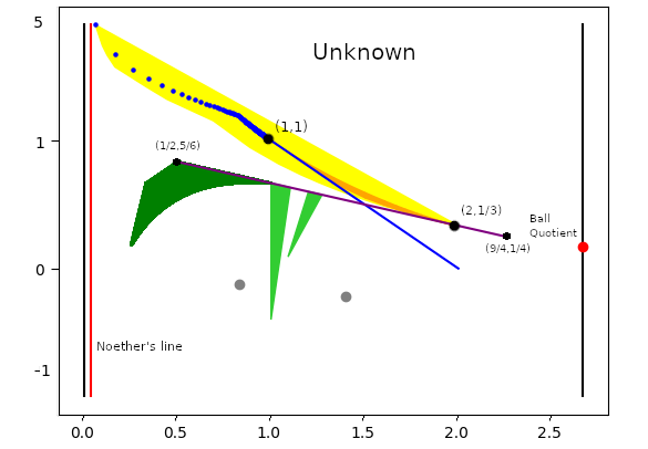
Figure 1. The map in coordinates $(c_{1}^{3}/c_{1}c_{2},c_{3}/c_{1}c_{2})$ for minimal non-singular $3$-folds of general type. The $y$-axis is scaled to show the complete picture.

1.1. Results of this work

When working with slopes, it turns out that we can apply the tool of $n$-th root coverings to investigate their behavior. Although it is not a straightforward result for dimensions $2$ or more, in dimension $1$ it is easy to see this phenomenon.

Consider the following data. Let $Z$ be a non-singular projective variety of dimension $d$, and let $D_{1},\ldots,D_{r}$ be distinct prime divisors in $Z$. Assume that $D_{red}:=D_{1}+\ldots+D_{r}$ is a simple normal crossing divisor (SNC). Let $n>1$ be a positive integer, and let $0<\nu_{i}<n$ be a collection of $r$ integers coprime to $n$. Assume that there exists a line bundle ${\mathcal{L}}$ on $Z$ such that

$${\mathcal{L}}^{\otimes n}\simeq{\mathcal{O}}_{Z}\left(\sum_{i=1}^{r}\nu_{i}D_{i}\right).$$ (2)

Then, there exists an $n$-th root cover $h_{n}\colon Y_{n}\to Z$ branched along $D_{red}$, where $Y_{n}$ is a normal projective variety (Section 2.2). These are the $n$-th root covers developed by Esnault and Viehweg in [Esn82], [Vie82] (Cf. [EV92]). For curves, the prime divisors $D_{1},\ldots,D_{r}$ are distinct points on $Z$, and the existence of such ${\mathcal{L}}$ is equivalent to $\sum_{i=1}^{r}\nu_{i}\equiv 0$ modulo $n$. Moreover, since points are isolated, we have $Y_{n}$ as a non-singular curve. By the Riemann-Hurwitz formula, we have

$$\frac{c_{1}(Y_{n})}{n}=\frac{nc_{1}(Z)-(n-1)r}{n}=c_{1}(Z)-r+\frac{r}{n}=\bar{c}_{1}(Z,D_{red})+\frac{r}{n}.$$

Here $\bar{c}_{1}(Z,D_{red})$ is the first logarithmic Chern number of the pair $(Z,D_{red})$ (see Section 2.1). Hence, if we fix the points $D_{red}$ and we consider partitions $\nu_{1}+\ldots+\nu_{r}=n$ with $n\gg 0$ a prime number, then we asymptotically have $c_{1}(Y_{n})\approx n\bar{c}_{1}(Z,D_{red})$.

Question 1.1.

Does this asymptotic phenomenon happen in higher dimensions?

In Section 3, we prove that this phenomenon occurs in general when the branch locus is a disjoint collection of non-singular distinct prime divisors $D_{1},\ldots,D_{r}$. In this case, as above, we have $Y_{n}$ as a non-singular projective variety, and it is independent of the multiplicities $\nu_{i}$.

Theorem A.

Assume we have $n$-th root covers $h\colon Y_{n}\to Z$ branched at $D=\sum_{j}\nu_{j}D_{j}$. If $D_{red}$ is non-singular, then for each partition $i_{1}+\ldots+i_{m}=d$, the Chern numbers satisfy,

$$\frac{c_{i_{1}}\ldots c_{i_{m}}(Y_{n})}{n}\approx\bar{c}_{i_{1}}\ldots\bar{c}_{i_{m}}(Z,D),$$

for prime numbers $n\gg 0$.

However, this theorem is restrictive for us in terms of geography. It is difficult to get the necessary hypothesis to construct a minimal $d$-fold of general type. See Section 3.2. On the other hand, we do not drop the possibility of having applications in other contexts. See Example 3.5. Also, this is a cornerstone of our research and opens the following discussion.

For $\dim Z\geq 2$, if the branch divisor $D_{red}=D_{1}+\dots+D_{r}$ has singularities, then $Y_{n}$ have rational singularities [Vie77]. In order to have well-behaved invariants, we can choose a (partial) resolution of singularities. For $\dim Z=2$, the asymptoticity of Chern numbers was proved in [Urz09] for random $n$-th root covers. Let us explain briefly what random means (see Section 2.3 for more details). First, in dimension two, each singularity of $Y_{n}$ is a cyclic surface singularity of type $\frac{1}{n}(q,1)$ for some $0<q<n$. Thus, we use the Hirzebruch-Jung algorithm (see Section 7.1) to resolve these singularities in a minimal way. For us, there are two important quantities, (1) the length of the resolution, i.e., the number of steps of the algorithm, and (2) the Dedekind sums,

$$d(q,1,n)=\sum_{i=1}^{n-1}\left(\left(\frac{iq}{n}\right)\right)\left(\left(\frac{i}{n}\right)\right),$$

where $((\cdot)):{\mathbb{R}}\to{\mathbb{R}}$ is the saw-tooth function (see Section 7.2). We get a resolution of singularities $X_{n}\to Y_{n}$. However, the Chern numbers $c_{1}^{2}$ and $c_{2}$ depend on the lengths and the Dedekind sums coming from all cyclic singularities resolved. To guarantee asymptoticity, we have to consider asymptotic arrangements. Indeed, for each prime number $n\geq 17$, there exists a set $O_{n}\subset\{1,\ldots,n\}$ (Section 2.3) such that for each $q\in O_{n}$, the lengths and Dedekind sums are bounded by $c\sqrt{n}$ for a constant $c>0$. Thus we say that $D_{red}$ is an asymptotic arrangement if satisfies :

• For prime numbers $n\gg 0$, there exists multiplicities $0<\nu_{j}<n$ such that the singularity over $D_{j}\cap D_{k}$ of $Y_{n}$ is of type $\frac{1}{n}(q_{jk},1)$ with $q_{jk}\in O_{n}$.

• For each $n$ there are line bundles ${\mathcal{L}}\in\mbox{Pic}(Z)$ such that

  $${\mathcal{L}}^{\otimes n}\simeq{\mathcal{O}}_{Z}\left(\sum_{j=1}^{r}\nu_{j}D_{j}\right).$$

The main set-up is when there exists $H\in\mbox{Pic}(Z)$ such that $D_{j}\simeq H$ for each component of $D_{red}$. Observe that the condition (2) is satisfied as

$$D=\nu_{1}D_{1}+\ldots+\nu_{r}D_{r}\sim(\nu_{1}+\ldots+\nu_{r})H\sim nH,$$

thus we can construct $n$-th root covers. In [Urz09] was proved that for a random partition $\nu_{1}+\ldots+\nu_{r}=n$, the probability of $D$ being an asymptotic arrangement tends to $1$ as $n$ grows. In this way, for $n\gg 0$ we take random asymptotic partitions, and we get a family of random surfaces $X_{n}$ with

$$c_{1}^{2}(X_{n})\approx n\bar{c}_{1}^{2}(Z,D_{red}),\quad c_{2}(X_{n})\approx n\bar{c}_{2}(Z,D_{red}).$$

Now we can discard the SNC property for the branch divisor. We consider a $\log$ resolution $\gamma\colon Z^{\prime}\to Z$ such that the reduced divisor defined by $\gamma^{*}D_{red}$ is SNC (2.31). If such a divisor turns out to be an asymptotic arrangement, then we have the asymptotic result for Chern numbers as above. See Theorem 2.32 in Section 2.3 or [Urz16] in order to connect this result with minimal models. A direct application is a relation between Chern slopes of simply-connected surfaces of general type and Chern slopes of arrangements of lines [EFU22]. In this way, in higher dimensions, we have several issues to achieve an analog asymptotic result. For example, the singularities of $Y_{n}$ are not cyclic, and the choice of a right (partial) resolution of $Y_{n}$ with good behavior as $n$ grows is a challenging problem.

Question 1.2.

Is there an analog of the asymptotic results in dimension two for dimension three?

For instance, if this question has a positive answer, then we would be able to study the geography of $3$-folds using arrangements of planes in ${\mathbb{P}}^{3}$. The first result in this direction is in Section 4.1, where we find that the Chern number $c_{1}c_{2}=24\chi$ is asymptotic and independent of the chosen resolution. However, the volume and the topological characteristic depend on the chosen resolution. As above, we may be interested in a $\log$-geography. In this way, the singularities of $Y_{n}$ are $\log$-terminal, however of multiplicity $n^{2}$, too big. This means that in order to connect with a non-singular model, at a bad choice of resolution we could have big exceptional data with respect to $n$, and so we would lose the asymptoticity of invariants at least topologically. In Section 4.2, we introduce a prototype of first step, i.e., by toric methods we construct a local cyclic resolution . In this way, we get singularities of multiplicity lower than $n$, and of cyclic quotient type. We are interested in cyclic quotient singularities since they are $\log$-terminal and have a well-known algorithm to resolve them: the Fujiki-Oka continuous fraction (Cf. [Ash19]). In Section 4.3 we globalize this local cyclic resolution, and we get a cyclic resolution $X_{n}\to Y_{n}$. It is important to note that it is an embedded ${\mathbb{Q}}$-resolution in the language of [ABMMOG12], introduced as an efficient resolution without useless data. We summarized the work of that section in the next theorem.

Theorem B.

Let $Z$ be any non-singular projective $3$-fold, and let $\{D_{1},\ldots,D_{r}\}$ be an asymptotic arrangement. For prime numbers $n\gg 0$ there are projective $3$-folds $X_{n}\to Z$ with at most cyclic quotient singularities such that

$$\frac{-K_{X_{n}}^{3}}{n},\frac{24\chi({\mathcal{O}}_{X_{n}})}{n},\frac{e(X_{n})}{n}\approx\bar{c}_{1}^{3}(Z,D),\bar{c}_{1}\bar{c}_{2}(Z,D),\bar{c}_{3}(Z,D),$$

where $\bar{c}_{i}(Z,D)$ are the Chern classes of the arrangement.

This result can be extended to an arbitrary collection of surfaces ${\mathcal{A}}=\{D_{1},\ldots,D_{r}\}$ having only simple crossing, i.e., each $D_{j}$ is non-singular, pairwise intersections are transversal, and components of $D_{j_{1}}\cap\ldots\cap D_{j_{e}}$ are non-singular. In 2.31 we use a $\log$-resolution $Z^{\prime}\to Z$ to get a SNC arrangement which results to be asymptotic if ${\mathcal{A}}$ is. Therefore, we can apply again B. See Example 2.33.

Finally, with these constructions: What can we say about geography of $3$-folds of general type? As an application of the above theorem to the geography of $3$-folds, we have two results about the behavior of the slopes of invariants. In Section 5 we see our resolution in terms of pairs $(X_{n},\tilde{D}_{red})\to(Z,D_{red})$. As a corollary, we prove that for asymptotic arrangements of hyperplane sections on a minimal $3$-fold of general type, the resolution preserves the bigness of the $log$-canonical divisor $K_{X_{n}}+\tilde{D}_{red}$.

Corollary 1.3.

Let $Z\hookrightarrow{\mathbb{P}}^{d}$ be a minimal non-singular projective $3$-fold of general type, and let $\{H_{1},\ldots,H_{r}\}$ be a collection of hyperplane sections in general position. Then, for prime numbers $n\gg 0$ there are finite morphisms of degree $n$ $(X_{n},\tilde{D}_{red})\to(Z,D_{red})$ such that:

1. $X_{n}$ is of $\log$-general type, i.e., $K_{X_{n}}+\tilde{D}_{red}$ is big and nef,

2. $K_{X_{n}}^{3}>0$,

3. $X_{n}$ has cyclic singularities ($\log$-terminal) of order lower than $n$, and

4. the slopes $(-K^{3}/24\chi,e/24\chi)$ of $X_{n}$ are arbitrarily near to $(2,1/3)$.

The importance of this theorem is: We are in the realm of $\log$-minimal models, and the existence of a non-singular model depends on resolving cyclic quotient singularities of order $n$. We point out that $K_{X_{n}}^{3}>0$, so in future work, if we are able to control the MMP of the chosen resolution, then we will have the asymptotic results with $K_{X_{n}}$ nef, so for $n\gg 0$, the varieties $X_{n}$ will be of general type. For us, the goal is that the asymptotic behavior of the slopes of $X_{n}$ coincides with the slopes of its minimal models (see Theorem 2.32). For this, we need a good terminalization of the cyclic singularities obtained. In Section 6 we discuss what means the word good.

In Section 5.2, choosing a similar path as for B, we construct minimal non-singular $3$-fold of general type using as a base $3$-folds $Z\hookrightarrow{\mathbb{P}}^{4}$ with $3$ hyperplane sections. So, we get almost asymptoticity of the volume. This means that with respect to $n\gg 0$ the volume converges to $c_{1}^{3}(Z,D)$ plus another finite quantity. However, this allows us to prove.

Theorem C.

For $d>5$ and prime numbers $n\gg 0$ there are projective minimal non-singular $3$-folds $X_{n}$ of general type having over $Z$ with slopes

$$\frac{c_{1}^{3}}{c_{1}c_{2}}\approx\frac{(d-2)^{3}-1}{(d-2)(d-1)^{2}},\quad\frac{c_{3}}{c_{1}c_{2}}\approx\frac{(d-5)(d^{2}+2d+6)}{(d-2)(d-1)^{2}}.$$

In particular, as the degree of $Z$ grows, the slopes have limit point $(1,1)$.

We obtain a new map in Figure 2. The reader can observe the position of the point $(2,1/3)$ where cyclic resolutions along hyperplane section arrangements accumulate. Indeed, this is on the border of the Unknown Zone. See discussion in Section 6.3. The slopes of C are inside of a parameterized curve accumulating at $(1,1)$ defining new points on the map. Finally, in Section 6 we discuss the future of this work.

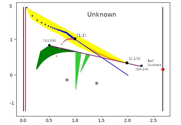
Figure 2. Map after this work. The parameterized curve of color contains minimal non-singular $3$-folds of general type with slopes arbitrarily near to $(1,1)$.

Acknowledgments: I am grateful to my Ph.D. thesis advisor Giancarlo Urzúa for his time, guidance, and support throughout this work. The results in this paper are part of my Ph.D. thesis at the Pontificia Universidad Católica de Chile. I would also like to thank Jungkai Alfred Chen for his hospitality during my stay at the National Center for Theoretical Sciences in Taiwan. Special thanks to Pedro Montero and Maximiliano Leyton, for many comments and suggestions to improve this work. I was funded by the Agencia Nacional de Investigación y Desarrollo (ANID) through the Beca Doctorado Nacional 2019.

2. Preliminaries

2.1. Logarithmic properties

For a non-singular projective variety $Z$ of dimension $d$ over ${\mathbb{C}}$, let $A(Z)=\bigoplus_{e\geq 0}A^{e}(Z)$ be its Chow ring, where $A^{e}(Z)$ are the Chow groups of $e$-cycles. We denote its Chern classes by $c_{e}(Z)\in A^{e}(Z)$, i.e. the Chern classes of its tangent bundle ${\mathcal{T}}_{Z}$ [Har77, Appendix A]. We have that $c_{1}(Z)=-K_{Z}$, where $K_{Z}$ is the canonical class. We define the Chern numbers of $Z$ as the degree of the top-intersection of its Chern classes

$$c_{i_{1}}(Z)\ldots c_{i_{m}}(Z)\in A^{d}(Z),\quad i_{1}+\ldots+i_{m}=d.$$

In the following, if the context is understood, we abuse notation using the symbol $c_{i_{1}}\ldots c_{i_{m}}(Z)$ for Chern numbers. Also, we may use the notation $c_{i_{1}}\ldots c_{i_{m}}$.

We have $c_{1}^{d}=(-1)^{d}K_{Z}^{d}$, and since we work over ${\mathbb{C}}$, it is well-known that $c_{d}=e(Z)$, the topological Euler characteristic. These numbers are codified into the Todd class of ${\mathcal{T}}_{Z}$ by the following formal sum

$$\mbox{td}({\mathcal{T}}_{Z})=1+\frac{c_{1}}{2}+\frac{c_{1}^{2}+c_{2}}{12}+\frac{c_{1}c_{2}}{24}-\frac{c_{1}^{4}-4c_{1}^{2}c_{2}-3c_{2}^{2}-c_{1}c_{3}+c_{4}}{720}+\ldots.$$

As a consequence of the Hirzebruch-Riemann-Roch Theorem, we have the Noether’s identities, i.e., the analytic Euler characteristic are equal to the $d$-th summand of $\mbox{td}({\mathcal{T}}_{Z})$. For example

$$\chi({\mathcal{O}}_{Z})=\dfrac{c_{1}c_{2}}{24},\quad\text{when }d=3.$$

Let us construct some examples using just fiber products. Consider a collection $Z_{1},\ldots,Z_{s}$ of non-singular projective varieties. Set $Z=Z_{1}\times\ldots\times Z_{s}$, and $p_{i}\colon Z\to Z_{i}$ the corresponding projections. We have ${\mathcal{T}}_{Z}=\bigoplus_{i=1}^{s}p_{i}^{*}{\mathcal{T}}_{Z_{i}}$, and so in terms of Chern polynomials we can compute

$$c_{t}({\mathcal{T}}_{Z})=\prod_{i=1}^{s}p_{i}^{*}c_{t}({\mathcal{T}}_{Z_{i}}).$$

The following is deduced via routine computations.

Proposition 2.1.

Consider $Z=Z_{1}\times Z_{2}$ with $\dim Z_{i}=d_{i}$. Then for any partition $i_{1}+\ldots+i_{m}=d_{1}+d_{2}$ we have

$$c_{i_{1}}\ldots c_{i_{m}}(Z)=\sum_{\begin{subarray}{c}k_{j}+l_{j}=i_{j}\\ k_{1}+\ldots+k_{m}=d_{1}\\ l_{1}+\ldots+l_{m}=d_{2}\end{subarray}}c_{k_{1}}\ldots c_{k_{m}}(Z_{1})c_{l_{1}}\ldots c_{l_{m}}(Z_{2}).$$

In particular, the topological Euler characteristic satisfy $e(Z)=e(Z_{1})e(Z_{2})$.

∎

Example 2.2.

Let $C$ be a non-singular curve and $V$ any non-singular projective variety of dimension $d$. Set $Z=V\times C$. From the above formula and for any partition $i_{1}+\ldots+i_{m}=d+1$, we get

$$c_{i_{1}}\ldots c_{i_{m}}(Z)=\left(\sum_{j=1}^{m}c_{i_{1}}\ldots c_{i_{j}-1}\ldots c_{i_{m}}(V)\right)e(C).$$

In particular, $c_{1}^{d+1}=dc_{1}^{d}(V)e(C)$. If $V$ is a surface, then $Z$ is a $3$-fold with

$$c_{1}^{3}=3K_{V}^{2}e(C),\quad c_{1}c_{2}=12\chi({\mathcal{O}}_{V})e(C),\quad c_{3}=e(V)e(C).$$

Then in terms of slopes, we have

$$\left(\frac{c_{1}^{3}}{c_{1}c_{2}},\frac{c_{3}}{c_{1}c_{2}}\right)=\left(\frac{c_{1}^{2}(V)}{4\chi({\mathcal{O}}_{V})},\frac{c_{2}(V)}{12\chi({\mathcal{O}}_{V})}\right).$$

By Sommese’s result [Som84] about the density of slopes $c_{1}^{2}/c_{2}$ of surfaces of general type in $[1/5,3]$, the slopes for $3$-folds of general type $Z=V\times C$ are dense on the segment in ${\mathbb{Q}}^{2}$ connecting the points $(1/2,5/6)$ and $(9/4,1/4)$.

Example 2.3.

Let $Z_{1},Z_{2}$ be non-singular surfaces. Then, $Z=Z_{1}\times Z_{2}$ is a $4$-fold with

$$c_{1}^{4}(Z)=6c_{1}^{2}(Z_{1})c_{1}^{2}(Z_{2}),\quad c_{1}^{2}c_{2}(Z)=c_{1}^{2}(Z_{1})c_{2}(Z_{2})+c_{1}^{2}(Z_{2})c_{2}(Z_{1})+c_{1}^{2}(Z_{1})c_{1}^{2}(Z_{2})$$

$$c_{2}^{2}(Z)=c_{2}(Z_{1})c_{2}(Z_{2})+c^{2}_{1}(Z_{1})c^{2}_{1}(Z_{2}),\quad c_{1}c_{3}(Z)=c_{1}^{2}(Z_{1})c_{2}(Z_{2})+c_{1}^{2}(Z_{2})c_{2}(Z_{1}),$$

$$c_{4}(Z)=c_{2}(Z_{1})c_{2}(Z_{2}).$$

Set $x=c^{2}_{1}(Z_{1})/c_{2}(Z_{1})$ and $y=c_{1}^{2}(Z_{2})/c_{2}(Z_{2})$. It is interesting to consider the following slopes

$$\left(\frac{c_{1}^{4}}{c_{4}},\frac{c_{1}^{2}c_{2}}{c_{4}},\frac{c_{2}^{2}}{c_{4}},\frac{c_{1}c_{3}}{c_{4}}\right)(Z)=\left(6xy,x+y+xy,1+xy,x+y\right).$$

In this case, using again Sommese’s density, slopes for $4$-folds of general type $Z_{1}\times Z_{2}$ are dense in a non-linear surface in ${\mathbb{Q}}^{4}$.

Definition 2.4.

A simple normal crossing (SNC) divisor $D=\sum_{j=1}^{r}D_{j}$ is a reduced effective divisor with distinct non-singular components $D_{j}$ satisfying the following condition: for each $p\in D$ there are local coordinates $x_{1},\ldots,x_{d}$ on $Z$ such that the equation defining $D$ on $p$ is $x_{1}\ldots x_{e}=0$, with $e\leq d$.

From [Iit77] we introduce the following sheaf on $Z$.

Definition 2.5.

For a SNC divisor $D$, the sheaf of $\log$-differentials along $D$, denoted by $\Omega^{1}_{Z}(\log D)$, is the ${\mathcal{O}}_{Z}$-submodule of $\Omega^{1}_{Z}\otimes{\mathcal{O}}_{Z}(D)$ described as follows. Let $p\in Z$ be a point.

• If $p\not\in D$, then $(\Omega^{1}_{Z}(\log D))_{p}=\Omega^{1}_{Z,p}$.

• If $p\in D$, we choose local coordinates $x_{1},\ldots,x_{d}$ on $Z$ with $x_{1}\ldots x_{e}=0$ defining $D$ on $p$. Then, $(\Omega^{1}_{Z}(\log D))_{p}$ is generated as ${\mathcal{O}}_{Z,p}$-module by

  $$\frac{dx_{1}}{x_{1}},\ldots,\frac{dx_{e}}{x_{e}},dx_{e+1},\ldots,dx_{d}.$$

If $D=\sum_{j=1}^{r}\nu_{j}D_{j}$ is a divisor on $Z$, whose associated reduced divisor $D_{red}=\sum_{j}D_{j}$ is a SNC divisor, then for simplicity we set

$$\Omega_{Z}^{1}(\log D):=\Omega_{Z}^{1}(\log D_{red}).$$

In the rest of this section, we assume $D=\sum_{j=1}^{r}\nu_{j}D_{j}$ as a divisor with $D_{red}$ a SNC divisor.

Definition 2.6.

The $\log$-Chern classes of a pair $(Z,D)$ are defined as

$$\bar{c}_{i}(Z,D)=c_{i}(\Omega_{Z}(\log D)^{\vee}).$$

The $\log$-Chern numbers of a pair $(Z,D)$ are defined as the degree of top-dimensional intersections

$$\bar{c}_{i_{1}}\ldots\bar{c}_{i_{m}}:={\bar{c}}_{i_{1}}(Z,D)\ldots{\bar{c}}_{i_{m}}(Z,D),\quad i_{1}+\ldots+i_{m}=d.$$

We set $\Omega^{e}_{Z}(\log D):=\bigwedge^{e}\Omega_{Z}^{1}(\log D)$ for any $1\leq e\leq d$. We have $\Omega^{d}_{Z}(\log D)={\mathcal{O}}_{Z}(K_{Z}+D_{red})$, i.e., ${\bar{c}}_{1}(Z,D)=c_{1}(Z)-D_{red}$. As an application of the Hirzebruch-Riemann-Roch Theorem, we have (see [Iit78, Prop. 2])

$${\bar{c}}_{d}=e(Z)-e(D_{red}).$$

Lemma 2.7.

We have a natural exact sequence

$$0\to\Omega^{1}_{Z}\to\Omega^{1}_{Z}(\log D)\to\bigoplus_{i=1}^{r}{\mathcal{O}}_{D_{i}}\to 0,$$

which is known as the residual exact sequence.

Proof.

See [EV92, Proposition 2.3]. ∎

From the residual exact sequence, we can compute the Chern polynomial through the identity

$$c_{t}(\Omega_{Z}^{1}(\log D))=c_{t}(\Omega_{Z}^{1})\prod_{j=1}^{r}\left(\sum_{e=0}^{d}D_{j}^{e}t^{e}\right).$$ (3)

Let $0\leq e\leq d$, and let $i_{1}+\ldots+i_{m}=e$ be any partition of positive integers. By convention, for the case $e=0$ we assume the existence of a unique partition, i.e., $i_{1}=0$. We introduce the following notation,

$$D^{[i_{1},...,i_{m}]}:=\sum_{j_{1}<\ldots<j_{m}}D_{j_{1}}^{i_{1}}\ldots D_{j_{m}}^{i_{m}},\quad D^{[0]}=1.$$

Examples of this notation are,

$$D^{[e]}=\sum_{j=1}^{r}D_{j}^{e},\quad D^{[1,1]}=\sum_{j<k}D_{j}D_{k}.$$

Lemma 2.8.

We have,

$$\prod_{j=1}^{r}\left(\sum_{e=0}^{d}D^{e}\right)=\sum_{e=0}^{d}\left(\sum_{i_{1}+\ldots+i_{m}=e}D^{[i_{1},\ldots,i_{m}]}\right).$$

Proof.

We are taking all combinations $D_{j_{1}}^{j_{1}}\ldots D_{j_{m}}^{i_{m}}$ without repeated elements. Then the result follows by induction. ∎

Corollary 2.9.

We have the identity,

$$\bar{c}_{d}=c_{d}+\sum_{e=1}^{d}(-1)^{e}c_{d-e}\left(\sum_{i_{1}+\ldots+i_{m}=e}D^{[i_{1},\ldots,i_{m}]}\right).$$

Proof.

Using identity (3), and Lemma 2.8 we can compute $\bar{c}_{d}$ as the degree $d$ element of the expression

$$\left(\sum_{e=0}^{d}c_{e}(Z)\right)\left(\sum_{e=0}^{d}\left(\sum_{i_{1}+\ldots+i_{m}=e}D^{[i_{1},\ldots,i_{m}]}\right)\right).$$

∎

Corollary 2.10.

Assume $D$ is non-singular, i.e., its non-singular components are pairwise disjoint. Then for each $1\leq e\leq d$ we have $\bar{c}_{e}(Z,D)=c_{e}(Z)+R_{e}(D)$ where

$$R_{e}(D)=\sum_{\begin{subarray}{c}k+l=e\\ k\neq e\end{subarray}}(-1)^{l}D^{[l]}c_{k}(Z),$$

for each $e=1,\ldots,d$.

Proof.

Since $D$ is non-singular, then $D_{i}D_{j}=0$ for all $i\neq j$. Thus, from the identity (3) , we get

$$\sum_{e=0}^{d}(-1)^{e}\bar{c}_{e}(Z,D)t^{e}=\left(\sum_{e=0}^{d}(-1)^{e}c_{e}(Z)t^{e}\right)\left(\sum_{e=0}^{d}D^{[e]}t^{e}\right).$$

Using the Cauchy product formula for polynomials we have

$$(-1)^{e}\bar{c}_{e}(Z,D)=\sum_{k+l=e}(-1)^{k}c_{k}(Z)D^{[l]},$$

and from this, the formula follows. ∎

Example 2.11.

For $Z$ a non-singular curve, set $D=\nu_{j}P_{1}+\ldots+\nu_{r}P_{r}$ where $P_{i}\in Z$ are points. So for the unique $\log$-Chern number we have

$$\bar{c}_{1}=c_{1}-r=-(2g(X)-2+r).$$

Let $Z$ be a non-singular surface, and $D=\sum_{j=1}^{r}\nu_{j}D_{j}$ with $D_{j}$ non-singular curves. Then

$$\bar{c}_{1}^{2}=c_{1}^{2}-2c_{1}D_{red}+D_{red}^{2},\bar{c}_{2}=c_{2}+t_{2}+2\sum_{j=1}^{r}(g(D_{j})-2),$$

Where $t_{2}$ is the number of nodes of $D$. For proof, see [Urz09, Prop. 3.1].

Corollary 2.12.

Consider a non-singular $3$-fold $Z$, and $D=\sum_{j}\nu_{j}D_{j}$ on $Z$. We have

$${\bar{c}}_{2}(Z,D)=c_{2}(Z)-D_{red}(c_{1}-D_{red})-D^{[1,1]}.$$

Thus, the logarithmic Chern numbers for $3$-folds are,

$$\bar{c}_{1}^{3}=\left(c_{1}(Z)-D_{red}\right)^{3}$$

$$\bar{c}_{1}\bar{c}_{2}=c_{1}c_{2}-D_{red}(c_{1}^{2}+c_{2})+c_{1}(2D^{[2]}+3D^{[1,1]})-D_{red}(D^{[2]}+D^{[1,1]}).$$

$$\bar{c}_{3}=c_{3}-c_{2}D_{red}+c_{1}(D^{[2]}+D^{[1,1]})-\left(D^{[3]}+D^{[1,2]}+D^{[2,1]}+D^{[1,1,1]}\right).$$

Proof.

Using identity (3) for $d=3$, and looking for the degree $2$ terms we obtain $\bar{c}_{2}(Z,D)$. The other formulas are direct computations using the above lemmas. ∎

Remark 2.13.

As in the case of nodes for surfaces, let us denote the number of triple points of $D$ by $t_{3}$. Then we can rewrite

$$\bar{c}_{3}=c_{3}-c_{2}D_{red}+c_{1}(D^{[2]}+D^{[1,1]})-\left(D^{[3]}+D^{[1,2]}+D^{[2,1]}+t_{3}\right).$$

Example 2.14.

Let $Z\hookrightarrow{\mathbb{P}}^{m}$ be a non-singular projective $3$-fold. Let $H_{1},\ldots,H_{r}\sim H$ hyperplane sections defining an SNC arrangement. We have

$$\bar{c}_{1}^{3}=c_{1}^{3}(Z)-r^{3}\deg(Z)-3rc_{1}^{2}H+3c_{1}(Z)H^{2}$$

$$\bar{c}_{1}\bar{c}_{2}=c_{1}c_{2}(Z)-rH(c_{1}^{2}+c_{2})(Z)+\left(2r+3\binom{r}{2}\right)c_{1}(Z)H^{2}-\deg(Z)r\left(r+\binom{r}{2}\right),$$

$$\bar{c}_{3}=c_{3}(Z)-rHc_{2}(Z)+\left(r+\binom{r}{2}\right)c_{1}(Z)H^{2}-\deg(Z)\left(r+2\binom{r}{2}+\binom{r}{3}\right).$$

Thus as $r$ grows, we have

$$\lim_{r\to\infty}\frac{\bar{c}_{1}^{3}}{\bar{c}_{1}\bar{c}_{2}}=\lim_{r\to\infty}\frac{r^{3}}{r\binom{r}{2}}=2,\ \ \text{and}\ \ \lim_{r\to\infty}\frac{\bar{c}_{3}}{\bar{c}_{1}\bar{c}_{2}}=\lim_{r\to\infty}\frac{\binom{r}{3}}{r\binom{r}{2}}=\frac{1}{3}.$$

Definition 2.15.

Let $Z$ be a non-singular projective variety and $D$ an effective divisor with $D_{red}$ as SNC divisor. A surjective morphism $h\colon Y\to Z$ between non-singular projective varieties is called a $\log$-morphism, if $D^{\prime}_{red}=(h^{*}D)_{red}$ is a SNC divisor.

Lemma 2.16.

For any $\log$-morphism $h\colon(Y,D^{\prime})\to(Z,D)$, we have an injection

$$h^{*}\Omega_{Z}(\log D)\hookrightarrow\Omega_{Y}(\log D^{\prime}).$$

Moreover, if $h$ is finite and ramified at $D$, then we have isomorphism outside the singularities of $D$.

Proof.

See [Vie82, Lemma 1.6]. ∎

2.2. $n$-th root covers

In this section, we follow [EV92, Sec. 3]. Consider the following building data $(Z,D,n,{\mathcal{L}})$ where

1. $Z$ is a non-singular projective variety of dimension $d$,

2. $D=\sum_{j=1}^{r}\nu_{j}D_{j}$ is an effective divisor on $Z$, with $D_{red}=\sum_{j=1}^{r}D_{j}$ a SNC divisor,

3. $n\geq 2$ is a prime number, and

4. ${\mathcal{L}}$ a line bundle on $Z$ such that ${\mathcal{O}}_{Z}(D)\simeq{\mathcal{L}}^{\otimes n}$.

With this building data, we construct

$$f^{\prime}\colon Y^{\prime}_{n}=\mbox{Spec}_{Z}\bigoplus_{i=0}^{n-1}{\mathcal{L}}^{-i}\to Z,$$

and the normalization $f\colon Y_{n}\to Y^{\prime}_{n}\to Z$ will be called the $n$-th root covering associated to the building data $(Z,D,n,{\mathcal{L}})$. Since the morphisms are finite of degree prime, both $Y^{\prime}_{n}$ and $Y_{n}$ are projective and irreducible. The morphism $f$ is branched at $D$, and $Y_{n}$ has its singularities over the intersection of components of $D$. Thus $Y_{n}$ is non-singular if $D_{j}\cap D_{k}=\emptyset$ for all $j,k$. On the other hand, if $D_{j_{1}}\cap\ldots\cap D_{j_{e}}\neq\emptyset$, then the intersection is defined by a local equation

$$z_{j_{1}}^{\nu_{j_{1}}}\ldots z^{\nu_{j_{e}}}_{j_{e}}=0,$$

where $z_{1},\ldots,z_{d}$ are local parameters for $Z$ on $p$. Thus the singularity of $Y_{n}$ over $D_{j_{1}}\cap\ldots\cap D_{j_{e}}$ is locally analytically isomorphic to the normalization of

$$\mbox{Spec}\left(\frac{{\mathbb{C}}[z_{1},\ldots,z_{d},t]}{t^{n}-z_{j_{1}}^{\nu_{j_{1}}}\ldots z^{\nu_{j_{e}}}_{j_{e}}}\right).$$

Definition 2.17.

A partial resolution of singularities of $Y_{n}$ is a projective, surjective, birational morphism $g:X\to Y_{n}$ with $X$ a projective normal variety having at most rational singularities. This last means that for any resolution of singularities $g^{\prime}\colon X^{\prime}\to X$ we have $R^{i}g^{\prime}_{*}{\mathcal{O}}_{X^{\prime}}=0$ for $i>0$.

Theorem 2.18.

For the $n$-th root covering $f\colon Y_{n}\to Z$ we have

1. The morphism $f$ is flat.

2. The variety $Y_{n}$ has rational singularities.

3. For any partial resolution of singularities $g\colon X\to Y_{n}$, the composition $h=f\circ g$ satisfies the following ${\mathbb{Q}}$-numerical equivalence

   $$K_{X}\sim_{{\mathbb{Q}}}h^{*}\left(K_{Z}+\frac{n-1}{n}D_{red}\right)+\Delta,$$

   where $\Delta$ is a divisor supported on the exceptional divisor of $g$.

Proof.

For (1), (2) see [EV92, Ch. 3]. Assertion (3) follows from local computations, see [Par91, Prop. 3.4]. ∎

Lemma 2.19.

Let $Y$ be a normal variety and $g:X\to Y$ a proper, surjective, birational morphism. Assume that $X$ has rational singularities. Then $g_{*}{\mathcal{O}}_{X}={\mathcal{O}}_{Y}$ and $R^{i}g_{*}{\mathcal{O}}_{X}=0$ for all $i>0$ if and only if $Y$ has rational singularities.

Proof.

See [Vie77, Lemma 1].∎

Corollary 2.20.

For any partial resolution of singularities $g:X\to Y_{n}$, we have $\chi({\mathcal{O}}_{X})=\sum_{i=0}^{n-1}\chi({\mathcal{O}}_{Z}(-L^{(i)}))$, i.e., the analytic Euler characteristic of $X$ is independent of the chosen partial resolution.

Proof.

Let $g^{\prime}\colon X^{\prime}\to X$ be a resolution of singularities. Since $Y_{n}$ has rational singularities, by Lemma 2.19, we must have $h_{*}{\mathcal{O}}_{X^{\prime}}=g_{*}{\mathcal{O}}_{X}={\mathcal{O}}_{Y}$, and $R^{i}h_{*}{\mathcal{O}}_{X^{\prime}}=R^{i}g_{*}{\mathcal{O}}_{X}=0$ for all $i>0$. Thus, $\chi({\mathcal{O}}_{X^{\prime}})=\chi({\mathcal{O}}_{X})=\chi({\mathcal{O}}_{Y_{n}})$. Then, we assume that $g$ is just a resolution of singularities, so

$$H^{i}(X,{\mathcal{O}}_{X})\cong H^{i}(Y_{n},g_{*}{\mathcal{O}}_{X})\cong H^{i}(Y_{n},{\mathcal{O}}_{Y_{n}}),\quad i\geq 0.$$

Since $f$ is an affine morphism, also we have $H^{i}(Y_{n},{\mathcal{O}}_{Y_{n}})\cong H^{i}(Z,f_{*}{\mathcal{O}}_{Y_{n}})$ for all $i\geq 0$. Thus, we have $\chi({\mathcal{O}}_{X})=\sum_{i=0}^{n-1}\chi({\mathcal{O}}_{Z}(-L^{(i)}))$. ∎

Since the degree $n$ of $f$ is a prime number, we have $f^{*}D_{j}=nD^{\prime}_{j}$, where $D_{j}^{\prime}=(f^{*}D_{j})_{red}$. Thus, for any partial resolution $h\colon X\to Y_{n}\to Z$ we must have a ramification formula

$$h^{*}D_{j}=nD^{\prime}_{j}+\Delta_{j},$$

where $\Delta_{j}$ is a divisor supported in the exceptional divisors of $h$ over $D_{j}$. Finally, we give a state about the connectedness of a partial resolution.

Proposition 2.21.

Any partial resolution $g:X\to Y_{n}$ is irreducible.

Proof.

Since $X$ is normal we reduce the proof to show that $X$ is connected [Sta18, Tag. 0347]. From Corollary 2.20 we know that

$$h^{0}({\mathcal{O}}_{X})=1+\sum_{i=1}^{n-1}h^{0}({\mathcal{O}}_{Z}(-L^{(i)})).$$

If $Y$ is not connected, then $h^{0}({\mathcal{O}}_{X})>1$, so there exists a $i\geq 1$ such that $h^{0}({\mathcal{O}}_{Z}(-L^{(i)}))\geq 1$. We have,

$$-nL^{(i)}\sim\sum_{j=1}^{r}\{i\nu_{j}\}_{n}D_{j}.$$

So, we choose curves $\Gamma_{j}$ on $Z$ such that $D_{j}\,\Gamma_{j}>0$. Thus, we get a linear system $A\nu\equiv 0\mod n$ where $\nu=[\nu_{1},...,\nu_{r}]^{T}$ and $A=(D_{j}\Gamma_{k})_{jk}$. Since $n$ is prime, $\nu\equiv 0\mod n$, and since $0<\nu_{j}<n$, we get a contradiction. ∎

2.2.1. Toric picture

In this section, for toric varieties we mainly follow the notation of [CLS11].

Let $n>0$ be a prime number and $0\leq\nu_{1},\ldots,\nu_{d}<n$ integers. Choose a $\nu_{k}\neq 0$, and let $0\leq q_{1},\ldots,q_{d}<n$ be integers such that $\nu_{j}+q_{j}\nu_{k}\equiv 0$ modulo $n$. In particular, $q_{k}=n-1$. As usual set $N={\mathbb{Z}}^{d}$ and $N_{{\mathbb{R}}}\cong{\mathbb{R}}^{d}$ with canonical basis $e_{1},\ldots,e_{d}$, and $M=N^{\vee}\cong{\mathbb{Z}}^{d}$ with $M_{{\mathbb{R}}}={\mathbb{R}}^{d}$. Consider the semigroup

$$S=\left\langle e_{1},\ldots,e_{k-1},\sum_{j\neq k}q_{j}e_{j}+ne_{k},e_{k+1},\ldots,e_{d},\sum_{j\neq k}\frac{\nu_{j}+q_{j}\nu_{k}}{n}e_{j}+\nu_{k}e_{k}\right\rangle_{{\mathbb{N}}}.$$

Since

$$\sum_{j\neq k}\frac{\nu_{j}+q_{j}\nu_{k}}{n}e_{j}+\nu_{k}e_{k}=\sum_{j\neq k}\frac{\nu_{j}}{n}e_{j}+\frac{\nu_{k}}{n}\left(\sum_{j\neq k}q_{j}e_{j}+ne_{k}\right),$$

we have that the saturation [CLS11, p. 27] of $S$ is $S^{sat}=\sigma^{\vee}\cap{\mathbb{Z}}^{d}$ where

$$\sigma^{\vee}=C\left(e_{1},\ldots,e_{k-1},\sum_{j\neq k}q_{j}e_{j}+ne_{k},e_{k+1},\ldots,e_{d-1},e_{d}\right)\subset M_{{\mathbb{R}}}$$

is the simplicial $d$-cone defined by those elements. It is the dual cone of

$$\sigma=C\left(ne_{1}-q_{1}e_{k},\ldots,ne_{k-1}-q_{k-1}e_{k},e_{k},ne_{k+1}-q_{k+1}e_{k},\ldots,ne_{d}-q_{d}e_{k}\right)\subset N_{{\mathbb{R}}}.$$

Observe that $\mbox{mult}(\sigma)=n^{d-1}$ and $\mbox{mult}(\sigma^{\vee})=n$. Let $P_{\sigma}$ the fundamental parallelepiped of $\sigma$, i.e., the points of $\sigma$ with coordinates in $[0,1)$ respect its generators. Direct computations show that every element of $v\in P_{\sigma}\cap{\mathbb{Z}}^{d}$ can written as

$$v=\frac{\sum_{i\neq j}v_{i}(ne_{i}-q_{i}e_{j})+\left\{\sum_{i\neq j}v_{i}q_{i}\right\}_{n}e_{j}}{n},\quad 0\leq v_{i}<n.$$ (4)

Proposition 2.22.

The toric variety associated with the semigroup $S$ is

$$\mbox{Spec}({\mathbb{C}}[S])=\mbox{Spec}\left(\frac{{\mathbb{C}}[x_{1},\ldots,x_{d},t]}{(t^{n}-x_{1}^{\nu_{1}}\ldots x_{d}^{\nu_{d}})}\right).$$

Moreover, its normalization correspond with $\mbox{Spec}({\mathbb{C}}[\sigma^{\vee}\cap{\mathbb{Z}}^{d}])$.

Proof.

For simplicity, we will prove the result in the case $k=d$. Since $Norm(\mbox{Spec}({\mathbb{C}}[S]))=\mbox{Spec}({\mathbb{C}}[S^{sat}])$ we will prove the first. Take the surjective morphism of semigroups $\phi\colon{\mathbb{N}}^{d+1}\mapsto S$ such that

$$\phi(e_{j})=e_{j},\quad\phi(e_{d})=\sum_{i=1}^{d-1}q_{j}e_{j}+ne_{d},\quad\phi(e_{d+1})=\sum_{j=1}^{d-1}\frac{\nu_{j}+q_{j}\nu_{d}}{n}e_{j}+\nu_{d}e_{d}.$$

It induces a surjective morphism of coordinate rings $f\colon{\mathbb{C}}[x_{1},\ldots,x_{d},t]\to{\mathbb{C}}[S]$, and by [CLS11] in Proposition 1.1.9 it is known that

$$\mbox{ker}(f)=(x_{1}^{a_{1}}\ldots x_{d}^{a_{d}}t^{a_{d+1}}=x_{1}^{b_{1}}\ldots x_{d}^{b_{d}}t^{b_{d+1}}:\phi(a)=\phi(b),a,b\in{\mathbb{N}}^{d+1}).$$

If we set $x_{j}=a_{j}-b_{j}$, the condition $\phi(a)=\phi(b)$ gives equations

$$\left\{\begin{array}[]{ccc}x_{1}+q_{1}x_{d}+\dfrac{\nu_{1}+q_{1}\nu_{d}}{n}x_{d+1}&=&0\\ \ldots&\ldots&\ldots\\ x_{d-1}+q_{d-1}x_{d}+\dfrac{\nu_{d-1}+q_{d-1}\nu_{d}}{n}x_{d+1}&=&0\\ nx_{d}+\nu_{d}x_{d+1}&=&0\end{array}\right.$$

We can assume $x_{d+1}=nc$ with $c>0$, then $x_{d}=-\nu_{d}c$, and the equations reduces to

$$\left\{\begin{array}[]{ccc}x_{1}&=&-\nu_{1}c\\ \ldots&\ldots&\ldots\\ x_{d-1}&=&-\nu_{d-1}c\end{array}\right.\Rightarrow\left\{\begin{array}[]{cccc}b_{j}&=&a_{j}+\nu_{j}c,&1\leq j\leq d\\ a_{d+1}&=&b_{d+1}+nc&\end{array}\right.$$

So $\mbox{ker}(f)$ is generated by elements of the form

$$x_{1}^{a_{1}}\ldots x_{d}^{a_{d}}t^{b_{d+1}}((x_{1}^{\nu_{1}}\ldots x_{d}^{\nu_{d}})^{c}-(t^{n})^{c}),$$

and the result follows. ∎

Corollary 2.23.

The normalization of the affine varieties $t^{n}=x_{1}^{\nu_{1}}\ldots x_{d}^{\nu_{d}}$ and $t^{n}=x_{j}\prod_{j\neq k}x_{i}^{n-q_{j}}$ are isomorphic.

Proof.

Observe that the cones defining both varieties are the same, equal to $\sigma$. ∎

Remark 2.24.

We point out the following. Assume that $j=e$ and $\nu_{e+1}=\ldots=\nu_{d}=0$. Thus $q_{e+1}=\ldots=q_{d}=0$, and we have a toric description of the normalization of the varieties $t^{n}=x_{1}^{\nu_{1}}...x_{e}^{\nu_{e}}$ embedded in ${\mathbb{A}}^{d}$ for any $1\leq e\leq d$.

Remark 2.25.

It is known that the cone $\sigma^{\vee}$ defines a toric variety isomorphic to the $d$-dimensional quotient cyclic singularity of type

$$\frac{(n-q_{1},\ldots,n-q_{k-1},1,n-q_{k+1},\ldots,n-q_{d})}{n}.$$

We have $\mbox{Spec}(\sigma\cap{\mathbb{Z}}^{3})\cong{\mathbb{C}}^{d}/\langle\phi\rangle$, where $\phi\colon{\mathbb{C}}^{d}\to{\mathbb{C}}^{d}$ is defined by

$$\phi\colon(z_{1},\ldots,z_{d})\mapsto(\zeta^{n-q_{1}}z_{1},\ldots,z_{j},\ldots,\zeta^{n-q_{d}}z_{d}),$$

with $\zeta^{d}=1$ (Cf. [Ash15]). In this way, quotient cyclic singularities are geometrically dual to the singularities of $n$-th root covers. We will denote a cyclic singularity of this type by $C_{q_{1},...,\hat{q_{k}},...,q_{d}}$. In dimension $2$, it occurs the accident that singularities of $n$-th root covers are also cyclic quotient singularities.

2.3. Asymptotic resolution in dimension 2

Let $Z$ be a non-singular projective surface, and let $D$ be an effective divisor with SNC reduced divisor. Assume the necessary hypothesis to construct the normal $n$-th root cover $Y_{n}\to Z$ along $D$ (Section 2.2). We have to choose a resolution of singularities $h\colon X_{n}\to Y_{n}\to Z$, and the Chern numbers $c_{1}^{2},c_{2}$ of $X_{n}$ will depend on this resolution. The singularities of $Y_{n}$ over each point of $D_{j}\cap D_{k}$ are analytically isomorphic to the normalization of

$$\mbox{Spec}\left(\frac{{\mathbb{C}}[x,y,t]}{t^{n}-x^{n-q_{jk}}y}\right),$$

where $\nu_{j}+q_{jk}\nu_{k}\equiv 0$ modulo $n$. This singularity is a cyclic quotient singularity of type $\frac{1}{n}(q_{jk},1)$, and the singular point can be resolved by some weighted blow-ups. The exceptional data will be a chain of non-singular rational curves $\{E_{1},\ldots,E_{s}\}$ with $E_{j}E_{j+1}=1$ and $E_{j}^{2}=-k_{j}$, where the $k_{j}\geq 2$ are the integers that define the negative regular continued fraction

$$\frac{n}{q_{jk}}=k_{1}-\cfrac{1}{k_{2}-\cfrac{1}{\ddots-\frac{1}{k_{s}}}},$$

usually called Hirzebruch-Jung continued fraction. See Section 7.1 for details. The number $s$ is called the length of the resolution and we denoted it by $\ell(q_{jk},n)$. In this way, we resolve all singularities of $Y_{n}$ obtaining a morphism $g\colon X_{n}\to Y_{n}$, with composition $h\colon X_{n}\to Z$.

In dimension $2$, for the chosen resolution $X_{n}$ Dedekind sums and lengths appear in the following formulas [Urz09],

$$\chi({\mathcal{O}}_{X_{n}})=n\chi({\mathcal{O}}_{Z})-\frac{p^{2}-1}{12n}D^{[2]}-\frac{p-1}{4}e(D)+\sum_{j<k}d(1,q_{jk},n)D_{j}D_{k}$$

$$c_{2}(X_{n})=nc_{2}(Z)-(n-1)e(D)+\sum_{j<k}\ell(q_{jk},n)D_{j}D_{k}.$$

Then, we can recover a formula for $c_{1}^{2}$ by Noether’s identity. In [Gir03] and [Gir06], Girstmair proved that the lengths and the values of Dedekind sums have a particular asymptotical behavior.

Theorem 2.26 (Girstmair).

For $n\geq 17$ there exists a set $O_{n}\subset\{0,\ldots,n\}$ such that for any $q\in O_{n}$ we have $d(1,q,n)\leq 3\sqrt{n}+5,\ell(q,n)\leq 3\sqrt{n}+2$. Moreover $|\{0,\ldots,n\}\setminus O_{n}|\leq\sqrt{n}\log(4n)$.

∎

Remark 2.27.

Observe that from the Barkan-Holzapfel relation (see the Appendix), and combining it with the results of Girstmair, we have an asymptotic behavior for the coefficients of the Hirzebruch-Jung continued fraction in the following sense: For a prime number $n\gg 0$, and integers $q\in O_{n}$ with $n/q=[k_{1},\ldots,k_{s}]$, we have

$$\sum_{\alpha=1}^{s}(k_{\alpha}-2)\leq 6\sqrt{n}+7.$$

Definition 2.28.

A collection of prime divisors $\{D_{1},\ldots,D_{r}\}$ on a non-singular $d$-fold $Z$ is an asymptotic arrangement if $D_{red}=D_{1}+\ldots+D_{r}$ is SNC, and for prime numbers $n\gg 0$:

1. There are multiplicities $0<\nu_{j}<n$, such that for any $j<k$ with $D_{j}\cap D_{k}\neq\emptyset$, we have $q_{jk}\in O_{n}$, the unique integer such that $\nu_{j}+q_{jk}\nu_{k}\equiv 0$ modulo $n$.

2. There are line bundles ${\mathcal{L}}$ such that ${\mathcal{O}}_{Z}\left(\sum_{j=1}^{r}\nu_{j}D_{j}\right)\simeq{\mathcal{L}}^{\otimes n}$.

Example 2.29.

Inside the proof of [Urz09, Th. 6.1], it was proved that for any large prime number $n$ there exist a partition

$$\nu_{1}+\ldots+\nu_{r}=n,$$

with $q_{jk}\in O_{n}$ such that $\nu_{j}+q_{jk}\nu_{k}\equiv 0$ modulo $n$. We call it an asymptotic partition of $n$. Indeed, the probability of a partition of $n$ to be asymptotic tends to $1$ as $n$ grows to infinity. Thus, any collection of hyperplanes $\{H_{1},\ldots,H_{r}\}$ on ${\mathbb{P}}^{d}$ defining a SNC divisor, is itself an asymptotic arrangement with

$$D=\nu_{1}H_{1}+\ldots+\nu_{r}H_{r}=(\nu_{1}+\ldots+\nu_{r})H=nH,$$

where $H$ is a general hyperplane section on ${\mathbb{P}}^{d}$.

Definition 2.30.

Let ${\mathcal{A}}=\{D_{1},\ldots,D_{r}\}$ be an arbitrary collection of hypersurfaces in a non-singular projective $d$-fold $Z$. We say that ${\mathcal{A}}$ has simple crossing if each $D_{j}$ is non-singular, pairwise intersections are transversal, and the components of $D_{j_{1}}\cap...\cap D_{j_{e}}$ are non-singular. For $0\leq e\leq d-2$ and $m>d-e$, a $(e,m)$-singularity in ${\mathcal{A}}$ is a $e$-fold through which exactly $m$ of the divisors pass.

Proposition 2.31.

Let $Z$ be a non-singular projective $d$-fold, and ${\mathcal{A}}=\{D_{1},\ldots,D_{r}\}$ a collection of hypersurfaces with simple crossings. Assume that ${\mathcal{A}}$ satisfy the hypothesis (1) and (2) of Definition 2.28, then there exists a $\log$-morphism $h:Z^{\prime}\to Z$ such that the components of $(h^{*}D)_{red}$ define an asymptotic arrangement. The $\log$-morphism $h$ is called a $\log$-resolution of the pair $(Z,{\mathcal{A}})$.

Proof.

Let $h\colon Z^{\prime}\to Z$ be the morphism constructed as follows:

1. Blow-up all $(0,m)$-singularities for $m>d$.

2. Blow-up all $(1,m)$-singularities for $m>d-1$,

3. and inductively,

4. Blow-up all $(d-2,m)$-singularities for $m>2$.

The pull-back of the arrangement defines a SNC divisor consisting of the strict transforms $\tilde{D_{j}}$ of each divisor and the exceptional divisors over each $(e,m)$-singularity. Thus, for $n\gg 0$ there are multiplicities $0<\nu_{j}<n$ such that $D=\sum_{j}\nu_{j}D_{j}\sim nL$ with $q_{jk}\in O_{n}$. Observe that $h^{*}D\sim nh^{*}L$. The multiplicity of $\tilde{D}_{j}$ in $h^{*}D$ is $\nu_{j}$. Let $E$ be a exceptional divisor over a $(e,n)$-singularity defined over a component $D_{j_{1}}\cap\ldots\cap D_{j_{m}}$. The multiplicity of $E$ in $h^{*}D$ is $\nu_{j_{1}}+\ldots+\nu_{j_{m}}$. Thus, the multiplicities in $h^{*}D$ are the same as $D$ together with its combinatorial sums. This setup translates to an arithmetical one, so is a consequence of [Urz09, Th.7.1] that $(h^{*}D)_{red}$ is again an asymptotic arrangement. ∎

Let us denote by $\bar{c}(Z,D)$ the logarithmic Chern class of the above $\log$-resolution. In [Urz09] the author uses the observations of the above remark to get asymptoticity of invariants for arbitrary arrangements of curves.

Theorem 2.32.

[Urzúa] Let $Z$ be a non-singular projective surface, and let $\{D_{1}$, $\ldots$, $D_{r}\}$ be an asymptotic arrangement of curves. Denote by $X_{n}\to Y_{n}\to Z$ the resolution of the $n$-th root cover $Y_{n}$ along each $D=\sum_{j}\nu_{j}D_{j}$. Then

$$\frac{c_{1}^{2}(X_{n})}{n},\frac{c_{2}(X_{n})}{n}\xrightarrow[n\to\infty,\\ n\text{ prime}]{}c_{1}^{2}(Z,D),c_{2}(Z,D).$$

Moreover, if each $K_{Y_{n}}$ is nef, then with respect to $n$, the Chern numbers of the minimal model of $X_{n}$ are asymptotic to the logarithmic Chern numbers of the base $(Z,D)$.

Proof.

For the first assertion see [Urz09, Th.7.1]. See [Urz16, Th.4.3] for the last ∎

The following example shows a classical family of arrangements of planes. For more examples of this kind we refer to [Hun89].

Example 2.33.

Let us consider Platonic arrangements, i.e, arrangements of planes $\{H_{1},...,H_{r}\}$ in ${\mathbb{P}}^{3}$ defined by linear polynomials with real coefficients describing a Platonic solid in ${\mathbb{P}}^{3}_{{\mathbb{R}}}$, the projective space over ${\mathbb{R}}$. In this case, no more than $2$ planes pass through a line. However, there are points having $m\geq 3$ planes passing through them. They are called the $m$-points of the arrangement. Let $t_{m}$ be the number of them. Let $\sigma\colon Z\to{\mathbb{P}}^{3}$ be the $\log$-resolution constructed in 2.31. In this case, from [PSG94, 2.2.14] we have Chern classes

$$c_{1}(Z)=-4\sigma^{*}H-2\sum_{p\geq 4}\sum_{s=1}^{t_{m}}E_{m,s},\ \ c_{2}(Z)=6\sigma^{*}H^{2},\ \ c_{3}(Z)=4+3\sum_{m\geq 4}t_{m},$$

where $E_{m,s}$ are the exceptional divisors over $m$-points, and they satisfy $E_{m,s}^{3}=1$. With this in mind, and using formulas from Corollary 2.12, we can compute the following tables.

Name	$r$	# lines $H_{jk}$	$t_{3}$	$t_{4}$	$t_{5}$	$t_{6}$
Tetrahedron	4	6	4	-	-	-
Hexahedron	6	15	8	3	-	-
Octahedron	8	28	8	12	-	-
Dodecahedron	12	66	40	15	12	-
Icosahedron	20	190	140	90	24	20

Table 1. Platonic Solids

They have logarithmic Chern numbers given in the following table.

Name	$r$	$\bar{c}_{1}^{3}(Z,D)$	$\bar{c}_{1}\bar{c}_{2}(Z,D)$	$\bar{c}_{3}(Z,D)$
Tetrahedron	4	0	0	0
Hexahedron	6	11	27	17
Octahedron	8	76	124	64
Dodecahedron	12	623	705	93
Icosahedron	20	4918	4690	250

Table 2. Logarithmic Invariants for Platonic Solids

3. Asymptoticity for a non-singular branch locus

3.1. Logarithmic asymptoticity

Let $A(Z)_{{\mathbb{R}}}=A(Z)\otimes_{{\mathbb{Z}}}{\mathbb{R}}$ be the extended Chow ring of a non-singular variety $Z$. For each $n\geq 1$ assume the existence of finite $\log$-morphisms $h_{n}\colon Y_{n}\to Z$ between non-singular varieties of the same dimension with $\deg(h_{n})=n$ (Definition 2.15). We have a morphism of extended Chow rings $h_{n}^{*}\colon A(Z)_{{\mathbb{R}}}\to A(Y_{n})_{{\mathbb{R}}}$ for each $n$. Since $h_{n}$ is flat, we have that $h_{n}^{*}(A^{e}(Z))\subset A^{e}(Y_{n})$ [Har77, III.9.6]. The following definition lets us reduce the notation in the rest of this section.

Definition 3.1.

Let $\{C_{n}\}_{n\geq 1}$ be a sequence of $e$-cycles with

$$C_{n}\in h_{n}^{*}(A^{e}(Z)_{{\mathbb{R}}})\subset A^{e}(Y_{n})_{{\mathbb{R}}}$$

for each $n$, and $C\in A^{e}(Z)_{{\mathbb{R}}}$. We say that $C_{n}$ has $C$ as limit and denoted by $\lim_{n\to\infty}C_{n}=C$, if for every $b\in A^{d-e}(Z)_{{\mathbb{R}}}$ we have

$$\lim_{n\to\infty}\frac{C_{n}\,h_{n}^{*}b}{n}=Cb.$$

This is well-defined since $C_{n}\,h_{n}^{*}b=nh_{n*}C_{n}\,b$ on $Z$, i.e., we are dealing with real numbers depending on $Z$.

Lemma 3.2.

For any partition $i_{1}+\ldots+i_{m}=d$, assume that for each $j=1,\ldots,m$ there are sequences $\{C_{n}^{i_{j}}\}_{n}$ with $\lim_{n}C_{n}^{i_{j}}=C^{i_{j}}\in A^{i_{j}}(Z)_{{\mathbb{R}}}$. Then, we have

$$\lim_{n\to\infty}\frac{C_{n}^{i_{1}}\ldots C_{n}^{i_{m}}}{n}=C^{i_{1}}\ldots C^{i_{m}}.$$

Proof.

By definition, there are classes $c_{n}^{i}\in A^{i}(Z)_{{\mathbb{R}}}$ such that that $C_{n}^{i}=h_{n}^{*}c_{n}^{i}$. Define $c_{n_{1},\ldots,n_{m}}=c_{n_{1}}^{i_{1}}\ldots c_{n_{m}}^{i_{m}}\in{\mathbb{R}}$. Since $\lim_{n\to\infty}C_{n}^{i}=C^{i}$, we have

$$\lim_{n_{j}\to\infty}c_{n_{1},\ldots,n_{m}}=c_{n_{1}}^{i_{1}}\ldots c_{n_{j-1}}^{i_{j-1}}C^{i_{j}}c_{n_{j+1}}^{i_{j+1}}\ldots c_{n_{m}}^{i_{m}}$$

for fixed $n_{i}\neq n_{j}$. So, we proceed analogously taking the limit for the other $n_{i}$, and we get,

$$\lim_{n_{1},...,n_{2}\to\infty}c_{n_{1},\ldots,n_{m}}=C^{i_{1}}\ldots C^{i_{m}},$$

and the result follows. ∎

Theorem 3.3.

For $n\geq 1$ assume the existence of finite $\log$-morphisms $h_{n}\colon Y_{n}\to Z$ ramified at a non-singular divisor $D$ whose reduced form is a SNC divisor. Let $D_{1},...,D_{r}$ be the components of $D$, and $D_{j}^{\prime}$ the reduced preimage of each $D_{j}$. Assume $h_{n}^{*}D_{j}=nD^{\prime}_{j}$, and that $D_{j}^{d}$ does not depend on $n$. Then, we have,

$$\lim_{n\to\infty}\frac{c_{i_{1}}\ldots c_{i_{m}}(Y_{n})}{n}=\bar{c}_{i_{1}}\ldots\bar{c}_{i_{m}}(Z,D).$$

Proof.

The proof of the theorem is based in proving the following,

$$c_{e}(Y_{n})\in h_{n}^{*}(A^{e}(Z)_{{\mathbb{R}}}),\quad\text{and}\quad\lim_{n\to\infty}c_{e}(Y_{n})=\bar{c}_{e}(Z,D),$$

for each $e$. We proceed by induction on the dimension $1\leq e\leq d$. Since $D$ is non-singular, by Lemma 2.16 we have $\bar{c}_{e}(Y_{n},D)=h_{n}^{*}(\bar{c}_{e}(Z,D))$. Thus, by Corollary 2.10 we get

$$c_{e}(Y_{n})=h_{n}^{*}(\bar{c}_{e}(Z,D))-R_{e}(D^{\prime}),\quad R_{e}(D^{\prime})=\sum_{\begin{subarray}{c}k+l=e\\ k\neq e\end{subarray}}(-1)^{l}D^{[l]}c_{k}(Z).$$

Since $h_{n}^{*}D_{j}=nD^{\prime}_{j}$, for the case $e=1$ we have,

$$c_{1}(Y_{n})=h_{n}^{*}(c_{1}(Z)-D_{red})+\sum_{j=1}^{r}\frac{h_{n}^{*}(D_{j})}{n}\in h_{n}^{*}(A^{1}(Z)_{{\mathbb{R}}}).$$

Then for every $h_{n}^{*}b\in h_{n}^{*}(A^{1}(Z))$ we have

$$\lim_{n\to\infty}\frac{c_{1}(Y_{n})\,h_{n}^{*}b}{n}=\lim_{n\to\infty}\left[(c_{1}(Z)-D_{red})b+\sum_{j=1}^{r}\frac{D_{j}b}{n}\right]=(c_{1}(Z)-D_{red})b,$$

i.e., $\lim_{n\to\infty}c_{1}(Y_{n})=\bar{c}_{1}(Z,D)$. We assume as an induction hypothesis that the result is true for $k<e$. Thus, for $k=e$ using Corollary 2.10 we have,

$$R_{e}(D^{\prime})=\sum_{\begin{subarray}{c}k+l=e\\ k\neq e\end{subarray}}(-1)^{l}\sum_{j=1}^{r}(D^{\prime}_{j})^{l}c_{k}(X_{n})\\ =\sum_{\begin{subarray}{c}k+l=e\\ k\neq e\end{subarray}}(-1)^{l}\sum_{j=1}^{r}\frac{(h_{n}^{*}D_{j})^{l}}{n^{l}}c_{k}(X_{n}).$$

Since $k<e$, $c_{k}(Y_{n})\in h_{n}^{*}(A^{k}(Z)_{{\mathbb{R}}})$, also $c_{e}(Y_{n})$ is in $h_{n}^{*}(A^{e}(Z)_{{\mathbb{R}}})$. We have $\lim_{n}c_{k}(Y_{n})=c_{k}(Z)$, thus for $e>0$ we have

$$\lim_{n\to\infty}\frac{R_{e}(D^{\prime})}{n}=0,$$

from where the result follows. ∎

3.2. Applications

The main situation to apply Theorem 3.3 is the case of $n$-th root covers. In this case, take a non-singular SNC divisor $D_{1}+\ldots+D_{r}$ on $Z$, and we restrict our attention to prime numbers $n\geq 2$. Assume that $D_{j}^{d}$ does not depend on $n$. For each $n$, assume the existence of $L$ and $0<\nu_{j}<n$ such that $D=\sum_{j}\nu_{j}D_{j}\sim nL$ (Section 2.2). Construct the non-singular covers $h_{n}\colon Y_{n}\to Z$ along each $D$. Then $h_{n}^{*}D_{j}=nD_{j}^{\prime},$ and we get.

Corollary 3.4.

Under the above hypothesis, the $n$-th root covers $Y_{n}$ satisfy,

$$\frac{c_{i_{1}}\ldots c_{i_{m}}(Y_{n})}{n}\approx\bar{c}_{i_{1}}\ldots\bar{c}_{i_{m}}(Z,D),$$

for prime numbers $n\gg 0$.

∎

For our purposes in geography, this result has a disadvantage, the difficulty to find good pairs $(Z,D)$ whose covers $Y_{n}$ are minimal of general type. For example, from Theorem 2.18 would be enough $K_{Z}$ big and nef, and $D$ ample with many components. However, at least the condition $K_{Z}$ big seems difficult to assure. In [BPS16] was proved the following: Assume that $Z$ has a collection of disjoint divisors $\{D_{j}\}_{j\in J}$, if $|J|\gg 0$, then there exists a surjective morphism from $Z$ to a curve such that every $D_{j}$ is contained in a fiber. For other purposes, these results can be applied to projective bundles.

Example 3.5.

Let $C$ be a curve of genus $g\geq 1$, and ${\mathcal{L}}\neq{\mathcal{O}}_{C}$ a line bundle on $C$ of degree $0$. Consider the locally free sheaf ${\mathcal{E}}={\mathcal{O}}_{C}\oplus{\mathcal{L}}$ of rank $2$, and the non-singular ruled surface $\pi\colon{\mathbb{P}}({\mathcal{E}})\to C$. Then, ${\mathbb{P}}({\mathcal{E}})$ has two disjoint sections $C_{1},C_{2}$ with ${\mathcal{O}}_{{\mathbb{P}}({\mathcal{E}})}(C_{i})\cong{\mathcal{O}}_{{\mathbb{P}}({\mathcal{E}})}(1)$, and $C_{i}^{2}=0$ [Har77, Ex. V.2.11.2]. Thus, Corollary 3.4 can be applied. We construct surfaces $Y_{n}\to{\mathbb{P}}({\mathcal{E}})$ with

$$\frac{c_{1}^{2}(Y_{n})}{n}\to\bar{c}_{1}^{2}({\mathbb{P}}({\mathcal{E}}),C_{1}+C_{2})=12(1-g),\frac{c_{2}(Y_{n})}{n}\to\bar{c}_{2}({\mathbb{P}}({\mathcal{E}}),C_{1}+C_{2})=2(1-g),$$

for prime numbers $n\gg 0$. In particular, as $n$ grows the slope $c_{1}^{2}/c_{2}$ of $Y_{n}$ tends to $6$.

By the above discussion, in the rest of this paper, we will study the above results for the case of $3$-folds when $D$ has its components with non-empty intersections. Thus $Y_{n}$ will have singularities.

Remark 3.6.

We can extend Corollary 3.4 to Abelian covers, i.e., to the case $G_{n}={\mathbb{Z}}/n_{1}{\mathbb{Z}}\oplus\ldots\oplus{\mathbb{Z}}/n_{k}{\mathbb{Z}}$ a sequence of Abelian groups of order $n=n_{1}\ldots n_{k}$ with each $n_{j}$ a prime number with $n_{j}\neq n_{k}$. See [Par91] or [Gao11]. In this case, the Abelian covers $Y_{n}\to X$ depend on a data $D^{i}\sim n_{i}L_{i}$ with $D^{i}_{red}$ a SNC divisor for $i=1,\ldots,k$. Then the SNC divisor to take is $D_{red}=(D^{1}+\ldots+D_{k})_{red}$. The ramification numbers for each component $D_{i}^{j}$ of $D^{i}$ are given by $h^{*}D_{j}^{i}=\frac{n}{\mbox{gcd}(n_{i},\nu_{j}^{i}(n))}{D^{\prime}_{j}}^{i}=n{D^{\prime}_{j}}^{i}$, where $\nu_{j}^{i}(n)$ is the multiplicity of $D_{j}^{i}$ in $D^{i}$. From here, we leave to the reader the analog asymptotic result. However, we can ask: How can this argument be extended to any Galois cover?

4. Asymptoticity of invariants

4.1. Asymptoticity of $\chi$ for $3$-folds

Consider a data $(Z,D,n,{\mathcal{L}})$ as in Section 2.2, with $Z$ a non-singular projective $3$-fold. Let $h\colon X_{n}\to Y_{n}\to Z$ be any resolution of singularities of the branched $n$-th root cover $Y_{n}$ along the effective divisor $D=\sum_{j=1}^{r}\nu_{j}D_{j}\sim nL$ whose reduced form is SNC. We have,

$$L^{(i)}=iL-\sum_{j=1}^{r}\left\lfloor\frac{i\nu_{j}}{n}\right\rfloor D_{j}=\frac{1}{n}\left(iD-\sum_{j=1}^{r}n\left\lfloor\frac{i\nu_{j}}{n}\right\rfloor D_{j}\right)=\frac{1}{n}\sum_{j=1}^{r}\{i\nu_{j}\}_{n}D_{j}.$$

By Corollary 2.20, and Hirzebruch-Riemann-Roch theorem for $3$-folds we can compute

$$\chi({\mathcal{O}}_{X_{n}}) =\sum_{i=0}^{n-1}\chi({\mathcal{O}}_{Z}(-L^{(i)}))$$

$$=n\chi({\mathcal{O}}_{Z})-\frac{1}{12}\sum_{i=1}^{n-1}\left(L^{(i)}(L^{(i)}+K_{Z})(2L^{(i)}+K_{Z})+c_{2}(Z).L^{(i)}\right)$$

$$=n\chi({\mathcal{O}}_{Z})-\frac{1}{12}\sum_{i=1}^{n-1}\left(2(L^{(i)})^{3}+3(L^{(i)})^{2}K_{Z}+L^{(i)}K_{Z}^{2}+c_{2}(Z).L^{(i)}\right)$$

$$=n\chi({\mathcal{O}}_{Z})-\frac{1}{12}R(n,D),$$

where $R(n,D)$ is a quantity depending only on $n$ and $D$. We have the following identities: $\sum_{i=1}^{n-1}L^{(i)}=\frac{(n-1)}{2}D_{red}$, and

$$\sum_{i=1}^{n-1}(L^{(i)})^{2}=\frac{(n-1)(2n-1)}{6n}D^{[2]}+\frac{(n-1)}{2}D^{[1,1]}+2\sum_{j<k}d(\nu_{j},\nu_{k},n)D_{j}D_{k}.$$

The above is not difficult to deduce from the formulas in Lemma 7.3. To illustrate, we compute $\sum_{i}(L^{(i)})^{3}$ as follows. The first step, we compute explicitly:

$$(L^{(i)})^{3} =\frac{1}{n^{3}}\left(iD-\sum_{j=1}^{r}n\left\lfloor\frac{i\nu_{j}}{n}\right\rfloor D_{j}\right)^{3}$$

$$=\frac{1}{n^{3}}\left(\sum_{j=1}^{r}\{i\nu_{j}\}_{n}D_{j}\right)^{3}$$

$$=\frac{1}{n^{3}}\left(\sum_{j=1}^{r}\{i\nu_{j}\}_{n}^{3}D_{j}^{3}+3\sum_{j<k}\{i\nu_{j}\}_{n}^{2}\{i\nu_{k}\}_{n}D_{j}^{2}D_{k}+\{i\nu_{j}\}_{n}\{i\nu_{k}\}_{n}^{2}D_{j}D_{k}^{2}\right.$$

$$\hskip 34.1433pt+\left.6\sum_{j<k<l}\{i\nu_{j}\}_{n}\{i\nu_{k}\}_{n}\{i\nu_{l}\}_{n}D_{j}D_{k}D_{l}\right)$$

Applying directly the formulas in Lemma 7.3, we get.

$$\sum_{i=1}^{n-1}(L^{(i)})^{3} =\frac{(n-1)^{2}}{4n}D^{[3]}+\frac{(n-1)(2n-1)}{4n}(D^{[1,2]}+D^{[2,1]})+\frac{3(n-1)}{4}D^{[1,1,1]}$$

$$+3\sum_{j<k}d(\nu_{j},\nu_{k},n)(D_{j}^{2}D_{k}+D_{j}D_{k}^{2})$$

$$+3\sum_{j<k<l}(d(\nu_{j},\nu_{k},n)+d(\nu_{j},\nu_{l},n)+d(\nu_{k},\nu_{l},n))D_{j}D_{k}D_{l}.$$

On the other hand,

$$\sum_{i=1}^{n-1}(L^{(i)})^{2}K_{Z}=\frac{(1-n)}{2}c_{1}(Z)\left(\frac{(2n-1)}{3n}D^{[2]}+D^{[1,1]}\right)+2\sum_{j<k}d(\nu_{j},\nu_{k},n)D_{j}D_{k}K_{Z},$$

$$\sum_{i=1}^{n-1}L^{(i)}K_{Z}^{2}=\frac{(n-1)}{2}K_{Z}^{2}D_{red}=\frac{(n-1)}{2}D_{red}c_{1}^{2}(Z),$$

$$\sum_{i=1}^{n-1}L^{(i)}c_{2}(Z)=\frac{(n-1)}{2}D_{red}c_{2}(Z).$$

Thus, we have $R(n,D)=R_{1}(n,D)+R_{2}(n,D)+R_{3}(n,D)$, where

$$R_{1}(n,D)=\frac{(n-1)^{2}}{2n}D^{[3]}+\frac{(n-1)(2n-1)}{2n}(D^{[1,2]}+D^{[2,1]})+\frac{3(n-1)}{2}D^{[1,1,1]},$$

$$R_{2}(n,D)=\frac{(1-n)}{2}c_{1}(Z)\left(\frac{(2n-1)}{n}D^{[2]}+3D^{[1,1]}\right)+\frac{(n-1)}{2}D_{red}(c_{1}^{2}(Z)+c_{2}(Z)),$$

$$R_{3}(n,D) =6\left(\sum_{j<k}d(\nu_{j},\nu_{k},n)D_{j}D_{k}(D_{j}+D_{k}+K_{Z})\right.$$

$$\left.+\sum_{j<k<l}(d(\nu_{j},\nu_{k},n)+d(\nu_{j},\nu_{l},n)+d(\nu_{k},\nu_{l},n))D_{j}D_{k}D_{l}\right).$$

Theorem 4.1.

If $\{D_{1},\ldots,D_{r}\}$ is an asymptotic arrangement, then

$$\frac{\chi({\mathcal{O}}_{X_{n}})}{n}\approx\frac{\overline{c_{1}c_{2}}(Z,D)}{24},$$

for prime numbers $n\gg 0$.

Proof.

First observe the following limits

$$\lim_{n\to\infty}\frac{R_{1}(n,D)}{n}=\frac{1}{2}D^{[3]}+(D^{[1,2]}+D^{[2,1]})+\frac{3}{2}D^{[1,1,1]}=\frac{1}{2}D_{red}(D^{[2]}+D^{[1,1]}),$$

$$\lim_{n\to\infty}\frac{R_{2}(n,D)}{n}=-\frac{1}{2}c_{1}(Z)\left(2D^{[2]}+3D^{[1,1]}\right)+\frac{1}{2}D_{red}(c_{1}^{2}(Z)+c_{2}(Z)).$$

From formulas in Corollary 2.12, we get the identity

$$\lim_{n\to\infty}\frac{R_{1}(n,D)+R_{2}(n,D)}{n}=\frac{1}{2}(c_{1}c_{2}(Z)-\overline{c_{1}c_{2}}(Z,D)).$$

Since the collection of divisors is an asymptotic arrangement, we use Theorem 2.26 to get $R_{3}(n,D)/n\approx 0$ for prime numbers $n\gg 0$. Thus, in this case we have

$$\frac{\chi({\mathcal{O}}_{X_{n}})}{n}\approx\frac{c_{1}c_{2}(Z)}{24}-\frac{1}{24}(c_{1}c_{2}(Z)-\overline{c_{1}c_{2}}(Z,D))=\frac{\overline{c_{1}c_{2}}(Z,D)}{24},$$

for prime numbers $n\gg 0$.∎

Remark 4.2.

Observe that the formula for $(L^{(i)})^{3}$ can be extended to higher dimensions. In the same way of Lemma 7.3, we can find formulas for $(L^{(i)})^{e}$ depending only on the combinatorial aspects of $D$ and higher dimensional Dedekind sums. Thus, for asymptoticity of $\chi({\mathcal{O}}_{X_{n}})$ in any dimension, we need asymptoticity of Dedekind sums, i.e., the higher dimensional analogs of Girstmair’s results (Theorem 2.26). For dimension $d\geq 4$ this is an open problem.

4.2. Toric local resolutions

In this section, we study the $3$-fold singularity given by the normalization of $t^{n}=x_{1}^{\nu_{1}}x_{2}^{\nu_{2}}x_{3}^{\nu_{3}}$, with $n\geq 2$ a prime number and $0<\nu_{i}<n$. The aim is to achieve good local resolutions of singularities in asymptotic terms with respect to $n$. Since this singularity is toric, it can be resolved by subdivisions of its associated cone obtaining a refinement fan. To assure asymptotic properties, we have to pay attention to the combinatorial aspects of the refinement. Let $0<p,q<n$ be integers such that $\nu_{1}+p\nu_{3}\equiv 0$ and $\nu_{1}+q\nu_{3}\equiv 0$ modulo $n$. By Section 2.2.1, this $3$-fold singularity is a toric variety $Y_{p,q}:=\mbox{Spec}(\sigma^{\vee}\cap{\mathbb{Z}}^{3})$ defined by the cone $\sigma=C(d_{1},d_{2},d_{3})\subset{\mathbb{R}}^{3}$, where $d_{1}=ne_{1}-pe_{3},d_{2}=ne_{2}-qe_{3}$, and $d_{3}=e_{3}$ are the primitive ray generators. A transversal section of this cone is sketched in Figure 3.

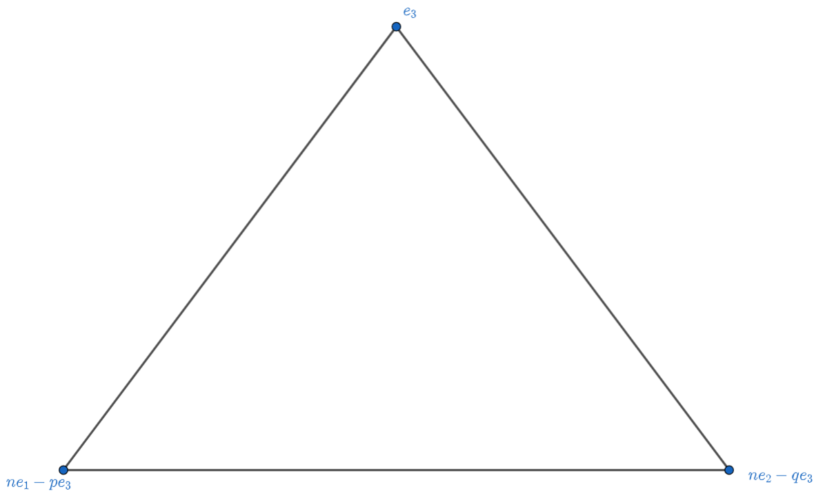
Figure 3. Transversal section of $\sigma$.

The fan defined by the cone $\sigma$ has 2-dimensional faces (walls) given by $\tau_{jk}=C(d_{j},d_{k})$ for $j<k$. By Section 7.1, each wall $\tau_{jk}$ can be resolved by Hirzebruch-Jung sequences $(m_{jk,\alpha},n_{jk,\alpha})_{\alpha=0}^{s_{jk}+1}$ in direction $d_{j}$ to $d_{k}$ with initial data

$$m_{jk,0}=n,\quad n_{jk,0}=0,\quad n_{jk,1}=1,\quad\forall j<k,$$

$$m_{13,1}=p^{\prime},\quad m_{23,1}=q^{\prime},\quad m_{12,1}=\{-p^{\prime}q\}_{n},$$

where $p^{\prime}$ and $q^{\prime}$ are the inverse modulo $n$ of $p$ and $q$. Thus, there are integers $k_{jk,\alpha}\geq 2$, such that

$$\frac{n}{m_{jk,1}}=[k_{jk,1},...,k_{jk,s_{jk}}].$$

Then, the walls $\tau_{jk}$ can be resolved by subdividing them in a sequence of steps by rays with generators $(e_{jk,\alpha})_{\alpha=1}^{s_{jk}}$ defined recursively as

$$e_{jk,\alpha}=\frac{m_{jk,\alpha}d_{j}+n_{jk,\alpha}d_{k}}{n},\quad 1\leq\alpha\leq s_{jk}.$$

If we fix $j<k$, we denote by $e_{kj,\alpha}$ the exceptional divisors in direction $d_{k}$ to $d_{j}$. We have the relation $e_{jk,\alpha}=e_{kj,s+1-\alpha}$. In Figure 4 are illustrated the border generators.

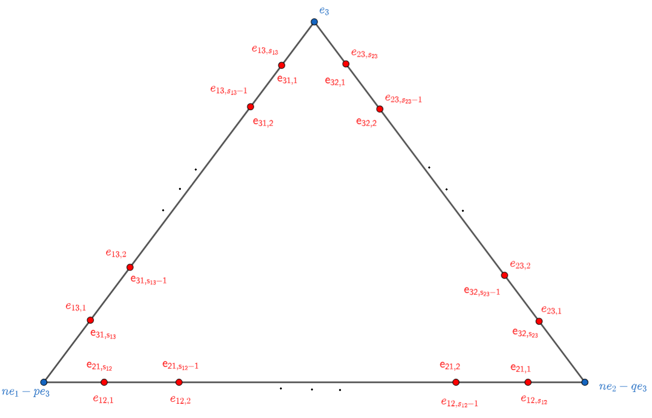
Figure 4. Lattice points that resolve each wall

In order to choose a good asymptotic local resolution of $\sigma$, imitating the $2$-dimensional case, we can ask for a minimal local resolution, i.e., with nef canonical bundles. However, minimal varieties in higher dimensions may have terminal singularities, minimal singular models are not necessarily unique, and there are no efficient algorithms in the toric case. In this last, at least there exists a kind of optimal method. Minimal resolutions can be obtained by the canonical resolution of $\sigma$ which is obtained by the canonical refinement of the cone [CLS11, Prop. 11.4.15]. However, the canonical refinement appears not to have a regular pattern for any $p,q$. For example, if $p=n-1$, and $0<q<n$ are free, the canonical and minimal resolutions look very simple but release a lot of exceptional data. See Figure 5. The resolution to the case $p=q$ takes the same form, just rotate the figure. And completely different from the above is the case $p+q=n$. See Figure 6. Thus, we do not consider these cases in the following, i.e., $p,q\neq n-1$, $p=q$ or $\{p+q\}_{n}=0$.

Figure 5. Case $p=n-1$. We have cones generated by 4 generators. These cones define the canonical resolution of $\sigma$. The black dots, mark lattice points to blowing up and get a minimal non-singular resolution.

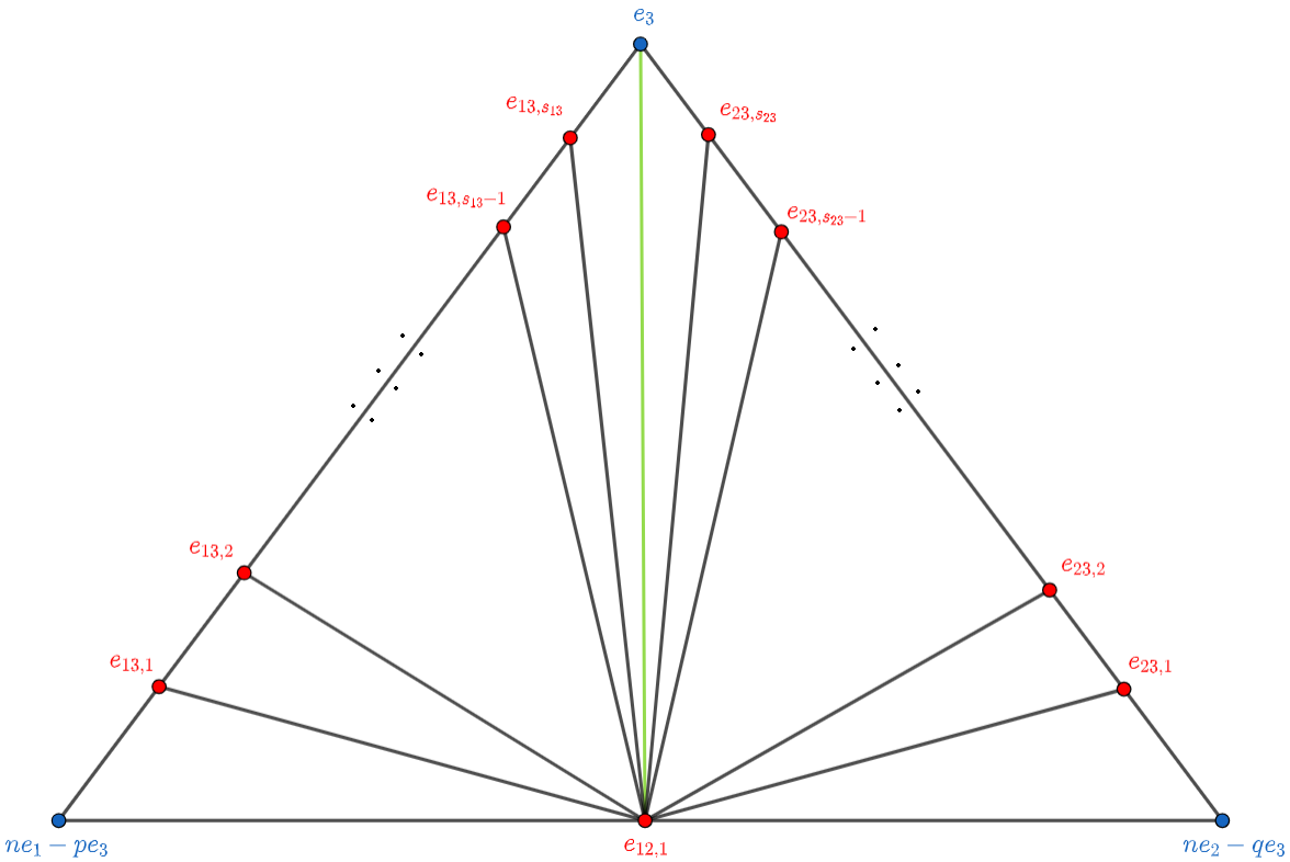
Figure 6. Case $p+q=n$. The wall $\tau_{12}$ is of type $(1,1)/n$. Then the minimal non-singular resolution depends only on the resolutions of the other walls.

In order to have a systematic way to construct resolutions, we choose the following way: We construct a cyclic resolution, i.e., a refinement of $\sigma$ composed by $3$-cones defining cyclic singularities. The advantage of this resolution is that the local canonical bundle is almost nef, i.e., there are no more than $3$ negative curves. As an optional step, we can use the Fujiki-Oka algorithm to resolve these cyclic singularities. Under some conditions, these resolutions have good asymptotical behavior with respect to $n$.

4.2.1. Cyclic resolution.

From (4) we know that every $v\in P_{\sigma}\cap N$ can be written as

$$v=\frac{v_{1}d_{1}+v_{2}d_{2}+v_{3}d_{3}}{n},\quad v_{3}=\{pv_{1}+qv_{2}\}_{n}\quad 0\leq v_{i}<n.$$

Fix a $v$, with $v_{1}+v_{2}+v_{3}\leq n$ and $v_{i}>0$.

Step 1: We refine by a star subdivision along $v$ obtaining a fan as illustrate Figure 7.

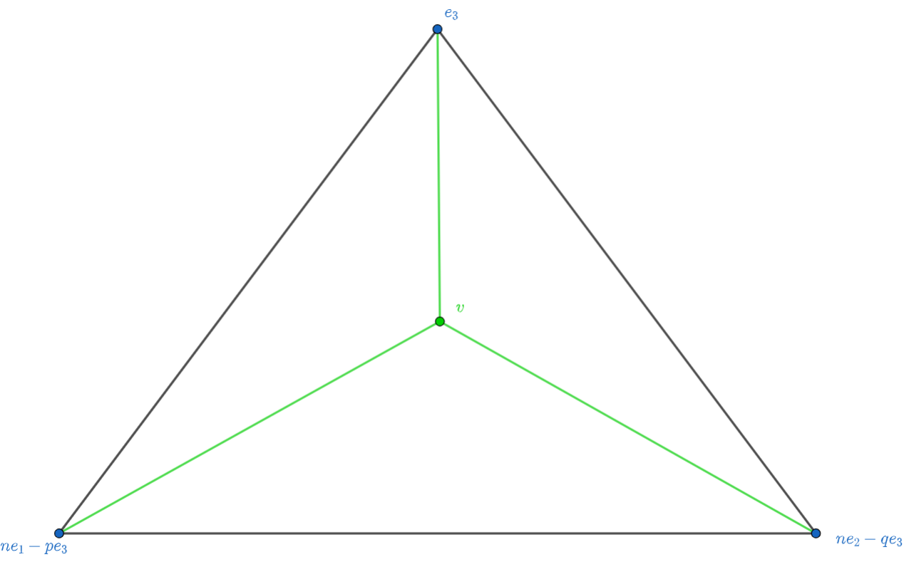
Figure 7. Star subdivision along minimizer $v$

Step 2: Now we refine each wall by doing toric blow-ups following the Hirzebruch-Jung algorithm. So we obtain a refinement $\sigma^{*}$ and denote by $X$ the toric variety associated. This refinement gives us a birational projective morphism $g\colon X\to Y_{p,q}$ [CLS11, 11.1.6]. This refinement is sketched in Figure 8.

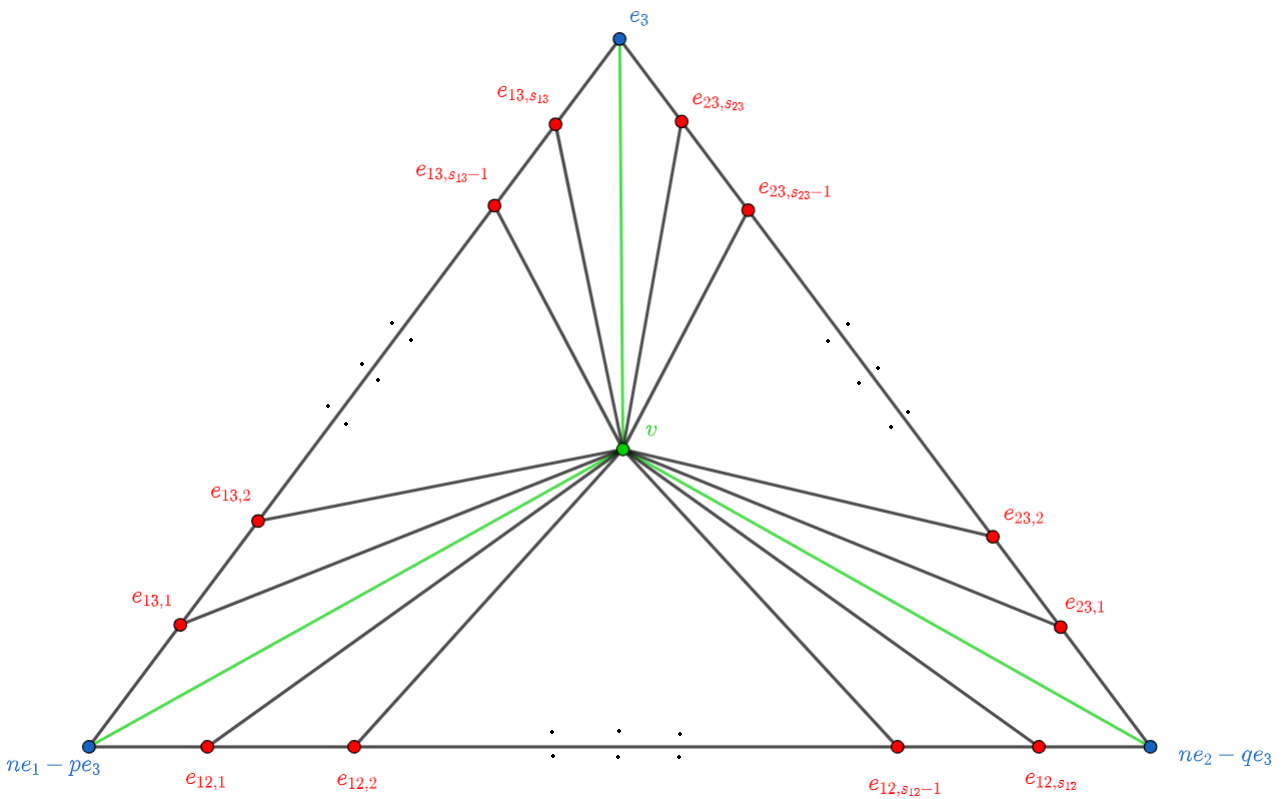
Figure 8. Cyclic local resolution

Denote each $3$-cone of $\sigma^{*}$ by

$$\sigma_{jk,\alpha}=C(v,e_{jk,\alpha},e_{jk,\alpha+1}),\quad 0\leq\alpha\leq s_{jk}.$$

The $2$-cones of $\sigma^{*}$ are given in two types. The exterior walls $\tau_{jk,\alpha}=C(e_{jk,\alpha},e_{jk,\alpha+1})$, and the inner walls $\rho_{jk,\alpha}=C(v,e_{jk,\alpha})$. For any permutation $(v_{j},v_{k},v_{l})$ with $j<k$, using determinants and properties of Section 7.1, we have

$$\mbox{mult}(\sigma_{jk,\alpha})=v_{l},\quad\mbox{mult}(\rho_{jk,\alpha})=\mbox{gcd}(v_{j}n_{jk,\alpha}-v_{k}m_{jk,\alpha},v_{l}),\quad\mbox{mult}(\tau_{jk,\alpha})=1.$$

Lemma 4.3.

Each cone $\sigma_{jk,\alpha}$ is a cyclic singularity of type

$$\frac{(a_{jk,\alpha},b_{jk,\alpha},1)}{v_{l}},\quad a_{jk,\alpha}=\{m_{jk,\alpha+1}v_{k}-n_{jk,\alpha+1}v_{j}\}_{v_{l}},\quad b_{jk,\alpha}=\{m_{jk,\alpha}v_{k}-n_{jk,\alpha}v_{j}\}_{v_{l}},$$

where $\{\cdot\}_{v_{l}}$ is the residue modulo $v_{l}$.

Proof.

Since $\tau_{jk,\alpha}$ is non-singular, then $\sigma_{jk,\alpha}$ is semi-unimodular respect to $v$. By [Ash15, Prop. 1.2.3] if there is positive integer $x,y$ such that

$$\frac{xe_{jk,\alpha}+ye_{jk,\alpha+1}+v}{v_{l}}\in{\mathbb{Z}}^{3},$$

then $x,y$ define the type of the cyclic singularity. Since $\gcd(n,v_{l})=1$, we can solve the equations modulo $v_{l}$ and the result follows.
∎

Denote by $h\colon X\to Y_{p,q}\to{\mathbb{A}}^{3}$ the composition with the natural projection to ${\mathbb{A}}^{3}$. Denote by $D_{j}$ the divisor in ${\mathbb{A}}^{3}$ defined by the coordinate $x_{j}$. Each ray on $\sigma^{*}$ generated by $d_{j},e_{jk,\alpha},$ or $v$ defines a toric divisor on $X$ given by

$$\tilde{D}_{j}=V(C(d_{j})),\quad E_{jk,\alpha}=V(C(e_{jk,\alpha})),\quad F=V(C(v)),$$

where $V(\cdot)$ denotes the orbit closure of a cone [CLS11, p. 121]. At the same time we fix notation for $j<k$ by $E_{kj,\alpha}:=E_{jk,s+1-\alpha}$. we can compute

$$h^{*}D_{j}=n\tilde{D}_{j}+\sum_{k}\sum_{\alpha=1}^{s_{jk}}m_{jk,\alpha}E_{jk,\alpha}+v_{j}F,$$

$$K_{X}=g^{*}K_{Y_{p,q}}+\sum_{j<k}\sum_{\alpha=1}^{s_{jk}}N_{jk,\alpha}E_{jk,\alpha}+\frac{v_{1}+v_{2}+v_{3}-n}{n}F,$$ (5)

where

$$N_{jk,\alpha}:=\frac{m_{jk,\alpha}+n_{jk,\alpha}}{n}-1.$$

It is satisfied the relation $k_{jk,\alpha}N_{jk,\alpha}-N_{jk,\alpha+1}=N_{jk,\alpha-1}-(k_{jk,\alpha}-2),$ which gives

$$\sum_{\alpha=1}^{s_{jk}}N_{jk,\alpha}(k_{jk,\alpha}-2)=-(N_{jk,1}+N_{kj,1})-\sum_{\alpha=1}^{s_{jk}}(k_{jk,\alpha}-2).$$

Proposition 4.4.

The ${\mathbb{Q}}$-divisor

$$h^{*}\left(\frac{n-1}{n}(D_{1}+D_{2}+D_{3})\right)+\sum_{j<k}\sum_{\alpha}N_{jk,\alpha}E_{jk,\alpha}+\frac{v_{1}+v_{2}+v_{3}-n}{n}F,$$

is an effective ${\mathbb{Z}}$-divisor.

Proof.

The local pullback $h^{*}(D_{1}+D_{2}+D_{3})$ equals

$$n(\tilde{D_{1}}+\tilde{D_{2}}+\tilde{D_{3}})+\sum_{j<k,\alpha}(m_{jk,\alpha}+n_{jk,\alpha})E_{jk,\alpha}+(v_{1}+v_{2}+v_{3})F_{jkl,p}.$$

Thus, $h^{*}\left(\frac{n-1}{n}(D_{j}+D_{k}+D_{l})\right)+\Delta$ equals to

$$(n-1)(\tilde{D_{1}}+\tilde{D_{2}}+\tilde{D_{3}})+\sum_{j<k,\alpha}\left(m_{jk,\alpha}+n_{jk,\alpha}-1\right)E_{jk,\alpha}+(v_{1}+v_{2}+v_{3}-1)F,$$

i.e., an effective ${\mathbb{Z}}$-divisor. ∎

Each inner wall defines a closed curve on $X$ given by

$$C_{j}=V(C(d_{j},v)),\quad C_{jk,\alpha}=V(C(\rho_{jk,\alpha})).$$

The refinement $\sigma^{*}$ is simplicial with cones of multiplicity one, and the canonical divisor $K_{X}$ is a ${\mathbb{Q}}$-Cartier divisor. For any pair $v_{j},v_{k}$, $j<k$, let $v_{l}$ be the another coordinate. The following relation among lattices generators,

$$e_{jk,\alpha-1}+(-k_{jk,\alpha})e_{jk,\alpha}+0\cdot v+e_{jk,\alpha+1}=0,$$

$$v_{j}e_{lj,1}+\left(\frac{v_{l}-m_{lj,1}v_{j}-m_{lk,1}v_{k}}{n}\right)d_{l}+(-1)v+v_{k}e_{lk,1}=0,$$

describe the intersection theory on $X$ [Ful93, Ch. V]. We have,

$$E_{jk,\alpha}C_{jk,\alpha\pm 1}=\frac{\mbox{mult}(\rho_{jk,\alpha})}{v_{l}},\quad E_{jk,\alpha}C_{jk,\alpha}=-\frac{k_{jk,\alpha}\mbox{mult}(\rho_{jk,\alpha})}{v_{l}},\quad FC_{jk,\alpha}=0,$$

$$\tilde{D}_{l}\,C_{l}=\frac{\gcd(v_{j},v_{k})(v_{l}-m_{lj,1}v_{j}-m_{lk,1}v_{k}))}{nv_{j}v_{k}},\quad F\,C_{l}=-\frac{\gcd(v_{j},v_{k})}{v_{j}v_{k}},$$

$$K_{X}\,C_{l}=-\frac{\gcd(v_{j},v_{k})}{v_{j}v_{k}}\left(v_{j}+v_{k}-1+\frac{v_{l}-m_{lj,1}v_{j}-m_{lk,1}v_{k}}{n}\right),$$

$$K_{X}\,C_{jk,\alpha}=\frac{\mbox{mult}(\rho_{jk,\alpha})}{v_{l}}(k_{jk,\alpha}-2),\quad 1\leq\alpha\leq s_{jk}.$$ (6)

Lemma 4.5.

We have

$$F^{3}=\frac{n}{v_{1}v_{2}v_{3}}.$$

Proof.

The divisor $v_{j}F$ is Cartier for any $j$, then from the pullback identities above we have

$$v_{1}v_{2}v_{3}F^{3}=\prod_{j=1}^{3}\left(h^{*}D_{j}-nD_{j}-\sum_{k}\sum_{\alpha}m_{jk,\alpha}E_{jk,\alpha}\right)=h^{*}D_{1}\,h^{*}D_{2}\,h^{*}D_{3}=n,$$

where the last is by projection formula.∎

As a consequence, we can compute,

$$K_{X}F^{2} =-F^{2}\left(D_{1}+D_{2}+D_{3}+F\right)$$

$$=\frac{v_{1}+v_{2}+v_{3}-n}{v_{1}v_{2}v_{3}}.$$

From the last one, we get

$$K_{X}^{2}\,F =-\sum_{l}\frac{K_{X}\,C_{l}}{\gcd(v_{j},v_{k})}-\sum_{j<k,\alpha}\frac{K_{X}\,C_{jk,\alpha}}{\mbox{mult}(\rho_{jk,\alpha})}-K_{X}F^{2}.$$

The following arithmetic lemma will be useful in Section 4.3.

Lemma 4.6.

There exists $v\in P_{\sigma}\cap N$ such that $v_{1}+v_{2}+v_{3}=n$, so $K_{X}$ has multiplicity zero at $F$. Moreover, for $n\gg 0$ we can choose $v$ such that the slopes $v_{j}/v_{k}\leq 3$.

Proof.

By (4) we have $v_{3}=\{v_{1}p+v_{2}q\}_{n}$. So $v_{1}+v_{2}+v_{3}=n$, implies that $(v_{1},v_{2})$ are solutions $(x,y)$ of the Diophantine equation

$$y\equiv cx\mod n,\quad c=\{-(p+1)(q+1)^{\prime}\}_{n}.$$

Moreover, for any of those solutions with $x+y<n$, we have $v_{3}=n-x-y$. A degenerate case is $p+q=n-2$, equivalently $c=1$, thus the solution to the equation is the diagonal. Thus, we can choose $x=y=\lfloor\frac{n}{3}\rfloor$, and the result follows for this case. Now, we assume that $c<n/2$, otherwise we do $(x,y)\mapsto(-x,y)$. The integer points in the square $[1,n-1]^{2}$ solving the equation distribute in ${\mathbb{R}}^{2}$ along the lines $L_{\beta}:y=cx-\beta n$ for $0\leq\beta\leq c-1$. Thus, over each $L_{\beta}$ the integer solutions over the line are defined by those integers in the interval

$$I_{\beta}=\left(\left\lfloor\frac{\beta n}{c}\right\rfloor,\left\lfloor\frac{(\beta+1)n}{c}\right\rfloor\right].$$

For each $1\leq k\leq\lfloor\frac{n}{c}\rfloor$, we have

$$y_{k}=y\left(\left\lfloor\frac{\beta n}{c}\right\rfloor+k\right)=ck-r,$$

where $0\leq r<c$ is the residue of $\beta n$ modulo $c$. So, $c(k-1)\leq y_{k}\leq ck$. Let us choose $\beta=\lfloor\frac{c-1}{3}\rfloor,$ and $k=\lfloor\frac{n}{3c}\rfloor$. In particular $\lfloor\frac{n}{3}\rfloor\in I_{\beta}$. So, as $n\gg 0$ we have $y_{k}\approx\frac{n}{3}$. By construction, we have $x_{k}=\left\lfloor\frac{\beta n}{c}\right\rfloor+k$. Let $0\leq r^{*}\leq 2$ the residue of $c-1$ modulo $3$, then $x_{k}\approx\frac{n(c-r^{*})}{3c}$. Since $\frac{1}{2}\leq\frac{c-r^{*}}{c}\leq 1$, the result follows choosing $v_{1}=x_{k}$ and $v_{2}=y_{k}$ as $n\gg 0$. ∎

Example 4.7.

Case $\{p+q\}_{n}=1$: For $v_{1}=v_{2}=1$, we have $v_{3}=\{p+q\}_{n}=1$. Thus, these coordinates define an interior lattice point $v$, and it minimizes $v_{1}+v_{2}+v_{3}$. We have

$$\mbox{mult}(\sigma_{jk,\alpha})=\mbox{mult}(\rho_{jk,\alpha})=\mbox{mult}(\tau_{jk,\alpha})=1,$$

i.e., $X$ is non-singular. On the other hand,

$$K_{X}C_{jk,\alpha}=(k_{jk,\alpha}-2),\quad K_{X}C_{l}=0,$$

for all $j,k$ and $l$. Thus, $K_{X}$ is nef.

Example 4.8.

Case $\{p+q\}_{n}=2$: In this case, again $v_{1}=v_{2}=1$ defines the minimizer interior lattice point $v$. In this case, we have $\sigma_{13,\alpha}$ and $\sigma_{23,\alpha}$ as non-singular cones. On the other hand, each $\sigma_{12,\alpha}$ is cyclic singularity of order $2$. Thus, they define canonical and terminal singularities. The first ones achieve a terminal resolution with one blow-up. Moreover,

$$K_{X}C_{3}=0,\quad K_{X}C_{j}\in\left\{0,-\frac{1}{2}\right\},\quad j=1,2$$

so there are $p,q$ with canonical divisor $K_{X}$ nef. In the worst case, i.e., $K_{X}\,C_{j}<0$ for $j=1,2$, we can do toric flips a to get a nef toric variety given whose fan is sketched in Figure 9.

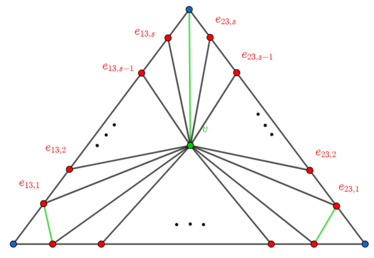
Figure 9. Flipped fan for $\{p+q\}_{n}=2$.

Example 4.9.

If we drag the lattice point $v$ to one of the generators of the cone $\sigma$, we get a degenerated fan as in Figure 10. In this case, the singularities are of order $n$, and as an advantage, we do not have a divisor $F$.

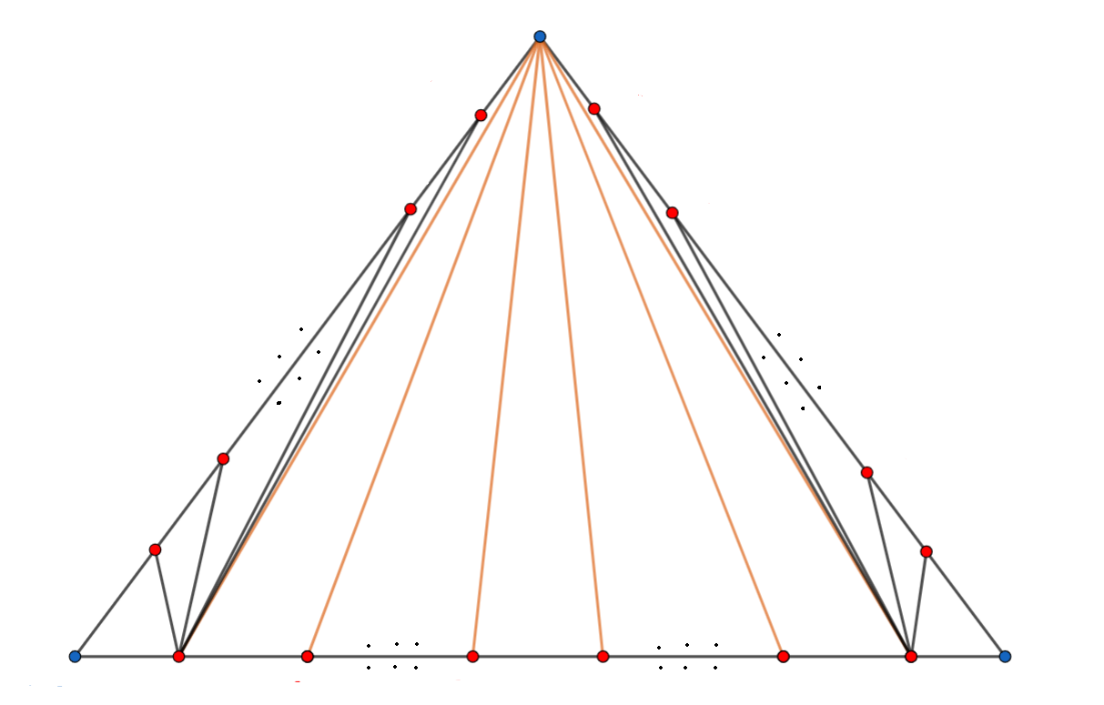
Figure 10. Degenerated cyclic resolution

As we see, having $v_{j}\leq 2$ gives us good singularities to work. Indeed, if the $v_{j}^{\prime}s$ are small enough, the singularities are also good in asymptotic terms.

Step 3 (Optional): Now we can desingularize each non-terminal cyclic singularity using the Fujiki-Oka algorithm. See [Ash19] for a modern treatment. Denote the complete resolution as $\tilde{X}\to X\to Y_{p,q}$. Since the cone of toric cyclic singularities of any type $\frac{a,b}{c}$ has multiplicity $c$, then there is a resolution of singularities with length at most $c$. In this case, if we assume $v_{j}$ bounded by $n^{1/C}$ with $C\geq 1$, then the lengths on $\sigma^{*}$ can be bounded by

$$\sum_{j<k}s_{jk}n^{1/C}\leq 3C^{\prime}n^{2/C},$$

for another constant $C^{\prime}>0$ using the result of Girstmair (Theorem 2.26). For $C>2$, it is guaranteed that $\tilde{X}$ is a resolution of singularities with good asymptotical behavior.

4.3. Global resolution

Let $\{D_{1},...,D_{r}\}$ be an asymptotic arrangement on $Z$. Thus, for prime numbers $n\gg 0$ we have multiplicities $0<\nu_{j}<n$ depending on $n$, with its respective $q_{jk}\in O_{n}$. We have $n$-th root covers $f_{n}\colon Y_{n}\to Z$ branched at each $D=\sum_{j}\nu_{j}D_{j}$. Let us fix a $n\gg 0$, so we drop the subscript $n$ of the morphisms, i.e., we are fixing a $f\colon Y_{n}\to Z$.

For $j<k$, the singularities of $Y_{n}$ over curves in $D_{jk}:=D_{j}\cap D_{k}$ are locally analytically isomorphic to $C_{q_{jk},n}\times{\mathbb{C}}$ where $C_{q_{jk},n}$ is the surface cyclic quotient singularity of type $\frac{1}{n}(q_{jk},1)$. For a triple $j<k<l$, the singularity of $Y_{n}$ over a point in $D_{jkl}:=D_{j}\cap D_{k}\cap D_{l}$ is locally analytically isomorphic to the normalization of $\mbox{Spec}(\sigma_{jkl}^{\vee}\cap M)$ where $\sigma_{jkl}$ is a cone with walls of types $\frac{1}{n}(q_{jk},1),\frac{1}{n}(q_{jl},1),\frac{1}{n}(q_{kl},1)$ as we see in Section 4.2. We will get the cyclic resolution $X_{n}\to Y_{n}$ via weighted blow-ups in two steps.

Step 1: Since singularities over $D_{jkl}$ are isolated, for each $\sigma_{jkl}$, we do a weighted blow-up at a convenient interior lattice point $v^{jkl}$. So, this refinement locally gives a projective morphism which is a blow-up over an isolated point [CLS11, 11.1.6]. In this case, we get a projective birational morphism $h^{\prime}:X_{n}^{\prime}\to Y_{n}$. We have exceptional divisors $F_{jkl}$ whose components are over the points of $D_{jkl}$ and they are isomorphic to weighted fake projective planes [Buc08]. For future computations, we fix the notation of $v^{jkl}$ and $F_{jkl}$ independent of the order of the triple $j,k,l$. For example, $v^{jkl}=v^{kjl}$.

Step 2: Since the centers of the above blow-ups are points, the singularity type over intersections $D_{jk}$ was not affected. For curves in $D_{jk}$, locally by SNC property, we can assume that they are supported on a local equation $xy=0$ for local coordinates $x,y$. Then over such curves, the singularities on $X^{\prime}_{n}$ are locally analytically isomorphic to $C_{q_{jk},n}\times{\mathbb{C}}$, thus we use the Hirzebruch-Jung algorithm which is a weighted blow-up to resolve $C_{q_{jk},n}$. The Hirzebruch-Jung resolution can be realized by a single blow-up $Bl_{{\mathfrak{m}}}(C_{q_{jk,n}})\to C_{q_{jk,}}$ where ${\mathfrak{m}}$ is a maximal ideal determined explicitly in coordinates $x,y$ as we see at the end of Section 7.1 (also see [KM92, 10.5]). In terms of local resolutions, we need to follow an order compatible with the resolution, i.e., if we locally blow-up a curve in $D_{jk}$ then this operation must be reflected on the other local toric pictures following the centers to blowing-up. See Figure 11. Thus, this construction extends and we have resolved the curves $D_{jk}$. Consequently, we get a projective morphism denoted by $g\colon X_{n}\to X^{\prime}_{n}\to Y_{n}$, and denote by $h\colon X_{n}\to Z$ the composition. Since $X_{n}$ was constructed by a sequence of weighted blow-ups with cyclic singularities, then, $X_{n}$ is an embedded ${\mathbb{Q}}$-resolution of $Y_{n}$ [ABMMOG12, 2.1]. As we see in 2.21, the varieties $X_{n}$ are irreducible. We summarize this in the following.

Proposition 4.10 (and Definition).

There exists a cyclic partial resolution $g:X_{n}\to Y_{n}$, i.e. a projective, surjective, birational morphism such that $X_{n}$ is irreducible and, it has at most isolated cyclic quotient singularities of order lower than $n$.

∎

Figure 11. Assume $r=4$ with $D_{jkl}=1$, then on $Y$ the singularities over each $D_{jkl}$ can be sketched as in the figure. So the resolution process is in the following order: First the internals blow-ups, and then the walls in the following order $D_{12},D_{13},D_{14},D_{23},D_{24},D_{34}$.

In the rest, we will abuse notation using $D_{jk}$ and $D_{jkl}$ for both, set-theoretic intersections $D_{j}\cap D_{k}$ and $D_{j}\cap D_{k}\cap D_{l}$, and for intersections of cycles $D_{j}D_{k}$ and $D_{j}D_{k}D_{l}$. Over each $D_{jk}$, we get exceptional divisors $E_{jk,\alpha}$, $0\leq\alpha\leq s_{jk}$, where $s_{jk}=\ell(n,q_{jk})$ and whose components are over those of $D_{jk}$. From the local computations of the section above, we have

$$h^{*}D_{j}=n\tilde{D}_{j}+\sum_{D_{k}D_{j}\neq\emptyset}\sum_{\alpha=1}^{s_{jk}}m_{jk,\alpha}E_{jk,\alpha}+\sum_{D_{kl}D_{j}\neq\emptyset}{F_{kl,j}},$$ (7)

where $F_{kl,j}$ is a divisor whose components are the exceptional divisors over points in $D_{jkl}$.

Explicitly, for any triple of positive integers numbers $j,k,l$, let $\rho_{kl}(j)\in\{1,2,3\}$ the position of $j$ if we order the triple. For example $\rho_{23}(1)=1$, $\rho_{57}(6)=2$ or $\rho_{54}(8)=3$. Thus, if $F_{jkl,p}$ is the exceptional divisor over a point $p\in D_{jkl}$, then

$$F_{jkl}=\sum_{p\in D_{jkl}}F_{jkl,p}$$

$$F_{kl,j}=\sum_{p\in D_{jkl}}\rho_{kl}(j)F_{jkl,p}.$$ (8)

In terms of intersection theory, we have

$$F_{jkl}^{3}=\frac{n}{v^{jkl}_{1}v^{jkl}_{2}v^{jkl}_{3}}D_{jkl},\quad\tilde{D_{j}}\tilde{D_{k}}=0.$$

From Theorem 2.18 we have $K_{X_{n}}\sim_{{\mathbb{Q}}}h^{*}(K_{Z}+\frac{n-1}{n}\sum_{j}D_{j})+\Delta$ where

$$\Delta=\sum_{j<k}E_{jk}+\sum_{j<k<l}V_{jkl}F_{jkl},$$

$$V_{jkl}=\frac{v_{1}^{jkl}+v_{2}^{jkl}+v_{3}^{jkl}-n}{n},$$

$$E_{jk}=\sum_{\alpha=1}^{s_{jk}}N_{jk,\alpha}E_{jk,\alpha}.$$

The following proposition will be useful in Section 5. First recall that on a variety $X$ a curve $C$ is $K_{X}$-negative, $K_{X}$-positive or $K_{X}$-trivial if its intersection with the canonical divisor is negative, positive, or zero.

Proposition 4.11.

The ${\mathbb{Q}}$-divisor $h^{*}\left(\frac{n-1}{n}\sum_{i=1}^{r}D_{i}\right)+\Delta$ is an effective ${\mathbb{Z}}$-divisor. Thus, if $K_{Z}$ is nef, then the $K_{X_{n}}$-negative curves of $X_{n}$ are contained in the support of $h^{*}D$.

Proof.

The first assertion is a direct consequence of 4.4. Now assume that $K_{Z}$ is nef, and let $C$ be a curve in $X$. If $C$ is not contained in the support of $h^{*}D$, then

$$K_{X_{n}}\,C=\left(h^{*}\left(K_{Z}+\frac{n-1}{n}\sum_{i=1}^{r}D_{i}\right)+\Delta\right).C>0,$$

since $h^{*}K_{Z}$ is nef (projection formula), and effectiveness of $h^{*}\left(\frac{n-1}{n}\sum_{i=1}^{r}D_{i}\right)+\Delta$. Thus, if $C$ is negative must lie in the support of $h^{*}D$.
∎

Now we describe how the intersection theory on $X_{n}$ behaves under pullbacks of divisors of $Z$. In what follows, we set $E_{jk,0}=\tilde{D}_{j}$ and $E_{jk,s_{jk}+1}=\tilde{D}_{k}$.

Proposition 4.12.

Let $G,G^{\prime}$ any divisors on $Z$, then $h^{*}GF_{kl,j}=0$ as $2$-cycle, for any $1\leq\alpha\leq s_{jk}$,

$$h^{*}Gh^{*}G^{\prime}E_{jk,\alpha}=0,$$

$$h^{*}GE_{jk,\alpha}^{2}=-k_{jk,\alpha}GD_{jk},\quad h^{*}GE_{jk,\alpha}E_{jk,\alpha\pm 1}=GD_{jk}.$$

Proof.

We use the projection formula repeatedly. The first one is given by the fact that $h_{*}F_{jk,l}$ has codimension $3$. Now for a $1\leq\alpha\leq s_{jk}$ we have $h_{*}E_{jk,\alpha}$ supported in codimension $2$, thus

$$h^{*}Gh^{*}G^{\prime}E_{jk,\alpha}=GG^{\prime}h_{*}E_{jk,\alpha}=0.$$

Finally, for any $\alpha$ we have

$$h^{*}D_{j}h^{*}GE_{jk,\alpha}=0=h^{*}G(m_{jk,\alpha-1}E_{jk,\alpha-1}E_{jk,\alpha}+m_{jk,\alpha}E_{jk,\alpha}^{2}+m_{jk,\alpha+1}E_{jk,\alpha+1}E_{jk,\alpha}),$$

$$h^{*}D_{k}h^{*}GE_{jk,\alpha}=0=h^{*}G(n_{jk,\alpha-1}E_{jk,\alpha-1}E_{jk,\alpha}+n_{jk,\alpha}E_{jk,\alpha}^{2}+n_{jk,\alpha+1}E_{jk,\alpha+1}E_{jk,\alpha}).$$

The recursive relations with $k_{jk,\alpha}$ give

$$\left[\begin{array}[]{cc}m_{jk,\alpha}&m_{jk,\alpha+1}\\ n_{jk,\alpha}&n_{jk,\alpha+1}\\ \end{array}\right]\left[\begin{array}[]{c}h^{*}G(E_{jk,\alpha}^{2}+k_{jk,\alpha}E_{jk,\alpha-1}E_{jk,\alpha})\\ h^{*}G(E_{jk,\alpha+1}E_{jk,\alpha}-E_{jk,\alpha-1}E_{jk,\alpha})\end{array}\right]=\left[\begin{array}[]{c}0\\ 0\end{array}\right].$$

From Lemma 7.2 we have the determinant $m_{jk,\alpha}n_{jk\alpha+1}-m_{jk,\alpha+1}n_{jk,\alpha}=n$, thus

$$h^{*}G(E_{jk,\alpha}^{2}+k_{jk,\alpha}E_{jk,\alpha-1}E_{jk,\alpha})=0$$

$$h^{*}G(E_{jk,\alpha+1}E_{jk,\alpha}-E_{jk,\alpha-1}E_{jk,\alpha})=0.$$

In particular, we have

$$h^{*}GE_{jk,\alpha+1}E_{jk,\alpha}=h^{*}G\tilde{D}_{j}E_{jk,1}=GD_{jk},$$

and the result follows. ∎

Corollary 4.13.

For any divisor $G$ on $Z$ we have

$$h^{*}GE_{jk}K_{X}=-D_{jk}G\left((N_{jk,1}+N_{kj,1})+\sum_{\alpha=1}^{s_{jk}}(k_{jk,\alpha}-2)\right).$$

Proof.

Since $h^{*}G\,F$ vanishes at top-dimensional intersections, and $E_{jk,\alpha_{1}}E_{jk,\alpha_{2}}=0$ for $|\alpha_{1}-\alpha_{2}|>1$, we have

$$h^{*}GE_{jk}K_{X} =h^{*}G(E_{jk})^{2}=h^{*}G\sum_{\alpha=1}^{s_{jk}}N_{jk,\alpha}^{2}E_{jk,\alpha}^{2}+2N_{jk,\alpha}N_{jk,\alpha+1}E_{jk,\alpha}E_{jk,\alpha+1}$$

$$=D_{jk}G\sum_{\alpha=1}^{s_{jk}}-k_{jk,\alpha}N_{jk,\alpha}^{2}+2N_{jk,\alpha}N_{jk,\alpha+1}$$

$$=D_{jk}G\sum_{\alpha=1}^{s_{jk}}N_{jk,\alpha}N_{jk,\alpha+1}-N_{jk,\alpha}N_{jk,\alpha-1}+N_{jk,\alpha}(k_{jk,\alpha}-2)$$

$$=D_{jk}G\sum_{\alpha=1}^{s_{jk}}N_{jk,\alpha}(k_{jk,\alpha}-2)$$

$$=-D_{jk}G\left((N_{jk,1}+N_{kj,1})+\sum_{\alpha=1}^{s_{jk}}(k_{jk,\alpha}-2)\right).$$

where the last identity is by telescoping sum argument. ∎

Corollary 4.14.

If $C$ is a curve on $X_{n}$ contained in $\tilde{H}_{j}$ and disjoint to any exceptional divisor $F_{jkl}$, then

$$\tilde{D}_{j}C=\frac{h_{*}C}{n}\left(D_{j}-\sum_{j\neq k}m_{jk,1}D_{k}\right).$$

Proof.

From (7) we have

$$h^{*}D_{j}C=D_{j}h_{*}C=n\tilde{D}_{j}+\sum_{k}m_{jk,1}E_{jk,1}C,$$

$$h^{*}D_{k}C=D_{k}h_{*}C=E_{jk,1}C,\quad\forall j\neq k,$$

and the result follows. ∎

4.3.1. Asymptoticity of $K_{X_{n}}^{3}$.

For simplicity, let us denote $K_{X}=K_{X_{n}}$. Let us introduce the following notation

$$|D|_{jk}:=|D_{j}|_{k}+|D_{k}|_{j},$$

where $|D_{j}|_{k}$ satisfy

$$\sum_{D_{ll^{\prime}}D_{j}\neq 0}F_{ll^{\prime},j}E_{jk,\alpha}K_{X}=|D_{j}|_{k}(k_{jk,\alpha}-2).$$

Remark 4.15.

Using equations from (6), observe that $|D_{j}|_{k}$ depends on slopes of weights $v^{jkl}_{1},v^{jkl}_{2},v^{jkl}_{3}$ of the lattice points $v^{jkl}$. Explicitly, using (8), we have

$$|D_{j}|_{k}=\sum_{l}\dfrac{v^{jkl}_{\rho_{kl}(j)}}{{v^{jkl}_{\rho_{kj}(l)}}}D_{jkl}.$$

We need this to compute the intersection of $K_{X}$ with the external walls of the local toric resolution. Recursively we denote,

$$x_{jk,\alpha}=K_{X}E_{jk,\alpha-1}E_{jk,\alpha},\quad 1\leq\alpha\leq s_{jk}+1$$

$$y_{jk,\alpha}=K_{X}E_{jk,\alpha}^{2},\quad 1\leq\alpha\leq s_{jk}.$$

Thus, we can write

$$h^{*}D_{j}E_{jk,\alpha}K_{X}=m_{jk,\alpha-1}x_{jk,\alpha}+m_{jk,\alpha}y_{jk,\alpha}+m_{jk,\alpha+1}x_{jk,\alpha+1}+|D_{j}|_{k}(k_{jk,\alpha}-2)$$ (9)

Using the ${\mathbb{Q}}$-numerical equivalence of $K_{X}$ in 2.18, we compute

$$x_{jk,1}=h^{*}D_{k}\tilde{D_{j}}K_{X}=D_{jk}\left(K+\sum_{l\neq j}N_{jl,1}D_{l}\right),$$

$$x_{jk,s+1}=h^{*}D_{j}\tilde{D_{k}}K_{X}=D_{jk}\left(K+\sum_{l\neq k}N_{kl,1}D_{l}\right).$$

Proposition 4.16.

We have

$$x_{jk,\alpha}=x_{jk,1}+\frac{1}{n}(m_{jk,\alpha}^{*}(D_{jk}D_{k}-|D_{k}|_{j})-n_{jk,\alpha}^{*}(D_{jk}D_{j}-|D_{j}|_{k})),$$

$$y_{jk,\alpha}=-k_{jk,\alpha}x_{jk,\alpha}+\frac{(k_{jk,\alpha}-2)}{n}(n_{jk,\alpha+1}(D_{jk}D_{j}-|D_{j}|_{k})-m_{jk,\alpha+1}(D_{jk}D_{k}-|D_{k}|_{j})).$$

Where $m_{jk,\alpha}^{*}=m_{jk,\alpha}-m_{jk,\alpha-1}-m_{jk,1}+m_{jk,0}$ and analogous for $n_{jk,\alpha}^{*}$.

Proof.

Using the recursion given by the $k_{jk,\alpha}^{\prime}s$, and formulas for $h^{*}D_{j}\,E_{jk,\alpha}K_{X}$ and $h^{*}D_{k}\,E_{jk,\alpha}K_{X}$ of (9), we have

$$\left[\begin{array}[]{c}(D_{j}^{2}D_{k}-|D_{j}|_{k})(k_{jk,\alpha}-2)\\ (D_{j}D_{k}^{2}-|D_{k}|_{j})(k_{jk,\alpha}-2)\end{array}\right]=\left[\begin{array}[]{cc}m_{jk,\alpha}&m_{jk,\alpha+1}\\ n_{jk,\alpha}&n_{jk,\alpha+1}\end{array}\right]\left[\begin{array}[]{c}k_{jk,\alpha}x_{jk,\alpha}+y_{jk,\alpha}\\ x_{jk,\alpha+1}-x_{jk,\alpha}\end{array}\right]$$

The determinant $m_{jk,\alpha}n_{jk,\alpha+1}-m_{jk,\alpha+1}n_{jk,\alpha}=n$, implies second relation for $y_{jk,\alpha}$, and

$$x_{jk,\alpha+1}=x_{jk,\alpha}+\frac{(k_{jk,\alpha}-2)}{n}(m_{jk,\alpha}(D_{jk}D_{k}-|D_{k}|_{j})-n_{jk,\alpha}(D_{jk}D_{j}-|D_{j}|_{k}))$$

The recurrence for $x_{jk,\alpha}$ with a telescopic sum argument give the result.
∎

Theorem 4.17.

If $\{D_{1},\ldots,D_{r}\}$ is an asymptotic arrangement, then

$$\frac{K_{X_{n}}^{3}}{n}\approx-\bar{c}_{1}^{3}(Z,D),$$

for prime numbers $n\gg 0$.

Proof.

We will compute $K_{X}^{3}$ using the above numerical equivalence, squaring we get

$$K_{X}^{2}\sim_{{\mathbb{Q}}}h^{*}K^{2}+\left(\sum_{j<k}E_{jk}\right)^{2}+\sum_{j<k<l}V_{jkl}^{2}F_{jkl}^{2}+2\sum_{j<k}E_{jk}\left(h^{*}K+\sum_{j<k<l}V_{jkl}F_{jkl}\right).$$

We have explicitly

$$(h^{*}K)^{2}K_{X}=(h^{*}K)^{3}=nK^{3}.$$

$$E_{jk}F_{jkl}K_{X}=D_{jkl}\sum_{\alpha=1}^{s_{jk}}N_{jk,\alpha}(k_{jk,\alpha}-2)=-D_{jkl}\left((N_{jk,1}+N_{kj,1})+\sum_{\alpha=1}^{s_{jk}}(k_{jk,\alpha}-2)\right).$$

In the rest, we will denote

$$(k-2)_{jk}=\sum_{\alpha=1}^{s_{jk}}(k_{jk,\alpha}-2).$$

Using Corollary 4.13 for $G=K$, we get

$$K_{X}^{3}= nK^{3}-2\sum_{j<k}\left(D_{jk}K+\sum_{j<k<l}V_{jkl}D_{jkl}\right)(N_{jk,1}+N_{kj,1}+(k-2)_{jk})$$

$$+\sum_{j<k<l}\frac{nV_{jkl}^{3}}{v_{1}^{jkl}v_{2}^{jkl}v_{3}^{jkl}}D_{jkl}+K_{X}\left(\sum_{j<k}E_{jk}\right)^{2}.$$

Just rest to compute

$$K_{X}\left(\sum_{j<k}E_{jk}\right)^{2}=\sum_{j<k}\sum_{\alpha=1}^{s_{jk}}N_{jk,\alpha}(N_{jk,\alpha-1}x_{jk,\alpha}+N_{jk,\alpha}y_{jk,\alpha}+N_{jk,\alpha+1}x_{jk,\alpha+1}).$$

From Corollary 4.13, we have

$$\frac{D_{jk}(D_{j}+D_{k})(k_{jk,\alpha}-2)}{n} =\frac{h^{*}(D_{j}+D_{k})E_{jk,\alpha}K_{X}}{n}$$

$$=N_{jk,\alpha-1}x_{jk,\alpha}+N_{jk,\alpha}y_{jk,\alpha}+N_{jk,\alpha+1}x_{jk,\alpha+1}$$

$$+(x_{jk,\alpha}+y_{jk,\alpha}+x_{jk,\alpha+1})+\frac{(k_{jk,\alpha}-2)}{n}|D|_{jk},$$

So, we have explicitly

$$K_{X}\left(\sum_{j<k}E_{jk}\right)^{2} =\sum_{j<k}\sum_{\alpha=1}^{s_{jk}}\frac{D_{jk}(D_{j}+D_{k})-|D|_{jk}}{n}N_{jk,\alpha}(k_{jk,\alpha}-2)$$

$$-\sum_{j<k}\sum_{\alpha=1}^{s_{jk}}N_{jk,\alpha}(x_{jk,\alpha}+y_{jk,\alpha}+x_{jk,\alpha+1}).$$

The first term of the sum contains $\sum_{\alpha}N_{jk,\alpha}(k_{jk}-2)$, which is asymptotic respect to $n$ by previous discussion (Section 2.3). Thus, we just have to prove asymptoticity for

$$\sum_{j<k}\sum_{\alpha=1}^{s_{jk}}N_{jk,\alpha}(x_{jk,\alpha}+y_{jk,\alpha}+x_{jk,\alpha+1})$$ (10)

Proceeding as above, it is not difficult to show the following identity,

$$\sum_{\alpha=1}^{s_{jk}}\frac{D_{jk}(D_{j}+D_{k})-|D|_{jk}}{n}(k_{jk,\alpha}-2) =\sum_{\alpha=1}^{s_{jk}}(N_{jk,\alpha}+1)(x_{jk,\alpha}+y_{jk,\alpha}+x_{jk,\alpha+1})$$

$$-N_{jk,1}x_{jk,1}-N_{jk,s}x_{jk,s+1}.$$

So, the asymptoticity of (10) depends only on the asymptoticity of

$$\sum_{j<k}\sum_{\alpha=1}^{s_{jk}}(x_{jk,\alpha}+y_{jk,\alpha}+x_{jk,\alpha+1}).$$ (11)

By 4.16, $x_{jk,\alpha}+y_{jk,\alpha}+x_{jk,\alpha+1}$ equals to

$$\frac{k_{jk,\alpha}-2}{n}(m_{jk,\alpha}^{**}(D_{jk}D_{k}-|D_{k}|_{j})-n_{jk,\alpha}^{**}(D_{jk}D_{j}-|D_{j}|_{k})-nx_{jk,1}),$$

where $m_{jk,\alpha}^{**}=m_{jk,\alpha-1}-m_{jk,\alpha+1}-m_{jk,0}+m_{jk,1}$, and analogous for $n_{jk,\alpha}^{**}$. Observe that these terms are bounded by $Cn$ for some constant $C>0$. On the other hand, the terms $(D_{jk}D_{j}-|D_{j}|_{k})$ and $(D_{jk}D_{k}-|D_{k}|_{j})$ asymptotically depend only on the slopes of coordinates of the chosen lattice points $v^{jkl}$ on each intersection $D_{jkl}$. By Lemma 4.6, we can choose lattice points with slopes asymptotically bounded by $3$ as $n$ grows, with $K_{X}$ having $V_{jkl}=0$ for all $j<k<l$. So, we have

$$|D|_{jk}\leq 6\sum_{l}D_{jkl}.$$

Thus, as $n$ grows, all the terms in $K_{X}^{3}/n$ vanish except $nK^{3}\approx-n\bar{c}_{1}^{3}(Z,D)$. ∎

4.3.2. Asymptoticity of $e(X_{n})$.

The topological characteristic can be computed from the topology of $(Z,D)$ and the exceptional divisors $E_{jk,\alpha},F_{jkl}$. The divisors $F_{jkl}=\sum_{p\in D_{jkl}}F_{jkl,p}$ where $F_{jkl,p}$ is the corresponding exceptional divisor over $p$. Thus, $e(F_{jkl})=D_{jkl}e(F_{jkl,p})$ for some $p$. In the toric picture (Section 4.2) of $X_{n}$ over $p$, let $v=v^{jkl}$ the ray generator defining $F_{jkl,p}$.

Lemma 4.18.

We have $e(F_{jkl,p})=s_{jk}+s_{jl}+s_{kl}+3$.

Proof.

It is known that $F_{jkl,p}$ is the toric variety associated to the star-fan $\mbox{Star}(C(v))\subset(N_{v})_{{\mathbb{R}}}$, i.e., the induced fan by the lattice quotient $N_{v}=N/vN$ [CLS11, p. 121]. In this case, the $2$-cones of $\mbox{Star}(C(v))$ are the induced by each $C(e_{jk,\alpha},e_{jk,\alpha+1})$. Since $e(F_{jkl,p})$ is the sum of its top-dimensional cones [CLS11, Thm. 12.3.9], we have the result.
∎

The components of divisors $E_{jk,\alpha}$ are determined locally as exterior divisors of the toric picture of $X_{n}$. They intersect $F$ at the rational curves $C_{jk,\alpha}$. Locally each component of $E_{jk,\alpha}$ is isomorphic to ${\mathbb{A}}^{1}\times{\mathbb{P}}^{1}$, this follows for the star-fan construction. Thus, their closure in $X_{n}$ are birationally ruled surfaces over its associated component of $D_{jk}$ [Har77, Rmk. 2.2.1].

Lemma 4.19.

If $E_{jk,\alpha}=\sum_{C\in D_{jk}}E_{jk,\alpha,C}$ is the decomposition in components, then we compute

$$e(E_{jk,\alpha})=4\sum_{C\in D_{jk}}(1-p_{g}(C)).$$

Proof.

We have $e(E_{jk,\alpha})=\sum_{C}e(E_{jk,\alpha,C})$. Since $E_{jk,\alpha,C}$ is a birationally ruled curve over $C\in D_{jk}$, by [Har77, p. 374] it is known that $e(E_{jk,\alpha,C})=4(1-p_{g}(C))$. ∎

Lemma 4.20.

If $X$ is a complex algebraic variety, and $A\subset X$ is a subvariety such that $X\setminus A$ is smooth, then $e(X)=e(X\setminus A)+e(A)$.

Proof.

See [Ful93, p. 141].∎

Remark 4.21.

The above lemma implies the exclusion-inclusion principle, i.e., for subvarieties $V,W\hookrightarrow X$ we have $e(V\cup W)+e(V\cap W)=e(V)+e(W)$.

Theorem 4.22.

If $\{D_{1},\ldots,D_{r}\}$ is an asymptotic arrangement, then

$$\frac{e(X_{n})}{n}\approx\bar{c}_{3}(Z,D),$$

for prime numbers $n\gg 0$.

Proof.

Denote by $R$ the ramification divisor of $h\colon X_{n}\to Z$ is a $n:1$ morphism which is an isomorphism outside $R$ we have

$$e(X\setminus R)=ne(Y\setminus D)=n(e(Y)-e(D)).$$

On the other hand, $R=\bigcup_{j}\tilde{D}_{j}\cup\mbox{Exc}(h)$, where $\mbox{Exc}(h)$ is the exceptional data of $h$. Topologically is given by

$$\mbox{Exc}(h)=\bigcup_{j<k<l}F_{jkl}\cup\bigcup_{j<k}\bigcup_{\alpha}E_{kj,\alpha}.$$

By the exclusion-inclusion observe that

$$e\left(\bigcup_{j}\tilde{D}_{j}\right)-e\left(\bigcup_{j}\tilde{D}_{j}\cap\mbox{Exc}(h)\right)=e(D)-e(\mbox{Sing}(D)).$$

So, we get

$$e(R)=e(D)-e(\mbox{Sing}(D))+e(\mbox{Exc}(h)).$$

On the other hand, the components of $E_{jk,\alpha}E_{jk,\alpha}$ are curves over $D_{jk}$ isomorphic to their respective components. Also, each component of $E_{jk,\alpha}F_{jkl}$ is a rational curve over its corresponding point in $D_{jkl}$. Thus, we have identities,

$$e(E_{jk,\alpha}E_{jk,\alpha+1})=e(D_{jk})$$

$$e(E_{jk,\alpha}F_{jkl})=2D_{jkl}.$$

Using repeatedly the exclusion-inclusion principle we we compute

$$e(\mbox{Exp}(h))=\sum_{j<k}\sum_{C\in D_{jk}}[s_{jk}(3-4p_{g}(C))-1]-\sum_{j<k<l}(s_{jk}+s_{jl}+s_{kl}-3)D_{jkl}.$$

By the previous discussion in Section 2.3, the lengths $s_{jk}/n$ are asymptotically zero as $n$ grows. Thus, $e(X_{n})\approx n(e(Z)-e(D))$ as $n$ grows. ∎

5. Applications to the geography of 3-folds

5.1. Hyperplane sections arrangements.

The above partial resolution can be seen as a resolution of pairs

$$h\colon(X_{n},\tilde{D}_{red})\to(Z,D_{red}),$$

where $\tilde{D}$ is the inverse direct image of $D$. The reduced divisor of $D^{\prime}$ is an SNC divisor. Indeed, in terms of $\log$-resolutions [KM92, p. 5], we can see that our partial resolution has good behavior in logarithmic terms, i.e., they preserves the $\log$-structure of the variety $n$-th root cover $Y_{n}$. The following result illustrates these ideas.

Theorem 5.1.

Let $Z$ be a minimal non-singular projective $3$-fold, and let $\{H_{1}$, $\ldots,$ $H_{r}\}$ be a collection of hyperplane sections in general position. Then, for prime numbers $n\gg 0$ there are $\log$-morphisms $(X_{n},\tilde{D}_{red})\to(Z,D_{red})$ of degree $n$ such that:

1. $X_{n}$ is of $\log$-general type, i.e., $K_{X_{n}}+\tilde{D}_{red}$ is big and nef,

2. $X_{n}$ has cyclic quotient singularities, and so $\log$-terminal of order lower than $n$, and

3. the slopes $(-K^{3}/24\chi,e/24\chi)$ of $X_{n}$ are arbitrarily near to $(2,1/3)$.

Proof.

We take $D=\sum_{j=1}^{r}\nu_{j}H_{j}$, where $H_{j}$ are hyperplane sections on $Z$ and $\sum_{j=1}^{r}\nu_{j}=n$ an asymptotic partition. Recall that $H_{j}H_{k}H_{l}=H_{j}^{2}H_{k}=\deg(Z)$ for any $j<k<l$. Take $h\colon X_{n}\to Y_{n}\to Z$ the asymptotic cyclic resolution constructed in Theorem 4.22. Again for simplicity let us denote $K_{X}=K_{X_{n}}$. From, the explicit description given in 4.4, we have

$$K_{X}+D^{\prime}_{red}=K_{X}+\sum_{j}\tilde{D}_{j}+\sum_{j<k,\alpha}E_{jk,\alpha}+\sum_{j<k<l}F_{jkl}=h^{*}(K_{Z}+D_{red}).$$

First observe that for any curve $C$ outside the exceptional data of $h$, we have $(K_{X}+D^{\prime}_{red})C\geq 0$, by projection formula and since $K_{Z}+D_{red}$ is ample. For every closed curve $C=C_{jk,\alpha}$ of $C=C_{l}$ of the local toric picture (Section 4.2) of the resolution, we have $(K_{X}+D^{\prime}_{red})\,C=0$. For the remainder curves, we just need to concern about the positivity of its intersection with $K_{X}$. Since $K_{Z}$ is a nef divisor, by 4.11 we must have any $K_{X}$-negative curve contained in the support of $h^{*}(D)$. Thus, the rest of rational curves in $\mbox{Supp}(h^{*}D)$ are of the following types:

1. Curves defined by the closure of a wall $E_{jk,\alpha-1}E_{jk,\alpha}$ for $1\leq\alpha\leq s_{jk}.$

2. A curve contained in $E_{jk,\alpha}$ but not in $E_{jk,\alpha\pm 1}$ for $1\leq\alpha\leq s_{jk}$.

3. A curve contained in $\tilde{H}_{j}$.

If $C$ is of type (1), from 4.12 we have,

$$(K_{X}+D^{\prime}_{red})E_{jk,\alpha}E_{jk,\alpha+1}=h^{*}(K_{Z}+D)E_{jk,\alpha}E_{jk,\alpha+1}=(K_{Z}+D_{red})H_{jk}>0,$$

for any $\alpha$. If $C$ is of type (2), then $C$ must be a fiber of the ruled surface $E_{jk,\alpha}$,i.e., is in the class of $C_{jk,\alpha}$. But, by (5) we have $K_{X}C>0$. Finally, if $C$ is of type (3), we assume that it does not intersect interior divisors $F_{jkl}$. If does it, then by the toric local description $C$ must be of the form $E_{jk,1}\tilde{H}_{j}$ for some $k$. Again by projection formula, we have $(K_{X}+D^{\prime}_{red})C=(K_{Z}+D)h_{*}C\geq 0$. Then, $K_{X}+D^{\prime}_{red}$ is a nef divisor, and moreover $(K_{X}+D^{\prime}_{red})^{3}=(K_{Z}+D)^{3}>0$.Thus, by [Laz04, Th. 2.2.16.], the divisor $K_{X}+D^{\prime}_{red}$ is big. Now, from Theorem 4.22 we know that for $n\gg 0,$

$$\frac{K_{X}^{3}}{n} \approx-c_{1}^{3}(Z,D)=\left(K_{Z}+rH\right)^{3}$$

$$=K_{Z}^{3}+r^{3}\deg(Z)+3rK_{Z}H^{2}+3K_{Z}^{2}H,$$

where $H$ is a generic hyperplane section on $Z$. Thus, if we choose $r$ depending on $n$ with $r(n)/n\to 0$ as $n$ grows, then the numbers $|D|_{jk}$ goes to zero respect with $n$. Then, we have $K_{X}^{3}>0$, so $X_{n}$ is of general type. Moreover, from Example 2.14 we have $(-K^{3}/24\chi,e/24\chi)(X)$ arbitrarily near to $(2,1/3)$. ∎

5.2. A degenerated situation.

Consider $Z\hookrightarrow{\mathbb{P}}^{4}$ of degree $d=\deg(Z)$. In this case, we have explicitly

$$K_{Z}=(d-5)H|_{Z},\quad c_{2}(Z)=(10+d(d-5))H^{2}|_{Z},$$

$$c_{3}(Z)=-d\left(d^{2}(d-5)+10d-10\right),$$

for a generic hyperplane section $H$. Take 3 hyperplane sections $\{H_{1},H_{2},H_{3}\}$ in general position, and asymptotic partitions $\nu_{1}+\nu_{2}+\nu_{3}=n$. Along $D=\sum_{j}\nu_{j}H_{j}\sim nH$ consider the respective $n$-th root cover $Y_{n}\to Z$. Its singularities are over $d$ points in $H_{1}H_{2}H_{3}$. As we see in Example 4.7, these singularities admit a locally nef non-singular resolution. Unfortunately, in this resolution the lattice point $v$ does not satisfy the condition of Lemma 4.6, i.e., the volume $K_{X}^{3}$ will not be completely asymptotic to the logarithmic Chern number $\bar{c}_{1}^{3}(Z,D)$. However, since the chosen $v$ satisfy $v_{j}=1$. So, following the methods of Theorem 4.22 to compute $K_{X}^{3}$, we get

$$x_{jk,\alpha}=E_{jk,\alpha}E_{jk,\alpha+1}K_{X}=d(d-3),\quad 1\leq\alpha\leq s_{jk}.$$

Now we compute

$$K_{X}^{3} =d(d-3)\left(nd^{2}-3nd+3n-9d+18-3\sum_{j<k}(k-2)_{jk}\right),$$

since

$$\sum_{j<k}(N_{jk,1}+N_{kj,1})=-3\frac{n-3}{n},$$

$$K_{X}\,\left(\sum_{j<k}E_{jk}\right)^{2}=-d(d-3)\sum_{j<k}(N_{jk,1}+N_{jk,s}+(k-2)_{jk}).$$

In particular for prime numbers $n\gg 0$,

$$\frac{K_{X}^{3}}{n}\approx(K_{Z}+H_{1}+H_{2}+H_{3})^{3}-d=d(d-2)^{3}-d.$$

On the other hand, from Section 4.1 we have

$$\chi({\mathcal{O}}_{X})=n\chi(Z,{\mathcal{O}}_{Z})-\frac{1}{12}(R_{1}(n)+R_{2}(n)+R_{3}(n)),$$

where

$$\chi(Z,{\mathcal{O}}_{Z})=-\frac{d(d-5)(10+d(d-5))}{24}$$

$$R_{1}(n)=\frac{9d(n-1)(2n-1)}{2n},$$

$$R_{2}(n)=\frac{3d(d-5)(n-1)(5n-1)}{2n}+\frac{3d((d-5)^{2}+d(d-5)+10)(n-1)}{2}$$

$$R_{3}(n)=6d(d-2)(d(\nu_{1},\nu_{2},n)+d(\nu_{1},\nu_{3},n)+d(\nu_{2},\nu_{3},n)).$$

Since, the partition is asymptotic, for $n\gg 0$ we have

$$\frac{\chi({\mathcal{O}}_{X})}{n}\approx-d(d-2)(d-1)^{2}.$$

For $n\gg 0$, the topological characteristic behaves as

$$\frac{e(X)}{n}\approx c_{3}({\mathbb{P}}^{3},D_{red})=-d(d-5)(d^{2}+2d+6).$$

Following the proof of Theorem 5.1, we get $K_{X}$ nef for $n\gg 0$. As a consequence of the above computations, we have.

Theorem 5.2.

For $d\geq 5$ and $n\gg 0$ there are minimal non-singular $3$-folds $X$ of general type having degree $n$ over $Z$ with slopes

$$\frac{c_{1}^{3}}{c_{1}c_{2}}\approx\frac{(d-2)^{3}-1}{(d-2)(d-1)^{2}},\quad\frac{c_{3}}{c_{1}c_{2}}\approx\frac{(d-5)(d^{2}+2d+6)}{(d-2)(d-1)^{2}}.$$

In particular, as the degree of $Z$ grows, the slopes have limit point $(1,1)$.

∎

6. Discussion

In this section, we will briefly discuss some possible future paths in order to extend this work.

6.1. Asymptoticity through minimal models

One of the main horizons of this research is to achieve the asymptoticity of invariants through minimal models. This means that, as we see in Theorem 2.32, the invariants of $X_{n}$, with respect to $n$, could be asymptotically equal to the respective invariants of its minimal model. Thus, we will be in a very nice position to do geography, i.e., the study of arrangements of hypersurfaces is identified through the slopes of Chern numbers with a "region" of minimal projective varieties. As we see in Theorem 5.1 and Theorem 5.2, if the basis pair $(Z,D)$ has $Z$ minimal of general type and $D$ composed by ample divisors, then our constructions preserve important features in terms of minimal models. However, this in general is not something easy to work on. For the future of this work, $3$ aspects are important.

1. Asymptotic study of (partial) desingularization of cyclic quotient singularities of dimension $\geq 3$.

2. Hirzebruch-Riemann-Roch for singular varieties with terminal and $\log$ - terminal singularities with their asymptotic analogs. In particular, this requires to establish what invariants will be the correct version of the Chern numbers. As we did in the case of dimension $3$.

3. The behavior of the invariants after applying the MMP to our constructed varieties.

In the next section, we discuss (1). If we achieve our goal we will be, able to construct good partial resolutions $X_{n}\to Y_{n}$, i.e., the Chern numbers, with respect to $n$, are asymptotically equal to the logarithmic Chern numbers of the basis $(Z,D)$. We expect that we can improve the singularities to the terminal ones, so we will be able to run the MMP, i.e. we want to construct a terminal good partial resolution. For (2), we have results of [Rei87] and [BS05] which are a kind of starting point for future work. These contain versions of the Hirzebruch-Riemann-Roch theorem for varieties with canonical and cyclic quotient singularities. For (3), we think that the answer could be hidden in all the massive previous work done around the minimal model program [BCHM10], [KM92]. We expect, that the involved invariants do not suffer dramatic changes after flipping or contractions operations as occur in the case of surfaces. Then, asymptotically with respect to $n$, the invariants remain unchanged. We state the above discussion as conjecture.

Conjecture 6.1.

Let $X_{n}\to Y_{n}\to(Z,D)$ be a terminal good partial resolution of singularities of the $n$-th root cover construction. Assume that $K_{Y_{n}}$ is nef, and let $X^{\prime}_{n}$ a minimal model of $X_{n}$. Then, for any partition $i_{1}+\ldots+i_{m}=d$ we have

$$\frac{c_{i_{1}}\ldots c_{i_{m}}(X^{\prime}_{n})}{n}\approx\bar{c}_{i_{1}}\ldots\bar{c}_{i_{m}}(Z,D),$$

for prime numbers $n\gg 0$.

6.2. What about the length of resolution of $3$-fold c.q.s

Cyclic quotient singularities of dimension $3$ can be desingularized using a generalization of the Hirzebruch-Jung algorithm, which is the Fujiki-Oka algorithm. See [Ash19] for a modern treatment. After the local cyclic toric resolution of Section 4.2, instinctively we want to desingularize each one with the Fujiki-Oka process. However, since we want asymptoticy of invariants in our resolutions, we ask for the topological length and the intersection number behavior of such an algorithm. For the first, we mean the amount of new topological data, i.e., how the Betti numbers grow for the chosen resolutions. For last, we mean how the new curves and divisors on the exceptional data affect the volume $K_{X}^{3}$. As we discussed in Section 2.3, the algorithm in dimension $2$ has both aspects behaving as $\sim\sqrt{n}$ for a suitable class of integer numbers.

Let us assume that we choose a partial resolution for the local cyclic resolution, so the amount of new topological data will behave approximately as

$$\sim 3\sqrt{n}\sum_{j<k,\alpha}\ell(v_{l},a_{jk,\alpha},b_{jk,\alpha}),$$

where $\ell(v_{l},a_{jk,\alpha},b_{jk,\alpha})$ is a length number depending on each cyclic singularities given in Lemma 4.3. Thus, asymptotically respect with $n$, we require that $\ell(v_{l},a_{jk,\alpha},b_{jk,\alpha})\sim n^{1/c}$ for $c<1/2$. In particular, Fujiki-Oka algorithm for a cyclic quotient singularity of type $\frac{1}{n}(a,b,1)$ contains the processes for those of dimension two $\frac{1}{n}(a,1)$ and $\frac{1}{n}(b,1)$. Thus, in the best case, we will have $\ell(v_{l},a_{jk,\alpha},b_{jk,\alpha})\sim\sqrt{v_{l}}$. To assure asymptoticity in Theorem 4.22 we must have $v_{l}\sim n/3$, thus after resolve we lose the asymptoticity on the topological side. On the other hand, if we admit all $v_{l}^{\prime}s$ small as we see in Theorem 5.2, then after resolve we lose the asymptoticity of the volume. These observations lead us to the following problem: the existence of a well-behaved algorithmic terminal resolution for cyclic quotient singularities, i.e., having only terminal singularities.

The terminalization of a toric singularity is a well-known process [CLS11, Sec. 11.4]. Indeed, assume that our toric singularity has associated cone $\sigma\subset{\mathbb{R}}^{d}$. First, we have to compute the convex hull of $\sigma\cap{\mathbb{Z}}^{d}-\{0\}$. This will give us a refinement of $\sigma$, which is a canonical resolution, i.e. having at most canonical singularities with ample canonical bundle. Finally, each canonical toric singularity defined by a cone can be terminalizated by blowing-up each lattice point on the plane generated by the primitive generators of the cone. However, we do not know the growing behavior of this algorithm. In fact, it is known that the best convex-hull algorithm behaves as $\sim n\log n$ when the number of lattice points is $n$ [Gre90]. This not seems like a good algorithm to choose.

Question 6.2.

How can we construct a terminal algorithm for cyclic quotient singularities with the desired asymptotic properties? Is it possible?

As we see in Figure 5 and Figure 6, to achieve a well-behaved resolution it is probable that we will have to impose different conditions on the integer $a$ and $b$.

6.3. Geography questions

Another of the objectives of this work was to achieve minimal non-singular $3$-folds of general type in the unknown zone of the map in Figure 1. Explicitly, this is the zone over the lines connecting $(1/2,5/6)$ and $(1/16,43/8)$ with $(2,1/3)$, i.e., the region

$$R=\left\{(x,y)\in{\mathbb{Q}}^{2}:y+\frac{1}{3}x-1>0,\quad y+\frac{242}{93}x-\frac{515}{93}>0\right\}.$$

However, with all our constructions we were unable to establish a point on that zone. So, we repeat the question asked by Hunt in [Hun89, Ch. 10].

Question 6.3.

Are there minimal non-singular $3$-folds with slopes on the unknown zone $R$?

In Theorem 5.1 we see that there are $3$-folds with cyclic quotient singularities accumulating in the well-known point of the map $(2,1/3)$. We are curious if after applying the process proposed in Section 6.1, the minimal $3$-folds expected will preserve the accumulating point or they move out.

Finally, the principal motivation for all this work is the connection between arrangements of hypersurfaces and the geography of invariants of minimal varieties. For us will be interesting to explore the geography through arbitrary arrangements of planes on ${\mathbb{P}}^{3}$. We are intrigued about the regions that minimal models of $n$-th root covers could cover in the map of Figure 1 through arrangements. As we see in 2.31, for us the most important tool is the $\log$-resolution.

Question 6.4.

What is the region covered by minimal models of $n$-th root cover $Y_{n}$ along arrangements of planes in ${\mathbb{P}}^{3}$?

7. Appendix: Hirzebruch-Jung algorithm and Dedekind sums

7.1. Planar cones and Hirzebruch-Jung algorithm

Set $N\cong{\mathbb{Z}}^{d}$ and $M=N^{\vee}$. A planar cone $\tau$ in $N_{{\mathbb{R}}}$ is a cone of dimension $2$, i.e., it is generated by two rays defined by primitive generators $v_{0},v_{s+1}\in N$ ($s$ will have sense soon). Assume that $\mbox{mult}(\tau)=n$. It is known that if $n>1$, then there exists some $v\in\tau\cap N$ such that $v_{0},v$ generate $\tau\cap N$, i.e., $|\det(v_{0},v)|=1$. If $v=c_{1}v_{0}+c_{2}v_{s+1}$, with $c_{i}\in{\mathbb{Q}}_{\geq 0}$, then

$$\det(v_{0},v)=nc_{2}=1\Leftrightarrow c_{2}=1/n.$$

On the other hand, since $\det(v,v_{s+1})\in{\mathbb{N}}$, we have $c_{1}\in\frac{1}{n}{\mathbb{N}}$. If we set $q=nc_{1}$, we say that $\tau$ is of type $(n,q)$ in direction $v_{0}$ to $v_{s+1}$, or type $(n,q^{\prime})$ in the opposite direction, where $q^{\prime}$ is the inverse modulo $n$ of $q$.

Assume that $n,q$ are coprime, then consider the Hirzebruch-Jung algorithm of division for $n/q$, i.e., a pair of sequences

$$m_{0}=n>m_{1}=q>\ldots>m_{s}=1>m_{s+1}=0,$$

$$n_{0}=0<n_{1}=1<\ldots<n_{s}=q^{\prime}<n_{s+1}=n,$$

which are related by

$$m_{\alpha+1}=k_{\alpha}m_{\alpha}-m_{\alpha-1}$$

$$n_{\alpha+1}=k_{\alpha}n_{\alpha}-n_{\alpha-1},$$

where $k_{1},\ldots,k_{s}$ are integers satisfying $k_{\alpha}\geq 2$. Usually we denote $n/q=[k_{1},\ldots,k_{s}]$. These sequences define the Hirzebruch-Jung continuous fraction as

$$\frac{n}{q}=k_{1}-\cfrac{1}{k_{2}-\cfrac{1}{\ddots-\frac{1}{k_{s}}}}.$$

Remark 7.1.

Observe that sequence $n_{\alpha}$ is the sequence $m_{\alpha}$ for $n/q^{\prime}$, i.e., if the pair $(m_{\alpha}^{\prime},n_{\alpha}^{\prime})$ is the resolution of $n/q^{\prime}$ then $(m_{\alpha}^{\prime},n_{\alpha}^{\prime})=(n_{s+1-\alpha},m_{s+1-\alpha})$.

Lemma 7.2.

For each $\alpha$, we have the following relations

1. $m_{\alpha}n_{\alpha+1}-m_{\alpha+1}n_{\alpha}=n,$

2. $\mbox{gcd}(m_{\alpha},m_{\alpha+1})=1,$

3. $\mbox{gcd}(m_{\alpha},n_{\alpha})=1.$

∎

The non-singular resolution of the planar cone $\tau$ is a refinement by adding the rays defined recursively by

$$v_{\alpha}=\frac{m_{\alpha}v_{\alpha-1}+v_{s+1}}{m_{\alpha-1}}=\frac{m_{\alpha}v_{0}+n_{\alpha}v_{s+1}}{n},\quad 1\leq\alpha\leq s.$$

See Figure 12. Each cone $C(v_{\alpha},v_{\alpha+1})$ is non-singular, since

$$\det(v_{\alpha},v_{\alpha+1})=\frac{1}{n}(m_{\alpha}n_{\alpha+1}-m_{\alpha+1}n_{\alpha})=1.$$

From Remark 7.1 observe that we have a dual non-singular resolution given by the sequence

$$v_{\alpha}^{\prime}=\frac{m^{\prime}_{\alpha}v_{\alpha-1}^{\prime}+v_{0}}{m^{\prime}_{\alpha-1}}=\frac{m^{\prime}_{\alpha}v_{s+1}+n^{\prime}_{\alpha}v_{0}}{n},\quad 1\leq\alpha\leq s.$$

from where we have $v_{\alpha}=v^{\prime}_{s+1-\alpha}$.

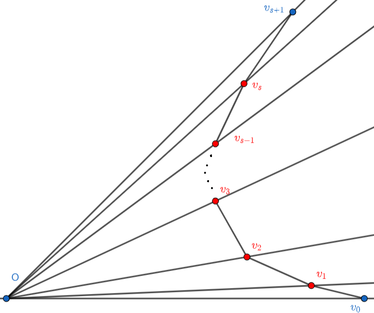
Figure 12. Resolved planar cone

Let us change the ${\mathbb{Z}}$-base of $N$ such that $e_{1}=v$ and $e_{2}=v_{0}$. So, we have $v_{s+1}=ne_{1}-qe_{2}$. We have,

$$\tau^{\vee}=C(e_{1},pe_{1}+ne_{2})\oplus\bigoplus_{i=3}^{d-3}{\mathbb{R}}w_{i}=C(w_{1},w_{2})\oplus{\mathbb{R}}^{d-2},$$

where the $w_{i}\in M$ are such that $\langle v_{0},w_{i}\rangle=\langle v_{s+1},w_{i}\rangle=0$ and $\langle\cdot,w\rangle\geq 0$ on $\tau$ for any $w\in C(w_{1},w_{2})$. Thus, in terms of toric varieties, $X_{\tau}=C_{q}\times({\mathbb{C}}^{\times})^{d-2}$, where $C_{q}=\mbox{Spec}({\mathbb{C}}[C(w_{1},w_{2})\cap M])$ is the cyclic quotient surface singularity of type $\frac{1}{n}(q,1)$ (Remark 2.25). Thus, the constructed resolution is a blow-up $h:\mbox{Bl}_{{\mathfrak{a}}}(X_{\tau})\to X_{\tau}$, where ${\mathfrak{a}}={\mathfrak{m}}\otimes{\mathbb{C}}[x_{3}^{\pm 1},...,x_{d}^{\pm 1}]$ and

$${\mathfrak{m}}=\bigoplus_{w\in C(w_{1},w_{2})\cap(M\setminus 0)}\chi^{m}.$$

For details see [CLS11, 11.3.6]. In particular, $\mbox{Bl}_{{\mathfrak{a}}}(X_{\tau})=\mbox{Bl}_{{\mathfrak{m}}}(X_{\tau})\times({\mathbb{C}}^{\times})^{d-2}$. We can give a explicit description of ${\mathfrak{m}}$ noting that the projection $C_{q}\to{\mathbb{A}}^{2}$ is given by the surjection ${\mathbb{C}}[\chi^{w_{1}},\chi^{w_{2}}]\to{\mathbb{C}}[C_{q}]$.

7.2. Dedekind sums

Consider the sawtooth function $((x))\colon{\mathbb{R}}\to{\mathbb{R}}$ is defined as

$$((x))=\left\{\begin{array}[]{cc}x-\lfloor x\rfloor-1/2&x\in{\mathbb{R}}\setminus{\mathbb{Z}}\\ 0&x\in{\mathbb{Z}}\end{array}\right..$$

Observe that is an odd periodic function of period $1$. For $n\geq 3$ prime and $a_{1},\ldots,a_{d}\in{\mathbb{Z}}$ define the Dedekind sum of dimension $d$ by

$$d(a_{1},\ldots,a_{d},n)=\sum_{i=1}^{n-1}\left(\left(\frac{ia_{1}}{n}\right)\right)\cdots\left(\left(\frac{ia_{d}}{n}\right)\right).$$

By periodicity, we can reduce $a_{i}\in{\mathbb{Z}}$ to $0\leq a_{i}<n$, then

$$d(a_{1},\ldots,a_{d},n)=d(\{a_{1}\}_{n},\ldots,\{a_{d}\}_{n},n).$$

where $\{a_{i}\}_{n}$ is the residue modulo $n$ of $a_{i}$. Since $((x))$ is an odd function, we always have

$$d(-a_{1},\ldots,-a_{d},n)=(-1)^{d}d(a_{1},\ldots,a_{d},n),\quad\forall x\in{\mathbb{Z}},\quad(x,n)=1,$$

i.e., $d(a_{1},...,a_{d},n)=0$ for any odd dimension $d$. Therefore, the non-trivial Dedekind sums are those of even dimension. We can rewrite this sum as

$$d(a_{1},\ldots,a_{d},n)=\frac{1}{n^{d}}\sum_{i=1}^{n-1}\left(\{ia_{1}\}_{n}-\frac{n}{2}\right)\cdots\left(\{ia_{d}\}_{n}-\frac{n}{2}\right).$$

Lemma 7.3.

We have the following relations,

$$\sum_{i=1}^{n-1}\{ia\}_{n}\{ib\}_{n}=n^{2}d(a,b,n)+\frac{n^{2}(n-1)}{4},$$

$$\sum_{i=1}^{n-1}\{ia\}_{n}^{2}\{ib\}_{n}=\sum_{i=1}^{n-1}\{ia\}_{n}\{ib\}_{n}^{2}=n^{3}d(a,b,n)+\frac{n^{2}(n-1)(2n-1)}{12}$$

$$\sum_{i=1}^{n-1}\{ia\}_{n}\{ib\}_{n}\{ic\}_{n}=\frac{n^{3}}{2}\left(d(a,b,n)+d(a,c,n)+d(b,c,n)\right)+\frac{n^{3}(n-1)}{8},$$

Proof.

We have an identity

$$\sum_{i=1}^{n-1}\{ia\}_{n}^{k}=\sum_{i=1}^{n-1}i^{k},$$

for each $k\geq 0$ integer. Then, we use repeatedly this identity in the following expressions. The first formula follows from,

$$n^{2}d(a,b,n)=\sum_{i=1}^{n-1}\left(\{ia\}_{n}-\frac{n}{2}\right)\left(\{ib\}_{n}-\frac{n}{2}\right),$$

and using that $0=\sum_{i=1}^{n-1}\left(\{ia\}_{n}-\frac{n}{2}\right)\left(\{ib\}_{n}-\frac{n}{2}\right)\left(\{ic\}_{n}-\frac{n}{2}\right),$ we get the other two.
∎

A well-known result due to Barkan [Bar77] (see Holzapfel [Hol88]) is the following formula relating the length $s$ of the continued fraction and Dedekind sums,

Proposition 7.4.

Let $n$ be a prime number, and $q$ be an integer such that $0<q<n$. Let $n/q=[k_{1},\ldots,k_{s}]$. Then $d(q,1,n)+s=\sum_{\alpha=1}^{s}(k_{\alpha}-2)+\frac{q+q^{\prime}}{n}.$

∎

Observe that from the above relation, and combining it with the results of Girstmair, we have an asymptotic behavior for the coefficients of the Hirzebruch-Jung continued fraction in the following sense: For a prime number $n\gg 0$, and integers $q\in O_{n}$ with $n/q=[k_{1},\ldots,k_{s}]$, we have $\sum_{\alpha=1}^{s}(k_{\alpha}-2)\leq 6\sqrt{n}+7$.

References

- [ABMMOG12] E. Artal-Bartolo, J. Martín-Morales, and J. Ortigas-Galindo. Intersection theory on abelian-quotient V-surfaces and -resolutions. Eleventh international conference Zaragoza-Pau on applied mathematics and statistics, Jaca, Spain, September 15–17, 2010., pages 13–23, 2012.
- [Ale94] Valery Alexeev. Boundness and for surfaces. International Journal of Mathematics, 5(06):779–810, 1994.
- [Ash15] T. Ashikaga. Toric modifications of cyclic orbifolds and an extended Zagier reciprocity for Dedekind sums. Tôhoku Math. J. (2), 67(3):323–347, 2015.
- [Ash19] T. Ashikaga. Multidimensional continued fractions for cyclic quotient singularities and Dedekind sums. Kyoto J. Math., 59(4):993–1039, 2019.
- [Bar77] P. Barkan. Sur les sommes de Dedekind et les fractions continues finies. C. R. Acad. Sci. Paris Sér. A-B, 284(16):A923–A926, 1977.
- [BCHM10] C. Birkar, P. Cascini, C. Hacon, and J. McKernan. Existence of minimal models for varieties of log general type. J. Am. Math. Soc., 23(2):405–468, 2010.
- [Bog78] F. Bogomolov. Holomorphic tensors and vector bundles on projective manifolds. Izv. Akad. Nauk SSSR Ser. Mat., 42:1227–1287, 1978.
- [BPS16] F. Bogomolov, A. Pirutka, and A. Silberstein. Families of disjoint divisors on varieties. Eur. J. Math., 2(4):917–928, 2016.
- [BS05] A. Buckley and B. Szendrői. Orbifold Riemann-Roch for threefolds with an application to Calabi-Yau geometry. J. Algebr. Geom., 14(4):601–622, 2005.
- [Buc08] Weronika Buczynska. Fake weighted projective spaces. arXiv: math.AG.0805.1211, 2008.
- [CH06] M. Chen and C. Hacon. On the geography of Gorenstein minimal 3-folds of general type. Asian J. Math., 10(4):757–763, 2006.
- [Cha97] M.-C. Chang. Distributions of Chern numbers of complete intersection threefolds. Geom. Funct. Anal., 7(5):861–872, 1997.
- [Cha99] M. Chang. On the density of ratios of Chern numbers of embedded threefolds. Commun. Algebra, 27(8):3771–3776, 1999.
- [Che87] Z. Chen. On the geography of surfaces - simply connected minimal surfaces with positive index. Math. Ann., 277:141–164, 1987.
- [Che91] Z. Chen. The existence of algebraic surfaces with preassigned Chern numbers. Math. Z., 206(2):241–254, 1991.
- [CL01] M. Chang and A. Lopez. A linear bound on the Euler number of threefolds of Calabi-Yau and of general type. Manuscr. Math., 105(1):47–67, 2001.
- [CLS11] T. Cox, J. Little, and H. Schenck. Toric Varieties, volume 124. AMS, Graduate Studies in Mathematics, 2011.
- [DS22] R. Du and H. Sun. Inequalities of Chern classes on nonsingular projective -folds with ample canonical or anti-canonical line bundles. J. Differ. Geom., 122(3):377–398, 2022.
- [EFU22] S. Eterović, F. Figueroa, and G. Urzúa. On the geography of line arrangements. Adv. Geom., 22(2):269–276, 2022.
- [Esn82] H. Esnault. Fibre de Milnor d’un cône sur une courbe plane singulière. Invent. Math., 68:477–496, 1982.
- [EV92] H. Esnault and E. Viehweg. Lectures on Vanishing Theorems, volume OWS 20. Birkhause Basel, 1992.
- [Ful93] W. Fulton. Introduction to toric varieties, volume 131. Princeton University Press, 1993.
- [Gao11] Y. Gao. A note on finite abelian covers. Sci. China, Math., 54(7):1333–1342, 2011.
- [Gir03] K. Girstmair. Zones of large and small values for Dedekind sums. Acta Arith., 109(3):299–308, 2003.
- [Gir06] K. Girstmair. Continued fractions and Dedekind sums: three-term relations and distribution. J. Number Theory, 119(1):66–85, 2006.
- [GKPT19] D. Greb, S. Kebekus, T. Peternell, and B. Taji. The Miyaoka-Yau inequality and uniformisation of canonical models. Ann. Sci. Éc. Norm. Supér. (4), 52(6):1487–1535, 2019.
- [Gre90] J. Greenfield. A proof for a quickhull algorithm. Electrical Engineering and Computer Science - Technical Reports. 65., 1990.
- [Har77] R. Hartshorne. Algebraic geometry, volume GTM 52. Springer, 1977.
- [Hir58] Friedrich Hirzebruch. Automorphe Formen und der Satz von Riemann-Roch. (Automorphic forms and the theorem of Riemann-Roch). Sympos. Int. Topologia Algebraica 129-144 (1958)., 1958.
- [Hir83] F. Hirzebruch. Arrangement of lines and algebraic surfaces. Progress in Math. Vol.II, 36:113–240, 1983.
- [Hol88] R.-P. Holzapfel. Chern number relations for locally abelian Galois coverings of algebraic surfaces. Math. Nachr., 138:263–292, 1988.
- [Hu18] Y. Hu. Inequality for Gorenstein minimal 3-folds of general type. Commun. Anal. Geom., 26(2):347–359, 2018.
- [Hun89] B. Hunt. Complex manifolds geography in dimension 2 and 3. J. Differential Geometry, 30:51–153, 1989.
- [Iit77] S. Iitaka. On logarithmic Kodaira dimension of algebraic varieties. Complex An.and Alg. Geom., pages 175–190, 1977.
- [Iit78] S. Iitaka. Geometry on complements of lines in . Tokyo J. Math., 1:1–19, 1978.
- [KM92] J. Kollár and S. Mori. Classification of three-dimensional flips. J. Am. Math. Soc., 5(3):533–703, 1992.
- [Kol91] J. Kollár. Flips, flops, minimal models, etc. Surveys in differential geometry. Vol. I, pages 113–199, 1991.
- [Kol23] J Kollár. Moduli of varieties of general type. Cambridge University Press, 2023.
- [KSB88] J. Kollár and N. I. Shepherd-Barron. Threefolds and deformations of surface singularities. Invent. Math., 91(2):299–338, 1988.
- [Laz04] R. Lazarsfeld. Positivity in algebraic geometry. I. Classical setting: line bundles and linear series, volume 48 of Ergeb. Math. Grenzgeb., 3. Folge. Berlin: Springer, 2004.
- [Liu97] Xianfang Liu. On the geography of threefolds. (With an appendix by Mei-Chu Chang). Tôhoku Math. J. (2), 49(1):59–71, appendix 69–71, 1997.
- [Mat10] K. Matsuki. Introduction to the Mori program. Universitext. Springer-Verlag, New York, 2010.
- [Miy77] Y. Miyaoka. On the Chern numbers of surfaces of general type. Invent. Math., 42:225–237, 1977.
- [Miy87] Y. Miyaoka. The pseudo-effectivity of for varieties with numerically effective canonical classes. Adv. Stud. Pure Math., 10:449––476, 1987.
- [Noe75] M. Noether. Zur theorie des eindeutigen entsprechends algebraischer gebilde. Math. Annalen, 2, 1875.
- [Par91] R. Pardini. Abelian covers of algebraic varieties. J. Reine Angew. Math., 417:191–213, 1991.
- [Per81] Ulf Persson. Chern invariants of surfaces of general type. Compos. Math., 43:3–58, 1981.
- [PSG94] A. N. Parshin, I. R. Shafarevich, and R. V. Gamkrelidze, editors. Algebraic geometry V: Fano Varieties, volume 55 of Encycl. Math. Sci. Berlin: Springer-Verlag, 1994.
- [Rei87] M. Reid. Young person’s guide to canonical singularities. Algebraic geometry, Proc. Summer Res. Inst., Brunswick/Maine 1985, part 1, Proc. Symp. Pure Math. 46, 345-414 (1987)., 1987.
- [RU15] X. Roulleau and G. Urzúa. Chern slopes of simply connected complex surfaces of general type are dense in [2,3]. Ann. of Math, Princeton (2), 182:287–306, 2015.
- [Som84] A. Sommese. On the density of ratios of chern numbers of algebraic surfaces. Math. Ann., 268:207–221, 1984.
- [Sta18] The Stacks Project Authors. Stacks Project. https://stacks.math.columbia.edu, 2018.
- [SXZ14] M. Sheng, J. Xu, and M. Zhang. On the Chern number inequalities satisfied by all smooth complete intersection threefolds with ample canonical class. Int. J. Math., 25(4):11, 2014. Id/No 1450029.
- [TU22] S. Troncoso and G. Urzúa. Savage surfaces. J. Eur. Math. Soc. (to appear), 2022.
- [Urz09] G. Urzúa. Algebraic surfaces and arrangements of curves. Journal of Algebraic Geometry, 19:169 – 189, 2009.
- [Urz16] G. Urzúa. Chern slopes of surfaces of general type in positive characteristic. Duke Math. J., 166:975–1004, 2016.
- [Vie77] E. Viehweg. Rational singularities of higher dimensional schemes. Proc. Am. Math. Soc., 63:6–8, 1977.
- [Vie82] E. Viehweg. Vanishing theorems. J. Reine Angew. Math., 335:1–8, 1982.
- [Yau77] S.-T. Yau. Calabi’s conjecture and some new results in algebraic geometry. Proc. Natl. Acad. Sci. USA, 74:1798–1799, 1977.