An Iterative Wavelet Threshold for Signal Denoising

This paper introduces an adaptive filtering process based on shrinking wavelet coefficients from the corresponding signal wavelet representation. The filtering procedure considers a threshold method determined by an iterative algorithm inspired by the control charts application, which is a tool of the statistical process control (SPC). The proposed method, called SpcShrink, is able to discriminate wavelet coefficients that significantly represent the signal of interest. The SpcShrink is algorithmically presented and numerically evaluated according to Monte Carlo simulations. Two empirical applications to real biomedical data filtering are also included and discussed. The SpcShrink shows superior performance when compared with competing algorithms.

Keywords
Adaptive filtering, Control chart, Signal denoising, Wavelet threshold

1 Introduction

Signal denosing is a classical problem in which a signal is measured in presence of additive white noise [41, 20]. In the past decades numerous contributions based on different approaches have been proposed for this problem. In [20], a list of methods is reviewed: signal denoising via learned dictionaries [20, 2], statistical estimators [23, 38], spatial adaptive filters [65, 43], stochastic analysis [21], partial differential equations [45], splines and other approximation theory methods [62], morphological analysis [57, 35], and transform-domain methods [63, 15, 60, 48, 41]. In this paper, we delimit the scope of our contribution to transform-domain filtering methods based on discrete wavelet transform (DWT) [14, 33, 41].

The DWT is widely regarded as a key tool in multi-resolution signal analysis [14, 33], signal detection [64, 7, 66], edge detection on images [34, 67], image compression [9], and signal denoising [17, 18, 9, 51, 47, 59], to mention a few applications in this field. Among its many possible applications, denoising techniques have been established as a major area of signal analysis [56], since data is often corrupted by noise during its acquisition or transmission.

Wavelet denoising techniques have been a staple of statistical functional estimation for years [36]. These techniques stem from the pioneer works by Donoho and collaborators [17, 18], where theoretical aspects concerning the application of wavelet transforms were introduced in this context. Some recent applications of wavelet denoising include: noise removal of biomedical signals [30], image denoising and compression [9], denoising of hyperspectral imagery [10], despeckling synthetic aperture radar image [49], smoothing of quantitative genomic data [25], anomaly detection for mine hunting [44], seismic noise attenuation [22], and noise reduction methods for chaotic signals [24]. In general, the central step in wavelet denoising techniques is the wavelet coefficient shrinkage [18]. This step consists of thresholding or shrinking the wavelet coefficients in the transform domain. In signal denoising via wavelet shrinkage, the threshold value selection is a critical step [11] with several methods for guiding the choice of the threshold value [51].

In this paper, we aim at proposing a new denoising scheme in the class of wavelet-transform methods. Indeed, we introduce an innovative approach for obtaining wavelet threshold values. The motivation for the proposed threshold value determination stems from control chart applications [55, 26, 6], which employ statistical process control (SPC) as a central tool [39]. Control charts are useful for determining whether a stochastic process is in the state of statistical control; being able to distinguish common and special variability causes [39]. Analogously, in the context of signal denoising, we are interested in identifying noise (common variability) and signal (special variability). Therefore, we refer to the sought method as SpcShrink. We introduce a sequence of control limits that allows iterative discarding of wavelet coefficients until all of them are within a specified control range. The threshold value keeps all coefficients inside the control range after successive limit estimations. In the SpcShrink formulation, instead of assuming constant variance for all wavelets coefficients as in [16], their exponential decay in different scales [11] is considered and explored in order to compute the desired threshold value.

The proposed method is presented and a numerical comparison with competing thresholding schemes in the literature is provided [17, 18, 9, 51]. Simulation results demonstrate the competitive performance of the proposed method. A computational quality measure assessment indicates the superiority of the proposed thresholding strategy when compared with popular methods. To emphasize the advantages of the proposed method, real biomedical noisy signals were filtered according to the SpcShrink. The obtained denoised signal has displayed significant feature preservation. At the same time, the SpcShrink is capable of efficiently discarding noise-related information.

This paper unfolds as follows. Section 2 summarizes the main concepts of wavelet shrinkage and SPC; then the proposed method is described. In Section 3, an optimization problem is solved to specify the optimal control limit distances for the proposed method. Numerical experiments are performed in Section 4, comparing the introduced method with classical and state-of-the-art wavelet thresholding schemes. For numerical evaluation we considered two real biomedical data and Monte Carlo simulations based on synthetic signals. Conclusions and final remarks are presented in Section 5.

2 SPC-based shrinkage

In this section, we present a short review on wavelet-based filtering. Then a summary of the main ideas behind statistical control charts and hypothesis test is also provided. Finally, by combining both tools in a straightforward manner, we introduce the SpcShrink method.

2.1 Review of wavelet shrinkage

Consider the problem of estimating an $N$-point unknown signal $\mathbf{x}=\begin{bmatrix}x[0]&x[1]&\cdots&x[N-1]\end{bmatrix}^{\top}$ from a set of $N$ noisy observations $\mathbf{y}=\begin{bmatrix}y[0]&y[1]&\cdots&y[N-1]\end{bmatrix}^{\top}$ furnished by:

$$\mathbf{y}=\mathbf{x}+\mathbf{n},$$ (1)

where $\mathbf{n}=\begin{bmatrix}n[0]&n[1]&\cdots&n[N-1]\end{bmatrix}^{\top}$ is a white Gaussian noise (WGN) vector with zero mean and variance $\sigma^{2}$ ($\mathcal{N}(0,\sigma^{2})$). In multiresolution wavelet analysis, we have $N=2^{J}$, where $J$ is the maximum number of wavelet decomposition levels [14, 33]. Let $\mathbf{W}$ be the orthonormal transformation matrix associated to a given multiresolution wavelet decomposition. Thus, the wavelet representation of $\mathbf{y}$ is given by:

$$\mathbf{w}=\mathbf{W}\cdot\mathbf{y}.$$

In a similar fashion, we denote $\mathbf{c}=\mathbf{W}\cdot\mathbf{x}$ and $\mathbf{z}=\mathbf{W}\cdot\mathbf{n}$. Because $\mathbf{W}$ is a linear transformation, the above quantities satisfy $\mathbf{w}=\mathbf{c}+\mathbf{z}$ (cf (1)). Additionally, the orthogonality of the discrete wavelet transform matrix ensures that $\mathbf{W}$ transforms white noise into white noise [18]. Thus, the transformed vector $\mathbf{z}$ is also WGN $\mathcal{N}(0,\sigma^{2})$.

For notational purposes, the entries of vectors $\mathbf{w}$, $\mathbf{c}$, and $\mathbf{z}$ are doubly indexed and denoted as $w_{j,k}$, $c_{j,k}$, and $z_{j,k}$, respectively, where $j=1,2,\ldots,J$ indicates the scaling domain (associated to frequency) index and $k=1,2,\ldots,2^{J-j}$ denotes the time domain index.

Wavelet shrinkage consists of a judicious thresholding operation over the elements of $\mathbf{w}$. Such operation results in a modified signal given by $\hat{\mathbf{w}}=T(\mathbf{w},\lambda)$, where $T(\cdot)$ is the thresholding function and $\lambda>0$ is the threshold value. Elements of $\mathbf{w}$ smaller than $\lambda$ are eliminated or smoothed [16, 9, 58]. Hard and soft thresholding are common strategies to ‘shrink’ wavelet coefficients [16, 9, 58] and the resulting wavelet coefficients $\hat{w}_{j,k}$ are, respectively, given by:

$$\hat{w}_{j,k}= \begin{cases}w_{j,k},&\text{if $|w_{j,k}|>\lambda$,}\\ 0,&\text{otherwise,}\end{cases}$$

$$\hat{w}_{j,k}= \begin{cases}\operatorname{sign}(w_{j,k})\cdot(w_{j,k}-\lambda),&\text{if $|w_{j,k}|>\lambda$,}\\ 0,&\text{otherwise,}\end{cases}$$

where $\operatorname{sign}(\cdot)$ is the signum function. Finally, the true signal can be estimated based on the shrunk coefficients according to $\hat{\mathbf{x}}=\mathbf{W}^{\top}\cdot\hat{\mathbf{w}}$ [40].

Threshold value $\lambda$ plays a central role in wavelet shrinkage denoising. Several methods for threshold estimation are described in literature, such as: the VisuShrink (or universal threshold) [17], the SureShrink [18], the BayesShrink [9], and the S-median [51]. Our goal is to propose an adaptive, level-dependent method for estimating $\lambda$ capable of high performance denoising and robust enough for hard or soft thresholding.

2.2 Review of control charts

Control charts are important statistical tools for monitoring disturbances in a statistical process, and they are richly applied in the industrial sector, the health sector and the agricultural sector, among others [55]. The main objective of control chart application is the identification of sources of variability in manufacturing processes [39, 46, 61, 31]. We propose the use of control charts theory as a means for threshold value estimation. A typical control chart consists of a time series of statistic measurements related to the quality characteristic of a given process. The chart contains a center line (CL) representing the mean value of the considered statistic and two horizontal lines, referred to as the lower control limit (LCL) and upper control limit (UCL).

Suppose normally distributed quality measurements with mean $\mu_{0}$ and standard deviation $\sigma$. If $\mathbf{y}=\begin{bmatrix}y[0]&y[1]&\cdots&y[N-1]\end{bmatrix}^{\top}$ is a vector with $N$ observations of this process, then the probability is $1-\alpha$ that any sample $y[i]$, with $i=0,1,\ldots,N-1$, falls within the following limits:

$$\mu_{0}-d\,\sigma,$$

$$\mu_{0}+d\,\sigma,$$

where $d$ is the ($1-\alpha/2$)-quantile of the standard normal distribution, or simply $d=\sqrt{2}\operatorname{erfc}^{-1}(\alpha)$, and $\operatorname{erfc}^{-1}(\cdot)$ is the inverse complementary error function [8, 5]. This way, the control limits are related according to [39]:

$$\mathrm{LCL}= \mu_{0}-d\,\sigma,$$ (2)

$$\mathrm{CL}= \mu_{0},$$ (3)

$$\mathrm{UCL}= \mu_{0}+d\,\sigma.$$ (4)

The quantity $d$ can also be interpreted as the “distance” of the control limits from its center line, expressed in standard deviation units. In control chart applications, $d$ is usually considered equal to three (three-sigma limits), where the probability of a simple point falling outside the limits is $0.0027$ [39, 46, 61, 31, 12]. In practice, quantities $\mu_{0}$ and $\sigma$ are statistically estimated.

There is a close connection between control charts and hypothesis testing [39, 31]. If the current value of $y[i]$ is within the control limits, then the process is considered to be ‘in control’; that is, it is an occurrence of a normal distributed variable with the mean value $\mu_{0}$. On the other hand, if $y[i]$ falls out the control limits, then we conclude that the process is ‘out of control’; that is, it is an occurrence from a random variable with a different mean value $\mu_{1}\neq\mu_{0}$. Therefore choosing the control limits is equivalent to setting up the critical region for testing the hypothesis [39]:

$$\begin{split}\mathcal{H}_{0}:&\,\mu=\mu_{0}\quad\text{(in control)},\\ \mathcal{H}_{1}:&\,\mu\neq\mu_{0}\quad\text{(out of control)}.\end{split}$$

The control chart tests this hypothesis repeatedly for each observation $y[i]$ of the observed process. The general procedure in hypothesis testing starts with the specification of type I error $\alpha$ (probability of false alarm), and then the design of a test procedure that maximizes the power of the test (probability of detection) [39]. Mathematically, we have $\alpha=\operatorname{Pr}(\text{reject $\mathcal{H}_{0}|\mathcal{H}_{0}$ is true})$ and $\text{Power}=\operatorname{Pr}(\text{reject $\mathcal{H}_{0}|\mathcal{H}_{0}$ is false})$. Then, by selecting $\alpha$, we directly control the probability of false alarm.

Practical SPC usage involves two phases [29]: (i) identification whether the system is in control and (ii) computation of the control limits to allow in-control identification. A system is regarded in control if most of its related measurements are within the control limits [46]. If a prescribed number of measurements is outside the range implied by LCL and UCL, then such outlying values are submitted to investigation or exclusion from the analysis set. If data are discarded, quantities CL, LCL, and UCL are recomputed and the cycle is repeated until all measurements are within control lines [39]. More details about the statistical analysis of SPC are found in [39], [46], [61], and [31].

2.3 Proposed SpcShrink

Control charts and wavelet shrinkage share similar goals: identifying and removing corrupted data—either out of control or noisy measurements. We aim at assessing each wavelet coefficient at a given decomposition level $j$ to establish whether it is representative of $\mathbf{x}$ or it is simply WGN $\mathbf{n}$. For such, we set up the following hypothesis test:

$$\begin{split}\mathcal{H}_{0}:&\,c_{j,k}=0,\\ \mathcal{H}_{1}:&\,c_{j,k}\neq 0.\end{split}$$ (5)

Notice that the null hypothesis is linked to noise only, whereas the alternative hypothesis indicates the presence of signal embedded in noise. Therefore, under the null hypothesis, we have $w_{j,k}=z_{j,k}$, which is WGN $\mathcal{N}(0,\sigma^{2})$ [18], as discussed in Section 2. The normality of the transformed noised data is an important property. In fact, it ensures the necessary conditions for the application of control chart theory over the wavelet domain, as discussed in Section 2.2. A similar statistical hypothesis formulation for the wavelet thresholding problem was considered in [1].

Based on the SPC approach, we assess the probability of a given wavelet coefficient $w_{j,k}$ being within the lower and upper limits based on (2), (3), and (4). Therefore, for each decomposition level $j$, we have that

$$\mathrm{LCL}= -d_{j}\cdot s_{j},$$

$$\mathrm{CL}= 0,$$

$$\mathrm{UCL}= d_{j}\cdot s_{j},$$

where $s_{j}$ is the corrected sample standard deviation of the wavelet coefficients at level $j$ and $d_{j}$ is distance of the control limits at level $j$. In this way, under the null-hypothesis $\mathcal{H}_{0}$, we have that

$$\operatorname{Pr}\{|w_{j,k}|\leq d_{j}\cdot s_{j}\}=1-\alpha_{j},$$

where $\alpha_{j}$ are the prescribed significance levels and $d_{j}=\sqrt{2}\operatorname{erfc}^{-1}(\alpha_{j})$. Indeed, the quantity $\alpha_{j}$ is the probability of detecting a signal when it is not present. For example, considering usual values for the significance level of $0.2\%$, $1\%$, $5\%$, and $10\%$ the implied values for the control limit distance $d_{j}$ are $3.09$, $2.58$, $1.96$, and $1.64$, respectively.

Thus, given a limit distance $d_{j}$, the proposed shrinkage method for estimating threshold values $\lambda_{j}$ at scale level $j$ is given by the iterative procedure described as follows:

1. Estimate the standard deviation of the wavelet coefficients at level $j$:

   $$s_{j}=\sqrt{\frac{1}{N_{j}-1}\sum_{k=1}^{N_{j}}(w_{j,k}-\bar{w}_{j}\,)^{2}},$$

   where $N_{j}=2^{J-j}$ is the number of wavelet coefficients at multi-resolution level $j$ and $\bar{w}_{j}=\frac{1}{N_{j}}\sum\limits_{k=1}^{N_{j}}w_{j,k}$.

2. Establish the control limits according to:

   $$\mathrm{LCL}= -d_{j}\cdot s_{j},$$

   $$\mathrm{UCL}= \;d_{j}\cdot s_{j},$$

   where $d_{j}=\sqrt{2}\operatorname{erfc}^{-1}(\alpha_{j})$ for the prescribed significance levels $\alpha_{j}$. Figure 1 illustrates the concept.

3. If a wavelet coefficient $w_{j,k}$, for $k=1,2,\ldots,N_{j}$, exceeds the control limits $[\mathrm{LCL},\mathrm{UCL}]$, then this coefficient is excluded and Steps 1) and 2) are repeated (Figure 1(b)). If all $w_{j,k}$ are inside the interval $[\mathrm{LCL},\mathrm{UCL}]$, then the threshold value is $\lambda_{j}=d_{j}\cdot s_{j}$ (Figures 1(b) and 1(c)) and the iterative method is stopped.

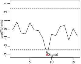
(a) Out of control coefficients ($s=0.93$)

(b) In control coefficients ($s=0.64$)

(c) Thresholded coefficients

Figure 1: Graphical illustration of the proposed iterative method.

It is a well-known fact that noise tends to be more pronounced at the lower scale levels and becomes less pronounced as the scale level $j$ increases [11]. Thus, as $j$ increases, the significance level $\alpha_{j}$ can also increase in value. The increase of the type I error probability $\alpha_{j}$ along the scales $j$ improves the probability of detection (power of test) of the hypothesis test described in (5). Therefore, in view of this behavior, the control limit distance must be adjusted accordingly. An increase in $\alpha_{j}$ effects a decrease in the value of the corresponding control limit distance $d_{j}$, because the function $\operatorname{erfc}^{-1}(\cdot)$ is a monotonically decreasing function over the interval $[0,1]$.

In a conservative fashion, we adopt a simple linear increase of $\alpha_{j}$ along the scales according to:

$$\alpha_{j}=j\cdot\alpha_{1},\quad j=2,3,\ldots,J_{0},$$

where $J_{0}\leq J$ is the number of decomposition levels and $\alpha_{1}$ is a statistical significance level to be determined. As a consequence, we have that the control limit distances are given by $d_{j}=\sqrt{2}\cdot\operatorname{erfc}^{-1}\left\{j\cdot\alpha_{1}\right\}$. Thus, because the proposed shrinkage method depends on the $\alpha_{1}$ value, we refer to it as SpcShrink($\alpha_{1}$). Thus, our proposed method has a free parameter in a similar way as the S-median method proposed by [51]. In the Section 3 we propose optimum values for $\alpha_{1}$.

2.4 Adaptivity and convergence

The proposed iterative method is adaptive in two senses: (i) it considers different threshold values for each wavelet decomposition level and (ii) based on control chart arguments, it discards detected signal samples and recalculates the threshold estimates, adapting itself to the signal characteristics.

The asymptotic convergence of the method is guaranteed. As it happens in statistical control charts, the SpcShrink can be understood as a heuristic to derive two sequences $\text{LCL}_{i}$ and $\text{UCL}_{i}$ being $\text{LCL}_{i}\leq\text{UCL}_{i}$, for each iteration $i$. For each iteration, these sequences are based on the computation of the mean value of the current data set, which is bounded by the maximum/minimum values of the data set. Each iteration discards some samples and the mean value is recomputed. This means the SpcShrink method, for each level $i$, generates two limited and monotonic sequences of real values; thus they must converge to a value when the number of iterations goes to infinity [32].

Let $J_{0}\leq J$ be the selected number of decomposition levels. For the algorithm introduced in Section 2.3, the numerical convergence is guaranteed. The main mathematical operations specifically required by the proposed algorithm are: (i) standard deviation computation (Step 1); (ii) evaluation of upper and lower control limits (Step 2); and (iii) element removal from a given array (Step 3). These operations require, respectively: $J_{0}$ calls per iteration; $J_{0}$ multiplications per iteration; and $J_{0}$ calls per iteration of find/sort algorithms which are computed in $\mathcal{O}(N\cdot\log N)$ by quicksort variants [13]. Indeed, in the worst case scenario, each iteration discards only a single wavelet coefficient. Since each decomposition level must keep at least one coefficient, the number of iterations is upper bound by $N-J_{0}$. Common to shrinkage algorithms, we have two calls (forward and inverse) of the particular wavelet transform at hand whose complexity is in $\mathcal{O}(N)$. Therefore, the proposed algorithm can be efficiently implemented in contemporary software packages at a very low computational cost.

3 Optimum specification of the control limit distances

The proposed method, as any hypothesis test, depends on the significance levels that define the control limit distances ($d_{j}$). In this section, we propose and solve an optimization problem to identify suitable values of a free parameter $\alpha_{1}$ that defines the limits $d_{j}=\sqrt{2}\cdot\operatorname{erfc}^{-1}\left\{j\cdot\alpha_{1}\right\}$. Computational and qualitative analyses are also presented.

3.1 Optimization problem

To obtain the optimal value for the significance levels, we introduce the following optimization problem:

$$\alpha_{1}^{\ast}=\arg\min_{\alpha_{1}\in A}\frac{1}{M}\sum_{i=1}^{M}\operatorname{Error}(\mathbf{x}_{i},\hat{\mathbf{x}}_{i}),$$ (6)

where $\mathbf{x}_{i}$ is an input signal, $\hat{\mathbf{x}}_{i}$ is the associated denoised signal according to the proposed scheme, $\operatorname{Error}(\cdot,\cdot)$ is a figure of merit to assess the denoised signal, $M$ is the number of signal instantiations, and $\mathcal{A}$ is the search space. For the error measure $\operatorname{Error}$, we adopted the negative value of the classical signal-to-noise ratio (SNR). This measure is defined by

$$\operatorname{SNR}(\mathbf{x}_{i},\hat{\mathbf{x}}_{i})=10\log_{10}\left(\frac{\sigma^{2}_{\text{signal}}}{\sigma^{2}_{\text{noise}}}\right),$$ (7)

where $\sigma^{2}_{\text{signal}}$ is the variance of the $\mathbf{x}_{i}$ and $\sigma^{2}_{\text{noise}}$ is the variance of $\mathbf{x}_{i}-\hat{\mathbf{x}}_{i}$. In practice, variance estimates are considered. The SNR is given in decibels (dB), where greater SNR value indicate better filtering.

3.2 Computational search

(a) Blocks

(b) Bumps

(c) Doppler

Figure 2: Standardized signals used in the proposed numerical evaluations.

Figure 3: Quantitative SpcShrink($\alpha_{1}$) comparison considering several $\alpha_{1}$ values for different levels of corrupted signal (in dB).

In order to solve (6), we set up a Monte Carlo simulation [19, 54]. For input data, we separated the signals depicted in Figure 2. These are standard signals largely employed for assessing filtering processes as shown in [18, 17] and [27]. The selected signal blocklength was $2^{12}$ points. As suggested in [9] and [51], we adopted the Daubechies wavelet with eight vanishing moments [14] as the analyzing wavelet. Five scales ($J_{0}=5$) were considered in the orthogonal wavelet decomposition and soft thresholding was employed. Considering $M=1500$ replications of the standard signals, 500 instantiations for each signal shown in Figure 2, we submitted them to additive WGN with different variances $\sigma^{2}_{\text{noise}}$ resulting in the following SNR: 5, 15, 25, and 35 dB, according to (7).

We adopted the following search space: $\mathcal{A}=\{0.1\%,0.2\%,0.3\%,\ldots,4.9\%,5\%\}$. The resulting denoised signals were assessed by means of SNR measurements. Results were averaged and the numerical minimum was sought (cf. (6)). Figure 3 displays SNR plots over $\mathcal{A}$. For each considered noise level, a different value of $\alpha_{1}^{\ast}$ was obtained. The obtained minima are shown in Table 1. Because the quantity $\alpha_{1}^{\ast}$ varies according to the injected noise level, we computed the average of the minima. Hereafter, we refer to such average value simply as $\alpha_{1}$. Thus, we identified the mean value $\alpha_{1}=1.5\%$ that represent a good compromise solution for all considered scenarios. For $\alpha_{1}=1.5\%$ the control limit distances are $d_{1}=2.432$, $d_{2}=2.170$, $d_{3}=2.005$, $d_{4}=1.881$, and $d_{5}=1.780$.

Table 1: Optimal parameters $\alpha_{1}^{\ast}$

Noise level	$5$ dB	$15$ dB	$25$ dB	$35$ dB	Mean
$\alpha_{1}^{\ast}$	1.1	1.4	1.7	1.8	1.5

3.3 Qualitative analysis

(a) Input blocks signal with 20 dB

(b) Input bumps signal with 20 dB

(c) Input Doppler signal with 20 dB

(d) $\alpha_{1}\!=\!5\%$ (SNR=24.17)

(e) $\alpha_{1}\!=\!5\%$ (SNR=24.13)

(f) $\alpha_{1}\!=\!5\%$ (SNR=22.92)

(g) $\alpha_{1}\!=\!2.5\%$ (SNR=26.24)

(h) $\alpha_{1}\!=\!2.5\%$ (SNR=26.97)

(i) $\alpha_{1}\!=\!2.5\%$ (SNR=25.65)

(j) $\alpha_{1}\!=\!1.5\%$ (SNR=26.61)

(k) $\alpha_{1}\!=\!1.5\%$ (SNR=27.28)

(l) $\alpha_{1}\!=\!1.5\%$ (SNR=25.63)

(m) $\alpha_{1}\!\!=\!\!1.0\%$ (SNR=25.57)

(n) $\alpha_{1}\!=\!1.0\%$ (SNR=26.37)

(o) $\alpha_{1}\!=\!1.0\%$ (SNR=25.03)

(p) $\alpha_{1}\!=\!0.1\%$ (SNR=22.46)

(q) $\alpha_{1}\!=\!0.1\%$ (SNR=22.97)

(r) $\alpha_{1}\!=\!0.1\%$ (SNR=22.31)

Figure 4: Output filtered signal comparison by SpcShrink($\alpha_{1}$) with several $\alpha_{1}$ values.

Filtering methods that minimize a quantitative measure, such as SNR or mean square error, do not necessarily lead in better image visual quality results in the sense described by [15], [16], and [17]. As an example, the VisuShrink [17] provides better visual quality than procedures based on mean square error minimization [16]. Therefore, we examined the behavior of the proposed method at the vicinity of the optimal value $\alpha=1.5\%$. The goal is to probe for resulting signals which display good visual quality after wavelet coefficient shrinkage.

Figure 4 shows a qualitative analysis of the denoised signals according to the proposed method for noisy signals with SNR of 20 dB and several values of $\alpha_{1}$. Notice that for $\alpha_{1}=1.5\%$, in general, the discussed thresholding yielded higher SNR output signal. On the other hand, the case where $\alpha_{1}=1.0\%$ provides better visual result. Similar to VisuShrink, SpcShrink($1.0\%$) furnishes outputs with smooth visual appearance at a lower SNR. We note that as the value of $\alpha_{1}$ decreases the output signal becomes smoother.

The proposed method is capable of trading-off quantitative measurements (e.g., SNR) for smoothness (cf. VisuShrink [17]). Such balancing is not available in traditional wavelet shrinkage methods, such as VisuShrink, SureShrink, and BayesShrink.

4 Numerical comparisons

In this section we aim at comparing the proposed method with the following well-known shrinkage schemes: VisuShrink [17], SureShrink [18], BayesShrink [9], and S-median [51]. For the introduced scheme, we selected the control limit distances associated to $\alpha_{1}\in\{1.0\%,1.5\%\}$, because these values of $\alpha_{1}$ were demonstrated to lead to useful results as described in the previous section.

We present computational experiments to assess the performance of the proposed SpcShrink($\alpha_{1}$) filtering process in two scenarios: (i) synthetic signals (Section 4.1) and (ii) actual biomedical data (Section 4.2). For data in Scenario (i), we evaluated the influence of the noise level in denoising techniques by means of Monte Carlo simulations. Additionally, the impact of changing the wavelet filter length is also stressed in this section. In Scenario (ii), we also include a visual quality assessment of the filtered data, since this is a relevant aspect in applications involving actual biomedical signals [4]. All computations were performed in the R programming language [52].

4.1 Synthetic data denosing

(a) Blocks

(b) Bumps

(c) Doppler

Figure 5: SNR measures comparison of different thresholding for several noise level.

(a) Blocks

(b) Bumps

(c) Doppler

Figure 6: Quantitative noise suppression analysis of different thresholding in SNR gain.

(a) Blocks

(b) Bumps

(c) Doppler

Figure 7: RMSE measures comparison of different thresholding for several noise levels.

Firstly, to assess the signal denoising performance, the SNR was employed as figure of merit. As considered in [51], we also employed the root mean square error (RMSE) for this evaluation. SNR and RMSE values were computed in average; considering 1,000 replications of the described Monte Carlo simulation. For this simulation we adopted the Daubechies wavelet with eight vanishing moments and five scales ($J_{0}=5$). The selected blocklength of the signals in Figure 2 was $2^{12}$ points. Following an approach similar to the one described in [51], we fixed the WGN levels to signals with input SNR varying from 5 dB to 35 dB in steps of 1 dB, as shown in Figures 5 and 7. Thus, we considered three benchmarking signals, additive WGN under 31 different variance levels, and 1,000 Monte Carlo replications, totalizing $(3\times 31\times 1,000)=93,000$ simulated signals in our validation experiments.

Considering the SNR results presented in Figure 5, the proposed scheme outperforms the competing methods in almost every analyzed scenarios, except for the ‘Doppler’ input signal with noise level smaller than 10 dB. For the ‘blocks’ and ‘bumps’ signals the SpcShrink(1.5%) furnished best results, whereas for the ‘Doppler’ signal the SpcShrink(1.0%) is recommended. As suggested in [4], we also considered the SNR gain of the proposed method. The SNR gain is the difference between the output SNR and input SNR values. Therefore, the SNR gain can quantify the noise suppression. Figure 6 shows the results. The proposed method achieves the highest gains in almost all considered scenarios. In particular, gains of more than 12 dB could be attained when the input SNR is lower than 10 dB.

Table 2: SNR comparison of the wavelet denoising methods with different scales ($J_{0}$) in wavelet decomposition for some corrupted signals

Signal	​​​​ Input SNR	​​​​VisuShrink	​​​​SureShrink	​​​​ S-median	​​​​ BayesShrink	​​​​​ SpcShrink(1.0%)	​​​​​ SpcShrink(1.5%)
$J_{0}=3$
	$10$	$16.9284$	$17.1682$	$17.1529$	$17.3786$	$\mathbf{17.5157}$	$17.4955$
Blocks	$20$	$23.6527$	$23.4104$	$25.8875$	$25.6691$	$25.8675$	$\mathbf{26.1224}$
	$30$	$31.4303$	$30.7546$	$34.9138$	$32.5868$	$34.7118$	$\mathbf{35.1352}$
	$10$	$16.6927$	$16.6328$	$17.0943$	$17.5152$	$17.5620$	$\mathbf{17.5748}$
Bumps	$20$	$23.9173$	$23.5005$	$25.9814$	$25.6219$	$26.1922$	$\mathbf{26.4381}$
	$30$	$31.7294$	$31.0382$	$35.0473$	$33.6996$	$34.9675$	$\mathbf{35.3802}$
	$10$	$18.7457$	$18.7465$	$18.0588$	$\mathbf{18.7533}$	$18.6386$	$18.4332$
Doppler	$20$	$27.7186$	$27.7476$	$27.7750$	$28.3486$	$\mathbf{28.3698}$	$28.2441$
	$30$	$36.9345$	$36.9477$	$37.4739$	$36.9797$	$\mathbf{38.0408}$	$37.9911$
$J_{0}=5$
	$10$	$15.5543$	$17.7555$	$17.5772$	$18.6515$	$18.4976$	$\mathbf{18.8388}$
Blocks	$20$	$21.6718$	$22.0240$	$25.7155$	$26.0159$	$26.0451$	$\mathbf{26.7315}$
	$30$	$29.6308$	$28.0889$	$34.5558$	$32.6437$	$34.6019$	$\mathbf{35.4334}$
	$10$	$14.1192$	$14.2867$	$17.0311$	$18.2352$	$18.0367$	$\mathbf{18.5925}$
Bumps	$20$	$21.3501$	$19.4759$	$25.5057$	$25.7783$	$26.1079$	$\mathbf{26.8944}$
	$30$	$29.5557$	$27.0169$	$34.4599$	$33.7318$	$34.6840$	$\mathbf{35.5688}$
	$10$	$19.9791$	$20.2527$	$20.1582$	$21.8216$	$\mathbf{21.9260}$	$21.3008$
Doppler	$20$	$27.3108$	$27.6216$	$29.3106$	$29.5763$	$\mathbf{30.8778}$	$30.6738$
	$30$	$35.7908$	$36.0083$	$38.5994$	$37.2800$	$39.9721$	$\mathbf{40.0392}$
$J_{0}=7$
	$10$	$13.6838$	$17.6491$	$16.8629$	$\mathbf{18.7340}$	$17.1242$	$18.4060$
Blocks	$20$	$20.4336$	$21.4884$	$25.1580$	$26.0295$	$24.7394$	$\mathbf{26.3133}$
	$30$	$28.6483$	$26.2480$	$34.0793$	$32.6455$	$32.7050$	$\mathbf{34.6061}$
	$10$	$12.2659$	$13.5925$	$16.2727$	$\mathbf{18.2628}$	$15.4125$	$18.1198$
Bumps	$20$	$20.0665$	$17.7032$	$24.9131$	$\mathbf{25.7825}$	$21.8971$	$25.6458$
	$30$	$28.5332$	$20.9340$	$\mathbf{33.9617}$	$33.7325$	$25.4695$	$31.1702$
	$10$	$18.1128$	$18.7434$	$19.9863$	$22.1059$	$\mathbf{22.4194}$	$21.8497$
Doppler	$20$	$25.7923$	$25.7641$	$29.0273$	$29.6304$	$\mathbf{31.0512}$	$31.0435$
	$30$	$34.4638$	$34.2910$	$38.3058$	$37.2898$	$40.0073$	$\mathbf{40.2910}$

In addition to SNR measurements, we also included RMSE results shown in Figure 7. The proposed method could outperform the competing methods for a wide range of input SNR (greater than 10 dB). It could also surpass the well-known VisuShrink and SureShrink for all values of input SNR. For ‘blocks’ and ‘Doppler’ signals, at lower than 10 dB input SNR, the BayesShrink performed slightly better (less than 3.3% better). In the majority of the simulation scenarios, the S-median produced better results than the VisuShrink scheme. This is expected since S-median is a level-dependent version of the VisuShrink [51].

In terms of computational costs, for the above simulation results, the SpcShrink(1.0%) required a number of iterations ranging from 30 to 46; whereas the SpcShrink(1.0%) required from 45 to 56 iterations.

We considered a second methodology for assessing the performance of the wavelet threshold methods. Now, we evaluated the SNR measures for each prototype signal at three different scales in the multiresolution analysis, namely: $J_{0}=3$, $J_{0}=5$, and $J_{0}=7$. We also considered three WGN levels, 1,000 Monte Carlo replications, Daubechies wavelet with eight vanishing moments, and signals with $2^{12}$ samples. Results are presented in Table 2 in a similar fashion of [37]. The best results are highlighted in bold.

Table 2 shows a superior performance of the SpcShrink, specially with $\alpha_{0}=1.5\%$. For $J_{0}=3$ and $J_{0}=5$, we note that the proposed method achieves the best results in almost all cases. For $J_{0}=7$, the results are still good, keeping the majority of the best figures. We note that even when the SpcShrink does not achieve the best SNR measures, it is among the three best results. In summary, Table 2 brings evidence that the proposed method is robust even when operating at different scales ($J_{0}$) of wavelet decomposition analysis.

4.2 Biomedical signal denoising

In order to illustrate the potential of the proposed SpcShrink as a denoising procedure, we consider two actual biomedical signals, namely: (i) an inductance plethysmography data (IPD), and (ii) an electrocardiogram (ECG). Fig. 8 shows these signals.

(a) Original real IPD

(b) Original real ECG

Figure 8: Biomedical signals considered in denoising experiments.

Firstly, we submitted $2^{12}$ samples of IPD to the denoising methods. Such data was acquired in the context of patient breathing after general anesthesia; being available in [42]. This particular signal was previously described in [40] and was also considered in benchmark tests in [28] and [53]. Figure 9 displays the filtered signal according to the considered methods. For these results, the proposed methods SpcShrink(1.0%) and SpcShrink(1.5%) demanded only 40 and 56 iterations for convergence, respectively. We note that the proposed algorithm is capable of removing noise and preserving the general shape of the signal as well as its peak intensities and periodicities, which are significant characteristics to be retained in a denoised signal [4].

(a) Filtered by the VisuShrink

(b) Filtered by the SureShrink

(c) Filtered by the S-median

(d) Filtered by the BayesShrink

(e) Filtered by the SpcShrink($1.5\%$)

(f) Filtered by the SpcShrink($1.0\%$)

Figure 9: Filtered inductance plethysmography data (IPD) by several methods.

Secondly, we considered $2^{11}$ samples of an ECG signal. Observations sampled from a patient with arrhythmia over an interval of 11.37 seconds at a sampling frequency of 180 Hz. This data is available in [3]. For more detailed information regarding this data, see [50, p. 125]. In Fig. 10 the filtered signals are presented. In this application, the SpcShrink(1.0%) and SpcShrink(1.5%) demanded only 51 and 52 iterations for convergence, respectively. We note that SureShrink flattened the picks of the QRS complex. The methods S-median and BayesShrink maintain the most part of the noise in the signal. Results derived from VisuShrink and the proposed method are comparable balancing noise reduction and shape of the ECG signal.

(a) Filtered by the VisuShrink

(b) Filtered by the SureShrink

(c) Filtered by the S-median

(d) Filtered by the BayesShrink

(e) Filtered by the SpcShrink($1.5\%$)

(f) Filtered by the SpcShrink($1.0\%$)

Figure 10: Filtered electrocardiogram (ECG) signal by several methods.

In the discussed biomedical signal processing, the SpcShrink showed similar visual performance when compared to the VisuShrink. In ECG filtering the SureShrink showed poor results, whereas it offered good visual quality for IPD denoising. Regarding to S-median and BayesShrink methods, despite their good performances in the quantitative analysis, as described in Subsection 4.1, the resulting signals present visible fine scale roughness. On the other hand, the proposed method excels both in quantitative analysis, by maximizing SNR gains (cf. Section 4.1) and, in visual analysis, by effecting smooth signals. This good performance in both analyses is due to the strong adaptive trait present in the proposed method, which is capable of discriminating noise (common cause) from signal (special cause) in an iterative way.

5 Conclusions

In this work a new signal denoising scheme, called SpcShrink, was proposed. The introduced method was inspired by the control charts application and based on wavelet shrinkage, inheriting its own mathematical justifications from the SPC method. Iterative search procedures for establishing the statistical control state motivated the search for appropriate threshold values, which is the main shrinkage step. The SpcShrink depends on a free parameter $(\alpha_{1})$ which allows for a trade-off between quantitative error measurements and visual quality of filtered signals. Based on an optimization problem and Monte Carlo simulations results, we suggest $\alpha_{1}=1.5\%$ for SNR gain maximization and $\alpha_{1}=1.0\%$ for better visual quality. The proposed method was assessed in a Monte Carlo simulation, with SNR, SNR gain, and RMSE as figures of merit. Then it was compared with several popular shrinkage schemes, considering a variety of test signals and different input noise levels. In addition to the good visual performance, quantitative results are favorable to the proposed shrinkage method, which could outperform VisuShrink, SureShrink, BayesShrink, and S-median in various scenarios.

References

- [1] F. Abramovich and Y. Benjamini, Adaptive thresholding of wavelet coefficients, Computational Statistics & Data Analysis, 22 (1996), pp. 351–361.
- [2] M. Aharon, M. Elad, and A. Bruckstein, K-SVD: An algorithm for designing overcomplete dictionaries for sparse representation, IEEE Transactions on Signal Processing, 54 (2006), pp. 4311–4322.
- [3] E. Aldrich, wavelets: A package of functions for computing wavelet filters, wavelet transforms and multiresolution analyses, 2013. R package version 0.3-0.
- [4] A. Aldroubi and M. Unser, Wavelets in Medicine and Biology, Taylor & Francis, 1996.
- [5] L. Andrews, Special Functions of Mathematics for Engineers, Oxford Science Publications, SPIE Optical Engineering Press, 1997.
- [6] W. Arshad, N. Abbas, M. Riaz, and Z. Hussain, Simultaneous use of runs rules and auxiliary information with exponentially weighted moving average control charts, Quality and Reliability Engineering International, 33 (2017), pp. 323–336.
- [7] T. C. Bailey, T. Sapatinas, K. J. Powell, and W. J. Krzanowski, Signal detection in underwater sound using wavelets, Journal of the American Statistical Association, 93 (1998), pp. 73–83.
- [8] L. Carlitz, The inverse of the error function, Pacific Journal of Mathematics, 13 (1963), pp. 459–470.
- [9] S. G. Chang, B. Yu, and M. Vetterli, Adaptive wavelet thresholding for image denoising and compression, IEEE Transactions on Image Processing, 9 (2000), pp. 1532–1546.
- [10] G. Chen and S.-E. Qian, Denoising of hyperspectral imagery using principal component analysis and wavelet shrinkage, IEEE Transactions on Geoscience and Remote Sensing, 49 (2011), pp. 973–980.
- [11] Y. Chen and C. Han, Adaptive wavelet threshold for image denoising, Electronics Letters, 41 (2005).
- [12] G. E. Cook, J. E. Maxwell, R. J. Barnett, and A. M. Strauss, Statistical process control application to weld process, IEEE Transactions on Industry Applications, 33 (1997), pp. 454–463.
- [13] T. H. Cormen, C. E. Leiserson, R. L. Rivest, and C. Stein, Introduction to Algorithms, MIT Press, 3 ed., 2009.
- [14] I. Daubechies, Ten lectures on wavelets, Society for Industrial and Applied Mathematics, 1992.
- [15] D. Donoho and I. Johnstone, Threshold selection for wavelet shrinkage of noisy data, in Proceedings of the 16th Annual International Conference of the IEEE. Engineering Advances: New Opportunities for Biomedical Engineers., 1994, pp. A24–A25 vol.1.
- [16] D. L. Donoho, De-noising by soft-thresholding, IEEE Transactions on Information Theory, 41 (1995), pp. 613–627.
- [17] D. L. Donoho and I. M. Johnstone, Ideal spatial adaptation via wavelet shrinkage, Biometrika, 81 (1994), pp. 425–455.
- [18] , Adapting to unknown smoothness via wavelet shrinkage, Journal of the American Statistical Association, 90 (1995), pp. 1200–1224.
- [19] A. Doucet and X. Wang, Monte Carlo methods for signal processing: a review in the statistical signal processing context, IEEE Signal Processing Magazine, 22 (2005), pp. 152–170.
- [20] M. Elad and M. Aharon, Image denoising via sparse and redundant representations over learned dictionaries, IEEE Transactions on Image Processing, 15 (2006), pp. 3736–3745.
- [21] S. H. Fouladi, M. Hajiramezanali, H. Amindavar, J. A. Ritcey, and P. Arabshahi, Denoising based on multivariate stochastic volatility modeling of multiwavelet coefficients, IEEE Transactions on Signal Processing, 61 (2013), pp. 5578–5589.
- [22] A. Goudarzi and M. A. Riahi, Seismic coherent and random noise attenuation using the undecimated discrete wavelet transform method with WDGA technique, Journal of Geophysics and Engineering, 9 (2012), pp. 619–631.
- [23] A. B. Hamza and H. Krim, Image denoising: a nonlinear robust statistical approach, IEEE Transactions on Signal Processing, 49 (2001), pp. 3045–3054.
- [24] X. Han and X. Chang, An intelligent noise reduction method for chaotic signals based on genetic algorithms and lifting wavelet transforms, Information Sciences, 218 (2013), pp. 103 – 118.
- [25] H. Hatsuda, Robust smoothing of quantitative genomic data using second-generation wavelets and bivariate shrinkage, IEEE Transactions on Biomedical Engineering, 59 (2012), pp. 2099–2102.
- [26] M. P. Hossain, M. H. Omar, and M. Riaz, New V control chart for the Maxwell distribution, Journal of Statistical Computation and Simulation, 87 (2017), pp. 594–606.
- [27] C. M. Hurvich and C.-L. Tsai, A crossvalidatory AIC for hard wavelet thresholding in spatially adaptive function estimation, Biometrika, 85 (1998), pp. 701–710.
- [28] I. M. Johnstone and B. W. Silverman, Empirical bayes selection of wavelet thresholds, The Annals of Statistics, 33 (2005), pp. 1700–1752.
- [29] L. A. Jones and C. W. Champ, Phase I control charts for times between events, Quality and Reliability Engineering International, 18 (2002), pp. 479–488.
- [30] A. Kozakevicius, C. Rodrigues, R. Nunes, and R. Guerra-Filho, Adaptive ECG filtering and QRS detection using orthogonal wavelet transform, in Proceedings of International Conference on BioMedical Engineering (IASTED), Austria, 2005, Innsbruck.
- [31] T. M. Kubiak and D. W. Benbow, The Certified Six Sigma Black Belt Handbook, ASQ Quality Press, 2 ed., 2009. p. 648.
- [32] M. Laczkovich and V. T. Sós, Real Analysis: Foundations and Functions of One Variable, Springer, 2015.
- [33] S. G. Mallat, A Wavelet Tour of Signal Processing, Academic Press, 3 ed., 2008.
- [34] S. G. Mallat and W.-L. Hwang, Singularity detection and processing with wavelets, IEEE Transactions on Information Theory, 38 (1992), pp. 617–643.
- [35] P. Maragos, R. W. Schafer, and M. A. Butt, Mathematical Morphology and Its Applications to Image and Signal Processing, Springer, 1996.
- [36] K. McGinnity, R. Varbanov, and E. Chicken, Cross-validated wavelet block thresholding for non-Gaussian errors, Computational Statistics & Data Analysis, 106 (2017), pp. 127 – 137.
- [37] A. Mert and A. Akan, Detrended fluctuation thresholding for empirical mode decomposition based denoising, Digital Signal Processing, 32 (2014), pp. 48 – 56.
- [38] A. Montanari, Statistical Physics, Optimization, Inference, and Message-Passing Algorithms, Oxford Scholarship, 2015, ch. Statistical estimation: from denoising to sparse regression and hidden cliques.
- [39] D. C. Montgomery, Introduction to Statistical Quality Control, John Wiley & Sons, Inc., 6 ed., 2009.
- [40] G. P. Nason, Wavelet shrinkage using cross-validation, Journal of the Royal Statistical Society. Series B, 58 (1996), pp. 463–479.
- [41] G. P. Nason, Wavelet Methods in Statistics with R, Springer, 2011.
- [42] G. P. Nason, wavethresh: Wavelets statistics and transforms., 2013. R package version 4.6.6.
- [43] V. D. Navarro-Sanchez and J. M. Lopez-Sanchez, Spatial adaptive speckle filtering driven by temporal polarimetric statistics and its application to PSI, IEEE Transactions on Geoscience and Remote Sensing, 52 (2014), pp. 4548–4557.
- [44] J. Nelson and N. Kingsbury, Fractal dimension, wavelet shrinkage and anomaly detection for mine hunting, IET Signal Processing, 6 (2012), pp. 484–493.
- [45] O. Niang, A. Thioune, M. C. E. Gueirea, E. Delechelle, and J. Lemoine, Partial differential equation-based approach for empirical mode decomposition: Application on image analysis, IEEE Transactions on Image Processing, 21 (2012), pp. 3991–4001.
- [46] J. S. Oakland, Statistical Process Control, Routledge, 6 ed., 2007.
- [47] H.-S. Oh, D. Kim, and Y. Kim, Robust wavelet shrinkage using robust selection of thresholds, Statistics and Computing, 19 (2009), pp. 27–34.
- [48] A. V. Oppenheim and R. W. Schafer, Discrete-Time Signal Processing, Pearson, 2009.
- [49] S. Parrilli, M. Poderico, C. V. Angelino, and L. Verdoliva, A nonlocal SAR image denoising algorithm based on LLMMSE wavelet shrinkage, IEEE Transactions on Geoscience and Remote Sensing, 50 (2012), pp. 606–616.
- [50] D. B. Percival and A. T. Walden, Wavelet Methods for Time Series Analysis, Cambridge University Press, 2000.
- [51] S. Poornachandra, Wavelet-based denoising using subband dependent threshold for ECG signals, Digital Signal Processing, 18 (2008), pp. 49–55.
- [52] R Core Team, R: A Language and Environment for Statistical Computing, R Foundation for Statistical Computing, Vienna, Austria, 2018.
- [53] N. Remenyi and B. Vidakovic, Lambda-neighborhood wavelet shrinkage, Computational Statistics & Data Analysis, 57 (2013), pp. 404–416.
- [54] M. L. Rizzo, Statistical Computing with R, Chapman and Hall, 2007. p. 416.
- [55] R. A. Sanusi, M. R. Abujiya, M. Riaz, and N. Abbas, Combined Shewhart CUSUM charts using auxiliary variable, Computers & Industrial Engineering, 105 (2017), pp. 329–337.
- [56] A. Singer, Y. Shkolnisky, and B. Nadler, Diffusion interpretation of nonlocal neighborhood filters for signal denoising, SIAM Journal on Imaging Sciences, 2 (2009), pp. 118–139.
- [57] B. N. Singh and A. K. Tiwari, Optimal selection of wavelet basis function applied to ECG signal denoising, Digital Signal Processing, 16 (2006), pp. 275–287.
- [58] C. B. Smith, S. Agaian, and D. Akopian, A wavelet-denoising approach using polynomial threshold aperators, IEEE Signal Processing Letters, 15 (2008), pp. 906–909.
- [59] M. Srivastava, C. L. Anderson, and J. H. Freed, A new wavelet denoising method for selecting decomposition levels and noise thresholds, IEEE Access, 4 (2016), pp. 3862–3877.
- [60] J.-L. Starck, E. J. Candes, and D. L. Donoho, The curvelet transform for image denoising, IEEE Transactions on Image Processing, 11 (2002), pp. 670–684.
- [61] N. R. Tague, The Quality Toolbox, ASQ Quality Press, 2 ed., 2005. p. 584.
- [62] M. Unser, Splines: a perfect fit for signal and image processing, IEEE Signal Processing Magazine, 16 (1999), pp. 22–38.
- [63] M. Vetterli and C. Herley, Wavelets and filter banks: theory and design, IEEE Transactions on Signal Processing, 40 (1992), pp. 2207–2232.
- [64] Y. Wang, Jump and sharp cusp detection by wavelets, Biometrika, 82 (1995), pp. 385–397.
- [65] H. Woehrle, M. M. Krell, S. Straube, S. K. Kim, E. A. Kirchner, and F. Kirchner, An adaptive spatial filter for user-independent single trial detection of event-related potentials, IEEE Transactions on Biomedical Engineering, 62 (2015), pp. 1696–1705.
- [66] Y. Xue, R. Gençay, and S. Fagan, Jump detection with wavelets for high-frequency financial time series, Quantitative Finance, 14 (2014), pp. 1427–1444.
- [67] Z. Zhang, S. Ma, H. Liu, and Y. Gong, An edge detection approach based on directional wavelet transform, Computers & Mathematics with Applications, 57 (2009), pp. 1265 – 1271.