A Basic Geometric Framework for
Quasi-Static Mechanical Manipulation

Abstract

In this work, we propose a geometric framework for analyzing mechanical manipulation, for example, by a robotic agent. Under the assumption of conservative forces and quasi-static manipulation, we use energy methods to derive a metric.

We first review and show that the natural geometric setting is represented by the cotangent bundle and its Lagrangian submanifolds. These are standard concepts in geometric mechanics but usually presented within dynamical frameworks. We review the basic definitions from a static mechanics perspective and show how Lagrangian submanifolds are naturally derived from a first order analysis.

Then, via a second order analysis, we derive the Hessian of total energy. As this is not necessarily positive-definite from a control perspective, we propose the use of the squared-Hessian for optimality measures, motivated by insights derived from both mechanics (Gauss’s Principle) and biology (Separation Principle).

We conclude by showing how such methods can be applied, for example, to the simple case of an elastically driven pendulum. The example is simple enough to allow for analytical solution. However, an extension is further derived and numerically solved, which is more realistically connected with actual robotic manipulation problems.

Keywords— Force-space, Cotagent Bundle, Lagrangian Submanifolds, Squared-Hessian, Separation Principle, Optimal Control on Multi-valued Graphs.

1 Introduction

The definition of ‘manipulation’, as found in dictionaries, invariably contains two elements: the first, relating to the act of operating either by hand or by mechanical means on the environment; the second, relating to skillfulness or to the purpose of gaining some advantage. Therefore, in its basic definition, manipulation involves not only physical interaction of an agent with the surrounding environment but also a sense of quality or cost/benefit.

This work focuses on quasi-static manipulation of objects, by mechanical or robotic means, and proposes an optimality measure. More specifically, we shall focus on manipulation of rigid bodies, possibly interconnected, with a finite number of degrees of freedom (dof).

A first objective is to identify, among existing frameworks, suitable geometric settings whereby not only kinematic configurations but also force interactions can be represented. As already brought to the attention of the robotics community by Brockett and Stokes [12], a natural geometric framework is represented by the cotangent bundle of a mechanical configuration space and, in particular, its Lagrangian submanifolds. Although standard in classical geometric mechanics, in particular Hamiltonian mechanics [2], these notions are very often presented in relation to dynamical systems. As dynamics is not a concern here, we shall provide a brief review of the basic definitions specifically in the context of quasi-statics for discrete, conservative mechanical systems.

A second objective is to define a suitable metric for the purpose of optimal planning of quasi-static manipulation tasks. For dynamics of mechanical systems, it is well known that inertia provides a Riemannian metric but, in a viscoelastic regime where inertial effects are negligible, what can possibly play the role of as metric? Loncaric [36, 37] indicated stiffness as a possible source of positive, definite matrices, in addition to inertia and damping. Elastic interactions were considered via (scalar) elastic potentials and in particular their Hessian, or stiffness matrix, at critical points (the only points where Hessians behave tensorially) [37].

A discipline that offers insights on the use of stiffness as a metric for quasi-static processes is thermodynamics. Classical thermodynamics studies processes at equilibrium and it is, in fact, often referred to as ‘thermo-statics’ [15], the reader is also referred to the recent review by van der Schaft, especially for its links with control, geometry and port-Hamiltonian views [44]. When forces are conservative, the available energy can be locally approximated by the quadratic terms of the Taylor expansion of total potential which, given the positive definiteness necessary from stability, defines a possible metric [24]. This concept led to the definition of a metric [40, 25] and optimality considerations [41] for thermodynamic processes.

Inspired by these works, we propose describing a ‘quasi-static’ mechanical manipulation as an optimal control problem Assuming a quasi-static evolution, as the control variables are slowly varied, the internal variables undergo changes along the so-called ‘equilibrium manifold’.

The main novelty of this work is that optimality will be based on an ad-hoc metric derived from the squared-Hessian of the elastic potential. However, unlike the thermodynamic approach, where the Hessian itself enjoys positive-definiteness, we will resort to a squared-Hessian (non-negative by definition). Such a choice is inspired by the so-called Separation Principle, a biological insight, see Sec. 3.2, and mathematically justified as a natural metric within the proposed geometric construction.

2 Equilibrium Manifold - a first order analysis

This section describes the first-order geometry of the set of equilibria for discrete and conservative mechanical systems controlled by an external agent and operating under quasi-static assumptions. In particular, we will consider systems consisting of a finite number of rigid bodies and particles, interconnected via springs and possibly subjected to gravity. Some of the degrees of freedom will be considered as parameters directly controllable by an agent.

In what follows, first, we shall provide basic definitions which, albeit standard in geometric mechanics, are here specialized to the static analysis. It will be apparent that the natural space for our analysis is cotangent bundle (here referred to as force-space, in the context of statics) but not all of it, only its Lagrangian submanifolds. Then, these general definitions will be specialized to the problem at hand, which involves controlled mechanical systems. This will correspond to a splitting of degrees of freedom of the configuration space into those which are directly controllable by an agent and those which are not.

2.1 Force-space and its Lagrangian submanifolds

Consider a conservative, discrete mechanical system characterized by a finite set of configuration variables ${\boldsymbol{q}}\equiv(q^{1},\dots,q^{n})$, at least within some open set $\mathcal{Q}\subset\mathbb{R}^{n}$ as we shall mainly be concerned with local properties. Due to conservativity, assume the existence of a $C^{\infty}$ scalar potential energy $W:\mathcal{Q}\to\mathbb{R}$. At any configuration ${\boldsymbol{q}}\in\mathcal{Q}$, the force ${\boldsymbol{f}}$ can be expressed as a gradient of the given potential:

$${\boldsymbol{f}}=-\nabla_{{\boldsymbol{q}}}W\in T^{*}_{{\boldsymbol{q}}}\mathcal{Q}$$ (1)

From the onset we shall highlight the duality between forces ${\boldsymbol{f}}\equiv(f_{1},\dots,f_{N})$ as covectors, i.e. elements of the cotangent space $T^{*}_{{\boldsymbol{q}}}\mathcal{Q}$ at a given configuration ${\boldsymbol{q}}$, and infinitesimal displacements $\delta{\boldsymbol{q}}=(\delta q^{1},\dots,\delta q^{n})$ as vectors, i.e. elements of the tangent space $T_{{\boldsymbol{q}}}\mathcal{Q}$. This duality is reflected as natural pairing in the definition of work:

$$\delta\mathcal{W}:=\sum_{i=1}^{n}f_{i}\delta q^{i}\equiv{\boldsymbol{f}}^{T}\delta{\boldsymbol{q}}$$ (2)

Just like force vs. displacement graphs are often used to geometrically represent elastic properties of simple springs as curves in a plane, for a given potential $W$ one can consider the graph:

$$\Lambda^{W}=\{({\boldsymbol{q}},{\boldsymbol{f}})~{}:~{}{\boldsymbol{q}}\in\mathcal{Q},\ \ {\boldsymbol{f}}=-\nabla_{{\boldsymbol{q}}}W\}\subset T^{*}\mathcal{Q}$$ (3)

which can be shown to be an $n$-dimensional submanifold of the cotangent bundle $T^{*}\mathcal{Q}$, a $2n$-dimensional space hereafter referred to as force-space.

Motivated by the definition (2) of work, one can introduce the so-called Liouville 1-form:

$$\Theta:=\sum_{i=1}^{n}f_{i}dq^{i}$$ (4)

a natural differential form on any cotangent bundle [2, §37-B].

One can immediately verify that, when restricted to $\Lambda^{W}$, the Liouville 1-form reduces to an exact differential $\Theta|_{\Lambda^{W}}=dW$, which can be seen as an integrability condition. In other words, $\Lambda^{W}$ is the image of the differential $dW$, i.e. $\Lambda^{W}={\text{im}(dW)}$ and is described by its graph (3).

More in general, the graph of any closed 1-form (not just exact differentials) defines a Lagrangian submanifold $\Lambda\subset T^{*}\mathcal{Q}$.

This leads us to define more general multi-valued Lagrangian submanifolds $\Lambda$ [20] generated by so-called Morse families $W$ [16], locally expressed as

$$\Lambda=\{({\boldsymbol{q}},{\boldsymbol{f}})~{}:~{}{\boldsymbol{f}}=-\nabla_{{\boldsymbol{q}}}W({\boldsymbol{q}},{\boldsymbol{\xi}}),\ {\boldsymbol{0}}=\nabla_{{\boldsymbol{\xi}}}W({\boldsymbol{q}},{\boldsymbol{\xi}})\}$$ (5)

where now $W:\mathcal{Q}\times\mathbb{R}^{K}\to\mathbb{R}:({\boldsymbol{q}},{\boldsymbol{\xi}})\to W({\boldsymbol{q}},{\boldsymbol{\xi}})$ is thought of as a sort of potential parameterized by an auxiliary $K$-dimensional variable ${\boldsymbol{\xi}}\in\mathbb{R}^{K}$.

For this parameterization to be possible, the following maximum-rank condition is necessary [16]

$$\text{rank}\begin{bmatrix}\nabla^{2}_{{\boldsymbol{q}}{\boldsymbol{\xi}}}W\ \nabla^{2}_{{\boldsymbol{\xi}}{\boldsymbol{\xi}}}W\end{bmatrix}_{\nabla_{{\boldsymbol{\xi}}}W=0}=K\ \ \ (max)$$ (6)

This extra parameterization will play an important role in the analysis that follows. As shown next, the role of ${\boldsymbol{q}}$ will be played by the mechanical variables directly controllable by an agent, while the role of auxiliary variables ${\boldsymbol{\xi}}$ will be played by the remaining, uncontrolled variables. This appears to be an important change of perspective with respect to standard interpretation of these objects.

Next, will specialize the geometric setting of force-space to a network of rigid bodies and particles, possibly interconnected via generalized springs and under the possible influence of gravity.

2.2 Interconnected mechanical systems

Following [14], the configuration space $Q$ of interconnected mechanical systems can be thought of as a $C^{\infty}$-immersed submanifold of the product space

$$Q\subset\underbrace{SE(3)\times\dots\times SE(3)}_{N_{b}\text{ rigid bodies}}\times\underbrace{\mathbb{R}^{3}\times\dots\times\mathbb{R}^{3}}_{N_{p}\text{ particles}}$$ (7)

of dimension $\dim Q\leq 6N_{b}+3N_{p}$. We shall assume that $K\geq 1$ degrees of freedom (dof) are directly controllable by an agent while the remaining $N=\dim Q-K$ dof can only be indirectly influenced via generalized elastic forces or via external forces such as gravity. In robotics, such systems are often referred to as ‘underactuated’, meaning that the directly controllable dof ($K$) is strictly less than the total number of dof ($\dim Q$).

The analysis that follows is mostly local, relying on the Implicit Function theorem and on Taylor’s expansion as main analytical tools. In particular, we shall assume the existence of equilibria in some open neighborhood of $Q$ parameterized via a set of coordinates $({\boldsymbol{z}},{\boldsymbol{u}})\in\mathcal{Z}\times\mathcal{U}$, where $\mathcal{Z}\subset\mathbb{R}^{N}$ and $\mathcal{U}\subset\mathbb{R}^{K}$ are open sets. These coordinates represent

• internal states $\boldsymbol{z}\in\mathcal{Z}\subset\mathbb{R}^{N}$, non directly controllable (i.e. under-actuated);

• control inputs $\boldsymbol{u}\in\mathcal{U}\subset\mathbb{R}^{K}$, directly controllable by the agent, therefore assumed as an input to the system.

We shall further assume that the system will solely be subjected to conservative forces (either via gravity or internal springs) and, in particular, the existence of a smooth ($C^{\infty}$) potential energy

$$W(\boldsymbol{z},\boldsymbol{u}):\mathcal{Z}\times\mathcal{U}\to\mathbb{R}$$ (8)

which will play the role of Morse family, as defined above and with the following renaming of variables $({\boldsymbol{q}},{\boldsymbol{\xi}})\to({\boldsymbol{u}},{\boldsymbol{z}})$.

Considering the control inputs ${\boldsymbol{u}}$ as parameters, mechanical equilibria correspond to stationary points of the potential with respect to internal variables ${\boldsymbol{z}}$, which is equivalent to a zero-condition for internal forces $\nabla_{{\boldsymbol{z}}}W$. More specifically, for a given control input $\boldsymbol{u}^{*}$, there exist possibly multiple solutions $\boldsymbol{z}_{m}^{*}$ (with $m\geq 1$ being an integer denoting the multiplicity of equilibria) to the equilibrium equation:

$$\nabla_{{\boldsymbol{z}}}W({\boldsymbol{z}}_{m}^{*},{\boldsymbol{u}}^{*})={\boldsymbol{0}}$$ (9)

where $\nabla_{{\boldsymbol{z}}}$ denotes the column operator $[\partial_{z_{1}}\ \dots\ \partial_{z_{N}}]^{T}$ and, similarly, $\nabla_{{\boldsymbol{u}}}\equiv[\partial_{u_{1}}\ \dots\ \partial_{u_{K}}]^{T}$. We shall further introduce the shorthand notation $\nabla_{{\boldsymbol{z}}{\boldsymbol{z}}}^{2}\equiv\nabla_{{\boldsymbol{z}}}\nabla_{{\boldsymbol{z}}}^{T}$ for the Hessian as well as for the mixed-derivatives operators $\nabla_{{\boldsymbol{u}}{\boldsymbol{z}}}^{2}\equiv\nabla_{{\boldsymbol{u}}}\nabla_{{\boldsymbol{z}}}^{T}$ and $\nabla_{{\boldsymbol{z}}{\boldsymbol{u}}}^{2}\equiv\nabla_{{\boldsymbol{z}}}\nabla_{{\boldsymbol{u}}}^{T}=(\nabla_{{\boldsymbol{u}}{\boldsymbol{z}}}^{2})^{T}$.

Once the input ${\boldsymbol{u}}^{*}$ is fixed, stability of the mechanical system is determined by the positive-definiteness of the Hessian $\nabla_{{\boldsymbol{z}}{\boldsymbol{z}}}^{2}W$ [5]. If the Hessian is full-ranked at a given equilibrium, i.e.

$$\hskip 28.45274pt\text{rank}(\nabla^{2}_{{\boldsymbol{z}}{\boldsymbol{z}}}W|_{*})=N\hskip 28.45274pt(\textit{max-rank)}$$ (10)

then such an equilibrium will be referred to as non-critical.

Assuming the existence of (at least) one solution $*\equiv({\boldsymbol{z}}_{m}^{*},{\boldsymbol{u}}^{*})$ and max-rank condition (10), then by the Implicit Function Theorem, here restated as in [42, Th. 2-12], there exist an open $\mathcal{U}^{\prime}\subset\mathcal{U}$ containing ${\boldsymbol{u}}^{*}$, an open set $\mathcal{Z}^{\prime}\subset\mathcal{Z}$ containing ${\boldsymbol{z}}^{*}$ and a differentiable map ${\boldsymbol{z}}_{m}:\mathcal{U}^{\prime}\to\mathcal{Z}^{\prime}$ such that ${\boldsymbol{z}}_{m}({\boldsymbol{u}})\in\mathcal{Z}^{\prime}$ is unique and $\nabla_{{\boldsymbol{z}}}W({\boldsymbol{z}}_{m}({\boldsymbol{u}}),{\boldsymbol{u}})={\boldsymbol{0}}$, for all ${\boldsymbol{u}}\in\mathcal{U}^{\prime}$.

Locally, in an open neighborhood $\mathcal{Z}^{\prime}\times\mathcal{U}^{\prime}$ of a non-critical equilibrium ${\boldsymbol{z}}_{m}^{*},{\boldsymbol{u}}^{*}$, the Equilibrium Manifold (EM) can be described as a $K$-dimensional submanifold

$$\text{EM}=\{({\boldsymbol{z}},{\boldsymbol{u}})\in{\mathbb{R}^{N}\times\mathbb{R}^{K}}:\nabla_{\boldsymbol{z}}W{({\boldsymbol{z}},{\boldsymbol{u}})}={\boldsymbol{0}}\}$$ (11)

For each ${\boldsymbol{u}}\in\mathbb{R}^{K}$, the values ${\boldsymbol{z}}\in\mathbb{R}^{N}$ are typically discrete and EM can be parameterized by controls ${\boldsymbol{u}}$, at least locally, in an open neighborhood of a non-critical equilibrium $({\boldsymbol{z}}_{m}^{*},{\boldsymbol{u}}^{*})$. EM is simply a geometric feature of the Lagrangian submanifold $\Lambda$ generated by $W({\boldsymbol{z}},{\boldsymbol{u}})$.

In summary, for a given control input ${\boldsymbol{u}}^{*}$, the equilibrium equation (9) can be solved (e.g. numerically) to derive possibly multiple solutions $({\boldsymbol{z}}_{m}^{*},{\boldsymbol{u}}^{*})$, with multeplicity $m=1,2,\dots$. Around each solution $({\boldsymbol{z}}_{m}^{*},{\boldsymbol{u}}^{*})$ satisfying the max-rank condition (10), there exists an open neighborhood $\mathcal{Z}^{\prime}\times\mathcal{U}^{\prime}$ on which the EM is a submanifold and we shall refer to it as local branch of EM.

2.3 Local branches of Lagrangian submanifolds

It can be shown that non-critical equilibria are isolated and can, at least in principle, be controlled (sliding along the EM) by varying the control parameters ${\boldsymbol{u}}$.

To this end, let us consider curves on the control space $s\mapsto{\boldsymbol{u}}(s)\in\mathcal{U}$ and their lift on $\mathcal{Z}\times\mathcal{U}$

$$s\mapsto({\boldsymbol{z}}_{m}({\boldsymbol{u}}(s)),{\boldsymbol{u}}(s))\in\text{EM}$$ (12)

on the equilibrium manifold, parameterized by a scalar $s\in\mathbb{R}$, at least locally, on open intervals including $s=0$, for which ${\boldsymbol{u}}(0)={\boldsymbol{u}}^{*}$ and ${\boldsymbol{z}}_{m}({\boldsymbol{u}}(0))={\boldsymbol{z}}_{m}^{*}$ For every such a curve, the equilibrium condition (9) is satisfied for all $s$, i.e.

$$\nabla_{{\boldsymbol{z}}}W({\boldsymbol{z}}_{m}({\boldsymbol{u}}(s)),{\boldsymbol{u}}(s))={\boldsymbol{0}}$$ (13)

Differentiating (13) with respect to $s$, leads to

$$\nabla_{{\boldsymbol{z}}{\boldsymbol{z}}}^{2}W\delta\,{\boldsymbol{z}}+\nabla^{2}_{{\boldsymbol{u}}{\boldsymbol{z}}}W\,\delta{\boldsymbol{u}}={\boldsymbol{0}}$$ (14)

where differentials $\delta{\boldsymbol{u}}:=\dot{{\boldsymbol{u}}}\,ds$ and

$$\delta{\boldsymbol{z}}:=\nabla^{T}_{{\boldsymbol{u}}}{\boldsymbol{z}}_{m}\delta{\boldsymbol{u}}$$

have been introduced to maintain similarity with the nomenclature as in [24, Sec. 5]. Thanks to the max-rank condition of $\nabla^{2}_{{\boldsymbol{z}}{\boldsymbol{z}}}W$, (14) can be rewritten as

$$\boxed{\delta{\boldsymbol{z}}=-(\nabla_{{\boldsymbol{z}}{\boldsymbol{z}}}^{2}W)^{-1}\nabla^{2}_{{\boldsymbol{u}}{\boldsymbol{z}}}W\delta{\boldsymbol{u}}}$$ (15)

Remark: The tangent vector variation $\delta{\boldsymbol{z}}$ represents the response to a change of macroscopic internal equilibrium ${\boldsymbol{z}}$ under the modification ${\boldsymbol{u}}$ of the controls; all this, on the branch marked by ${\boldsymbol{z}}_{m}$.

We are now able to express a first order approximation $\Pi_{*_{m}}$ to the equilibrium manifold (11), i.e. $T_{*_{m}}\text{EM}$ at a given equilibrium point $*_{m}\equiv({\boldsymbol{z}}_{m}^{*},{\boldsymbol{u}}^{*})$ as

$$\Pi_{*_{m}}=\{({\boldsymbol{z}}_{m}^{*}\underbrace{-(\nabla^{2}_{{\boldsymbol{z}}{\boldsymbol{z}}}W)^{-1}\nabla^{2}_{{\boldsymbol{u}}{\boldsymbol{z}}}W\,\delta{\boldsymbol{u}}}_{\delta{\boldsymbol{z}}},{\boldsymbol{u}}^{*}+\delta{\boldsymbol{u}})~{}:~{}\delta{\boldsymbol{u}}\in\mathbb{R}^{K}\}$$ (16)

As a final note, in this work we shall always assume stability of the mechanical system as well positive definiteness of $\nabla^{2}_{{\boldsymbol{z}}{\boldsymbol{z}}}W$ and therefore existence of the inverse $(\nabla^{2}_{{\boldsymbol{z}}{\boldsymbol{z}}}W)^{-1}$ used in (15)-(16). However, there might exist points $({\boldsymbol{z}}^{c},{\boldsymbol{u}}^{c})$ where the Hessian is non-invertible. In these situation, if the more general max-rank condition (6) holds, then a different set of variables can be used to parameterize the Lagrangian submanifold, without loss of smoothness [6, 16].

3 Metric considerations from second order analysis

In this section, a second order analysis will be carried out to derive a Hessian matrix with tensorial properties. While always symmetric, this tensor is not necessarily positive-definite. Based on biological insights we will propose the use of the squared-Hessian as a possible metric for quasi-static processes.

3.1 Equilibrium Forces

Given the original distinction between internal states and control variables $({\boldsymbol{z}},{\boldsymbol{u}})$, inherent to our systems of interest, we can also distinguish between internal forces ${\boldsymbol{f}}_{int}$ and control forces ${\boldsymbol{f}}_{ctrl}$ formally as

$$({\boldsymbol{f}}_{int},{\boldsymbol{f}}_{ctrl}):=(-\nabla_{{\boldsymbol{z}}}W,-\nabla_{{\boldsymbol{u}}}W)$$ (17)

When restricted to the equilibrium manifold EM (11), due to condition (9), equilibrium internal forces are identically null

$${\boldsymbol{0}}=\nabla_{{\boldsymbol{z}}}W|_{\text{EM}}$$ (18)

while equilibrium control forces depend on the local branch (indexed by multiplicity index $m$)

$$\boxed{{{\boldsymbol{f}}_{ctrl}({\boldsymbol{z}}_{m}({\boldsymbol{u}}),{\boldsymbol{u}})=-\nabla_{{\boldsymbol{u}}}W|_{\text{EM}}}}$$ (19)

Geometrically, this corresponds to a Lagrangian submanifold on the control force-space $T^{*}\mathbb{R}^{K}$:

$$\begin{array}[]{rrl}\Lambda=\{({\boldsymbol{u}},{\boldsymbol{f}}_{ctrl})~{}:{}&{\boldsymbol{f}}_{ctrl}&=-\nabla_{{\boldsymbol{u}}}W({\boldsymbol{z}}^{*},{\boldsymbol{u}}),\\ &0&=\nabla_{{\boldsymbol{z}}}W({\boldsymbol{z}}^{*},{\boldsymbol{u}}),{\text{ for some }{\boldsymbol{z}}^{*}\in\mathbb{R}^{N}}\}\end{array}$$ (20)

In previous section, we showed how a variation of the control inputs $\delta{\boldsymbol{u}}$ around a given input ${\boldsymbol{u}}^{*}$ induces a variation of internal state $\delta{\boldsymbol{z}}$ prescribed by (15). From definition (17), one can similarly derive variations of forces

$$\left\{\begin{array}[]{rllcllll}-\delta{\boldsymbol{f}}_{int}&=\nabla^{2}_{{\boldsymbol{z}}{\boldsymbol{z}}}W\delta{\boldsymbol{z}}+\nabla^{2}_{{\boldsymbol{u}}{\boldsymbol{z}}}W\delta{\boldsymbol{u}}&={\boldsymbol{0}}\\ -\delta{\boldsymbol{f}}_{ctrl}&=\nabla^{2}_{{\boldsymbol{z}}{\boldsymbol{u}}}W\delta{\boldsymbol{z}}+\nabla^{2}_{{\boldsymbol{u}}{\boldsymbol{u}}}W\delta{\boldsymbol{u}}&={\boldsymbol{G}}_{m}({\boldsymbol{u}})\delta{\boldsymbol{u}}\end{array}\right.$$ (21)

where

$${\boldsymbol{G}}_{m}({\boldsymbol{u}}):={\boldsymbol{G}}({\boldsymbol{z}}_{m}({\boldsymbol{u}}),{\boldsymbol{u}})$$ (22)

and

$$\boxed{{\boldsymbol{G}}({\boldsymbol{z}},{\boldsymbol{u}}):=\nabla_{{\boldsymbol{u}}{\boldsymbol{u}}}^{2}W-\nabla^{2}_{{\boldsymbol{z}}{\boldsymbol{u}}}W(\nabla_{{\boldsymbol{z}}{\boldsymbol{z}}}^{2}W)^{-1}\nabla^{2}_{{\boldsymbol{u}}{\boldsymbol{z}}}W}$$ (23)

Remark: A similar formula appears in Gilmore [24, (5.3)] in relation to the Taylor’s expansion of a potential function defined in terms of internal variables and controls, similarly to $W({\boldsymbol{z}},{\boldsymbol{u}})$. By making uses of (15), one can in fact show that

$$\begin{array}[]{rl}{\delta^{(2)}}W^{*}_{m}({\boldsymbol{u}}):=&{W({\boldsymbol{z}}_{m}({\boldsymbol{u}})+\delta{\boldsymbol{z}},u+\delta{\boldsymbol{u}})-W({\boldsymbol{z}}_{m}({\boldsymbol{u}}),{\boldsymbol{u}})}\\ =&-\delta{\boldsymbol{u}}^{T}{\boldsymbol{f}}_{ctrl}({\boldsymbol{z}}_{m}({\boldsymbol{u}}),{\boldsymbol{u}})+\frac{1}{2}\delta{\boldsymbol{u}}^{T}{\boldsymbol{G}}_{m}({\boldsymbol{u}})\delta{\boldsymbol{u}}+\mathcal{O}(3)\end{array}$$ (24)

where

$$W_{m}^{*}({\boldsymbol{u}}):=W({\boldsymbol{z}}_{m}({\boldsymbol{u}}),{\boldsymbol{u}})$$ (25)

is the reduced potential and represents the total energy at equilibrium and, as such, it could be multi-valued (as indicated by the subscript $m$).

Remark: it can be readily verified that the control Hessian ${\boldsymbol{G}}_{m}({\boldsymbol{u}})$ is the Hessian of the reduced potential

$${\boldsymbol{G}}_{m}({\boldsymbol{u}})=\nabla_{{\boldsymbol{u}}{\boldsymbol{u}}}W_{m}^{*}$$ (26)

3.2 Squared-Hessian metric from Separation Principle

The control Hessian ${\boldsymbol{G}}_{m}({\boldsymbol{u}})$ in (22) is symmetric by definition but not necessarily positive-definite. This will also be shown later on with a simple analytical example. In what follows, we will argue that the squared-Hessian ${\boldsymbol{G}}_{m}^{2}({\boldsymbol{u}})$ is in fact a good candidate to determine a metric.

Assume that, at a given time, the agent is programmed to exert a given control force ${\boldsymbol{f}}_{ctrl}$ and that system will be able to settle at some equilibrium configuration $({\boldsymbol{z}}_{m}({\boldsymbol{u}}^{*}),{\boldsymbol{u}}^{*})$, here assumed stable, with equilibrium force given by (19). If ${\boldsymbol{u}}$ is away from criticality, a small variation in control force $\delta{\boldsymbol{f}}_{ctrl}$ is expected to lead to a (small) change in equilibrium configuration ${\boldsymbol{u}}^{*}+\delta{\boldsymbol{u}}$. Next, we shall study the relationship between these two variations.

Consider a process $s\mapsto{\boldsymbol{u}}(s)$, parameterized by $s\in[0\ 1]$, starting at ${\boldsymbol{u}}(0)={\boldsymbol{u}}_{0}$ and ending at ${\boldsymbol{u}}(1)={\boldsymbol{u}}_{1}$. We shall assume that two stable equilibria $({\boldsymbol{z}}_{m}({\boldsymbol{u}}_{0}),{\boldsymbol{u}}_{0})$ and $({\boldsymbol{z}}_{m}({\boldsymbol{u}}_{1}),{\boldsymbol{u}}_{1})$ exist on the same connected portion of a given $m$-th branch.

Under quasi-static assumptions, we would like to determine a process which is optimal in some sense. A first idea could be trying to minimize the total effort $\|{\boldsymbol{f}}_{{ctrl}}\|^{2}$. However, the amount of force ${\boldsymbol{f}}_{ctrl}({\boldsymbol{z}}_{m}({\boldsymbol{u}}),{\boldsymbol{u}})$ given by $\eqref{EQ:f_eq}$ is necessary to maintain equilibrium and, in many applications, it is likely to represent the bulk of the total effort. A biological insight, known as separation principle , suggests that the equilibrium force ${\boldsymbol{f}}_{ctrl}({\boldsymbol{z}}_{m}({\boldsymbol{u}}),{\boldsymbol{u}})$ should be in fact factored out of the optimization process as it represents a necessary effort to maintain equilibrium. In other words, a biological agent is more likely to minimize the remaining residual effort

$$\delta{\boldsymbol{f}}_{ctrl}:={\boldsymbol{f}}_{ctrl}-{\boldsymbol{f}}_{ctrl}({\boldsymbol{z}}_{m}({\boldsymbol{u}}),{\boldsymbol{u}})$$

along the process ${\boldsymbol{u}}(s)$. At infinitesimal level, the residual effort is represented by $\delta{\boldsymbol{f}}_{ctrl}$ in (21) and its minimization corresponds to minimizing

$$\begin{matrix}\|\delta{\boldsymbol{f}}_{ctrl}\|^{2}&=\delta{\boldsymbol{f}}_{ctrl}^{T}\delta{\boldsymbol{f}}_{ctrl}\hfill\\ &=\delta{\boldsymbol{u}}^{T}{\boldsymbol{G}}_{m}^{T}({\boldsymbol{u}}){\boldsymbol{G}}_{m}({\boldsymbol{u}})\delta{\boldsymbol{u}}\hfill\\ &=\boxed{\delta{\boldsymbol{u}}^{T}{\boldsymbol{G}}_{m}^{2}({\boldsymbol{u}})\delta{\boldsymbol{u}}}\hfill\end{matrix}$$ (27)

Remark: by symmetry of the Hessians, ${\boldsymbol{G}}_{m}^{T}({\boldsymbol{u}}){\boldsymbol{G}}_{m}({\boldsymbol{u}})={\boldsymbol{G}}_{m}^{2}({\boldsymbol{u}})$, the squared-Hessian is symmetric and non-negative, by definition. As shown in Appendix A, both ${\boldsymbol{G}}_{m}$ and ${\boldsymbol{G}}_{m}^{2}$ behave tensorially and the metric ${\boldsymbol{G}}_{m}^{2}$ is simply a sort of (vertical) pull-back on the Lagrangian submanifold $\Lambda_{m}$ of any given natural metric on control manifold $\mathbb{R}^{K}$. We therefore we propose to use the squared-Hessian ${\boldsymbol{G}}_{m}^{2}({\boldsymbol{u}})$ as a metric to define optimal processes as paths ${\boldsymbol{u}}(s):[0\ 1]\rightarrow\mathbb{R}^{K}$ extremizing the following functional

$$J:=\int_{0}^{1}{\sqrt{{\boldsymbol{u}}^{\prime T}{\boldsymbol{G}}^{2}_{m}{{\boldsymbol{u}}^{\prime}}}}\,ds$$ (28)

where ${{\boldsymbol{u}}^{\prime}}\equiv d{\boldsymbol{u}}/ds$.

Remark: The square root is essential in order to put in evidence that the solution has to be independent of the parametrization. This is not a great analytical bias: the relations between the stationary solutions of $J=\int_{0}^{1}\sqrt{{\boldsymbol{u}}^{\prime T}{\boldsymbol{G}}^{2}_{m}{{\boldsymbol{u}}^{\prime}}}ds$ and $\bar{J}=\int_{0}^{1}{{\boldsymbol{u}}^{\prime T}{\boldsymbol{G}}^{2}_{m}{{\boldsymbol{u}}^{\prime}}}ds$ are well known: if ${\boldsymbol{u}}(s)$ stationarizes $\bar{J}$ then it stationarizes $J$ as well. In the other case, if ${\boldsymbol{u}}(s)$ stationarizes $J$ then it can be shown that there exists a suitable reparameterization such that the new curve stationarizes $\bar{J}$ as well.

3.3 Gauss Principle and the ${\boldsymbol{G}}^{2}$ metric

Gauss Principle [23] is an ancestral tool for describing dynamics of ideal, constrained mechanical system. Born in a genuine non-static environment, it states that along the admissible motions, point by point in the host tangent space, the square of the norm of the global reaction forces has to be minimum for any admissible variations of the accelerations. This notable Principle, described in an intrinsic geometrical framework [18], has been often utilized in many contexts: statistical mechanics, see [21, p. 320], and fluid dynamics, [22, p. 444, p. 451]; furthermore, by thinking of our aims, in various robotic settings, e.g. [34].

Here, we try to recognize inside our developed point of view the natural germ of that powerful Gaussian idea, even though in a quasi-static context. The starting key point is to observe that we arrived to declare the minimization of a strict analogue of the reaction forces, generated by the acting control parameters ${\boldsymbol{u}}(s)$, as described in previous section.

In our control context, we encounter a more rich scenario. First at all, we must build the Lagrangian submanifold of the equilibria $\Lambda\subset T^{*}\mathbb{R}^{K}$. Then, we compute also the parametrizations of the transversal branches of $\Lambda$:

$$z_{1}({\boldsymbol{u}}),\dots,z_{m}({\boldsymbol{u}}),\dots,z_{M}({\boldsymbol{u}})$$

There is a radical difference between standard constrained mechanics and the actual controlled dynamics: if we are at $\bar{{\boldsymbol{u}}}$, over the $m$-th branch, a reasonable imported Gauss Principle says us that the right direction $\delta{\boldsymbol{u}}$ to move from $\bar{{\boldsymbol{u}}}$ to $\bar{{\boldsymbol{u}}}+\delta{\boldsymbol{u}}$ is in correspondence to the ‘minimum’ (normalized) eigenvector $\delta{\boldsymbol{u}}$ of ${\boldsymbol{G}}^{2}$. However, our control problem is a bit different: we want to move between extreme points, from ${\boldsymbol{u}}_{0}$ to ${\boldsymbol{u}}_{1}$, relative to two pre-defined equilibrium configurations ${\boldsymbol{z}}_{m0}({\boldsymbol{u}}_{0})$ and ${\boldsymbol{z}}_{m1}({\boldsymbol{u}}_{1})$

Necessarily, we are brought back to a non-local variational principle (unlike Gauss’s). In this order of ideas, this corresponds to taking the minimum of the integral of $||{\boldsymbol{f}}_{ctrl}||^{2}$, denoting the square of the norm of the “reaction forces”.

Determine a multi-branch trajectory

$$[0\ 1]\ni s\mapsto({\boldsymbol{u}}(s),m(s))\in\mathbb{R}^{K}\times\{1,\dots,M\}$$ (29)

among the curves with ${\boldsymbol{u}}(0)={\boldsymbol{u}}_{0}$ and ${\boldsymbol{u}}(1)={\boldsymbol{u}}_{1}$ and such that

$$\inf\int_{0}^{1}{{\boldsymbol{u}}^{\prime}(s)^{T}{\boldsymbol{G}}^{2}_{m(s)}{{\boldsymbol{u}}^{\prime}(s)}}\,ds$$ (30)

Remark: Solutions to this variational principle are allowed to change branch along their quasi-static evolution, e.g. at some $s^{*}$, jumping from ${\boldsymbol{z}}_{m1}(s^{*})$ to ${\boldsymbol{z}}_{m2}(s^{*})$, where

$$\lim_{s\to(s^{*})^{-}}m(s)={m_{1}},\hskip 56.9055pt\lim_{s\to(s^{*})^{+}}m(s)={m_{2}},$$

4 Toy Example: manipulation of an elastically driven inverted pendulum

In this section, the theory developed earlier will be applied to a simple 2D pendulum elastically driven by an agent. With reference to Fig. 1, we consider the task of stabilizing an inverted pendulum in its upward position, in the space frame $\{0\}$. The pendulum consists of a rigid body $\mathcal{B}\subset\mathbb{E}^{2}$ (i.e. the plane with the usual Euclidean distance). For simplicity, we shall assume a uniform, rectangular bar of length $L_{0}$ with center of mass ($com$) located at its geometric center.

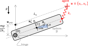
Figure 1: Inverted Pendulum

We shall consider a moving-frame $\{1\}$ attached to the $com$ of the pendulum and rotating with it by angle $\alpha$ (see Fig.1) with respect to the space-frame $\{0\}$. For convenience, we shall define the (unit-length) axis ${\boldsymbol{n}}_{\alpha}$ directed along the major axis, the (unit-length) axis ${\boldsymbol{n}}_{\alpha}^{\perp}$ perpendicular to it as well as the rotation matrix ${\boldsymbol{R}}_{\alpha}$ as follows:

$${\boldsymbol{n}}_{\alpha}=\begin{bmatrix}\cos\alpha\\ \sin\alpha\end{bmatrix}\hskip 17.07182pt{\boldsymbol{n}}_{\alpha}^{\perp}=\begin{bmatrix}-\sin\alpha\\ \cos\alpha\end{bmatrix}\hskip 17.07182pt{\boldsymbol{R}}_{\alpha}=\begin{bmatrix}\cos\alpha&-\sin\alpha\\ \sin\alpha&\cos\alpha\end{bmatrix}$$ (31)

As shown in Fig.1, the pendulum is subject gravitational potential $W_{grav}$ (due to a constant force $mg$, pointing downwards and acting at $com$) as well as to the elastic (control) potential $W_{ctrl}$ due to a linear spring of stiffness $k_{c}$ attached between an agent-controlled position ${\boldsymbol{u}}=(u_{x},u_{y})$ and the tip of the pendulum ${\boldsymbol{c}}=L_{0}{\boldsymbol{n}}_{\alpha}$. The total potential $W$ can then be expressed as

$$\begin{matrix}W(\alpha,{\boldsymbol{u}})&=&W_{grav}+W_{ctrl}\hfill\\ &=&\frac{1}{2}mgL_{0}\sin\alpha+\frac{1}{2}k_{c}\|{\boldsymbol{u}}-L_{0}{\boldsymbol{n}}_{\alpha}\|^{2}\hfill\\ &=&\frac{1}{2}mgL_{0}\sin\alpha+\frac{1}{2}k_{c}((u_{x}-L_{0}\cos\alpha)^{2}+(u_{y}-L_{0}\sin\alpha)^{2})\hfill\end{matrix}$$ (32)

4.1 Case 1: constant spring $k_{c}$

As a first case, we shall consider a linear spring of constant stiffness $k_{c}$. In this case, first and higher derivatives of the potential energy (32) become straightforward and can be tackled analytically.

4.1.1 Equilibria

For a given control input ${\boldsymbol{u}}$, the equilibrium position(s) of the pendulum can found from (9), where the variable ${\boldsymbol{z}}$ is identified with the scalar $\alpha$ (the pendulum angle) in this example

$$\begin{matrix}0&=&\nabla_{{\boldsymbol{z}}}W\hfill\\ &=&k_{c}L_{0}(u_{x}\sin\alpha-(u_{y}-mg/2k_{c})\cos\alpha)\\ &=&-k_{c}L_{0}({\boldsymbol{n}}_{\alpha}^{\perp})^{T}({\boldsymbol{u}}-{\boldsymbol{u}}_{crit})\hfill\end{matrix}$$ (33)

where ${\boldsymbol{u}}_{crit}:=[0\ mg/2k_{c}]^{T}$ denotes a critical point where the system will display instability, as it will be shown soon.

As the pendulum is a physical system in the standard Euclidean space (2D, for simplicity), what follows will be make use of the familiar Euclidean norm. It is apparent that (33) expresses an orthogonality condition between the vector ${\boldsymbol{u}}-{\boldsymbol{u}}_{crit}$ and the unit vector ${\boldsymbol{n}}_{\alpha}^{\perp}$ (which is, in turn, perpendicular to the pendulum). Therefore ${\boldsymbol{u}}-{\boldsymbol{u}}_{crit}$ is either aligned (+) or anti-aligned (-) with the pendulum direction ${\boldsymbol{n}}_{\alpha}$, i.e. (33) is equivalent to

$${\boldsymbol{u}}-{\boldsymbol{u}}_{crit}=\pm L_{u}{\boldsymbol{n}}_{\alpha}$$ (34)

where, as also shown in Fig.1, control length $L_{u}$ is defined as

$$L_{u}:=\|{\boldsymbol{u}}-{\boldsymbol{u}}_{crit}\|=\sqrt{u_{x}^{2}+(u_{y}-mg/2k_{c})^{2}}$$ (35)

Away from the critical point (i.e. ${\boldsymbol{u}}\neq{\boldsymbol{u}}_{crit}$ or, equivalently, $L_{u}>0$), analytical solutions of (33) can be described as

$${\boldsymbol{z}}_{m}^{*}({\boldsymbol{u}}):=\text{atan2}(u_{y}-mg/2k_{c},u_{x})+m\pi$$ (36)

where $m=0$ corresponds to the aligned (+) case and $m=1$ corresponds to the anti-aligned case (-). Given the periodicity of the problem, any other value of multeplicity $m$ can be considered equivalent to $m=0$ (if even) or to $m=1$ (if odd). Below, it will be shown that $m=0$ is a stable solution while $m=1$ is unstable. We shall therefore only consider the stable solution

$$\alpha^{*}:={\boldsymbol{z}}_{0}^{*}({\boldsymbol{u}})=\text{atan2}(u_{y}-mg/2k_{c},u_{x})$$ (37)

Restricting the potential to the equilibrium manifold leads to the reduced potential

$$W^{*}({\boldsymbol{u}}):=W(\alpha^{*},{\boldsymbol{u}})=\frac{1}{2}k_{c}(L_{u}-L_{0})^{2}+\frac{1}{2}mg\,u_{y}+const$$ (38)

This can be verified by noting that the stable equilibrium condition (34), i.e. the one with the positive sign, corresponds to $u_{x}=L_{u}\cos\alpha$ and $u_{y}=L_{u}\sin\alpha+mg/2l_{c}$ which, substituted back in (32), after some algebraic manipulation, lead to eq.(38).

Remark:the constant and linear terms in (38) are inessential for the purpose of evaluating the Hessian which, therefore, only depends on the quadratic term $1/2k_{c}^{2}(L_{u}-L_{0})^{2}$. Such term captures the radial push/pull, it only affects the reaction forces at the hinge, not the ones against gravity.

4.1.2 Stability

To analyze stability, we will need to evaluate higher derivatives with respect to the parameter $\alpha$. To this end, it is convenient to note the following identities

$$\frac{\partial}{\partial\alpha}{\boldsymbol{n}}_{\alpha}={\boldsymbol{n}}_{\alpha}^{\perp}\hskip 28.45274pt\frac{\partial}{\partial\alpha}{\boldsymbol{n}}_{\alpha}^{\perp}=-{\boldsymbol{n}}_{\alpha}$$ (39)

through which one immediately evaluates the Hessian

$$\begin{matrix}\nabla_{{\boldsymbol{z}}{\boldsymbol{z}}}^{2}W&=&-k_{c}L_{0}(\frac{\partial}{\partial\alpha}{\boldsymbol{n}}_{\alpha}^{\perp})^{T}({\boldsymbol{u}}-{\boldsymbol{u}}_{crit})\hfill\\ &=&+k_{c}L_{0}{\boldsymbol{n}}_{\alpha}^{T}({\boldsymbol{u}}-{\boldsymbol{u}}_{crit})\hfill\\ &=&\pm k_{c}L_{0}{\boldsymbol{n}}_{\alpha}^{T}L_{u}{\boldsymbol{n}}_{\alpha}\hfill\\ &=&\pm k_{c}L_{0}L_{u}\hfill\\ \end{matrix}$$

While $k_{c}>0$, $L_{0}>0$ are strictly positive constants, the term $L_{u}$ defined in eq.(35) is strictly positive if ${\boldsymbol{u}}\neq{\boldsymbol{u}}_{crit}$. Therefore, only the aligned (+) solution in (34) ensures stability via a strictly positive Hessian, therefore we shall only consider the non-negative case

$$\nabla_{{\boldsymbol{z}}{\boldsymbol{z}}}^{2}W=k_{c}L_{0}L_{u}$$ (40)

which is in fact positive definite as long as ${\boldsymbol{u}}\neq{\boldsymbol{u}}_{crit}$.

4.1.3 Second Derivatives

In addition to the Hessian (40), in order to evaluate the reduced Hessian ${\boldsymbol{G}}_{m}({\boldsymbol{u}})$ as in (22), the remaining second derivatives have to be evaluated. Differentiating the total potential $W$ in (32) twice with respect to ${\boldsymbol{u}}$ immediately leads to

$$\nabla_{{\boldsymbol{u}}{\boldsymbol{u}}}W=\begin{bmatrix}k_{c}&0\\ 0&k_{c}\end{bmatrix}$$ (41)

Differentiating $\nabla_{{\boldsymbol{z}}}W$ in (33) with respect to ${\boldsymbol{u}}$ returns

$$\nabla_{{\boldsymbol{z}}{\boldsymbol{u}}}W=k_{c}L_{0}\begin{bmatrix}\sin\alpha\\ -\cos\alpha\end{bmatrix}=-k_{c}L_{0}{\boldsymbol{n}}_{\alpha}^{\perp}$$ (42)

and, in general, $\nabla_{{\boldsymbol{u}}{\boldsymbol{z}}}W=\nabla_{{\boldsymbol{z}}{\boldsymbol{u}}}^{T}W$.

Therefore the matrix ${\boldsymbol{G}}({\boldsymbol{z}},{\boldsymbol{u}})$ in (23) can be rewritten as

$$\begin{matrix}{\boldsymbol{G}}(\alpha,{\boldsymbol{u}})&=&\nabla_{{\boldsymbol{u}}{\boldsymbol{u}}}W-\nabla_{{\boldsymbol{z}}{\boldsymbol{u}}}W(\nabla_{{\boldsymbol{z}}{\boldsymbol{z}}}W)^{-1}\nabla_{{\boldsymbol{u}}{\boldsymbol{z}}}W\\ &=&{\tiny\begin{bmatrix}k_{c}&0\\ 0&k_{c}\end{bmatrix}}-k_{c}\frac{L_{0}}{L_{u}}{\boldsymbol{n}}_{\alpha}^{\perp}({\boldsymbol{n}}_{\alpha}^{\perp})^{T}\\ &=&{\boldsymbol{R}}_{\alpha}{\tiny\begin{bmatrix}k_{c}&0\\ 0&k_{c}\left(1-\frac{L_{0}}{L_{u}}\right)\end{bmatrix}}{\boldsymbol{R}}_{\alpha}^{T}\end{matrix}$$ (43)

while the reduced Hessian (22) can be derived by evaluating the general Hessian at the equilibrium $\alpha^{*}$ in (37)

$${\boldsymbol{G}}_{m}({\boldsymbol{u}}):={\boldsymbol{G}}(\alpha^{*},{\boldsymbol{u}})={\boldsymbol{R}}_{\alpha^{*}}{\tiny\begin{bmatrix}k_{c}&0\\ 0&k_{c}\left(1-\frac{L_{0}}{L_{u}}\right)\end{bmatrix}}{\boldsymbol{R}}_{\alpha^{*}}^{T}$$ (44)

From this form, one can immediately verify that ${\boldsymbol{n}}_{\alpha^{*}}$ and ${\boldsymbol{n}}_{\alpha^{*}}^{\perp}$ are the two eigenvectors corresponding, respectively, to a constant and strictly positive eigenvalue $k_{c}$ and to a second eigenvalue $k_{c}(1-L_{0}/L_{u})$ which is negative when the pendulum is compressed ($L_{u}<L_{0}$), zero when $L_{u}=L_{0}$ and positive otherwise.

On the other hand, by definition, the squared-Hessian ${\boldsymbol{G}}_{m}^{2}({\boldsymbol{u}})$ ensures non-negative eigenvalues

$${\boldsymbol{G}}_{m}^{2}({\boldsymbol{u}})={\boldsymbol{R}}_{\alpha^{*}}{\tiny\begin{bmatrix}k_{c}^{2}&0\\ 0&k_{c}^{2}\left(1-\frac{L_{0}}{L_{u}}\right)^{2}\end{bmatrix}}{\boldsymbol{R}}_{\alpha^{*}}^{T}$$ (45)

Remark: the eigenvectors are unaltered by this operation while the eigenvalues are squared.

4.1.4 Optimal Control via Squared-Hessian

For the (simple) problem considered in this section, the equilibrium manifold is a ruled surface defined by (36) in the 3-parameter space $(\alpha,u_{x},u_{y})$: for every value of $\alpha$, the locus of solutions $(u_{x},u_{y})$ is a line going through ${\boldsymbol{u}}$ and ${\boldsymbol{u}}_{crit}$ (we shall always assume ${\boldsymbol{u}}\neq{\boldsymbol{u}}_{crit}$).

As previously mentioned, the equilibrium conditions (36) and (34) are equivalent but the latter allows treating $\alpha$ as an independent parameter, replacing therefore ‘$s$’, for this specific example. This is useful when considering problems such as driving the pendulum quasi-statically (i.e. through consecutive equilibria) from an initial position $\alpha_{1}=-\pi/2$ to a final up-right position $\alpha_{2}=+\pi/2$ of the pendulum. Specifically, the stable condition (+) (34) can be rewritten as

$$\left\{\begin{matrix}u_{x}(\alpha)=L_{u}(\alpha)\cos\alpha\hfill\\ u_{y}(\alpha)=L_{u}(\alpha)\sin\alpha+mg/2k_{c}\end{matrix}\right.$$ (46)

where the control length $L_{u}$ is now considered as a dependent variable. The optimal problem can now be formulated as a minimization of the action

$$J=\int_{\alpha_{1}}^{\alpha_{2}}{{\boldsymbol{u}}^{\prime}}^{T}{\boldsymbol{G}}_{m}^{2}{{\boldsymbol{u}}^{\prime}}\,d\alpha$$ (47)

with initial and final conditions

$$\left\{\begin{matrix}L_{u}(\alpha_{1})=L_{1}\\ L_{u}(\alpha_{2})=L_{2}\\ \end{matrix}\right.$$ (48)

Note: the ‘prime’ $(^{\prime})$ operator denotes differentiation with respect to $\alpha$ and, from (34), one derives

$${{\boldsymbol{u}}^{\prime}}=(L_{u}{\boldsymbol{n}}_{\alpha})^{\prime}=L_{u}^{\prime}{\boldsymbol{n}}_{\alpha}+L_{u}{\boldsymbol{n}}_{\alpha}^{\perp}$$ (49)

Using the identities ${\boldsymbol{R}}_{\alpha}^{T}{\boldsymbol{n}}_{\alpha}=[1\ 0]^{T}$ and ${\boldsymbol{R}}_{\alpha}^{T}{\boldsymbol{n}}_{\alpha}^{\perp}=[0\ 1]^{T}$, the integrand in (47) corresponds to the (‘pendulum’) Lagrangian $\mathcal{L}_{pend}$ of the optimization problem and can be expanded as

$$\begin{matrix}{{\boldsymbol{u}}^{\prime}}^{T}{\boldsymbol{G}}_{m}^{2}{{\boldsymbol{u}}^{\prime}}&=&(L_{u}^{\prime}{\boldsymbol{n}}_{\alpha}^{T}+L_{u}({\boldsymbol{n}}_{\alpha}^{\perp})^{T}){\boldsymbol{R}}_{\alpha}{\tiny\begin{bmatrix}k_{c}^{2}&0\\ 0&k_{c}^{2}\left(1-\frac{L_{0}}{L_{u}}\right)^{2}\end{bmatrix}}{\boldsymbol{R}}_{\alpha}^{T}(L_{u}^{\prime}{\boldsymbol{n}}_{\alpha}+L_{u}{\boldsymbol{n}}_{\alpha}^{\perp})\hfill\\ &=&(L_{u}^{\prime}[1\ 0]+L_{u}[0\ 1]){\tiny\begin{bmatrix}k_{c}^{2}&0\\ 0&k_{c}^{2}\left(1-\frac{L_{0}}{L_{u}}\right)^{2}\end{bmatrix}}(L_{u}^{\prime}[1\ 0]^{T}+L_{u}[0\ 1]^{T})\hfill\\ &=&k_{c}^{2}{L_{u}^{\prime}}^{2}+k_{c}^{2}L_{u}^{2}(1-\frac{L_{0}}{L_{u}})^{2}\hfill\\ &=&k_{c}^{2}\underbrace{({L_{u}^{\prime}}^{2}+L_{u}^{2}+L_{0}^{2}-2L_{0}L_{u})}_{\mathcal{L}_{pend}}\hfill\\ \end{matrix}$$ (50)

An optimal solution to minimization of the action integral (47) with Lagrangian $\mathcal{L}_{pend}$ can be found from Euler Lagrange equations

$$\left(\frac{\partial\mathcal{L}_{pend}}{\partial L_{u}^{\prime}}\right)^{\prime}-\frac{\partial\mathcal{L}_{pend}}{\partial L_{u}}=0\hskip 14.22636pt\equiv\hskip 14.22636ptL_{u}^{\prime\prime}=L_{u}-L_{0}$$ (51)

Remark: This is a second order, linear equation which does not depend on parameters such as spring stiffness $k_{c}$ or pendulum weight $mg$.

To make it independent of the pendulum length as well, we can simply consider the normalized length

$$\lambda_{u}(\alpha):=L_{u}(\alpha)/L_{0}$$ (52)

and therefore the normalized differential equation

$$\lambda_{u}^{\prime\prime}=\lambda_{u}-1$$ (53)

which has solutions

$$\lambda_{u}(\alpha)=ae^{+\alpha}+be^{-\alpha}+1$$ (54)

Considering normalized initial and final lengths $\lambda_{1}:=L_{1}/L_{0}$ and $\lambda_{2}:=L_{2}/L_{0}$, the coefficient $a$ and $b$ can be determined as

$$\begin{bmatrix}a\\ b\end{bmatrix}=\begin{bmatrix}e^{+\alpha_{1}}&e^{-\alpha_{1}}\\ e^{+\alpha_{2}}&e^{-\alpha_{2}}\end{bmatrix}^{-1}\begin{bmatrix}\lambda_{1}-1\\ \lambda_{2}-1\end{bmatrix}$$ (55)

which gives the closed-form solution:

$$\lambda_{u}(\alpha)=\begin{bmatrix}e^{+\alpha}&e^{-\alpha}\end{bmatrix}\begin{bmatrix}e^{+\alpha_{1}}&e^{-\alpha_{1}}\\ e^{+\alpha_{2}}&e^{-\alpha_{2}}\end{bmatrix}^{-1}\begin{bmatrix}\lambda_{1}-1\\ \lambda_{2}-1\end{bmatrix}+1$$ (56)

Note: the 2$\times$2 matrix is invertible iff $\alpha_{1}\neq\alpha_{2}$.

Figure 2: Optimal curves $\lambda_{u}(\alpha)$ vs. $\alpha$ (top) and control positions $u_{x}(\alpha)$ vs. $u_{y}(\alpha)$ for different values of initial and final length

4.2 Towards robotic manipulation: a numerical study

The example in Fig. 1 was devised to be simple enough to allow for exact, analytical solutions. Most of real-life scenarios, however, do not share this luxury. Specifically for robotic manipulation, one major hurdle is the non-smooth nature of mechanical contact [13] for which there exist various possible approaches. Here we would like to be able to make use of the optimal control framework derived so far, for which smoothness is essential. We therefore propose to regularize contact between two bodies (e.g. $\mathcal{B}_{1}$ and $\mathcal{B}_{2}$) via a non-linear stiffness $k_{c}$ which depends on the inter-penetration $d$, as sketched in Fig. 3.

Inter-penetration is a signed distance: if two objects are in mechanical contact, we allow for some degree of interpenetration ($d<0$) and high contact forces arise from the assumption of a high level of stiffness ($k_{max}$). On the other hand, when the two objects are not in contact ($d>0$), one would expect no forces and this is modeled via a very low level of stiffness ($k_{min}\ll k_{max}$). We then assume a steep yet smooth transition (around $d\approx 0$) as sketched in the graph in Fig. 3. Analytically, this can be modeled via smooth functions such as

$$k_{c}(d)=k_{min}+\frac{1-\tanh(d/d_{0})}{2}k_{max}$$ (57)

where $d_{0}$ is a parameter capturing the penetration depth.

Computing the inter-penetration of rigid bodies for generic shapes can be computationally expensive and is typically done via numerical methods [32]. The task is much simpler when one of the bodies can be assumed to be a point, as in the case of the agent in Fig.1, represented by a point of coordinates ${\boldsymbol{u}}=(u_{x},u_{y})$.

Figure 3: Regularization of mechanical contact: based on the penetration variable $d$, a spring of with nonlinear stiffness $k_{c}$ is designed assume high-stiffness levels ($k_{max}$) when the bodies are in contact ($d<0$) and low-stiffness levels ($k_{min}$) when not in contact $d>0$. A steep yet smooth transition occurs in an interval $[-d_{0}\ d_{0}]$.

With reference to the specific 2D problem in Fig 1, to compute the penetration $d$ by the agent, localized at given point ${\boldsymbol{u}}$, within the rigid body of the pendulum, a geometrical definition of the shape of the pendulum is required. Both in 2D as well as in 3D, a simple way to proceed analytically is to model the rigid body $\mathcal{B}$ as a super-ellipse [29], for which the pseudo-distance $d$ between agent and body $\mathcal{B}$ is simply given as

$$d:=\Delta(u_{x},u_{y})$$

where $\Delta:\mathbb{E}^{2}\to\mathbb{R}$ is the super-ellipse inside-outside function

$$\Delta:(x,y)\mapsto\left(\frac{x}{a}\right)^{2/\epsilon}+\left(\frac{y}{b}\right)^{2/\epsilon}-1$$ (58)

where $0<\epsilon<2$ define the shape of the super-ellipse ($\epsilon=1$ for an ellipse, $\epsilon<1$ for a super-ellipse as in this work), while $a$ and $b$ represent half-length and half-width of the body $\mathcal{B}$, respectively.

4.2.1 Equilibrium Manifold

The configuration space $Q$ of the agent+pendulum can be parameterized by the (scalar) rotation $z\equiv\alpha\in\mathbb{R}$ of the pendulum and the 2D position ${\boldsymbol{u}}\equiv(u_{x},u_{y})\in\mathbb{R}^{2}$ of the agent, resulting in the three-dimensional manifold:

$$Q:=S^{1}\times\mathbb{R}^{2}$$ (59)

As our analysis is local, we shall assume working in an open of $\mathbb{R}\times\mathbb{R}^{2}$.

The total potential $W$ will comprise a gravitational potential $W_{grav}$ and the (control) elastic potential $W_{ctrl}$ and will be formally similar to (32). The only difference is due to the nonlinearity of the stiffness $k_{c}$, now function of the inter-penetration $d$ which can readily be evaluated via the super-ellipse function $\Delta(\cdot)$ defined in (58). This valuation is more conveniently done in the moving frame:

$$W_{ctrl}=\frac{1}{2}k_{c}(\Delta(\tilde{{\boldsymbol{u}}}))\ \|\tilde{{\boldsymbol{u}}}-\tilde{{\boldsymbol{c}}}\|^{2}$$ (60)

where $\|\cdot\|^{2}$ is the Euclidean distance; the tilde $\tilde{\cdot}$ denotes coordinates expressed in the moving frame $\{1\}$, in which, $\tilde{{\boldsymbol{c}}}$ is a constant vector and $\tilde{{\boldsymbol{u}}}:={\boldsymbol{T}}_{1}^{-1}\circ{\boldsymbol{u}}$ .

Thanks to the smoothness of the functions (57) and (58), gradients $\nabla_{{\boldsymbol{z}}}W$, $\nabla_{{\boldsymbol{u}}}W$ as well as the second derivatives $\nabla^{2}_{{\boldsymbol{u}}{\boldsymbol{z}}}W$, $\nabla^{2}_{{\boldsymbol{z}}{\boldsymbol{u}}}W$, and the Hessian $\nabla^{2}_{{\boldsymbol{z}}}W$ can be computed analytically in symbolic form, via the MATLAB Symbolic Toolbox or any other Computer Algebra System.

Using the numerical values given in Table 1, a numerical solver (fsolve in MATLAB) was used to solve the equilibrium equation (9) for an array of inputs $u_{x}$ and $u_{y}$, each spanning across 150% of workspace ($\pm L_{0}$).

parameter	value	units	description
$L_{0}$	1	$m$	pendulum length
$W_{0}$	0.1	$m$	pendulum width
$mg$	$10$	N	weight force
$k_{min}$	$1$	N/m	stiffness
$k_{max}$	$10^{4}$	N/m	stiffness
$\epsilon$	0.1	-	super-ellipse factor

Table 1: Values used in the numerical simulations.

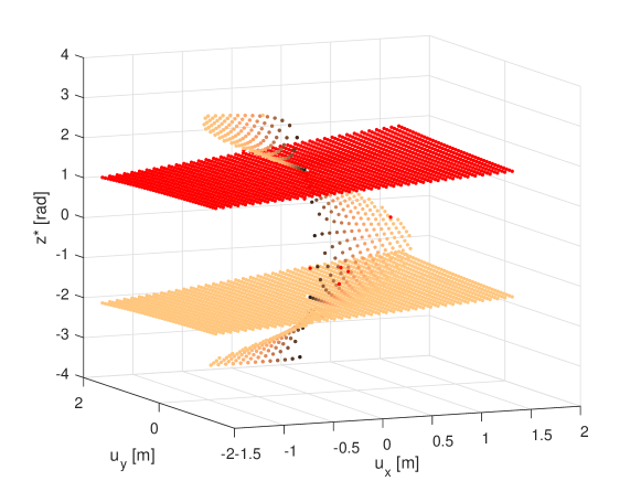
a)

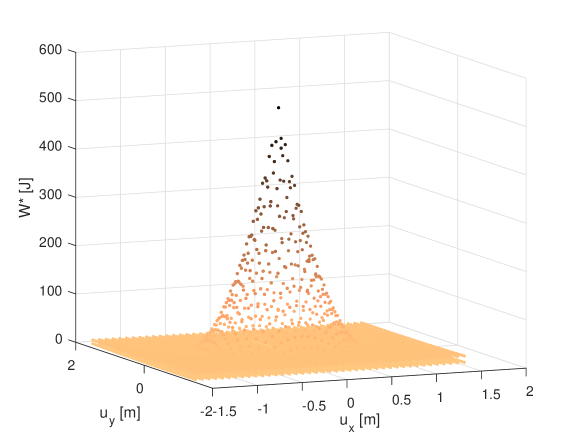
b)

Figure 4: a) Equilibrium configurations $z^{*}$ (equivalent to the rotation $\alpha$ of the pendulum) and b) equilibrium energies $W^{*}$ for an array of inputs $(u_{x},u_{y})$ spanning 150% of the workspace ($\pm L_{0}$)

At each point $(u_{x},u_{y})$ of the grid, multiple solutions $z^{*}_{m}$ (a scalar, representing an equilibrium angle $\alpha$ of the pendulum angle), each with its own with $m$ a multiplicity index were estimated by the numerical solver and are shown in Fig. 4-a), where the unstable solutions (the ‘ceiling’ at height $\alpha\approx+\pi/2$) are highlighted in red color. The remaining solutions consist of a ‘floor’ $\alpha\approx-\pi/2$ and a ‘staircase’ which is approximately the graph of eq.(36). The ‘floor’ and the ‘ceiling’ in Fig. 4-a) are only approximately horizontal due to the presence of a small but non-zero value of $k_{min}$ through which the agent still influences the pendulum at a distance ($d>0$). Figure 4-b) shows the energies relative to the same solutions, the higher energies (cone-like shape in the middle) are relative to the equilibria on the ‘staircase’. It is evident how the amount of elastic energy increases as the agent approaches the origin , due to the compression ($d\ll 0$) of the spring ($k_{c}(d)\approx k_{max}$).

4.2.2 Optimal Path on Graphs

In previous section, the the problem of optimally manipulating the pendulum in Fig. 1 was framed as an optimal path on the equilibrium manifold and solved specifically on the ‘staircase’, one of the possible branches of the equilibrium manifold, analytically defined by (36).

In real or numerical scenarios, we rarely have the luxury of an equation such as (36), locally defining a branch of the equilibrium manifold. We might just have samples of solutions, either from experiments or numerical approximations, and there might be no indication of which branch they belong to (or prior knowledge of the number of branches). In fact, the plots in Fig. 4 resemble this situation: all we have are disconnected solutions, each representing an equilibrium point in and open $\mathcal{Z}\times\mathcal{U}\in\mathbb{R}^{N\times K}$. We shall here only focus on the stable equilibria: numerically, we can always test the Hessian $\det(\nabla_{{\boldsymbol{z}}{\boldsymbol{z}}}W)$ while, experimentally, we will not be able to even witness unstable equilibria (just like we never witness a tossed coin landing and standing on its edge).

To capture the topology of the problem, we propose working on graphs. Referring to textbooks such as [19] for details, here we simply recall the following basic definition: an undirected graph is a pair $\mathcal{G}=(\mathcal{V},\mathcal{E})$ where $\mathcal{V}$ is a set of vertices and $\mathcal{E}$ is a set of edges, where each element $e_{ij}\in\mathcal{E}$ consists of an (unordered) pair of vertices $v_{i},v_{j}\in\mathcal{V}$. Two vertices are connected (i.e. ‘neighbors’ in some sense, to be specified) if there is an edge connecting them.

Figure 5: Construction of connectivity in the top-graph’ (in full configuration space $\mathbb{R}^{N}\times\mathbb{R}^{K}$) given the connectivity in the ‘bottom-graph’ (in control space $\mathbb{R}^{K}$). The sketch depicts (parts of) two branches of the EM lying ‘above’ the control point ${\boldsymbol{u}}_{j}\in\mathbb{R}^{K}$ and relative to different multiplicities (${\boldsymbol{z}}_{n_{1}}\neq{\boldsymbol{z}}_{n_{2}}$). Not shown in this figure is the fact that these two branches might actually reconnect above some set of critical points ${\boldsymbol{u}}_{c}\in\mathbb{R}^{K}$ but, for this to happen, the Hessian $\nabla_{{\boldsymbol{z}}{\boldsymbol{z}}}^{2}W$ must be rank-deficient when evaluated at $({\boldsymbol{z}}_{c},{\boldsymbol{u}}_{c})$ and condition (10) no longer holds.

With reference to Fig. 5, given the control nature of the problem, we assume that an initial graph, referred to as ‘bottom graph’ $\mathcal{G}_{bot}$, is available. In practice, this corresponds to having an array (often a regular grid) of $S$ control inputs $\{{\boldsymbol{u}}_{s}\in\mathcal{U}\}_{s=1}^{S}$. These sampling locations constitute the set of vertices for the given bottom graph $\mathcal{G}_{bot}$. With reference to the pendulum problem in Fig. 1, the inputs ${\boldsymbol{u}}_{s}$ are taken to be a regular grid of a region of the workspace and two vertices are considered connected if they are neighbors in this regular grid. Figure 5 depicts two vertices ${\boldsymbol{u}}_{i},{\boldsymbol{u}}_{j}\in\mathcal{U}$ of the bottom graph and an edge (diagonal, dashed line) connecting them. The other edges (forming parallelogram) represent connections to other neighbors and this connectivity pattern is used to tile up the whole grid.

The objective is to construct a ‘top graph’ $\mathcal{G}_{top}$ given the bottom one $\mathcal{G}_{bot}$. More specifically, given isolated solutions which constitute the vertices of $\mathcal{G}_{top}$ and which naturally project to vertices on $\mathcal{G}_{bot}$, the objective is to re-construct the connectivity on $\mathcal{G}_{top}$ based on the connectivity on $\mathcal{G}_{bot}$.

To each vertex ${\boldsymbol{u}}_{i}$ on $\mathcal{G}_{bot}$ there correspond possibly multiple vertices, denoted as $({\boldsymbol{z}}^{*}_{m},{\boldsymbol{u}}_{i})$, in $\mathcal{G}_{top}$, where $m=1,2,\dots,$ is the multiplicity of solutions of (9). Since each solution ${\boldsymbol{z}}^{*}_{m}$ is found only after the control input ${\boldsymbol{u}}_{i}$ is specified, there exists a natural projection

$$\text{pr}:({\boldsymbol{z}}^{*}_{m},{\boldsymbol{u}}_{i})\mapsto{\boldsymbol{u}}_{i}$$ (61)

Given a solution (vertex) $({\boldsymbol{z}}^{*}_{m},{\boldsymbol{u}}_{i})$ on the top graph and control ${\boldsymbol{u}}_{j}$ connected to ${\boldsymbol{u}}_{i}$ on the bottom graph, we would like to establish which of the solutions $({\boldsymbol{z}}^{*}_{n},{\boldsymbol{u}}_{j})$ projecting to ${\boldsymbol{u}}_{j}$ should be connected to $({\boldsymbol{z}}^{*}_{m},{\boldsymbol{u}}_{i})$. In other words, which of the solutions $({\boldsymbol{z}}^{*}_{n},{\boldsymbol{u}}_{j})$ lies on the same branch as $({\boldsymbol{z}}^{*}_{m},{\boldsymbol{u}}_{i})$.

Assuming a relatively dense grid, the idea is to numerically approximate a branch with a tangent space at $({\boldsymbol{z}}^{*}_{m},{\boldsymbol{u}}_{i})$. Therefore, of all possible solutions ${\boldsymbol{z}}^{*}_{n}$ projecting down on the same ${\boldsymbol{u}}_{j}$, we should consider the one for which ${\boldsymbol{z}}^{*}_{n}$ is ‘closest’ to ${\boldsymbol{z}}^{*}_{m}+\delta{\boldsymbol{z}}_{j,i,m})$ where, from eq.(15),

$$\delta{\boldsymbol{z}}_{j,i,m}=-(\nabla_{{\boldsymbol{z}}{\boldsymbol{z}}}^{2}W|_{*mi})^{-1}\nabla^{2}_{{\boldsymbol{u}}{\boldsymbol{z}}}W|_{*mi}({\boldsymbol{u}}_{j}-{\boldsymbol{u}}_{i})$$ (62)

where the notation $|_{*mi}$ denotes that the gradients are evaluated at $({\boldsymbol{z}}_{m}^{*},{\boldsymbol{u}}_{i})$.

This is sketched in Fig. 5), where the plane $\Pi$ is tangent at $({\boldsymbol{z}}^{*}_{n},{\boldsymbol{u}}_{j})$ to the $m$-th branch, according to eq.(15).

Remark [fiber-wise distance]: the reasoning above made use of the concept of ‘closeness’ between ${\boldsymbol{z}}^{*}_{n}$ and ${\boldsymbol{z}}^{*}_{m}+\delta{\boldsymbol{z}}$. This distance is evaluated on the ‘fiber’ above ${\boldsymbol{u}}_{j}$ and this distance is inherent to the mechanical configuration of the space $\mathcal{Z}\in\mathbb{R}^{N}$. We assume a fiber-wise distance, perhaps multiple ones, can always for a given problem at hand. In the specific case of the pendulum, it simply refers to difference in orientation $\alpha$ between two configurations and such a difference is evaluated modulo $2\pi$.

Once a connectivity is built on $\mathcal{G}_{top}$, each edge can be assigned a non-negative weight: if two vertices $({\boldsymbol{z}}^{*}_{n},{\boldsymbol{u}}_{j})$ and $({\boldsymbol{z}}^{*}_{m},{\boldsymbol{u}}_{i})$ of the top graph $\mathcal{G}_{top}$ are connected, a non-negative weight $w_{j,i,m}$ is defined as the squared-Hessian:

$$w_{j,i,m}:=({\boldsymbol{u}}_{j}-{\boldsymbol{u}}_{i})^{T}{\boldsymbol{G}}|_{*mi}^{2}({\boldsymbol{u}}_{j}-{\boldsymbol{u}}_{i})$$ (63)

where ${\boldsymbol{G}}|_{*mi}$ is the Hessian defined in (22) and evaluated at $({\boldsymbol{z}}_{m}^{*},{\boldsymbol{u}}_{i})$.

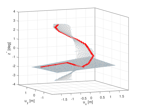
Figure 6: Minimum path over the top-graph $\mathcal{G}_{top}$ connecting two (arbitrary) points.

Standard search algorithms are available for finding optimal paths on graphs given non-negative weight connectivity. Fig. 6 shows a graph $\mathcal{G}_{top}$ obtained from numerical solutions following the procedure described above. An optimal path is highlighted connecting two points, chosen to be on different branches. One noteworthy aspect is that the the only way to go up on the ‘staircase’ (i.e. reversing the pendulum) is to pass through the intersections between ‘floor’ and ‘staircase’. In this sense, the algorithm is able to navigate a multivalued map, finding passageways in-between branches.

We believe that this might lead to a topological description of the manipulation tasks.

Appendix A Appendix - Tensorial properties of the Hessian

A.1 Standard formulas from matrix calculus

Consider the following (scalar) potential

$$f:\mathbb{R}^{n}\to\mathbb{R}$$ (64)

The Hessian at a point ${\boldsymbol{x}}\in\mathbb{R}^{n}$ is defined as

$$\nabla_{{\boldsymbol{x}}{\boldsymbol{x}}}^{2}f:=\nabla_{{\boldsymbol{x}}}\nabla_{{\boldsymbol{x}}}^{T}f$$ (65)

Consider a change of coordinates

$${\boldsymbol{x}}={\boldsymbol{X}}({\boldsymbol{\tilde{x}}})\hskip 28.45274pt\Leftrightarrow\hskip 28.45274pt\delta{\boldsymbol{x}}={\boldsymbol{J}}\delta{\boldsymbol{\tilde{x}}}$$ (66)

where ${\boldsymbol{X}}:\mathbb{R}^{n}\to\mathbb{R}^{n}$ is locally smooth and invertible, and the new scalar function and ${\boldsymbol{J}}$ its Jacobian.

In new coordinates system, the potential is defined as

$$\tilde{f}({\boldsymbol{\tilde{x}}}):=f({\boldsymbol{X}}({\boldsymbol{\tilde{x}}}))\hskip 28.45274pt\Leftrightarrow\hskip 28.45274ptd\tilde{f}=df{\boldsymbol{J}}$$ (67)

where differentials $df,d\tilde{f}$ are intended as row vectors, it follows that gradients (column vectors) and therefore forces transform as

$$\nabla_{{\boldsymbol{\tilde{x}}}}\tilde{f}={\boldsymbol{J}}^{T}\nabla_{{\boldsymbol{x}}}f$$ (68)

The Hessian in new coordinates is given as

$$\nabla^{2}_{{\boldsymbol{\tilde{x}}}{\boldsymbol{\tilde{x}}}}\tilde{f}={\boldsymbol{J}}^{T}\nabla_{{\boldsymbol{x}}{\boldsymbol{x}}}f{\boldsymbol{J}}+\underbrace{\begin{bmatrix}\frac{\partial{\boldsymbol{J}}}{\partial x_{1}^{\prime}}\nabla_{{\boldsymbol{x}}}f&\cdots&\frac{\partial{\boldsymbol{J}}}{\partial x_{n}^{\prime}}\nabla_{{\boldsymbol{x}}}f\end{bmatrix}}_{\text{non-covariant}}$$ (69)

Remark: The Hessian is covariant if the second term in(69) is null. This is guaranteed at critical points ($\nabla_{{\boldsymbol{x}}}f=0$).

Let ${\boldsymbol{K}}:=\nabla^{2}_{{\boldsymbol{x}}{\boldsymbol{x}}}f$ and ${\boldsymbol{\tilde{K}}}:=\nabla^{2}_{{\boldsymbol{\tilde{x}}}{\boldsymbol{\tilde{x}}}}\tilde{f}$ represent stiffness matrices (i.e. Hessians of some potential) in two different coordinate frames. At equilibrium, the following transformation holds

$${\boldsymbol{\tilde{K}}}={\boldsymbol{J}}^{T}{\boldsymbol{K}}{\boldsymbol{J}}$$ (70)

Suppose $\delta{\boldsymbol{x}}$ is an eigenvector of ${\boldsymbol{K}}$ with eigenvalue $\lambda$, i.e.

$${\boldsymbol{K}}\delta{\boldsymbol{x}}=\lambda\delta{\boldsymbol{x}}$$ (71)

The corresponding vector $\delta{\boldsymbol{\tilde{x}}}$ in new coordinates, i.e. $\delta{\boldsymbol{x}}={\boldsymbol{J}}\delta{\boldsymbol{\tilde{x}}}$, is an eigenvector (with same eigenvalue $\lambda$) only if the following orthonormality condition holds

$${{\boldsymbol{J}}^{-1}={\boldsymbol{J}}^{T}}$$ (72)

Proof:

$$\begin{matrix}{\boldsymbol{K}}\delta{\boldsymbol{x}}&=&\lambda\delta{\boldsymbol{x}}\\ {\boldsymbol{K}}{\boldsymbol{J}}\delta{\boldsymbol{\tilde{x}}}&=&\lambda{\boldsymbol{J}}\delta{\boldsymbol{\tilde{x}}}\\ {{\boldsymbol{J}}^{-1}}{\boldsymbol{K}}{\boldsymbol{J}}\delta{\boldsymbol{\tilde{x}}}&=&\lambda\delta{\boldsymbol{\tilde{x}}}\\ {\boldsymbol{\tilde{K}}}\delta{\boldsymbol{\tilde{x}}}&=&\lambda\delta{\boldsymbol{\tilde{x}}}\\ \end{matrix}$$ (73)

Remark: If Hessians transform covariantly (70) and the orthonormality condition (72) holds then the squared-Hessian ${\boldsymbol{K}}^{2}$ (in fact, any power) will transform covariantly

$${\boldsymbol{\tilde{K}}}^{2}=({\boldsymbol{J}}^{T}{\boldsymbol{K}}{\boldsymbol{J}})^{2}={\boldsymbol{J}}^{T}{\boldsymbol{K}}^{2}{\boldsymbol{J}}$$ (74)

Invariance for our problem

To fit our problem, consider the following renaming of variables

$${\boldsymbol{x}}\equiv[z_{1},\dots,z_{N},u_{1},\dots,u_{K}]^{T}\equiv\begin{bmatrix}{\boldsymbol{z}}\\ {\boldsymbol{u}}\end{bmatrix}$$

$$f({\boldsymbol{x}})\equiv W({\boldsymbol{z}},{\boldsymbol{u}})$$

Note that

$$\nabla_{{\boldsymbol{x}}}f=\begin{bmatrix}\nabla_{{\boldsymbol{z}}}W\\ \nabla_{{\boldsymbol{u}}}W\end{bmatrix}=\begin{bmatrix}{\boldsymbol{0}}\\ \nabla_{{\boldsymbol{u}}}W\end{bmatrix}$$

The following control-affine change of coordinates renders the non-covariant term in (69) null

$${\boldsymbol{X}}({\boldsymbol{\tilde{x}}})\equiv\begin{bmatrix}{\boldsymbol{z}}\\ {\boldsymbol{u}}\end{bmatrix}=\begin{bmatrix}{\boldsymbol{\phi}}({\boldsymbol{\tilde{z}}})+{\boldsymbol{B}}({\boldsymbol{\tilde{z}}}){\boldsymbol{\tilde{u}}}\\ {\boldsymbol{A}}({\boldsymbol{\tilde{z}}}){\boldsymbol{\tilde{u}}}\end{bmatrix}$$ (75)

Note: this leads to a Jacobian which is independent of controls ${\boldsymbol{\tilde{u}}}$, i.e.

$${\boldsymbol{J}}=\begin{bmatrix}\nabla_{{\boldsymbol{\tilde{z}}}}{\boldsymbol{\phi}}({\boldsymbol{\tilde{z}}})+\nabla_{{\boldsymbol{\tilde{z}}}}{\boldsymbol{B}}({\boldsymbol{\tilde{z}}})\\ \nabla_{{\boldsymbol{\tilde{z}}}}{\boldsymbol{A}}({\boldsymbol{\tilde{z}}})\end{bmatrix}\Longrightarrow\frac{\partial{\boldsymbol{J}}}{\partial\tilde{u}_{k}}={\boldsymbol{0}}$$

A.2 Squared-Hessian as a natural metric on the Lagrangian submanifold

In this section, we show how to construct an ‘intrinsic’ metric on the Lagrangian submanifold $\Lambda_{m}$. For the convenience of the reader, we recall that $W{{}_{m}^{*}}({\boldsymbol{u}})=W({\boldsymbol{z}}_{m}({\boldsymbol{u}}),{\boldsymbol{u}})$ and remark that $\Lambda_{m}$ is identificable ($\simeq$) by isomorphism with $\mathbb{R}^{K}$, then $\iota\simeq dW{{}_{m}^{*}}$ and $T\iota\simeq TdW{{}_{m}^{*}}$. Here, we shall also use ${\boldsymbol{f}}({\boldsymbol{u}}){=-dW_{m}^{*}}$ as a shorthand for ${\boldsymbol{f}}_{ctrl}({\boldsymbol{z}}_{m}({\boldsymbol{u}}),{\boldsymbol{u}})$ defined in (19), where ${\boldsymbol{z}}_{m}({\boldsymbol{u}})$ is a well defined function whenever the rank condition (10) is satisfied.

For $TT^{*}\mathbb{R}^{K}$ there exist the following tangent ($T_{\pi}{{}_{\mathbb{R}^{K}}}$) and vertical ($V_{\pi}{{}_{\mathbb{R}^{K}}}$) fibrations:

On the tangent and cotangent bundles the Euclidean metric is defined, respectively, as

An arbitrary curve on $\mathbb{R}\ni s\mapsto{\boldsymbol{u}}(s)\in\mathbb{R}^{K}\simeq_{\text{id}}\Lambda_{m}$, together with its generated tangent vectors, can be lifted on $T\Lambda_{m}$ as follows

By the following vertical pull-back from $T^{*}\mathbb{R}^{K}$ to $T\Lambda_{m}$ of the Euclidean metric $\mathbb{I}^{-1}$ on $T^{*}\mathbb{R}^{K}$, we are able to define the metric $\mathfrak{g}_{\Lambda_{m}}$, finally involving ${\boldsymbol{G}}_{m}^{2}$ introduced in (22):

$$\begin{matrix}\mathfrak{g}_{\Lambda_{m}}({\boldsymbol{u}})({\boldsymbol{\dot{u}}},{\boldsymbol{\dot{u}}})&:=&{\mathbb{I}}^{-1}(V_{\pi_{\mathbb{R}^{K}}}\circ T\iota({\boldsymbol{\dot{u}}}),V_{\pi_{\mathbb{R}^{K}}}\circ T\iota({\boldsymbol{\dot{u}}}))\\ &=&{\mathbb{I}}^{-1}({\boldsymbol{f}}^{\prime}({\boldsymbol{u}}){\boldsymbol{\dot{u}}},{\boldsymbol{f}}^{\prime}({\boldsymbol{u}}){\boldsymbol{\dot{u}}})\hfill\\ &=&{\mathbb{I}}^{-1}({\boldsymbol{G}}_{m}({\boldsymbol{u}}){\boldsymbol{\dot{u}}},{\boldsymbol{G}}_{m}({\boldsymbol{u}}){\boldsymbol{\dot{u}}})\hfill\\ &=&{\boldsymbol{\dot{u}}}^{T}{\boldsymbol{G}}_{m}^{2}{\boldsymbol{\dot{u}}}.\hfill\end{matrix}$$

References

- [1] Abraham, R., Marsden, J. E. (2008). Foundations of mechanics (No. 364). American Mathematical Soc..
- [2] Arnold, V. I. (1989). Mathematical methods of classical mechanics (Vol. 60). Springer Science and Business Media.
- [3] Arnold V.I., Gusein-Zade S.M., Varchenko A.N. (2012) Singularities of Differentiable Maps, Volume 1: Classification of Critical Points, Caustics and Wave Fronts (Modern Birkhäuser Classics) 2012 Edition
- [4] Atkeson C G and Hollerbach J M (1985) Kinematic features of unrestrained vertical arm movements J. Neurosci. 5 2318–30
- [5] Bazant, ZP and Cedolin, L (2010). Stability of Structures. World Scientific.
- [6] Benenti, S. (2011). Hamiltonian structures and generating families (pp. xiv+-258). New York, NY, USA: Springer.
- [7] Bressan, Alberto; Rampazzo, Franco Moving constraints as stabilizing controls in classical mechanics. Arch. Ration. Mech. Anal. 196 (2010), no. 1, 97–141.
- [8] Bressan, Alberto; Han, Ke; Rampazzo, Franco On the control of non holonomic systems by active constraints. Discrete Contin. Dyn. Syst. 33 (2013), no. 8, 3329–3353.
- [9] Bressan, Aldo On control theory and its applications to certain problems for Lagrangian systems. On hyper-impulsive motions for these. III. Strengthening of the characterizations performed in Parts I and II, for Lagrangian systems. An invariance property. Atti Accad. Naz. Lincei Rend. Cl. Sci. Fis. Mat. Nat. (8) 82 (1988), no. 3, 461–471 (1990).
- [10] Bressan, Aldo Hyper-impulsive motions and controllizable coordinates for Lagrangian systems. Atti Accad. Naz. Lincei Mem. Cl. Sci. Fis. Mat. Natur. Sez. Ia (8) 19 (1989), no. 7, 195–246 (1991).
- [11] Bressan, Aldo; Motta, Monica A class of mechanical systems with some coordinates as controls. A reduction of certain optimization problems for them. Solution methods. Atti Accad. Naz. Lincei Cl. Sci. Fis. Mat. Natur. Mem. (9) Mat. Appl. 2 (1993), no. 1, 30 pp.
- [12] Brockett, R. W., Stokes, A. (1991). On the synthesis of compliant mechanisms. In Proceedings. 1991 IEEE International Conference on Robotics and Automation (pp. 2168-2169). IEEE Computer Society..
- [13] Brogliato, B. (1999). Nonsmooth mechanics (Vol. 3). London: Springer-Verlag.
- [14] Bullo, F. and Lewis, A. D. (2005). Geometric control of mechanical systems: modeling, analysis, and design for simple mechanical control systems (Vol. 49). Springer.
- [15] Callen, H. B. (1960). Thermodynamics and an Introduction to Thermostatistics. John Wiley & Sons, New York.
- [16] Cardin, F. (2015). Elementary symplectic topology and mechanics (Vol. 16). Berlin/Heidelberg, Germany: Springer.
- [17] Cardin, Franco; Favretti, Marco Hyper-impulsive motion on manifolds. Dynam. Contin. Discrete Impuls. Systems 4 (1998), no. 1, 1–21.
- [18] Cardin, F., Zanzotto, G. (1989). On constrained mechanical systems: D’Alembert’s and Gauss’ principles. Journal of mathematical physics, 30(7), 1473-1479.
- [19] Edelsbrunner, H., Harer, J. L. (2022). Computational topology: an introduction. American Mathematical Society.
- [20] Ekeland, I. (1977). Legendre duality in nonconvex optimization and calculus of variations. SIAM Journal on Control and Optimization, 15(6), 905-934.
- [21] Gallavotti, G. (1999). Statistical mechanics: A short treatise. Springer Science & Business Media.
- [22] Gallavotti, G. (2013). Foundations of fluid dynamics. Springer Science & Business Media.
- [23] K. F. Gauss (1829) Uber ein neues allgemeines Grundgesetz der Mechanik. Crelle Journal fur die reine und angewandte Mathematik 4, 232-235 .
- [24] Gilmore, R. (1981) Catastrophe Theory for Scientists and Engineers. Wiley, New York.
- [25] Gilmore, R. (1984). Length and curvature in the geometry of thermodynamics. Physical Review A, 30(4), 1994.
- [26] Gruber, C., Brechet, S. D. (2011). Lagrange equations coupled to a thermal equation: mechanics as consequence of thermodynamics. Entropy, 13(2), 367-378.
- [27] Guigon E, Baraduc P and Desmurget M (2007) Computational motor control: redundancy and invariance J. Neurophysiol. 97 331–47.
- [28] Hollerbach J M and Flash T 1982 Dynamic interactions between limb segments during planar arm movement Biol. Cybern. 44 67–77.
- [29] Jaklic, A., Leonardis, A., Solina, F., Solina, F. (2000). Segmentation and recovery of superquadrics (Vol. 20). Springer Science & Business Media.
- [30] Kana, S., Tee, K. P., Campolo, D. (2021). Human–robot co-manipulation during surface tooling: A general framework based on impedance control, haptic rendering and discrete geometry. Robotics and Computer-Integrated Manufacturing, 67, 102033.
- [31] Kapitza, P. L. (1951). A pendulum with oscillating suspension. Uspekhi fizicheskikh nauk, 44, 7-20.
- [32] Kurtz, V., Lin, H. (2022). Contact-Implicit Trajectory Optimization with Hydroelastic Contact and iLQR. arXiv preprint arXiv:2202.13986.
- [33] Kurtzer I, DiZio P A and Lackner J R (2005) Adaptation to a novel multi-force environment Exp. Brain Res. 164 120–32.
- [34] Lilov, L., Lorer, M. (1982). Dynamic analysis of multirigid‐body system based on the Gauss principle. ZAMM‐Journal of Applied Mathematics and Mechanics/Zeitschrift für Angewandte Mathematik und Mechanik, 62(10), 539-545.
- [35] Loncaric, J. (1985). Geometrical analysis of compliant mechanisms in robotics (Euclidean group, elastic systems, generalized springs. Harvard University.
- [36] Loncaric, J. (1987). On statics of elastic systems and networks of rigid bodies. Maryland Univ College Park Systems Research Center.
- [37] Loncaric, J. (1991). Passive realization of generalized springs. In Proceedings of the 1991 IEEE International Symposium on Intelligent Control (pp. 116-121). IEEE.
- [38] Marle, Charles-Michel, Sur la géométrie des systèmes mécaniques à liaisons actives. (French. English summary) [Geometry of mechanical systems with active constraints] C. R. Acad. Sci. Paris Sér. I Math. 311 (1990), no. 12, 839–845.
- [39] Marle, Charles-Michel Géométrie des systèmes mécaniques à liaisons actives. (French) [Geometry of mechanical systems with active constraints] Symplectic geometry and mathematical physics (Aix-en-Provence, 1990), 260–287, Progr. Math., 99, Birkhäuser Boston, Boston, MA, 1991.
- [40] Salamon, P., Berry, R. S. (1983). Thermodynamic length and dissipated availability. Physical Review Letters, 51(13), 1127.
- [41] Spirkl, W., Ries, H. (1995). Optimal finite-time endoreversible processes. Physical Review E, 52(4), 3485.
- [42] Spivak, M. (2018). Calculus on manifolds: a modern approach to classical theorems of advanced calculus. CRC press.
- [43] Tommasino, P. and Campolo, D. (2017). Task-space separation principle: a force-field approach to motion planning for redundant manipulators. Bioinspiration & biomimetics, 12(2), 026003.
- [44] van der Schaft, A. (2021). Classical thermodynamics revisited: A systems and control perspective. IEEE Control Systems Magazine, 41(5), 32-60.
- [45] Zefran, M. and Bullo, F., Lagrangian Dynamics, in Kurfess, T. R. (Ed.). (2005). Robotics and automation handbook (Vol. 414). Boca Raton, FL: CRC press.