Inductive diagrams for causal reasoning

Abstract.

The Lamport diagram is a pervasive and intuitive tool for informal reasoning about causality in a concurrent system. However, traditional axiomatic formalizations of Lamport diagrams can be painful to work with in a mechanized setting like Agda, whereas inductively-defined data would enjoy structural induction and automatic normalization. We propose an alternative, inductive formalization — the causal separation diagram (CSD) — that takes inspiration from string diagrams and concurrent separation logic. CSDs enjoy a graphical syntax similar to Lamport diagrams, and can be given compositional semantics in a variety of domains. We demonstrate the utility of CSDs by applying them to logical clocks — widely-used mechanisms for reifying causal relationships as data — yielding a generic proof of Lamport’s clock condition that is parametric in a choice of clock. We instantiate this proof on Lamport’s scalar clock, on Mattern’s vector clock, and on the matrix clocks of Raynal et al. and of Wuu and Bernstein, yielding verified implementations of each. Our results and general framework are mechanized in the Agda proof assistant.

1. Introduction

Concurrent systems are famously difficult to reason about. Since concurrent actions can interleave in an arbitrary order, we cannot reason about just one sequence of actions; we must contend with a combinatorial explosion of potential linearizations. Bringing (partial) order to this chaos is causality, the principle that an effect cannot happen before its cause. In both shared-memory and message-passing systems, causality undergirds every protocol for strengthening the communication model beyond asynchrony: we commit to performing certain actions only once we have observed others, so that observers of the effects of our action will understand that we have, indeed, observed the effects of the first.

Figure 1. An assortment of Lamport diagrams from the literature. In these examples, time flows from top to bottom (Ellis and Gibbs, 1989; Weil et al., 2006; Mathur et al., 2022), from left to right (Castro and Liskov, 1999; Lesani et al., 2016), or, rarely, from bottom to top (Lamport, 1978), and parallel through-lines represent processes, threads, or spatially-separated sites, while arrows represent communication between them.

A ubiquitous device for visualizing causal relationships over space and time is the Lamport diagram. Figure 1 shows diverse examples of Lamport diagrams spanning six decades of computing literature. In a Lamport diagram, agents (or “processes”) evolve over time along straight through-lines, and messages travel laterally between them. Importantly, causal relationships are reduced to simple geometric paths: two points in space and time are causally ordered if, and only if, they are connected by a forward path along the diagram.

As illustrations, Lamport diagrams are by nature informal. To support formal reasoning about concurrent systems, we need formal models that capture the same scenarios displayed by these diagrams. Lamport (1978)’s own model of executions consists of a set of processes, each with a sequence of local actions, together with a set of pairs of actions indicating send/receive communications between processes. From this data, Lamport’s causal happens-before relation can be derived, capturing all causally-related points in the execution. A similar model has arisen in the context of message sequence charts (MSCs), a more expressive cousin of the Lamport diagram (Alur et al., 2000; Ladkin and Leue, 1993; Broy, 2005; ITU-T, 2011). Because Lamport’s executions and MSCs are so similar (indeed, equivalent in their current formulations), we will refer to both of them simply as formal executions (or just executions).

Formal executions provide a strong mathematical basis for reasoning about causality in concurrent systems. However, they are typically characterized axiomatically rather than inductively. While this makes them well-suited to traditional mathematical proofs, our experience has been that applying them to mechanized proof is a considerable struggle. Proof assistants founded on constructive type theory, such as our choice of Agda, excel at problems leveraging inductive data; and some of the most powerful tools in the canon of programming language theory, including the pervasive dichotomy of syntax and semantics, are founded on inductive definitions. Ideally, then, we want to inductively factor a concurrent system into smaller pieces for local analyses, then build them back up into a global analysis. However, the collections of sets in a formal execution do not lend themselves easily to factorization without making arbitrary choices: to split an execution into a “before” and an “after”, we must make a particular choice of consistent cut through the execution. While executions can be (and certainly have been) mechanized axiomatically, we would prefer to play better to the strengths of our tools.

To that end, we return to the Lamport diagram to derive a different kind of formal execution: a causal separation diagram (or CSD). CSDs enjoy an inductive definition, built up from a small set of primitive features (emission and reception of messages, together with local actions) together with syntactic operators for sequential and concurrent composition. CSDs then constitute a syntax for describing executions of a concurrent system; and like any syntax, we can interpret CSDs into a variety of semantics. We take inspiration from concurrent separation logic in modeling the concurrent composition of actions over distributed state, and from the method of string diagrams in monoidal category theory for describing formal objects using a two-dimensional, graphical syntax. However, no familiarity with either discipline is required to read this paper.

We recover a proof-relevant analogue of Lamport’s happens-before relation by interpreting the syntax of CSDs into a semantic domain of causal paths. A causal path describes a particular potential flow of information from one point in a diagram to another: where a Lamport diagram makes causal relationships visible to the eye via geometric paths, we capture those paths directly as data. The proposition that “$e_{1}$ happens before $e_{2}$” then becomes a type $e_{1}\rightsquigarrow e_{2}$, and the terms that inhabit this type are particular paths witnessing that relationship. Because paths are also defined inductively, they become much more useful than mere truth values for further proofs.

As an in-depth case study of the application of CSDs, we consider the verification of logical clocks, a common class of devices for reifying causal information into a system at runtime. A logical clock associates some metadata (a “timestamp”) with every event, with the condition (Lamport (1978)’s “clock condition”) that whenever two events are causally ordered, their timestamps are ordered likewise. The contents of a timestamp will vary with the choice of clock; some clocks reify more causal information than others. For instance, Lamport’s original scalar clock (Lamport, 1978) flattens the partial order of events into the total order of integers, while vector clocks (Mattern, 1989; Fidge, 1988) and matrix clocks (Wuu and Bernstein, 1984; Raynal et al., 1991) yield (predictably) vector and matrix timestamps, which provide progressively higher-fidelity information.

Existing proofs of the clock condition — including mechanized proofs (Mansky et al., 2017) — apply only to individual clocks. Other work on mechanized verification of distributed systems that use logical clocks typically focuses on higher-level properties, such as causal consistency of distributed databases (Lesani et al., 2016; Gondelman et al., 2021), convergence of replicated data structures (Nieto et al., 2022), or causal order of message delivery (Nieto et al., 2022; Redmond et al., 2023). Those mechanized proofs take the clock condition as an axiom (either explicitly or implicitly) on the way to proving those higher-level properties. We address this situation by giving a generic mechanized proof of the clock condition for any realizable clock that can be realized by a system of runtime replicas — in other words, a clock defined in terms of standard “increment” and “merge” functions. Realizable clocks include the well-known scalar, vector, and matrix clocks, which we instantiate within our framework to yield a proof of the clock condition for each, in a handful of lines of Agda code. Notably, while the clock condition has previously been proved for the matrix clocks of Raynal et al. (1991) and of Wuu and Bernstein (1984), we give what appear to be the first mechanized proofs for these clocks.

In summary, the main contributions of this paper are as follows:

• Causal separation diagrams (CSDs). After presenting informal intuitions in Section 2, we describe a new formal diagrammatic language for reasoning about executions of concurrent systems (Section 3). CSDs are inspired by Lamport diagrams — a well-established visual language for expressing the behavior of distributed systems — but they are inductively defined, which makes them amenable to interpretation into many semantic domains.

• Interpreting CSDs. We present interpretations of CSDs into three semantic domains:

  • Into types: We provide an interpretation of CSDs into the domain of causal paths (Section 4). Causal paths are a proof-relevant analogue of Lamport’s happens-before relation, where any given path inductively describes a particular flow of information.

  • Into functions: We provide an interpretation of CSDs into a domain of clocks; that is, functions that compute a logical timestamp at every event (Section 5). Our interpretation is parametric in the particular choice of logical clock, so long as it is realizable as a local data structure with increment and merge operations (Section 5.1).

  • Into proofs relating types and functions: We relate the above interpretations via a third interpretation of CSDs into proofs that clocks respect causality (Section 6). This yields a proof of Lamport’s clock condition for any realizable clock whose timestamps increase with successive operations.

• Applying CSDs: verified logical clocks. Finally, we instantiate our interpretations on the clocks of Lamport, Mattern, Raynal et al., and Wuu and Bernstein, yielding mechanically verified implementations of each (Section 7). In particular, we give the first (to our knowledge) mechanized proofs of the clock condition for both matrix clocks.

All of our contributions are mechanized in the Agda proof assistant; moreover, we have published an open-source library for working with CSDs, available at github.com/lsd-ucsc/csds.

2. Deriving a new formal model of executions

In this section we recall the construction and properties of the existing model of formal executions, then manufacture a “just-so” story for their derivation from Lamport diagrams. By changing one essential step in this story, we are led to a derivation of our proposed model, the causal separation diagram (CSD).

Definition 2.1 (Formal executions (Lamport, 1978; Alur et al., 2000)).

A formal execution is:

• A set $P$ of processes, each of which is a sequence of atoms called actions; together with

• A set $M$ of messages, each of which is an ordered pair of actions across two processes (the message’s associated “send” and “receive” actions).

Definition 2.2 (Happens-before (Lamport, 1978)).

Given a formal execution, the happens-before relation on actions, written $a_{1}\leq a_{2}$, is the reflexive-transitive closure of the execution’s set of messages together with the total orders given by each process.

By tradition, we exclude from consideration executions for which happens-before fails to be antisymmetric, as these indicate a failure of causality.

The data of a formal execution can be visualized in a Lamport diagram, an informal graphical representation in which process histories become parallel lines; the actions on each history become dots along those lines; and the messages between them become arrows crossing laterally between parallel process lines. Importantly, the happens-before relation can be inferred directly from a Lamport diagram: we have $a_{i}\leq a_{j}$ if and only if there exists a forward path along the diagram from $a_{i}$ to $a_{j}$.

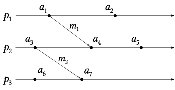
Figure 2. An example Lamport diagram.

For example, the Lamport diagram in Figure 2 depicts an execution involving three processes, $p_{1}$, $p_{2}$, and $p_{3}$, each having performed a few actions. Some of the actions in this execution are causally ordered. For instance, we see that $a_{1}\leq a_{4}$ since $a_{1}$ and $a_{4}$ are the send and receive actions of message $m_{1}$, and $a_{4}\leq a_{5}$ because they occur in sequence on $p_{2}$. Therefore, by transitivity, $a_{1}\leq a_{5}$. We also have that $a_{3}\leq a_{4}$ and $a_{3}\leq a_{7}$, among other relationships. However, $a_{1}$ and $a_{3}$ are not related by happens-before, nor are $a_{4}$ and $a_{7}$. Such pairs of actions are said to be concurrent or causally independent.

We can also take an informal diagram and formalize the scenario it displays as a formal execution. Therefore, we can consider the diagram to come first, with the derivation of an execution from an informal diagram serving as an origin story for the formal model itself. We can rederive the traditional execution by first splitting a diagram along spatial boundaries — separating the process lines from one another — and then separating the sequential actions along each process line by temporal boundaries. Doing so for the diagram in Figure 2 yields the decomposition in Figure 3(a). However, we could also have begun by laying down a sequence of temporal boundaries — demarcating global steps over the entire system — and only then separating the atomic steps within each global step by spatial boundaries. This yields the decomposition in Figure 3(b).

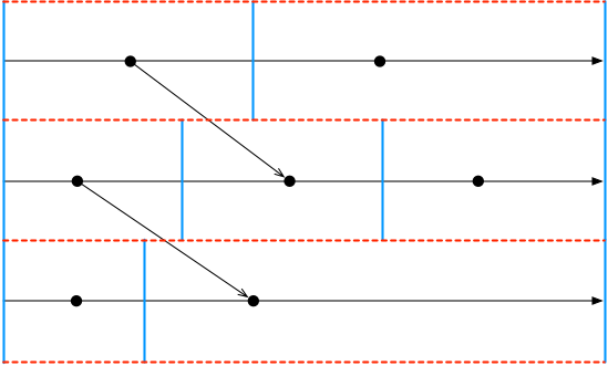
(a)   (b)

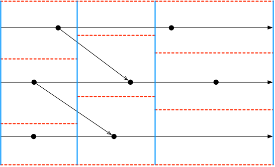
Figure 3. Two ways to decompose the Lamport diagram of Figure 2 into “tiles”. On the left (a), we split first along spatial boundaries (dashed red lines), yielding individual processes, and then along temporal boundaries (solid blue lines). On the right (b), we split first along temporal boundaries, yielding consistent cuts, and then along spatial boundaries.

Both decompositions yield a partition of the diagram into graphical tiles; and it is precisely the relationships between these tiles, witnessed by the dataflow lines passing between them, which must be captured formally. In the traditional decomposition in Figure 3(a), tiles may be related across both temporal and spatial boundaries. Process orders record the relationships across temporal boundaries, while messages record relationships across spatial boundaries. This data, comprising a traditional formal execution, is sufficient to capture all information presented in the diagram.

The state of affairs for our alternative decomposition in Figure 3(b) is notably different. First, information flows between tiles only at temporal boundaries; spatial boundaries only separate causally-independent actions which cannot influence each other. Intuitively, it takes time to move through space – spatial boundaries separate actions which may as well occur simultaneously, so the propagation of information from one place to another can only occur across temporal boundaries. However, this also means that differing quantities of state can leave a global step than enter it: a process may consume a message to decrease the quantity of data floating around, or emit a message to increase the quantity of data. Without bracing ourselves against the suggestive global geometry of fixed parallel lines for each process, we cannot even distinguish process state from message state: a global step simply transforms one configuration of separated state into another. Because of this indistinguishability, instead of referring to “processes” and “messages” we will refer only to sites: a site is a place where state exists, encompassing both processes and messages.

Second, we could have drawn different temporal boundaries — different consistent cuts — and found a different decomposition. Consistent cuts (Mattern, 1989; Chandy and Lamport, 1985) are of fundamental importance to the analysis of concurrent systems, as they model the realizable global states of a system. Thus, the formal representation for a diagram will embed a choice of consistent cuts; and as we will find in Sections 5 and 6, working with global information from the start enables simpler proof methods for reasoning about concurrent systems.

Process lines can be recovered as chosen paths spanning the diagram — that is, a chosen total order of actions, just as in the traditional execution. These path essentially names pieces of state as they evolves over time; any state not on some path is, morally, a message. We can even interpret this in a shared-memory setting: the configuration of sites along a consistent cut describe a shared heap, with each individual site modeling an exclusive region of memory. A global step then updates the heap, claiming regions by merging them and releasing regions by splitting them apart.

Figure 4 illustrates this notion of sites in more detail for our example. The shaded global step on the left has three incoming sites and five outgoing sites, so we might compactly say it has type $3\rightrightarrows 5$ (“three to five”). The next two global steps have types $5\rightrightarrows 3$ and $3\rightrightarrows 3$, respectively. Adjacent global steps must “match up” the sites on their incident site configurations; but during a global step, sites may be joined with or forked from others.

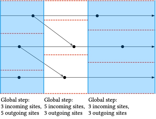
Figure 4. Global steps in our example diagram.

In Section 3, we will describe a novel formal model for concurrent executions based on these observations. However, we can already see the shape this formalization must take:

• Since we have essentially transposed the sequential and concurrent boundaries compared to the traditional formalization, our formal data will consist of a sequence of global steps acting over separated state.

• Each global step will decompose into a collection of concurrent, atomic steps, no two of which act over the same site — data flowing into and out of a global step must flow through precisely one of its constituent atomic steps. These steps include individual local actions $a_{1}$, but also include fork actions (which split one site into two) and join actions (which fuse two sites into one).

• A causal relationship between actions $a_{1}\leq a_{2}$ will be witnessed by a sequence (or path) of atomic steps, running forward from $a_{1}$ to $a_{2}$, such that adjacent steps share a site.

Our unification of messages and processes into sites makes our formalization “natively” suited for reasoning about shared-memory concurrent systems as well as distributed systems. While Lamport diagrams can effectively visualize shared-memory systems as well as distributed ones, Lamport’s formal executions are not well suited for the shared-memory domain, since processes and messages are often not the right abstractions. With CSDs, we have a diagrammatic syntax and a formal model that fit both domains.

3. Syntax and semantics of causal separation diagrams

In Section 2 we discussed the intuitions behind causal separation diagrams (CSDs), and how they arise from Lamport diagrams. In this section we give a formal treatment of CSDs as terms of an inductive data type, and develop a concept of semantic interpretations of CSDs that we will make heavy use of in later sections.

3.1. Site configurations

Recall from Section 2 that Lamport diagrams can be decomposed into a sequence of global steps, where each adjacent pair of steps meets at a collection of sites called a site configuration (or just configuration). The configuration at the start of a global step describes the state of the sites before that step takes place, while the configuration at the end describes the state of the sites after the step. The diagram as a whole also starts and ends on a pair of configurations — namely, the starting configuration of its first step, and the ending configuration of its last step. A formally-defined CSD will have type $\Gamma_{1}\rightrightarrows\Gamma_{2}$, where $\Gamma_{1}$ and $\Gamma_{2}$ are bounding configurations — the configurations the diagram begins and ends on, respectively. Site configurations are themselves terms, so $\Gamma_{1}\rightrightarrows\Gamma_{2}$ will be a dependent type. (In fact, nearly every type we define will be dependent.)

Definition 3.1 (Site configurations).

Let $\tau$ be a universe of types with products. Then a site configuration $\Gamma$ is a binary tree with leaves drawn from $\tau$, i.e., a term of the following grammar:

$$\Gamma \coloneqq\Gamma\otimes\Gamma \;\mid\;[\tau]$$

$$\tau \coloneqq\tau\times\tau \;\mid\;\dots$$

The leaf constructor $[-]$ gives the type of some state that is isolated at one site, while the spatial product $\otimes$ models a kind of separating conjunction, giving the type of state that is spatially distributed over multiple sites. For instance, if the type universe $\tau$ includes naturals $\mathbb{N}$ and booleans $\mathbb{B}$, then $[\mathbb{N}\times\mathbb{B}]\otimes[\mathbb{B}]$ is a configuration with two sites, one carrying a pair of a natural and a boolean, and the other carrying a single boolean.

The spatial product $\otimes$ is like a “lifted” version of the local product $\times$; and like the local product, we will wish to treat $\otimes$ as associative and commutative. Since reordered/rebalanced binary trees are syntactically distinct terms, however, we introduce a type of permutations $\sigma:\Gamma_{1}\simeq\Gamma_{2}$ to mediate between equivalent configurations.

Definition 3.2 (Sites).

The type $\mathrm{Site}(\Gamma)$, defined recursively over the structure of configuration $\Gamma$, is the type of paths from the root of $\Gamma$ to each of its leaves:

$$\mathrm{Site}([\tau]) =\top$$

$$\mathrm{Site}(\Gamma_{1}\otimes\Gamma_{2}) =\mathrm{Site}(\Gamma_{1})+\mathrm{Site}(\Gamma_{2})$$

Definition 3.3 (Permutations of sites ($\simeq$)).

The type of permutations $\Gamma_{1}\simeq\Gamma_{2}$ is an equivalence relation on site configurations, defined so that its elements $\sigma$ correspond to type-preserving bijections $\mathrm{Site}(\Gamma_{1})\rightarrow\mathrm{Site}(\Gamma_{2})$. By abuse of notation, we denote by $\sigma$ (and $\sigma^{-1}$) the bijection witnessed by $\sigma$.

In Definition 3.2, $\top$ is the unit type (with single value $\bullet$), and $+$ gives sum types (with injections $\mathbf{inj}_{\ell}$ and $\mathbf{inj}_{r}$). For example, the type of sites for $([\mathbb{N}]\otimes[\mathbb{B}])\otimes[\mathbb{B}]$ is $(\top+\top)+\top$. To address the site of type $\mathbb{N}$, we write the term $\mathbf{inj}_{\ell}(\mathbf{inj}_{\ell}(\bullet))$, which tells us we can isolate this site by focusing along the left-hand subtrees of this configuration.

3.2. Causal separation diagrams

From Section 2, we know that CSDs have two forms of composition: sequential composition and concurrent composition. Just as conjunctive normal form makes Boolean formulae easier to work with, we will restrict concurrent composition to appear only under sequential composition. Every CSD, then, has two layers: an outer list modeling sequencing, and an inner tree modeling concurrency. To separate these layers, we give them distinct symbols: a diagram $x:\Gamma_{1}\rightrightarrows\Gamma_{2}$ is a diagram proper, and can be composed sequentially, while a diagram $x:\Gamma_{1}\multimap\Gamma_{2}$ is a global step, and can be composed concurrently. These are morally both diagrams — a global step is just a diagram in the process of being built — and we will generally not distinguish between them.

Definition 3.4 (Causal separation diagrams ($\rightrightarrows$)).

A causal separation diagram is a sequence of global steps (see Definition 3.5, next), constructed according to the following rules:

              $\mathbf{id}:\Gamma\rightrightarrows\Gamma$      $x:\Gamma_{1}\rightrightarrows\Gamma_{2}$         $y:\Gamma_{2}\multimap\Gamma_{3}$             $(x\mathop{;}y):\Gamma_{1}\rightrightarrows\Gamma_{3}$

The id and sequencing (;) constructors play the same roles, respectively, as “nil” and “cons” do for inductive lists. We take our sequences to grow to the right (a “snoc” list) from an initial id seed, and moreover require that adjacent global steps be compatible: if a step ends on one configuration, the following step must begin on the same configuration.

Definition 3.5 (Global steps ($\multimap$)).

A global step is a binary tree of atomic steps, constructed according to the rules below:

  $x:\Gamma_{1}\multimap\Gamma_{2}$         $y:\Gamma_{1}^{\prime}\multimap\Gamma_{2}^{\prime}$      $(x\parallel y):\Gamma_{1}\otimes\Gamma_{1}^{\prime}\multimap\Gamma_{2}\otimes\Gamma_{2}^{\prime}$                        $\mathbf{fork}:[\tau\times\tau^{\prime}]\multimap[\tau]\otimes[\tau^{\prime}]$

       $\sigma:\Gamma_{1}\simeq\Gamma_{2}$     $\mathbf{perm}\ \sigma:\Gamma_{1}\multimap\Gamma_{2}$                  $\mathbf{tick}:[\tau_{1}]\multimap[\tau_{2}]$                       $\mathbf{join}:[\tau]\otimes[\tau^{\prime}]\multimap[\tau\times\tau^{\prime}]$

The atomic steps $\mathbf{tick}$, $\mathbf{fork}$, $\mathbf{join}$, and $\mathbf{perm}$ describe the elementary ways in which sites can be transformed over time. The concurrence ($\parallel$) operator fuses two global steps into one. Since the two steps must operate over distinct configurations, no atomic step can share a site with any concurrent step. Thus, just as $\otimes$ acts like a separating conjunction, $\parallel$ acts like the concurrency rule of concurrent separation logic. (We discuss future work following this analogy in Section 9.)

The perm constructor transforms a configuration into any equivalent configuration according to the type of permutations $\simeq$ of Definition 3.3. It will be convenient to have shorthand for three special cases of perm:

• $\mathbf{noop}:\Gamma\multimap\Gamma$ is a step over the identity permutation;

• $\mathbf{swap}:[\tau]\otimes[\tau^{\prime}]\multimap[\tau^{\prime}]\otimes[\tau]$ is a step commuting two sites; and

• $\mathbf{assoc}:\Gamma_{1}\otimes(\Gamma_{2}\otimes\Gamma_{3})\multimap(\Gamma_{1}\otimes\Gamma_{2})\otimes\Gamma_{3}$ is a step reassociating a configuration.

The tick constructor models any arbitrary local transformation of state. For instance, a $\mathbf{tick}$ of type $[\mathbb{N}]\multimap[\mathbb{N}\times\mathbb{B}]$ might describe an action which prepares a (boolean) message depending on the current (numeric) state. We deliberately leave the local transformations unconstrained to avoid parameterizing CSDs over yet another type. Concrete information about each individual $\mathbf{tick}$ can instead be associated to a CSD by way of labeling, which we will discuss in Section 3.3.

The fork and join constructors reify the connection between spatial and local products alluded to in Section 3.1. If we have a local pair of state at one site — for instance, a pair $[\mathbb{N}\times\mathbb{B}]$ of numeric state and prepared message — we can spatially separate its components onto two sites with fork. Conversely, state distributed over two sites can be fused into a local product on one site with join. Therefore, these steps are our analogues of the send/receive actions found in Lamport executions.

Although a traditional Lamport diagram treats send and receive actions as state-modifying actions, we factor them into two separate steps: a Lamport-style send is realized as a tick followed by a fork, and a Lamport-style receive is realized as a join followed by a tick. This factorization allows us to treat all modifications of local state uniformly via $\mathbf{tick}$, which helps us greatly when associating concrete operations to each $\mathbf{tick}$ (Section 3.3).

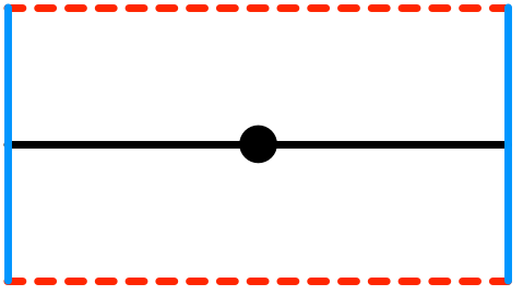
tick

fork

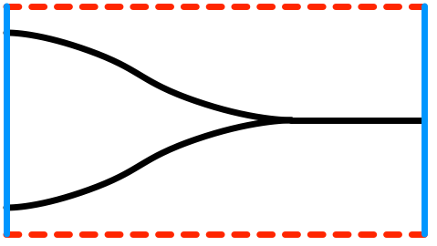
join

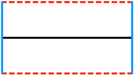
noop

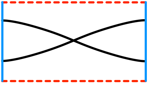
swap

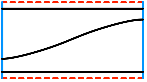
assoc

Figure 5. Atomic steps of a CSD, depicted as graphical tiles. The $\mathbf{noop}$, $\mathbf{swap}$, and $\mathbf{assoc}$ tiles characterize the more general $\mathbf{perm}$ atomic step.

Figure 5 depicts the tick, fork, join, noop, swap, and assoc atomic steps graphically. These tiles can be freely composed along like boundaries (that is, solid blue lines compose with solid blue lines, and dashed red lines compose with dashed red lines) to construct whole diagrams, so long as any sequenced pair of diagrams agree on the arrangement of sites crossing between them. For instance, consider the CSD given by the term $\mathbf{id}\mathbin{;}(\mathbf{tick}\parallel\mathbf{fork})\mathbin{;}\mathbf{assoc}\mathbin{;}(\mathbf{join}\parallel\mathbf{noop})$. As a (snoc)-list, this CSD begins from an empty diagram ($\mathbf{id}$) to which successive global steps are appended (with $\mathbin{;}$). Each constituent global step is built up as a concurrent composition of atomic steps (with $\parallel$). We can better display the structure of this CSD diagrammatically:

We begin on some site configuration $[\tau_{1}]\otimes[\tau_{2}\times\tau_{3}]$, and perform a tick on the first site and a fork on the second site to reach configuration $[\tau^{\prime}_{1}]\otimes([\tau_{2}]\otimes[\tau_{3}])$, where $\tau^{\prime}_{1}$ is the result type of the tick. With assoc, we then rebalance the configuration into $([\tau^{\prime}_{1}]\otimes[\tau_{2}])\otimes[\tau_{3}]$, so that the following step can join the first two sites (while leaving the third alone with noop). This CSD thus ends on configuration $[\tau^{\prime}_{1}\times\tau_{2}]\otimes[\tau_{3}]$. Since the type $\tau_{2}$ ends up migrating from one site to another, this CSD might describe a message sent from one process to another.

Abuses of notation

Since CSDs are lists of global steps, we can define a version of concurrent composition that acts over entire CSDs by zipping them together (with noop padding if their lengths are mismatched) and composing each pair. Likewise, we can sequentially extend a CSD by another CSD using the equivalent of a concat operator. Rather than allocate new symbols to these binary operators, we will abuse notation, letting $\parallel$ and $\mathbin{;}$ stand in for them.

In our Agda mechanization, the indexed types $\rightrightarrows$ and $\multimap$ are unified in a type with an auxiliary index over $\{\mathrm{Seq},\mathrm{Par}\}$. Throughout the rest of this paper, we take advantage of this technical contrivance to define single functions that can pattern-match through both sequential and concurrent layers of a CSD, instead of defining a separate function for each layer.

3.3. Labeled CSDs

Recall that a tick step is meant to model a local transformation of state. However, up to this point, there is no way to specify what that local transformation actually is for each tick. If we only have one transformation in a given setting, we can interpret each tick as that specific transformation. But this is clearly too much of a limitation — most systems can do more than one thing!

While we could parameterize CSDs over a type of actions (and construct each tick with a choice of action), this would complicate the type signature of CSDs, and introduce data for which the CSD itself is simply a carrier. Instead, we follow the pattern of container types (Altenkirch and Morris, 2009), in which the places where data can be held are characterized separately from the assignment of data to those places. For example, the generic type of lists $\mathrm{List}(T)$ can be factored into two parts: a Peano natural $n:\mathbb{N}$ and an assignment $\mathrm{Fin}(n)\rightarrow T$ of values to indices. The Peano natural $n$ describes a particular shape of list (with zero playing the role of the empty list, and the successor constructor playing the role of list consing), while $\mathrm{Fin}(n)$ characterizes the positions within a list of that shape. The assignment $\mathrm{Fin}(n)\rightarrow T$ then fills those positions with concrete values.

Definition 3.6 (The type of ticks).

For a CSD $X$, the type $\mathrm{Tick}(X)$ has precisely one value for every tick in $X$, and is defined recursively over the structure of $X$:

$$\mathrm{Tick}(\mathbf{tick}) =\top$$

$$\mathrm{Tick}(\mathbf{fork}) =\bot$$

$$\mathrm{Tick}(\mathbf{join}) =\bot$$

$$\mathrm{Tick}(\mathbf{perm}\ \sigma) =\bot \mathrm{Tick}(\mathbf{id}) =\bot$$

$$\mathrm{Tick}(x\parallel y) =\mathrm{Tick}(x)+\mathrm{Tick}(y) \mathrm{Tick}(x\mathbin{;}y) =\mathrm{Tick}(x)+\mathrm{Tick}(y)$$

Here, $\bot$ is the empty type, $\top$ is the unit type (with only value $\bullet$), and $+$ gives sum types (with injections $\mathbf{inj}_{\ell}$, $\mathbf{inj}_{r}$).

Definition 3.7 (Labeled CSDs).

A $T$-labeling $f:\mathrm{Tick}(X)\rightarrow T$ assigns a value of type $T$ to every tick in $X$. A $T$-labeled CSD, written $\langle X,f\rangle:\Gamma_{1}\rightrightarrows^{T}\Gamma_{2}$, is a diagram together with a $T$-labeling.

Given a labeled CSD, we can restrict its labeling to a subdiagram by pre-composing with the left or right injection for sums. For instance, the prefix of the labeled CSD $\langle(x\mathbin{;}y),f\rangle$ can be obtained as $\langle x,f\circ\mathbf{inj}_{\ell}\rangle$. In the base case, we end up with $\langle\mathbf{tick},\bullet\mapsto v\rangle$ — precisely a tick annotated with a value. This makes labeled CSDs an excellent solution for specifying the behavior of each tick.

In a traditional execution (Definition 2.1), every local action comes with some information built in — not what the action is, but who performed it. This is because every action occurs on a particular process’s total order. Although CSDs do not treat process lines specially, we can include this same information by positing a type $\mathrm{Pid}$ of process identifiers, and working in terms of $\mathrm{Pid}$-labeled CSDs.

3.4. Semantic interpretations of CSDs

The construction of the $\mathrm{Tick}$ type in Definition 3.6 is our first example of an interpretation of CSDs: we assigned some type to each atomic step, and described how sequential and concurrent composition act over those types to yield a type for larger diagrams. This pattern is emblematic of denotational semantics: “the meaning of the composition is the composition of the meanings.” By itself, the CSD representation is not much use; its utility comes from its interpretability.

Definition 3.8 (Semantic interpretations).

A semantic interpretation (or semantics, or interpretation) of CSDs is a function $(\Gamma_{1}\rightrightarrows\Gamma_{2})\rightarrow F(\Gamma_{1},\Gamma_{2})$ mapping each CSD to a semantic domain $F$ indexed by site configurations.

In the case of $\mathrm{Tick}$, we take $F(-,-)$ to be $\mathbf{Type}$, so its semantic domain does not vary with the particular bounding configurations. Much of the rest of this paper will be devoted to the construction and analysis of additional interpretations, following the landmarks given in the introduction:

• In Section 4, we give a semantics in $F(\Gamma_{1},\Gamma_{2})=\mathrm{Site}(\Gamma_{1})\rightarrow\mathrm{Site}(\Gamma_{2})\rightarrow\mathbf{Type}$, a domain of types $\rightsquigarrow$ whose elements $p_{12}:s_{1}\rightsquigarrow s_{2}$ are causal paths between sites at the boundaries of the diagram. This yields a proof-relevant analogue of Lamport’s happens-before relation, where a path gives concrete evidence for why its endpoints are causally related.

• In Section 5, we give a semantics in $F(\Gamma_{1},\Gamma_{2})=\mathrm{Valuation}(\Gamma_{1})\rightarrow\mathrm{Valuation}(\Gamma_{2})$, a domain of functions $\mathcal{C}$, parametric in a choice of logical clock. A valuation $\nu:\mathrm{Valuation}(\Gamma_{1})$ is an assignment $\mathrm{Site}(\Gamma_{1})\rightarrow\mathrm{Time}$ of timestamps to each site; so functions $\mathcal{C}$ compute timestamps $\mathcal{C}_{\nu}$ on $\Gamma_{2}$ from timestamps $\nu$ on $\Gamma_{1}$.

• In Section 6, we give a semantics in $F(\Gamma_{1},\Gamma_{2})=\forall s_{1}\ s_{2}.\ (s_{1}\rightsquigarrow s_{2})\rightarrow(\forall\nu.\ \nu(s_{1})\leq\mathcal{C}_{\nu}(s_{2}))$, a domain of proofs relating the first two interpretations via Lamport’s clock condition. The resulting proof is constructed modularly, by composing proofs over atomic steps into proofs over whole diagrams, and is parametric in a choice of logical clock.

Our target domains (happens-before, logical clocks, and the clock condition) are all pre-existing concepts in the literature. However, the interpretations sketched above only directly relate points on the beginning and ending boundaries of a diagram, while these concepts traditionally speak of points interior to a diagram. To bridge this gap, we provide a general, two-phase recipe for building interpretations.

• First we define a “spanning” interpretation, restricting the target domain to relationships between the initial and final sites of a CSD. These interpretations are typically easy to implement recursively over the structure of a CSD. For the causal paths of Section 4, this will yield a domain of “spanning paths” giving causal relationships only between the sites on the boundary of a diagram.

• Next we define an “interior” interpretation, extending the first interpretation to include relationships between points on the interior of a diagram $X$. For causal paths, an “interior path” will be a spanning path across any subdiagram of $X$, so our interpretation will relate sites in any of the site configurations visited by $X$.

The interpretations presented in Sections 4, 5 and 6 all follow this same recipe.

4. The inductive type of causal paths

In this section we develop a notion of causal order within CSDs that captures the potential flows of information through a concurrent system. These flows are traditionally visualized in Lamport diagrams as geometric paths, reducing causality to a kind of connectivity between two points in space and time. We take these paths seriously as bona fide data: the type of causal paths is defined by a semantic interpretation of CSDs, following the pattern established in Section 3.4. This results in a causal relation that is proof-relevant: rather than the mere fact that “$e_{1}$ happens-before $e_{2}$” observed in traditional executions, we have concrete (and potentially multiple) paths $p:e_{1}\rightsquigarrow e_{2}$. Such witnesses become extremely useful in proof by induction, including those we present in Section 6 for logical clocks.

4.1. Spanning paths

We first restrict our attention to causal relationships between sites in the bounding configurations of a diagram, which we will hereafter call bounding sites. In Section 4.2, we will extend these relationships to sites on any configuration visited by a diagram.

Definition 4.1 (Spanning relations).

A spanning relation between configurations $\Gamma_{1},\Gamma_{2}$ is a type family $\mathrm{Site}(\Gamma_{1})\rightarrow\mathrm{Site}(\Gamma_{2})\rightarrow\mathbf{Type}$ taking a pair of sites to a type of relationships between them.

If $\rightsquigarrow$ is a spanning relation, an element of type $s_{1}\rightsquigarrow s_{2}$ describes a potential flow of information between sites $s_{1}$ and $s_{2}$. Because information might take one of many branching and converging paths en route between any pair of sites, $s_{1}\rightsquigarrow s_{2}$ may have multiple distinct values. This makes spanning relations proof-relevant: knowing that $s_{1}\rightsquigarrow s_{2}$ means knowing why that fact is true.

Given two spanning relations $\rightsquigarrow_{1}$ and $\rightsquigarrow_{2}$, we can compose them sequentially or concurrently. Sequential composition is standard relational composition ($\circ$): we have a path across the sequence of two spanning relations if we have paths across each individually that meet at some common site. Concurrent composition is a disjoint sum ($+$): we have a path across the concurrence of two spanning relations if we have a path across either individually.

Every CSD induces a spanning relation modeling the concrete ways information can flow from one side of the diagram to the other. These are precisely the paths that the Lamport diagram makes evident graphically.

Definition 4.2 (Spanning paths).

The type family $\mathrm{Span}(X)$ of spanning paths through a CSD $X:\Gamma_{1}\rightrightarrows\Gamma_{2}$ is a spanning relation, and is defined inductively over the structure of $X$:

$$\mathrm{Span}(\mathbf{tick}) =\lambda s_{1}\ s_{2}.\ \top$$

$$\mathrm{Span}(\mathbf{fork}) =\lambda s_{1}\ s_{2}.\ \top$$

$$\mathrm{Span}(\mathbf{join}) =\lambda s_{1}\ s_{2}.\ \top$$

$$\mathrm{Span}(\mathbf{perm}\ \sigma) =\lambda s_{1}\ s_{2}.\ (s_{2}\equiv\sigma(s_{1})) \mathrm{Span}(\mathbf{id}) =\lambda s_{1}\ s_{2}.\ (s_{2}\equiv s_{1})$$

$$\mathrm{Span}(x\parallel y) =\mathrm{Span}(x)+\mathrm{Span}(y) \mathrm{Span}(x\mathbin{;}y) =\mathrm{Span}(y)\circ\mathrm{Span}(x)$$

When $X$ is understood, we write $s_{1}\rightsquigarrow s_{2}$ to mean $\mathrm{Span}(X)(s_{1},s_{2})$.

The $\mathbf{tick}$, $\mathbf{fork}$, and $\mathbf{join}$ steps are interpreted trivially into the unit type $\top$, because those steps have precisely one path for every opposing pair of bounding sites: $\mathbf{join}$, for instance, relates two input sites to one output site, and information on both inputs will flow into the single output. Meanwhile, $\mathbf{id}$ relates a configuration to itself (so only matching indices are connected by paths); and $\mathbf{perm}\ \sigma$ relates inputs to outputs according to the permutation of sites performed by $\sigma$.

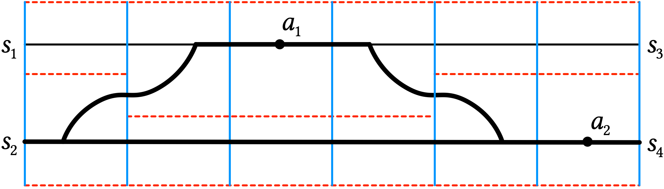
Figure 6. In this diagram, the bolded paths identify distinct witnesses to the causal relationship between initial site $s_{2}$ and final site $s_{4}$.

For example, the CSD depicted in Figure 6 goes from configuration $s_{1}\otimes s_{2}$ to configuration $s_{3}\otimes s_{4}$. Because $s_{2}$ is causally related to $s_{4}$ by two distinct paths, the type $s_{2}\rightsquigarrow s_{4}$ has two inhabitants.

4.2. Interior paths

Next, we will extend our spanning relation between bounding sites to a relation on all points of interest within a diagram. To do this, we need to refer not only to sites in the bounding configurations of $X$, but on any site configuration visited by $X$. A CSD with a sequence of $N$ global steps visits $N+1$ site configurations: one at the start of the diagram, and one at the end of each global step. Hence, an event will be a choice of site configuration in a diagram, together with a choice of site within that configuration.

Definition 4.3 (Cuts).

The type $\mathrm{Cut}(X)$ of cuts within a diagram $X:\Gamma_{1}\rightrightarrows\Gamma_{2}$ has one inhabitant for every site configuration visited by $X$, and is defined recursively over the structure of $X$. The associated function $\mathit{cut}(-)$ picks out the site configuration for each index of $\mathrm{Cut}(X)$.

$$\mathrm{Cut}(\mathbf{id}) =\top \mathit{cut}(\bullet) =\Gamma_{2}$$

$$\mathrm{Cut}(x\mathbin{;}y) =\mathrm{Cut}(x)+\top \mathit{cut}(\mathbf{inj}_{\ell}(t)) =\mathit{cut}(t) \mathit{cut}(\mathbf{inj}_{r}(\bullet)) =\Gamma_{2}$$

Definition 4.4 (Events).

The type $\mathrm{Event}(X)$ of events in a diagram $X$ is the type of points in spacetime consisting of a temporal coordinate (a cut) together with a spatial coordinate (a site):

$$\mathrm{Event}(X) =(t:\mathrm{Cut}(X),\ s:\mathrm{Site}(\mathit{cut}(t)))$$

This order of coordinates inverts the convention for events in a traditional execution, where we first select a process (a spatial coordinate) and then select an action occurring on that process (a temporal coordinate). In our figures (such as Figure 6), events exist wherever a line modeling the flow of data (in black) intersects a consistent cut (in blue).

Care should be taken not to confuse events with actions. In the traditional model of executions, an “event” is modeled by a local action — the equivalent of our $\mathbf{tick}$. However, since an action is effectively a discontinuous, instantaneous change to state, this leads to questions about what the state of a system is “at” a local action: Has the action actually happened yet or not? Is the action included in its own causal history? These ties are usually broken by interpreting events to occur either slightly before or slightly after an action — and sometimes both, depending on context. We prefer not to conflate these concepts in the first place: for us, an event is no more than a point in space at a point in time, with no presumption that it is special in any particular way.

Next, we need a way to describe paths between any two events. For any two cuts in a CSD, we can consider the global steps between them as a subdiagram. Then a path between two events is no more than a path spanning the subdiagram between their cuts. Order matters, however: if a CSD passes through distinct cuts $t_{1},t_{2}$ (in that order), the subdiagram “from $t_{2}$ to $t_{1}$” does not really exist — at least not in the expected sense. To preclude such inversions, we will define subdiagrams only over legal intervals.

Definition 4.5 (Intervals).

The interval $t_{1}\cdots t_{2}$ between cuts $t_{1},t_{2}$ in a diagram $X$ is the type with a (unique) inhabitant $t_{12}$ if and only if $X$ visits $t_{1}$ no later than $t_{2}$.

Definition 4.6 (The subdiagram over an interval).

The subdiagram over an interval $t_{12}:t_{1}\cdots t_{2}$, denoted $\mathit{during}(t_{12})$, is the CSD consisting of the global steps appearing strictly between cuts $t_{1},t_{2}$ in a diagram $X$.

Since CSDs are effectively (snoc-)lists at the top level, using $\mathit{during}(-)$ is akin to using the common list functions drop and take: we drop everything after both cuts, then take everything that remains after the first cut.

Finally, we can obtain a causal relation between events:

Definition 4.7 (Causal relations).

For a diagram $X$, a causal relation is a type family $\mathrm{Event}(X)\rightarrow\mathrm{Event}(X)\rightarrow\mathbf{Type}$ taking every pair of events to a type of relationships between them.

Definition 4.8 (Causal paths).

The type family $\rightsquigarrow$ of causal paths (sometimes interior paths) through a diagram $X$ is a causal relation. The inhabitants of $e_{1}\rightsquigarrow e_{2}$ are (dependent) pairs consisting of an interval between the events together with a spanning path under that interval:

$$(t_{1},s_{1})\rightsquigarrow(t_{2},s_{2})=(t_{12}:t_{1}\cdots t_{2},\ p_{12}:\mathrm{Span}(\mathit{during}(t_{12}))(s_{1},s_{2}))$$

We consistently pun $\rightsquigarrow$ to mean either spanning paths or causal paths depending on whether its arguments are sites or events. Similar liberties will be taken (and acknowledged) with the interpretations of Sections 5 and 6.

The causal relation $\rightsquigarrow$ enjoys reflexivity, antisymmetry, and transitivity, making it a partial order. As a proof-relevant type, reflexivity arises from the existence of unit paths, and transitivity arises from the composition of paths — which is, moreover, strictly associative. Unlike traditional executions (Definition 2.1), antisymmetry is guaranteed by construction for every CSD: it is impossible to introduce a causal loop because state flows only forward in time. Proofs of these properties can be found in our Agda development; we elide them here for brevity.

An order on actions

Here and in Section 2, we were careful to distinguish the actions related by happens-before from the spacetime coordinates we call events. Nonetheless, the two notions are closely related: every local action $a$ has a pair of associated events $e_{a}^{\ell},e_{a}^{r}$ before and after it. We can choose one of these events to act as proxy for the actions in our system to recover an irreflexive order on actions: $a_{i}<a_{j}$ if and only if $e_{a_{i}}^{r}\rightsquigarrow e_{a_{j}}^{\ell}$. For example, in Figure 6, we have $a_{1}<a_{2}$, since $e_{a_{1}}^{r}\rightsquigarrow e_{a_{2}}^{\ell}$. Because of this correspondence, we speak only of events in what follows — we can always choose a suitable event to stand in for any action of interest.

5. Interpreting CSDs into logical clocks

In this section (and Sections 6 and 7) we apply CSDs to the analysis of logical clocks, a common class of devices for reifying causal information into a concurrent system at runtime. As Lamport (1978) observed, we often cannot rely on physical timekeeping to coordinate agents in a concurrent system: one agent’s clock may drift relative to the others, and messages may take variable (or unbounded) amounts of time to propagate from sender to recipient. Logical clocks solve this problem by measuring time against the occurrence of intentional actions of the agents in the system.

In the setting of Lamport (1978), a logical clock (or just clock) is a global assignment of partially-ordered values (called timestamps) to actions in a concurrent execution. Figure 7 gives examples of these assignments for two widely used logical clocks: the scalar clock (Lamport, 1978) and the vector clock (Mattern, 1989; Fidge, 1988), which respectively use scalar and vector timestamps. We will discuss the specifics of these clocks in more detail in Section 7, along with matrix clocks (Wuu and Bernstein, 1984; Raynal et al., 1991).

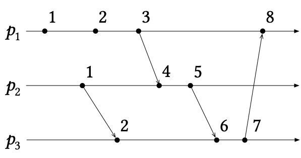
(a)   (b)

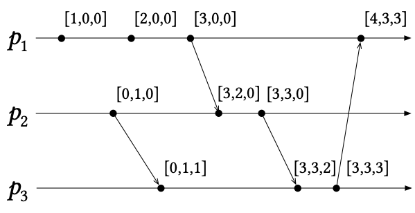
Figure 7. An example execution with an assignment of timestamps by the (a) Lamport clock and (b) vector clock.

In our setting, a clock will assign a timestamp to every event in a CSD. Just as in Section 4.2, we can assign timestamps to actions by choosing an adjacent event to represent that action.

We will use a common formulation of clocks as implementations of an abstract data type with local increment and merge operations (Raynal and Singhal, 1996), and we bridge this local characterization of clocks into a global assignment of timestamps via interpretation. We begin by justifying this choice of formulation; then, just as in the case of causal paths (Section 4), we construct an interpretation of CSDs $X:\Gamma_{1}\rightrightarrows\Gamma_{2}$ into a spanning domain, in which an assignment of timestamps (or “valuation”) on the sites of $\Gamma_{1}$ is updated into a valuation on $\Gamma_{2}$. We conclude by extending this interpretation to an interior domain, which will assign timestamps to all events within a diagram.

5.1. Realizable clocks

In practical implementations, a logical clock is realized as a data structure, instantiated by each agent in a concurrent system, that tracks the passage of (logical) time from the perspective of that agent. The timestamp associated to any action is that displayed by the clock of the agent when it performed the action. The archetypal logical clock is the scalar clock of (Lamport, 1978), in which every agent’s clock maintains a single monotonically-increasing integer. To ensure that every action occurs at a later “time” than those that occur causally prior, the scalar clock increments with each action, and updates to the maximum of its timestamp and that of any message received at that agent. This property — that causally-related actions have like-ordered timestamps — is so important that it is called the clock condition, and is required of any prospective logical clock.

While we can always build a global assignment of timestamps from a system of clock replicas, we cannot always go in the reverse direction: a clock in the global sense may not be realizable as a data structure. For instance, given an execution with $n$ actions, if $\mathcal{C}[-]$ is a monotone assignment of integer timestamps to this execution, then so is $\mathcal{C}[-]+n$. But an agent early in the execution has no knowledge of how many actions will occur in total: any prediction it makes may be invalidated depending on what transpires in the future. So even if $\mathcal{C}[-]$ can be realized as a system of local clock instances, $\mathcal{C}[-]+n$ certainly cannot be.

We restrict our attention to such realizable clocks, as these make up the majority of clocks in the literature. Following Raynal and Singhal (1996), we treat logical clocks as an abstract data type (ADT) with two operators, increment and merge. In addition, we assume a type $\mathrm{Act}$ of actions performable by any agent in the system.

Definition 5.1 (Clocks as an ADT).

A logical clock is a type $\mathrm{Time}$ together with

• a family of operations $\mathbf{increment}_{a}$ of type $\mathrm{Time}\rightarrow\mathrm{Time}$ for every $a:\mathrm{Act}$,

• an operation $\mathbf{\sqcup}$ (pronounced $\mathbf{merge}$) of type $\mathrm{Time}\times\mathrm{Time}\rightarrow\mathrm{Time}$.

Moreover, $\mathrm{Time}$ must be preordered by a relation $\leq$, such that for all timestamps $t_{1},t_{2}:\mathrm{Time}$, the above operations are inflationary:

• $t_{1}\leq\mathbf{increment}_{a}(t_{1})$,

• $t_{1}\leq(t_{1}\sqcup t_{2})$, and

• $t_{2}\leq(t_{1}\sqcup t_{2})$.

The $\mathbf{increment_{a}}$ operation advances the clock’s time depending on what the action $a$ is. For instance, a vector clock maintains an index for every agent, and it increments a different index depending on which agent performed the action. Since a CSD doesn’t carry information about the provenance of an action, we take the elements of $\mathrm{Act}$ to include that information themselves.

The $\mathbf{merge}$ operation advances the clock’s time to any time after the two given timestamps. This operation is used when an agent receives a message decorated with the sender’s timestamp: by merging the sender’s timestamp with the recipient’s timestamp, any action occuring from that point on is guaranteed to have a timestamp no less than than anything in its causal history.

5.2. Update functions

Given a logical clock, our goal is to derive a global assignment of timestamps to events for any CSD. Following the pattern in Section 3.4, we first restrict our attention to an assignment of timestamps to the bounding sites of an $\mathrm{Act}$-labeled diagram $X:\Gamma_{1}\rightrightarrows^{\mathrm{Act}}\Gamma_{2}$.

Intuitively, we will want to interpret every $\langle\mathbf{tick},a\rangle$ as an $\mathbf{increment}_{a}$ operation, and every $\langle\mathbf{join},\bullet\rangle$ as a $\mathbf{merge}$ over the input timestamps. An $\mathrm{Act}$-labeled CSD is then an expression arranging any number of clock operations on timestamps into a one-shot, compound operation over an entire configuration of clocks. In other words, every $\mathrm{Act}$-labeled CSD yields a function mapping an assignment of timestamps on its input sites to an assignment of timestamps on its output sites.

Definition 5.2 (Valuations).

The type of valuations on $\Gamma$, written $\mathrm{Valuation}(\Gamma)$, is the type of functions $\nu:\mathrm{Site}(\Gamma)\rightarrow\mathrm{Time}$ assigning a timestamp to each site in $\Gamma$.

Definition 5.3 (Update functions).

For every logical clock, the interpretation $\llbracket-\rrbracket$ of $\mathrm{Act}$-labeled CSDs $X:\Gamma_{1}\rightrightarrows^{\mathrm{Act}}\Gamma_{2}$ into update functions of type $\mathrm{Valuation}(\Gamma_{1})\rightarrow\mathrm{Valuation}(\Gamma_{2})$ is defined as:

$$\llbracket\mathbf{tick},\bullet\mapsto a\rrbracket =\lambda\nu.\ \lambda{-}.\ \mathbf{increment}(a)(\nu(\bullet))$$

$$\llbracket\mathbf{fork},{-}\rrbracket =\lambda\nu.\ \lambda{-}.\ \nu(\bullet)$$

$$\llbracket\mathbf{join},{-}\rrbracket =\lambda\nu.\ \lambda{-}.\ \nu(\mathbf{inj}_{\ell}(\bullet))\sqcup\nu(\mathbf{inj}_{r}(\bullet))$$

$$\llbracket\mathbf{perm}\ \sigma,{-}\rrbracket =\lambda\nu.\ \nu\circ\sigma^{-1} \llbracket\mathbf{id},{-}\rrbracket =\lambda\nu.\ \nu$$

$$\llbracket x\parallel y,f_{x}+f_{y}\rrbracket =\llbracket x,f_{x}\rrbracket+\llbracket y,f_{y}\rrbracket \llbracket x\mathbin{;}y,f_{x}+f_{y}\rrbracket =\llbracket y,f_{y}\rrbracket\circ\llbracket x,f_{x}\rrbracket$$

When the diagram $X$ is understood, we will write $\mathcal{C}_{\nu}[s]$ to mean $\llbracket X\rrbracket(\nu)(s)$.

Because a $\mathbf{tick}$ transforms a valuation on one site into a valuation on one site, it serves as a very thin wrapper around $\mathbf{increment}_{a}$. The new valuation can ignore its argument, because there is only one input to a $\mathbf{tick}$. Likewise, $\mathbf{fork}$ ignores its argument because both outputs receive their timestamp from the same input site, and $\mathbf{join}$ merges both input sites onto the single output site.

In contrast, the $\mathbf{perm}$ constructor doesn’t manipulate any timestamps directly. Instead, any given site is translated by the permutation $\sigma$ into an index on the input valuation: the requested timestamp is just one of those in the input. The $\mathbf{id}$ constructor behaves similarly.

Finally, sequential and concurrent composition each combine the evaluation functions from each subdiagram. Sequential composition is given by the usual composition of functions ($\circ$); and concurrent composition is given by the usual pairing of two functions over a sum type ($+$). We abuse pattern-matching notation somewhat by writing $f_{x}+f_{y}$ on the left-hand side, where we would otherwise write simply $f$ and compose its uses with the appropriate injection.

5.3. Clock functions

The interpretation of Definition 5.3 only tells us what timestamps a system terminates on, not the timestamps along the way. To obtain the latter, we must extend our function $\mathcal{C}_{\nu}$ to accept any event (Definition 4.4), not just output sites. That is, we want a function $\mathcal{C}:\mathrm{Valuation}(\Gamma_{1})\rightarrow(\mathrm{Event}(X)\rightarrow\mathrm{Time})$, computing an assignment of timestamps to all events given an initial assignment of timestamps.

Following Section 4.2, we will select a subdiagram with the event of interest on its boundary. The timestamp at an event is then one of the timestamps on which that subdiagram terminates.

Definition 5.4 (The subdiagram before a cut).

The subdiagram before a cut $t$, denoted $\mathit{before}(t)$, is the CSD consisting of the global steps appearing strictly before the cut $t$ in a diagram $X$.

Definition 5.5 (Clock function).

For every choice of logical clock and $\mathrm{Act}$-labeled diagram $X$, the clock function $\mathcal{C}$ of type $\mathrm{Valuation}(\Gamma_{1})\rightarrow(\mathrm{Event}(X)\rightarrow\mathrm{Time})$ is given by

$$\mathcal{C}_{\nu}[(t,s)] =\llbracket\mathit{before}(t)\rrbracket(\nu)(s).$$

We consistently pun $\mathcal{C}_{\nu}$ to mean either the update function (Definition 5.3) or the clock function depending on whether its argument is a site or an event.

Figure 8 depicts the execution from Figure 7 as a CSD, with timestamps assigned to events according to the Lamport clock, given a starting valuation of zeroes and using the interpretation in Definition 5.3. As discussed in Section 4.2, we can associate timestamps to actions rather than events just by selecting one of the neighboring events for each action to represent it. In this case, convention suggests adopting the timestamp of the event immediately following each action.

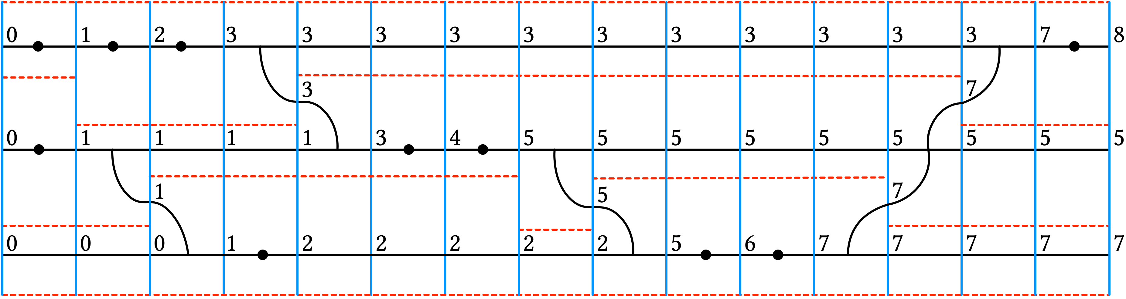
Figure 8. The execution from Figure 7 as a CSD, with Lamport timestamps assigned to events.

6. Relating causal paths to clocks

In Section 4, we introduced an interpretation into paths $e_{1}\rightsquigarrow e_{2}$, giving a proof-relevant causal order on events; and in Section 5, we introduced a family of interpretations into clock functions $\mathcal{C}_{\nu}[-]$, giving an assignment of timestamps to events. In this section, we will relate these two interpretation via a third, ultimately yielding a proof of the clock condition: if $e_{1}\rightsquigarrow e_{2}$, then $\mathcal{C}_{\nu}[e_{1}]\leq\mathcal{C}_{\nu}[e_{2}]$. Following the recipe in Section 3.4, we will again begin with a spanning proof relating paths and timestamps on the bounding sites, then extend to an interior proof relating paths and timestamps on all events.

6.1. Inflationarity of update functions

The clock condition relates any two events in a diagram: if $e_{1}\rightsquigarrow e_{2}$, then $\mathcal{C}_{\nu}[e_{1}]\leq\mathcal{C}_{\nu}[e_{2}]$. If we restrict our attention to sites $s_{1},s_{2}$ at the start and end of the diagram, respectively, then $\mathcal{C}_{\nu}[e_{1}]$ reduces to simply $\nu(s_{1})$, because the diagram before an initial site is the empty diagram $\mathbf{id}$. This leads us to the following statement:

Theorem 6.1 (The update function is inflationary).

Fix a choice of logical clock, and let $X$ be an $\mathrm{Act}$-labeled CSD $\Gamma_{1}\rightrightarrows^{\mathrm{Act}}\Gamma_{2}$ with an initial valuation $\nu:\mathrm{Valuation}(\Gamma_{1})$. Then the clock’s update function $\mathcal{C}$ is inflationary on causally related sites:

$$\forall(s_{1}:\mathrm{Site}(\Gamma_{1}))(s_{2}:\mathrm{Site}(\Gamma_{2}).\ (s_{1}\rightsquigarrow s_{2})\rightarrow(\nu(s_{1})\leq\mathcal{C}_{\nu}[s_{2}]).$$

This property is an analogue of the inflationary property satisfied by the clock operations of Definition 5.1: if an output can be influenced by an input, then the output must be bounded below by the input. In some ways, it would be surprising if Theorem 6.1 didn’t hold of $\mathcal{C}$, as it is built entirely from inflationary clock operations. Our proof will be built in kind, compsing proofs over atomic steps to yield proofs for entire diagrams. We sketch the proof at a high level here; the details are available in our Agda development.

• The proof for a $\mathbf{tick}$ step uses the fact that the clock’s $\mathbf{increment}$ operator is inflationary: $t\leq\textbf{increment}_{a}(t)$ for every action $a$ and timestamp $t$. This is true by construction for any clock implementing Definition 5.1.

• The proof for a $\mathbf{join}$ step uses the fact that the clock’s $\sqcup$ operator is inflationary on both arguments: both $t_{1}\leq(t_{1}\sqcup t_{2})$ and $t_{2}\leq(t_{1}\sqcup t_{2})$ for every pair of timestamps $t_{1}$, $t_{2}$. Again, this is definitionally true.

• The proof for a $\mathbf{fork}$ step uses the fact that the clock’s ordering relation is reflexive: we simply copy the input timestamp onto both outputs, so the actual values are unchanged. Indeed, this is true of $\mathbf{perm}$ and $\mathbf{id}$, too: all outputs are precisely the same as the (unique) inputs they are causally related to.

• The proof for a sequential composition ($\mathbin{;}$) uses the fact that the clock’s ordering relation is transitive. If we have a path through an intermediate site, where the time at the intermediate site is bounded below at the input and bounded above at the output, we must use transitivity to obtain a direct relationship between the input and output.

• The proof for a concurrent composition requires no information about the clock; however, the proof-relevance of our causal relation plays an essential role. We know that $s_{1}$ and $s_{2}$ are causally ordered because we were given a specific path witnessing the fact; and any given path through a concurrent composition is a path wholly through one concurrent half of the diagram or the other. Thus, we can simply dispatch to whichever sub-proof applies to the path at hand.

Somewhat surprisingly, nowhere do we require antisymmetry: even though partial orders are traditionally used in logical clocks, preorders are enough. This proof also holds for every CSD, even those not reflecting a well-behaved system. All we require is that updates are inflationary — the clock condition is not actually sensitive to what those updates are, or who performs them. This reveals a clean separation between clocks as ADTs and the protocols they are employed in; the clock condition is solely concerned with the ADT itself.

6.2. Monotonicity of clock functions

Just as in Sections 4.2 and 5.3, we need to be a little creative to leverage Theorem 6.1 into a proof of the full clock condition. The key insight is that, if we have a path of type $e_{1}\rightsquigarrow e_{2}$ and an initial valuation $\nu$, we can run the clock’s update function on the subdiagram before $e_{1}$. The resulting valuation is an initial valuation for the subdiagram between $e_{1}$ and $e_{2}$, on which we can apply inflationarity. Once more, we leave the finer details to our Agda implementation.

Theorem 6.2 (The clock function is monotonic).

Fix a choice of logical clock, and let $X$ be an $\mathrm{Act}$-labeled CSD $\Gamma_{1}\rightrightarrows^{\mathrm{Act}}\Gamma_{2}$ with an initial valuation $\nu:\mathrm{Valuation}(\Gamma_{1})$. Then the clock function $\mathcal{C}$ is monotonic on causally related events:

$$\forall(e_{1}\ e_{2}:\mathrm{Event}(X)).\ (e_{1}\rightsquigarrow e_{2})\rightarrow(\mathcal{C}_{\nu}[e_{1}]\leq\mathcal{C}_{\nu}[e_{2}]).$$

Theorem 6.2 tells us that every logical clock implementing the clock ADT of Definition 5.1 must necessarily satisfy the clock condition. In Section 7, we will actually instantiate these results on several clocks from the literature.

7. Verified logical clocks

In Sections 4, 5 and 6, we developed a framework for reasoning about causal relationships and logical clocks, culminating in a generic proof of the clock condition for implementations of the standard clock abstract data type. In this section we apply our results to several well-known clocks: Lamport’s scalar clock [(1978)], Mattern’s vector clock [(1989)], Raynal et al.’s matrix clock [(1991)], and Wuu and Bernstein’s matrix clock [Raynal et al.]. Implementations of these clocks are included in our Agda development, each with an instantiation of our generic proof of the clock condition.

Although there is only one “scalar” clock and “vector” clock in common use, there are two distinct “matrix” clocks with two-dimensional timestamps. The clock of Raynal et al., like the others we discuss, merges timestamps strictly pointwise; in contrast, the clock of Wuu and Bernstein (1984) additionally merges a row at one index into a row at another, yielding a noncommutative merge operator. To avoid confusion, we will refer to the former as the RST clock, and the latter as the Wuu-Bernstein clock. We will have more to say about the characteristics of the Wuu-Bernstein clock in Section 7.2; for now, we restrict our attention to the scalar, vector, and RST clocks.

7.1. Classifier clocks

The scalar, vector, and RST clocks all follow a similar template: we classify actions by some application-specific criterion, then maintain a count of observed actions for every class.

• The scalar clock classifies all actions into one single, universal class. Its timestamp consists of a single natural number, assessing a lower bound on the total number of actions that have occurred prior.

• The vector clock classifies actions based on who performed them, i.e. by actor. Its timestamp consists of a vector of natural numbers — or, equivalently, a function assigning a natural to every actor.

• The RST clock classifies actions based on subject and object: that is, every action is performed by some subject against some object. For Raynal et al. (1991), these actions are the submission of messages, where every message has both a sender (the subject) and a recipient (the object). The RST clock’s timestamp is thus a table counting messages sent between any two actors — or, equivalently, a function assigning a natural to every pair of actors.

Surprisingly, these clocks turn out to be structurally identical, differing only in their indexing classes $I$. In all cases, timestamps are maps $I\rightarrow\mathbb{N}$ ordered pointwise; the $\mathbf{increment}$ operation increments the value for a chosen class $i\in I$ by one; and the merge of two timestamps is their pointwise maximum. From elementary properties of natural numbers, this pointwise order is a preorder, and both operations are inflationary. Thus, we model all three clocks with one implementation, which we call a classifier clock, parametric in a classification function giving each action its class.

By instantiating Definition 5.5 and Theorem 6.2 on the classifier clock, we obtain a global assignment of timestamps for every CSD, together with a proof that this assignment is monotone (i.e., the clock condition). When specialized to sender-recipient classes (that is, indices $\mathrm{Pid}\times\mathrm{Pid}$), this yields the first mechanized proof (to our knowledge) of the clock condition for the RST clock.

7.2. Tensor clocks

The Wuu and Bernstein clock [(1984)] differs from the others in that it merges a row at the sender’s index into a row at the recipient’s, in addition to the usual pointwise merge. This merge operation is noncommutative, since it depends on which timestamp is considered the sender’s, and which is considered the recipient’s.

Kshemkalyani (2004) constructs a whole tensor clock hierarchy of clocks with noncommutative merge, where a general index $(c,o_{1},o_{2},\dots)$ models information of the form “$o_{1}$ knows that $o_{2}$ knows that $\dots$ $c$ occurred at least $N$ many times.” Clocks in this hierarchy model a kind of transitive knowledge: if one agent observes some population of actions, and they send a message to another agent, then the recipient transitively observes that same population of actions. The Wuu and Bernstein clock falls out as a special case of Kshemkalyani’s hierarchy.

We have implemented and verified the clock condition for the Wuu-Bernstein clock in our framework. However, the noncommutative merge operation poses some theoretical problems for the model of interpretation we developed in Section 5, which interprets the $\mathbf{join}$ atomic step into the clock’s merge operator. We want to treat $\mathbf{join}$ as commutative (up to isomorphism), as with the products of sets or types. Therefore, an interpretation via Definition 5.3 of $\mathbf{join}$ into a noncommutative merge operator would take equivalent CSDs to non-equivalent update functions. That said, since all such update functions are increasing, our proof of the clock condition in Theorem 6.2 still holds — there is no pair of equivalent CSDs for which the clock condition holds on one but not the other. Nonetheless, we hope to construct a more adequate interpretation that accounts for the full tensor clock hierarchy in the future.

8. Related work

MSCs and their semantics.

Message sequence charts (MSCs) are a diagrammatic language for representations of message-passing computations, widely used by practitioners and researchers (e.g., Lohrey and Muscholl (2004); Alur et al. (2000); Bollig et al. (2021); Di Giusto et al. (2023), as a small sampling). There have been various efforts to formalize MSCs or MSC-like diagrammatic languages, including the MSC standard itself (ITU-T, 2011) and others (Schätz et al., 1996), and investigations of the semantics of MSCs (Ladkin and Leue, 1993; Broy, 2005; Alur et al., 1996; Mauw and Reniers, 1994; Gehrke et al., 1998). However, we are not aware of any formalizations of MSCs that define them inductively, as we have done for CSDs. Rather, existing MSC formalizations are in terms of a given set of messages and a given set of processes.

Alur et al. (1996) note that MSCs admit “a variety of semantic interpretations”, seemingly similar in spirit to our interpretations of CSDs. However, Alur et al.’s interpretations yield refinements of causal order – for example, they note that the meaning of a given MSC may depend on the choice of network model and fault model (e.g., whether message loss or reordering are possible). While we give an interpretation of CSDs into a causal order, our range of possible semantic domains is greater: we also give interpretations into computable functions and into proofs.

Mechanized reasoning about clocks and causality in concurrent systems.

In distributed systems, the notion of causal ordering arises in a myriad of settings, including causally consistent data stores (Ahamad et al., 1995; Lloyd et al., 2011), distributed snapshot protocols (Mattern, 1989; Acharya and Badrinath, 1992; Alagar and Venkatesan, 1994), causal message delivery protocols (Birman and Joseph, 1987a; Schiper et al., 1989; Birman and Joseph, 1987b; Birman et al., 1991), and conflict-free replicated data types (CRDTs) (Shapiro et al., 2011). In shared-memory systems, the need to reason about causality arises in the setting of data race detection for multithreaded programs (Pozniansky and Schuster, 2003; Flanagan and Freund, 2009). It is typical for such applications to use logical clocks of one kind or another to reify causal information.

There are several mechanically verified implementations of distributed algorithms that use logical clocks (Lesani et al., 2016; Gondelman et al., 2021; Nieto et al., 2022; Redmond et al., 2023). These proof developments focus on verifying properties of those higher-level algorithms (such as causal consistency of replicated databases (Lesani et al., 2016; Gondelman et al., 2021), convergence of CRDTs (Nieto et al., 2022), or safety of causal message broadcast (Nieto et al., 2022; Redmond et al., 2023)), and they (implicitly or explicitly) take the clock condition as an axiom.

The only other work that we are aware of on mechanized verification of the clock condition itself is by Mansky et al. (2017), whose work focuses on the verification of dynamic race detection algorithms. As part of their larger proof development, Mansky et al. proved in Coq that vector clocks precisely characterize the causal order. That is, they proved not only the clock condition for vector clocks, as we do here, but also the inverse clock condition: if $e_{i}$’s timestamp is less than $e_{j}$’s timestamp, then $e_{i}$ causally precedes $e_{j}$. Unlike the (forward) clock condition, the inverse clock condition depends on the particular protocol governing use of the clock: a process must not increment an index owned by another process. While our proof development works for any clock that can be expressed as an ADT, we cannot yet prove protocol-dependent properties like the inverse clock condition. We hope to approach such properties in future work.

Separation logics.

Separation logics (Reynolds, 2002) are program logics for reasoning about the correct use of resources — concrete resources such as memory, but, excitingly, also logical resources such as permissions and execution history. Concurrent separation logics (O’Hearn, 2007) enable such reasoning about concurrent programs. The literature on separation logics and concurrent separation logics is too vast to summarize here, although O’Hearn (2019) offers an accessible introduction and Brookes and O’Hearn (2016) give an overview of important developments. CSDs are heavily inspired by concurrent separation logic, but we have not yet pursued a program logic based on CSDs. Wickerson et al. (2013)’s ribbon proofs, a diagrammatic proof system based on separation logic, could be an inspiration for future work in this direction.

Separation logic has been used in the service of reasoning about causality. Gondelman et al. (2021) and Nieto et al. (2022) both use the Aneris concurrent separation logic framework (Krogh-Jespersen et al., 2020), itself built on the Iris (Jung et al., 2018) framework, to verify the correctness of distributed systems in which causality is a central concern. However, the Aneris framework does not offer any particular support for reasoning about causality. In fact, we are not aware of program logics or verification frameworks that are specifically intended for reasoning about causality, which is perhaps surprising, considering the importance of causality in concurrent systems. Rather than reasoning about causal relationships as logical resources, as one would do when using Iris or Aneris, causality in a CSD-based proof system would manifest in the structure of the proof itself.

String diagrams.

Our CSDs are inspired by the string diagrams employed in category theory, which formally describe compositions of morphisms in a monoidal category (i.e., with a concurrent composition operator) using a graphical syntax. The standard reference for string diagrams is Joyal and Street (1991), though Piedeleu and Zanasi (2023) give an accessible introduction for computer scientists. We hope to establish firmer connections between CSDs and string diagrams in future work, e.g., by proving that CSDs form a (symmetric) monoidal category. Moreover, recent work by Nester (2021) has described execution traces in concurrent systems using string diagrams in which data can be transferred between tiles both in time (in the forward direction) and in space (in the sideways direction). This contrasts with our CSDs, in which data is only transferred in time. Nester leverages double categories to formalize these two-dimensional interfaces. It would be interesting to investigate what a treatment of causality might look like in such a setting.

A completely different application of string diagrams can be found in the tape diagrams of Bonchi et al. (2023), which give a graphical syntax to set-theoretic relations. A tape diagram is a two-layer presentation of relations, with disjunction on one layer and conjunction on another. The two-layer structure of CSDs, with global actions over global state decomposing into local actions over local state, is reminiscent of Bonchi et al.’s approach. We would like to explore the connections between these ideas in future work.

9. Conclusion

Causality is of central importance in concurrent systems, including both shared-state and message-passing systems. In this paper, we presented causal separation diagrams (CSDs), a new formal model of concurrent executions that is inductively defined and enjoys a diagrammatic syntax reminiscent of Lamport diagrams. The inductive nature of CSDs makes them amenable to mechanized reasoning and interpretation.

As a case study, we used CSDs to reason about logical clocks, ubiquitous mechanisms for reifying causal information in concurrent systems. By interpretating CSDs into a variety of semantic domains, we built up a generic proof of Lamport’s clock condition that holds for any realizable logical clock, including the Wuu-Bernstein clock and the RST clock, neither of which were mechanically verified previously. A proof-relevant analogue of Lamport’s happens-before relation, witnessing concrete causal paths in an execution, plays an essential role in these proofs. Our framework and results are available as an Agda development.

While logical clocks were a focus of this paper, we see CSDs (and interpretations of CSDs) as a valuable reasoning tool beyond their application to logical clocks. In future work, we hope to flesh out the connection between CSDs and symmetric monoidal categories in more detail, including notions of equivalence and refinement for CSDs, which will hopefully yield well-behavedness conditions for interpretations.

References

- (1)
- Acharya and Badrinath (1992) Arup Acharya and B.R. Badrinath. 1992. Recording distributed snapshots based on causal order of message delivery. Inform. Process. Lett. 44, 6 (1992), 317–321. https://doi.org/10.1016/0020-0190(92)90107-7
- Ahamad et al. (1995) Mustaque Ahamad, Gil Neiger, James E. Burns, Prince Kohli, and Phillip W. Hutto. 1995. Causal memory: definitions, implementation, and programming. Distributed Computing 9, 1 (1995), 37–49. https://doi.org/10.1007/BF01784241
- Alagar and Venkatesan (1994) Sridhar Alagar and S. Venkatesan. 1994. An optimal algorithm for distributed snapshots with causal message ordering. Inform. Process. Lett. 50, 6 (1994), 311–316. https://doi.org/10.1016/0020-0190(94)00055-7
- Altenkirch and Morris (2009) Thorsten Altenkirch and Peter Morris. 2009. Indexed Containers. In 2009 24th Annual IEEE Symposium on Logic In Computer Science. 277–285. https://doi.org/10.1109/lics.2009.33
- Alur et al. (2000) Rajeev Alur, Kousha Etessami, and Mihalis Yannakakis. 2000. Inference of Message Sequence Charts. In Proceedings of the 22nd International Conference on Software Engineering (Limerick, Ireland) (ICSE ’00). Association for Computing Machinery, New York, NY, USA, 304–313. https://doi.org/10.1145/337180.337215
- Alur et al. (1996) Rajeev Alur, Gerard J. Holzmann, and Doron Peled. 1996. An analyzer for message sequence charts. In Tools and Algorithms for the Construction and Analysis of Systems, Tiziana Margaria and Bernhard Steffen (Eds.). Springer Berlin Heidelberg, Berlin, Heidelberg, 35–48.
- Birman and Joseph (1987a) K. Birman and T. Joseph. 1987a. Exploiting Virtual Synchrony in Distributed Systems. SIGOPS Oper. Syst. Rev. 21, 5 (Nov. 1987), 123–138. https://doi.org/10.1145/37499.37515
- Birman et al. (1991) Kenneth Birman, André Schiper, and Pat Stephenson. 1991. Lightweight Causal and Atomic Group Multicast. ACM Trans. Comput. Syst. 9, 3 (Aug. 1991), 272–314. https://doi.org/10.1145/128738.128742
- Birman and Joseph (1987b) Kenneth P. Birman and Thomas A. Joseph. 1987b. Reliable Communication in the Presence of Failures. ACM Trans. Comput. Syst. 5, 1 (Jan. 1987), 47–76. https://doi.org/10.1145/7351.7478
- Bollig et al. (2021) Benedikt Bollig, Cinzia Di Giusto, Alain Finkel, Laetitia Laversa, Etienne Lozes, and Amrita Suresh. 2021. A Unifying Framework for Deciding Synchronizability. In 32nd International Conference on Concurrency Theory (CONCUR 2021) (Leibniz International Proceedings in Informatics (LIPIcs), Vol. 203), Serge Haddad and Daniele Varacca (Eds.). Schloss Dagstuhl – Leibniz-Zentrum für Informatik, Dagstuhl, Germany, 14:1–14:18. https://doi.org/10.4230/LIPIcs.CONCUR.2021.14
- Bonchi et al. (2023) Filippo Bonchi, Alessandro Di Giorgio, and Alessio Santamaria. 2023. Deconstructing the Calculus of Relations with Tape Diagrams. Proc. ACM Program. Lang. 7, POPL, Article 64 (Jan. 2023), 31 pages. https://doi.org/10.1145/3571257
- Brookes and O’Hearn (2016) Stephen Brookes and Peter W. O’Hearn. 2016. Concurrent Separation Logic. ACM SIGLOG News 3, 3 (aug 2016), 47–65. https://doi.org/10.1145/2984450.2984457
- Broy (2005) Manfred Broy. 2005. A semantic and methodological essence of message sequence charts. Science of Computer Programming 54, 2 (2005), 213–256. https://doi.org/10.1016/j.scico.2004.04.003
- Castro and Liskov (1999) Miguel Castro and Barbara Liskov. 1999. Practical Byzantine Fault Tolerance. In Proceedings of the Third Symposium on Operating Systems Design and Implementation (New Orleans, Louisiana, USA) (OSDI ’99). USENIX Association, Usa, 173–186.
- Chandy and Lamport (1985) K. Mani Chandy and Leslie Lamport. 1985. Distributed Snapshots: Determining Global States of Distributed Systems. ACM Trans. Comput. Syst. 3, 1 (Feb. 1985), 63–75. https://doi.org/10.1145/214451.214456
- Di Giusto et al. (2023) Cinzia Di Giusto, Davide Ferré, Laetitia Laversa, and Etienne Lozes. 2023. A Partial Order View of Message-Passing Communication Models. Proc. ACM Program. Lang. 7, POPL, Article 55 (Jan. 2023), 27 pages. https://doi.org/10.1145/3571248
- Ellis and Gibbs (1989) C. A. Ellis and S. J. Gibbs. 1989. Concurrency Control in Groupware Systems. SIGMOD Rec. 18, 2 (June 1989), 399–407. https://doi.org/10.1145/66926.66963
- Fidge (1988) C. J. Fidge. 1988. Timestamps in message-passing systems that preserve the partial ordering. Proceedings of the 11th Australian Computer Science Conference 10, 1 (1988), 56–66.
- Flanagan and Freund (2009) Cormac Flanagan and Stephen N. Freund. 2009. FastTrack: Efficient and Precise Dynamic Race Detection. In Proceedings of the 30th ACM SIGPLAN Conference on Programming Language Design and Implementation (Dublin, Ireland) (PLDI ’09). Association for Computing Machinery, New York, NY, USA, 121–133. https://doi.org/10.1145/1542476.1542490
- Gehrke et al. (1998) Thomas Gehrke, Michaela Huhn, Arend Rensink, and Heike Wehrheim. 1998. An Algebraic Semantics for Message Sequence Chart Documents. Springer US, Boston, MA, 3–18. https://doi.org/10.1007/978-0-387-35394-4_1
- Gondelman et al. (2021) Léon Gondelman, Simon Oddershede Gregersen, Abel Nieto, Amin Timany, and Lars Birkedal. 2021. Distributed Causal Memory: Modular Specification and Verification in Higher-Order Distributed Separation Logic. Proc. ACM Program. Lang. 5, POPL, Article 42 (Jan. 2021), 29 pages. https://doi.org/10.1145/3434323
- ITU-T (2011) ITU-T. 2011. ITU Recommendation Z.120: Message Sequence Chart (MSC). https://www.itu.int/rec/T-REC-Z.120-201102-I/
- Joyal and Street (1991) André Joyal and Ross Street. 1991. The geometry of tensor calculus, I. Advances in Mathematics 88, 1 (July 1991), 55–112. https://doi.org/10.1016/0001-8708(91)90003-p
- Jung et al. (2018) Ralf Jung, Robbert Krebbers, Jacques-Henri Jourdan, Ales Bizjak, Lars Birkedal, and Derek Dreyer. 2018. Iris from the ground up: A modular foundation for higher-order concurrent separation logic. J. Funct. Program. 28 (2018), e20. https://doi.org/10.1017/S0956796818000151
- Krogh-Jespersen et al. (2020) Morten Krogh-Jespersen, Amin Timany, Marit Edna Ohlenbusch, Simon Oddershede Gregersen, and Lars Birkedal. 2020. Aneris: A Mechanised Logic for Modular Reasoning about Distributed Systems. In Programming Languages and Systems: 29th European Symposium on Programming, ESOP 2020, Held as Part of the European Joint Conferences on Theory and Practice of Software, ETAPS 2020, Dublin, Ireland, April 25–30, 2020, Proceedings (Dublin, Ireland). Springer-Verlag, Berlin, Heidelberg, 336–365. https://doi.org/10.1007/978-3-030-44914-8_13
- Kshemkalyani (2004) Ajay D. Kshemkalyani. 2004. The power of logical clock abstractions. Distributed Computing 17, 2 (Aug. 2004). https://doi.org/10.1007/s00446-003-0105-9
- Ladkin and Leue (1993) Peter B. Ladkin and Stefan Leue. 1993. What Do Message Sequence Charts Mean?. In Proceedings of the IFIP TC6/WG6.1 Sixth International Conference on Formal Description Techniques, VI (Forte ’93). North-Holland Publishing Co., Nld, 301–316.
- Lamport (1978) Leslie Lamport. 1978. Time, Clocks, and the Ordering of Events in a Distributed System. Commun. ACM 21, 7 (July 1978), 558–565. https://doi.org/10.1145/359545.359563
- Le Lann (1977) Gérard Le Lann. 1977. Distributed Systems – Toward a Formal Approach. In Proceedings of IFIP Congress 1977 (Toronto, Canada) (Ifip ’77). North-Holland Publishing Co., Nld, 155–160.
- Lesani et al. (2016) Mohsen Lesani, Christian J. Bell, and Adam Chlipala. 2016. Chapar: Certified Causally Consistent Distributed Key-Value Stores. In Proceedings of the 43rd Annual ACM SIGPLAN-SIGACT Symposium on Principles of Programming Languages (St. Petersburg, FL, USA) (POPL ’16). Association for Computing Machinery, New York, NY, USA, 357–370. https://doi.org/10.1145/2837614.2837622
- Lloyd et al. (2011) Wyatt Lloyd, Michael J. Freedman, Michael Kaminsky, and David G. Andersen. 2011. Don’t Settle for Eventual: Scalable Causal Consistency for Wide-Area Storage with COPS. In Proceedings of the Twenty-Third ACM Symposium on Operating Systems Principles (Cascais, Portugal) (SOSP ’11). Association for Computing Machinery, New York, NY, USA, 401–416. https://doi.org/10.1145/2043556.2043593
- Lohrey and Muscholl (2004) Markus Lohrey and Anca Muscholl. 2004. Bounded MSC communication. Information and Computation 189, 2 (2004), 160–181. https://doi.org/10.1016/j.ic.2003.10.002
- Mansky et al. (2017) William Mansky, Yuanfeng Peng, Steve Zdancewic, and Joseph Devietti. 2017. Verifying Dynamic Race Detection. In Proceedings of the 6th ACM SIGPLAN Conference on Certified Programs and Proofs (Paris, France) (Cpp 2017). Association for Computing Machinery, New York, NY, USA, 151–163. https://doi.org/10.1145/3018610.3018611
- Mathur et al. (2022) Umang Mathur, Andreas Pavlogiannis, Hünkar Can Tunç, and Mahesh Viswanathan. 2022. A Tree Clock Data Structure for Causal Orderings in Concurrent Executions. In Proceedings of the 27th ACM International Conference on Architectural Support for Programming Languages and Operating Systems (Lausanne, Switzerland) (ASPLOS ’22). Association for Computing Machinery, New York, NY, USA, 710–725. https://doi.org/10.1145/3503222.3507734
- Mattern (1989) Friedemann Mattern. 1989. Virtual Time and Global States of Distributed Systems. In Parallel and Distributed Algorithms. North-Holland, 215–226.
- Mauw and Reniers (1994) S. Mauw and M. A. Reniers. 1994. An Algebraic Semantics of Basic Message Sequence Charts. Comput. J. 37, 4 (01 1994), 269–277. https://doi.org/10.1093/comjnl/37.4.269
- Nester (2021) Chad Nester. 2021. The Structure of Concurrent Process Histories. In Coordination Models and Languages (Lecture Notes in Computer Science), Ferruccio Damiani and Ornela Dardha (Eds.). Springer International Publishing, Cham, 209–224. https://doi.org/10.1007/978-3-030-78142-2_13
- Nieto et al. (2022) Abel Nieto, Léon Gondelman, Alban Reynaud, Amin Timany, and Lars Birkedal. 2022. Modular Verification of Op-Based CRDTs in Separation Logic. Proc. ACM Program. Lang. 6, OOPSLA2, Article 188 (Oct. 2022), 29 pages. https://doi.org/10.1145/3563351
- O’Hearn (2019) Peter O’Hearn. 2019. Separation Logic. Commun. ACM 62, 2 (jan 2019), 86–95. https://doi.org/10.1145/3211968
- O’Hearn (2007) Peter W. O’Hearn. 2007. Resources, concurrency, and local reasoning. Theoretical Computer Science 375, 1 (2007), 271–307. https://doi.org/10.1016/j.tcs.2006.12.035 Festschrift for John C. Reynolds’s 70th birthday.
- Piedeleu and Zanasi (2023) Robin Piedeleu and Fabio Zanasi. 2023. An Introduction to String Diagrams for Computer Scientists. arXiv:2305.08768 [cs.LO] https://arxiv.org/abs/2305.08768
- Pozniansky and Schuster (2003) Eli Pozniansky and Assaf Schuster. 2003. Efficient On-the-Fly Data Race Detection in Multithreaded C++ Programs. In Proceedings of the Ninth ACM SIGPLAN Symposium on Principles and Practice of Parallel Programming (San Diego, California, USA) (PPoPP ’03). Association for Computing Machinery, New York, NY, USA, 179–190. https://doi.org/10.1145/781498.781529
- Raynal et al. (1991) Michel Raynal, André Schiper, and Sam Toueg. 1991. The causal ordering abstraction and a simple way to implement it. Inform. Process. Lett. 39, 6 (Sept. 1991), 343–350. https://doi.org/10.1016/0020-0190(91)90008-6
- Raynal and Singhal (1996) Michel Raynal and Mukesh Singhal. 1996. Logical time: Capturing causality in distributed systems. Computer 29, 2 (1996), 49–56.
- Redmond et al. (2023) Patrick Redmond, Gan Shen, Niki Vazou, and Lindsey Kuper. 2023. Verified Causal Broadcast with Liquid Haskell. In Proceedings of the 34th Symposium on Implementation and Application of Functional Languages (Copenhagen, Denmark) (IFL ’22). Association for Computing Machinery, New York, NY, USA, Article 6, 13 pages. https://doi.org/10.1145/3587216.3587222
- Reynolds (2002) J.C. Reynolds. 2002. Separation logic: a logic for shared mutable data structures. In Proceedings 17th Annual IEEE Symposium on Logic in Computer Science. 55–74. https://doi.org/10.1109/LICS.2002.1029817
- Schätz et al. (1996) Bernhard Schätz, Heinrich Hußmann, and Manfred Broy. 1996. Graphical development of consistent system specifications. In FME’96: Industrial Benefit and Advances in Formal Methods, Marie-Claude Gaudel and James Woodcock (Eds.). Springer Berlin Heidelberg, Berlin, Heidelberg, 248–267.
- Schiper et al. (1989) André Schiper, Jorge Eggli, and Alain Sandoz. 1989. A New Algorithm to Implement Causal Ordering. In Proceedings of the 3rd International Workshop on Distributed Algorithms. Springer-Verlag, Berlin, Heidelberg, 219–232.
- Shapiro et al. (2011) Marc Shapiro, Nuno Preguiça, Carlos Baquero, and Marek Zawirski. 2011. Conflict-Free Replicated Data Types. In Proceedings of the 13th International Conference on Stabilization, Safety, and Security of Distributed Systems (Grenoble, France) (SSS’11). Springer-Verlag, Berlin, Heidelberg, 386–400.
- Weil et al. (2006) Sage A. Weil, Scott A. Brandt, Ethan L. Miller, Darrell D. E. Long, and Carlos Maltzahn. 2006. Ceph: A Scalable, High-Performance Distributed File System. In Proceedings of the 7th Symposium on Operating Systems Design and Implementation (Seattle, Washington) (OSDI ’06). USENIX Association, USA, 307–320.
- Wickerson et al. (2013) John Wickerson, Mike Dodds, and Matthew J. Parkinson. 2013. Ribbon Proofs for Separation Logic. In Programming Languages and Systems - 22nd European Symposium on Programming, ESOP 2013, Held as Part of the European Joint Conferences on Theory and Practice of Software, ETAPS 2013, Rome, Italy, March 16-24, 2013. Proceedings (Lecture Notes in Computer Science, Vol. 7792), Matthias Felleisen and Philippa Gardner (Eds.). Springer, 189–208. https://doi.org/10.1007/978-3-642-37036-6_12
- Wuu and Bernstein (1984) Gene T.J. Wuu and Arthur J. Bernstein. 1984. Efficient Solutions to the Replicated Log and Dictionary Problems. In Proceedings of the Third Annual ACM Symposium on Principles of Distributed Computing (Vancouver, British Columbia, Canada) (PODC ’84). Association for Computing Machinery, New York, NY, USA, 233–242. https://doi.org/10.1145/800222.806750