Embedded coherent structures from MHD to sub-ion scales in turbulent solar wind at 0.17 AU

Abstract

We study solar wind magnetic turbulence with Parker Solar Probe during its first perihelion (at 0.17 au), from MHD to kinetic plasma scales. Using Morlet wavelet decomposition, we detect intermittent coherent structures, appearing as localized in time energetic events and covering a large range of scales. This implies the presence of embedded coherent structures from MHD down to sub-ion scales. For example, we observe a current sheet at MHD scales ($\sim 200$ s) with magnetic fluctuations inherent for a magnetic vortex at ion scales ($\sim 1$ s) and at sub-ion scales ($\sim 0.1$ s). The amplitude anisotropy of magnetic fluctuations is analyzed within nearly (i) 200 structures at MHD scales, (ii) $\sim 2\cdot 10^{3}$ events at ion scales and (iii) $\sim 10^{4}$ events at sub-ion scales. We compare it with crossings of model structures, such as Alfvén vortices, current sheets and magnetic holes, along the trajectories with various impact parameters.

From this comparison, we conclude that at MHD and ion scales the majority of the structures are incompressible and represent mainly dipole Alfvén vortices (>80%), monopole Alfvén vortices (<10%) and current sheets (<10%). On subion scales coherent structures represent monopole vortices (7%), dipole vortices (49%) current sheets (5%) and magnetic holes (0.4%). Around 40 % of structures at sub-ion scales don’t fit any of the considered models. These events might represent compressible vortices.

1 Introduction

Solar wind fluctuations cover a broad range of scales: from macroscopic scales, where the energy is injected into the MHD turbulent cascade, to micro-scales, where kinetic effects play important role, and the energy is dissipated. The dissipation mechanism has not been understood yet. Numerical simulations indicate that dissipation occurs inhomogeneously (Wan et al., 2012; Karimabadi et al., 2013; Zhdankin et al., 2013; Kuzzay et al., 2019). Regions of increased heating in the solar wind correlate with observations of coherent structures (Osman et al., 2011; Wu et al., 2013; Chasapis et al., 2015; Sioulas et al., 2022). Coherent structures can be defined as high-amplitude, stable, localized in space events with phase coherence over its spatial extent (Hussain, 1986; Fiedler, 1988; Veltri, 1999; Bruno et al., 2001; Mangeney, 2001; Farge & Schneider, 2015; Alexandrova, 2020).

Different types of coherent structures are observed in the solar wind at different scales. Large scale flux tubes and flux ropes cover energy containing scales and the inertial range (e.g. Moldwin et al., 2000; Feng et al., 2008; Borovsky, 2008; Janvier et al., 2014; Zhao et al., 2020). Current sheets are usually observed at small scales of the inertial range and at ion scales (e.g. Siscoe et al., 1968; Burlaga, 1969; Salem, 2000; Knetter et al., 2004; Tsurutani et al., 2011; Lion et al., 2016; Perrone et al., 2016; Artemyev et al., 2019). Recent Solar Orbiter observations reveal embedded ion scale flux rope in a bifurcated current sheet (Eastwood et al., 2021). Alfvén vortices have been identified at MHD scales and at ion scales (Verkhoglyadova et al., 2003; Roberts et al., 2016; Lion et al., 2016; Perrone et al., 2016, 2017). Compressible structures, such as magnetic holes (e.g. Turner et al., 1977; Stevens & Kasper, 2007; Volwerk et al., 2020)), solitons and shocks (Perrone et al., 2016; Salem, 2000) are observed at the end of the inertial range and at ion scales.

Coherent structures contribute significantly to the magnetic turbulent spectrum in the solar wind. Li et al. (2011) show that in the presence of current sheets, the inertial range spectrum is closer to the Kolmogorov scaling, $-5/3$, while without current sheets, the spectrum is closer to the Iroshnikov-Kraichnan scaling, $-3/2$. In a case study of a fast wind stream by Lion et al. (2016), the contribution of coherent structures to magnetic field spectrum is up to 40 % from inertial range down to ion scales. Therefore, coherent structures are energetically important elements of solar wind turbulence.

Much less observations of coherent structures exist at sub-ion scales. Cluster/STAFF allows to measure sub-ion scale fluctuations at 1 au. Greco et al. (2016) studied ion scales current sheets and showed presence of a number of smaller ones at sub-ion scales. This has been done using the partial variance of increments (PVI) method (Greco et al., 2018), which is appropriate to detect planar structures with important field rotation (e.g., see the discussion in Lion et al., 2016). Another study with Cluster, but applying Morlet wavelets show embedded Alfvén vortex type fluctuations at sub-ion scales in a current sheet at ion scales (Jovanović et al., 2018). An analytic model of a chain of Alfvén vortices embedded in the current sheet is developed by authors.

First multi-satellite observation of these cylindrical structures have been done in the Earth’s magnetosheath with the Cluster mission (Alexandrova et al., 2006; Alexandrova, 2008). Cassini measurements indicate the presence of such structures in the Kronian magnetosheath as well (Alexandrova & Saur, 2008). Signatures of Alfvén vortices in the solar wind using one satellite have been shown by Verkhoglyadova et al. (2003); Lion et al. (2016). Roberts et al. (2016) and Perrone et al. (2016, 2017) confirmed the existence of Alfven vortices in the solar wind with 4 satellites of Cluster. Wang et al. (2019) investigated the kinetic effects within an Alfvén vortex thanks to MMS measurements in the Earth’s magnetosheath.

In the present paper, we study magnetic turbulent fluctuations from MHD inertial range to sub-ion scales with Parker Solar Probe (PSP) data at 0.17 au. Using the Morlet wavelet transform, which is a good compromise between time and frequency resolution, we detect intermittent events which cover a wide range of scales. We show that these events correspond to embedded multi scale structures, from MHD to sub-ion scales. Then, we study in more details nature of these structures, which cover the whole turbulent cascade.

The article is organized as follows: Section 2 describes the PSP data used in the analysis. In Section 3 magnetic spectral properties are discussed. Section 4 is dedicated to the detection method of coherent structures. Section 5 presents several theoretical models of the structures we think we cross by PSP at different scales. Then we study the sensitivity of minimum variance results for different spacecraft trajectories across the model structures for different noise levels. In section 6 we describe few examples of detected structures at MHD, ion and sub-ion scales simultaneously. Section 7 describes statistical study of the observed coherent events during 5h of the 1st PSP encounter at MHD, ion and sub-ion scales. In section 8 we summarize and discuss the results.

2 Data

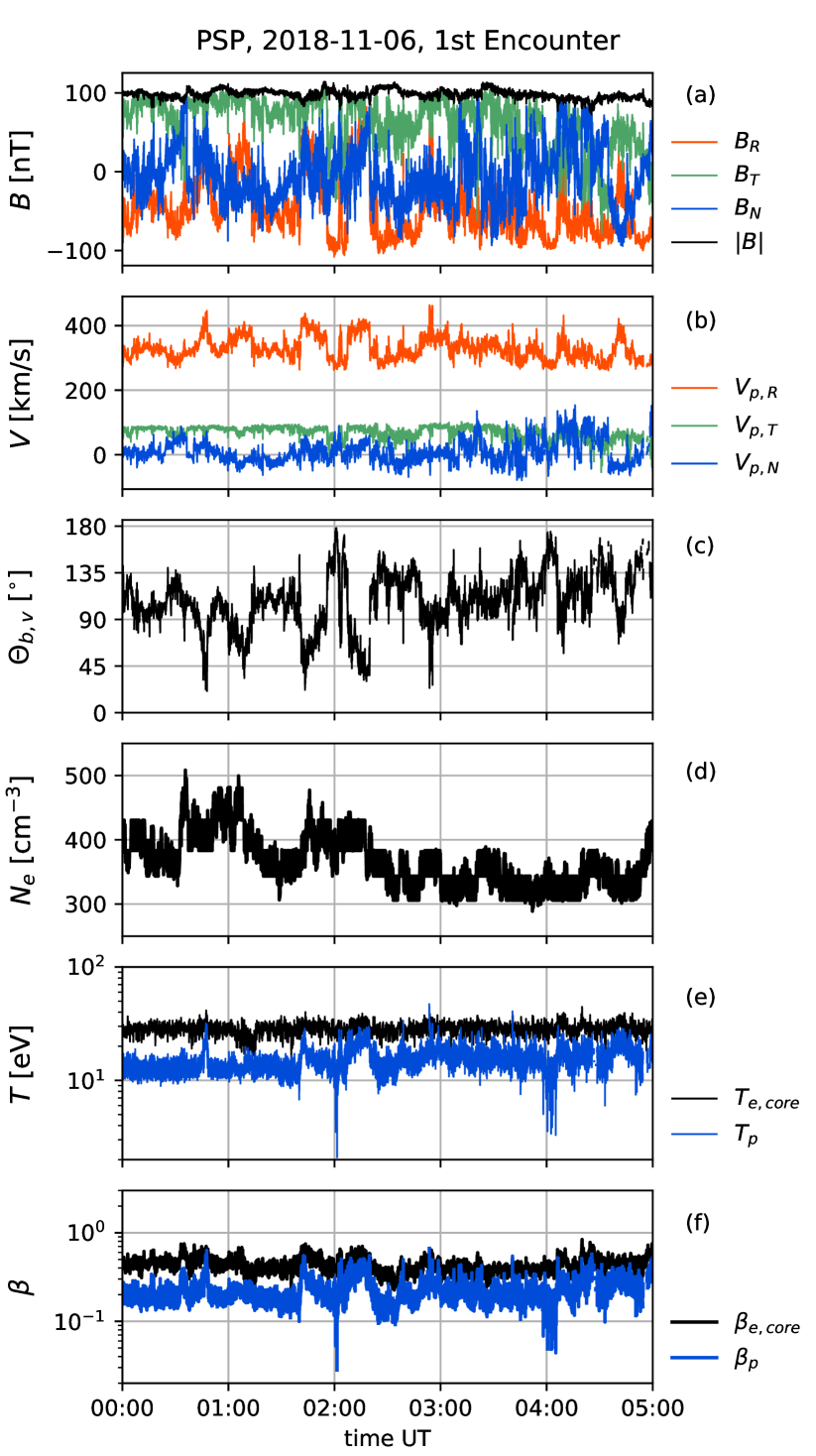
Figure 1: Overview of the solar wind data during the first perihelion of PSP at 0.17 au on November 6, 2018, between 00:00 and 05:00 UT. From top to bottom: (a) the magnetic field components in RTN reference frame and the magnetic field modulus, (b) proton bulk velocity components, (c) angle between the magnetic field and the proton bulk velocity, (d) electron density, (e) proton temperature (in blue) and core electron temperatures (in black), (f) core electron and proton plasma beta.

We analyze 5 hours time interval during the first perihelion, on November 6, 2018, [00:00, 05:00] UT, when the spacecraft measured the solar wind emerging from the small equatorial coronal hole at the distance of 0.17 au from the Sun (Bale et al., 2019; Kasper et al., 2019). The magnetic field during the chosen time interval is particularly highly-disturbed due to the presence of high-amplitude structures (including switchbacks, Bale et al., 2019; Perrone et al., 2020). The duration of the chosen interval is long enough to resolve the inertial range of MHD turbulence, but not too long, so that the PSP is magnetically connected to the same coronal hole and the PSP position is nearly at the same radial distance from the Sun.

We use the merged magnetic field measurements of two magnetometers: FIELDS/Fluxgate Magnetometer and Search Coil (Bowen et al., 2020; Bale et al., 2016). These data have $3.4$ ms time resolution, which allows us to resolve a wide range of scales, going from MHD inertial range to sub-ion range. Due to the Search Coil sensitivity issue (March 2019), the full merged vector of the magnetic field is accessible only for the first perihelion Bowen et al. (2020). Figure 1(a) shows the magnetic field magnitude $B(t)$ in black and three components in RTN coordinate frame in color.

To characterize ion plasma parameters we use SWEAP/SPC Faraday cup instrument (Kasper et al., 2016). Proton velocity $V$, estimated from the 1st moment of the distribution function, is shown at Figure 1(b). The mean proton velocity is nearly radial $\langle\mathbf{V}\rangle=(330,70,8)$ [km/s]. The mean angle with the radial direction is $\langle\Theta_{\mathbf{V},\mathbf{R}}\rangle=14^{\circ}$. The magnetic field vector fluctuates around $\langle\mathbf{B}\rangle=(-47,63,-5)$ [nT] (Figure 1(a)). It’s magnitude is nearly constant $|\mathbf{B}|=98\pm 5$ [nT]. The angle between the magnetic field and velocity changes from $20^{\circ}$ to $180^{\circ}$ as shown in Figure 1(c), with a dominance around orthogonal crossings of the magnetic field, $\langle\Theta_{\mathbf{B},\mathbf{V}}\rangle=107^{\circ}$ with standard deviation $\sigma(\Theta_{\mathbf{B},\mathbf{V}})=26^{\circ}$.

We use RFS/FIELDS quasi-thermal noise (QTN) electron plasma data to characterize electron plasma parameters (Moncuquet et al., 2020). Electron density $N_{e}$ is determined from the electrostatic fluctuations at the electron plasma frequency, and it is shown in Figure 1(d).

Proton temperature $T_{p}$ is estimated from the second moment of the distribution function measured by SWEAP/SPC instrument. QTN electron core temperature $T_{e,core}$ and proton temperature $T_{p}$ are shown in Figure 1(e).

Since the considered scales, estimated using Taylor hypothesis with $V=340$ km/s, $\ell\in[3,10^{5}]$ km are much larger than the Debye length $\lambda_{D}\simeq 2$ m, the plasma is quasi-neutral. During the analysed time period, alpha particle abundance $A_{\alpha}=N_{\alpha}/N_{p}<5\%$ is negligible (Kasper et al., 2007; Alterman & Kasper, 2019). The quasi-thermal noise spectroscopy provides more accurate measurement of the density than particle detectors, so we use $N_{p}=N_{e}$ and calculate proton plasma beta $\beta_{p}$ using the electron density: $\beta_{p}=N_{e}kT_{p}/(B^{2}/2\mu_{0})$, with $\mu_{0}$ being the magnetic permeability. Plasma beta for core electrons is defined as $\beta_{e,core}=N_{e}kT_{e,core}/(B^{2}/2\mu_{0})$. Both plasma $\beta$ parameters are well below unity as shown in Figure 1(f).

3 Spectral properties

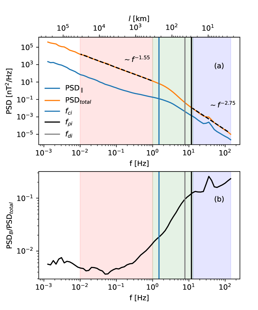
Figure 2: From top to bottom: magnetic field total spectrum $S_{total}$ in orange and magnetic field modulus spectrum computed with the parallel fluctuations spectrum $S_{\parallel}$ (Equation (5)) (a), and the ratio $S_{\parallel}/S_{total}$ (b). The vertical lines show the characteristic ion scales: ion cyclotron frequency $f_{ci}$ (in blue), and the frequencies computed with the Doppler shifted ion gyroradius $f_{\rho i}$ (in black) and the Doppler shifted ion inertial length $f_{di}$ (in grey). The frequency ranges are highlighted: MHD in red, ion scales in green and sub-ion scales in blue.

First we describe the spectral properties of the magnetic field. We apply wavelet transform with Morlet mother function (Torrence & Compo, 1998):

$$\psi_{0}(t)=\pi^{-1/4}e^{-t^{2}/2}e^{i\omega_{0}\,t},$$ (1)

where $\omega_{0}=6$ is the angular frequency of oscillations in the mother function (with normalized time). The wavelet transform of the magnetic field component $B_{i}(t)$ is defined as the convolution of $B_{i}(t)$ with scaled, translated and normalized $\psi_{0}(t)$ to have mother function $\psi$ with unit energy:

$$W[B_{i}](t,\tau)=\sum\limits_{n^{\prime}=0}^{N-1}B_{i}(t^{\prime})\psi^{\ast}[(t^{\prime}-t)/\tau]$$ (2)

where the sign ^∗ indicates complex conjugate.

Wavelet coefficients are influenced by the edge effects. Cone of influence (COI) curve separates the region of scales where edge effects become important as the function of time. To avoid this edge effect we consider a maximum scale equal to $\tau_{max}=10^{3}$ s. The intercept of $\tau_{max}$ with COI curve determines the time sub-interval $T^{\prime}=$ [00:22:49, 04:37:11] UT, where wavelet coefficients at the scales $\tau<\tau_{max}$ are negligibly influenced by the edge effect.

Figure 2(a), orange line, shows the total magnetic field power spectral density (PSD) $S_{total}(\tau)$, calculated using the time-averaging over the subinterval $T^{\prime}$ :

$$S_{total}(\tau)=\frac{2\delta t^{2}}{T^{\prime}}\sum\limits_{t\in T^{\prime}}\sum\limits_{i=R,T,N}|W[B_{i}](t,\tau)|^{2},$$ (3)

where $\delta t=0.008$ s is the time-step of the PSP merged magnetic field data. The relation between Fourier frequencies $f$ and time scales $\tau$ is $f\simeq 1/\tau$ for the Morlet wavelets with $\omega_{0}=6$. Figure 2(a), blue line, shows the PSD of compressive magnetic fluctuations. Compressive fluctuations are approximated here by the variation of magnetic field modulus. Indeed, this approximation is valid if the level of the fluctuations is significantly lower than the mean field $B_{0}$, i.e., $\delta B/B_{0}\ll 1$ (Perrone et al., 2016):

$$\delta(|B|^{2})=|\mathbf{B}_{0}+\delta\mathbf{B}|^{2}-|\mathbf{B}_{0}|^{2}\approx 2\delta B_{\parallel}B_{0}\approx\delta(B_{\parallel}^{2})$$ (4)

In the inertial range and at higher frequencies the condition $\delta B/B_{0}\ll 1$ is valid. So we calculate the parallel PSD, $S_{\parallel}(\tau)$, as it was done in Perrone et al. (2016):

$$S_{\parallel}(\tau)=\frac{2\delta t^{2}}{T^{\prime}}\sum\limits_{t\in T^{\prime}}|W[{|B|}](t,\tau)|^{2}$$ (5)

As we can see from Figure 2(a), $S_{total}(f)\sim f^{-1.55}$ within the inertial range $10^{-2}<f<1$ Hz, in agreement with Chen et al. (2020). Approaching ion kinetic scales, the spectrum steepens. The ion transition range, or simply ion scales, is present where the spectrum changes continuously its slope (Alexandrova et al., 2013; Kiyani et al., 2015). It is observed here nearly between the ion cyclotron frequency $f_{ci}=eB/2\pi m_{i}=1.4$ Hz and the frequency of the Doppler-shifted ion gyroradius $f_{\rho i}=V/2\pi\rho_{i}=11.4$ Hz. The frequency of the Doppler-shifted ion inertial length $f_{di}=V/2\pi d_{i}$ is in between these two frequencies. At $f>13$ Hz (sub-ion scales), the spectral index stabilizes at $-2.75$, in agreement with what is observed at 0.3 and 1 au between ion and electron scales (Alexandrova et al., 2009; Chen et al., 2010; Alexandrova et al., 2012, 2021).

Based on the magnetic field spectral properties and characteristic plasma scales ($f_{ci}$, $f_{\rho i}$ and $f_{di}$) we define the following frequency ranges $\Delta f_{j}$, shown as transparent color bands in Figure 2:

$$\Delta f_{j}=\begin{cases}(10^{-2},1)\text{ Hz}&\text{MHD inertial range}\;\text{(in red)}\\ (1,13)\text{ Hz}&\text{ion scales}\;\text{(in green)}\\ (13,128)\text{ Hz}&\text{sub-ion range}\;\text{(in blue)}\end{cases}$$ (6)

The corresponding timescale ranges $\tau_{j}$ will be used later in this article, and the index $j$ here and further in the article refers to one the following ranges:

$$\tau_{j}:\begin{cases}\tau_{MHD}=(100,1)\text{ s}&\\ \tau_{ion}=(1,0.08)\text{ s}&\\ \tau_{subion}=(0.08,0.008)\text{ s}&\end{cases}$$ (7)

The ratio of compressible fluctuations to the total power spectral density $S_{\parallel}/S_{total}$ is shown in Figure 2(b). In the inertial range, parallel magnetic fluctuations are much less energetic than perpendicular ones ($\delta B_{\|}\ll\delta B_{\perp}$), as is usually observed in the solar wind. At the sub-ion scales, the fraction of the parallel $S_{\parallel}(\tau)/S_{total}(\tau)$ increases, which is consistent with the results of Salem et al. (2012) at 1 au. The authors suggested that the observed spectral ratio can be explained by the presence of the kinetic Alfvén wave (KAW) cascade with nearly perpendicular wavevectors ($k_{\perp}\gg k_{\|}$). However, analyzing Cluster measurements (Lacombe et al., 2017) and 2D hybrid numerical simulation (Matteini et al., 2020) found that asymptotic compressibility value at sub-ion scales doesn’t match perfectly the KAW prediction. Finally, recent numerical simulations indicate that coherent structures, rather than waves, are energetically dominant on sub-ion scales (Papini et al., 2021).

4 Detection of coherent structures from MHD to sub-ion scales

In this section we describe the methodology to detect the structures from MHD down to sub-ion scales.

4.1 Local intermittency measure

Figure 3: A 30 minutes zoom, $[03:10,03:40]$ UT, within the analyzed time interval of 5 hours on November 6, 2018. From top to bottom: (a) magnetic field in RTN reference frame, (b) LIM of the magnetic fluctuations of the total energy $L(t,\tau)$ Equation (8), (c) artificial magnetic field $\mathbf{B}_{rand}$ with random phases and the same Fourier amplitudes as original magnetic field measurements, (d) LIM of the artificial signal $L_{rand}(t,\tau)$, (e) the comparison of the integrated LIMs $I(t)=\langle L(t,\tau)\rangle_{\tau\in[10^{-2},10^{3}]~{}s}$ (blue), and the $I_{rand}(t)=\langle L_{rand}(t,\tau)\rangle_{\tau\in[10^{-2},10^{3}]~{}s}$ (black). The horizontal red line shows $I_{threshold}=\text{max}(I_{rand}(t))$ as defined in Figure 4.

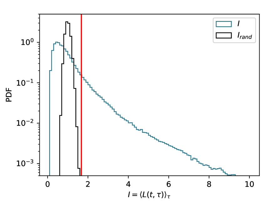
Figure 4: Histograms of the integrated LIM $I(t)$ and the random phased integrated LIM $I_{rand}(t)$. The threshold $I_{threshold}=\text{max}(I_{rand}(t))$ is shown by the red vertical line.

We use the Local Intermittency Measure (LIM) $L(t,\tau)$ (Farge, 1992) based on Morlet wavelets in order to detect the structures. The value $L(t,\tau)$ shows the total energy of fluctuations at a given moment in time $t$ at a given time scale $\tau$, relative to the average energy at that scale:

$$L(t,\tau)=\frac{\sum_{i=R,T,N}|W[B_{i}](t,\tau)|^{2}}{\langle\sum_{i=R,T,N}|W[B_{i}](t,\tau)|^{2}\rangle_{t\in T^{\prime}}}$$ (8)

where $T^{\prime}$ is the analyzed time interval.

In Figure 3 we show a 30 minutes zoom within $T^{\prime}$. Panel (a) gives RTN components of the measured $\mathbf{B}$. Panel (b) shows the observed $L(t,\tau)$. The vertical elongations of enhanced $L(t,\tau)$ values are due to coupled (or coherent) phases of the fluctuations (Lion et al., 2016; Perrone et al., 2016; Alexandrova, 2020). Indeed, to see this point better, we construct an artificial signal that has the same Fourier spectrum as the original magnetic field measurements, but with random phases (Hada et al., 2003; Koga & Hada, 2003). This synthetic signal $\mathbf{B}_{rand}$ is shown in Figure 3(c), while the corresponding LIM $L_{rand}(t,\tau)$ is shown in the panel (d). The energy distribution of the synthetic signal is incoherent (randomly distributed in the $(t,\tau$)–plane), i.e., peaks of $L_{rand}(t,\tau)$ at different $\tau$ are not observed at the same time. Therefore, the vertical elongations in the observed $L(t,\tau)$ correspond to magnetic fluctuations with coupled phases across scales where the elongation is observed. The high energy of these events with respect to the mean is a sign of intense coherent structures formed in the turbulent medium (e.g. Farge, 1992; Bruno, 2019). So, we observe coherent structures which extend from inertial to sub-ion timescales. Using the Taylor hypothesis, the timescale range $\tau\in\tau_{all}=[10^{-2},10^{3}]$ s can be converted into the spatial range $\ell=V\cdot\tau\in[3,3\cdot 10^{5}]$ km.

The difference between random-phased signal and original magnetic field data suggests a methodology for detecting the central times of coherent structures. Specifically, we integrate LIM over the timescale range $\tau_{all}=[10^{-2},10^{3}]$ s:

$$I(t)=\int_{\tau\in\tau_{all}}L(t,\tau)\,d\tau$$ (9)

Figure 3(e) shows $I(t)$ (blue line), random phased integrated LIM $I_{rand}(t)$ (black line) and the threshold $I_{threshold}=\text{max}(I_{rand}(t))$ (red horizontal line). The local maxima of $I(t)>I_{threshold}$ give the central times of the coherent structures present in the original signal. We refer below this method as the integrated LIM selection.

The comparison of original $I(t)$ and random phased $I_{rand}(t)$ distributions is shown on Figure 4. The $I_{rand}$ distribution (in black) is close to Gaussian with a mean of 1 (because of the normalization and random phases). On the contrary, $I(t)$ (in blue-azure) has a long tail of extreme values due to the presence of coherent structures integrated over all time scales.

The integrated LIM selection does not have a predetermined scale at which the structure is searched for but it is preferentially focused on scales where the vertical enhancements in the LIM $L(t,\tau)$ are observed. Applying it on $T^{\prime}=$[00:22:49,04:37:11] on 6 November 2018, we find $N=9485$ structures. If we define the filling factor of the structures as the normalized total time duration where the integrated LIM is over the threshold:

$$P=\text{Time}(I(t)>I_{threshold})/T^{\prime},$$

we find that the structures cover $14\%$ of the analyzed time interval $T^{\prime}$.

In this paper, we will also use the integrated LIM over the reduced time-scale ranges, to understand in more details the nature of the structures at MHD, ion and subion scales, where physics is different. So, we can define integrated LIM $I_{i}=(I_{MHD},I_{ion},I_{subion})$ over the corresponding range of timescales $\tau_{j}=(\tau_{MHD},\tau_{ion},\tau_{subion})$, defined in Equation (6):

$$I_{j}(t)=\int_{\tau\in\tau_{j}}L(t,\tau)\,d\tau$$ (10)

Similarly, integrating $L_{rand}(t,\tau)$ over $\tau_{j}$ we define random phased integrated LIM $I_{rand,j}(t)$. Thus, we can find the central times of the structures within these scale-bands as the times of the local maxima for $I_{j}(t)>I_{threshold,j}=\text{max}(I_{rand,j}(t))$.

This band-integrated LIM selection allows us to see how the number of the structures $N$ and filling factor $P$ changes with scale band. We find a relatively small number of MHD scale structures ($N_{MHD}=$196) with high filling factor ($P=$12%), compared to $P=$7% and $P=$6% for much more numerous ion scale structures ($N_{ion}=2028$) and sub-ion scale structures ($N_{sub-ion}=11167$). We remark, that our estimations of $P$ are conservative, as far as only time where LIM is over the threshold is counted, but the structure’s field decreasing from its center exist outside of the time where the energy of the structure is concentrated. So, the filling factor can be more than twice larger than given here. Finally, numerous small scale events populate larger ones and may exist outside them as well.

4.2 Magnetic field at different scales

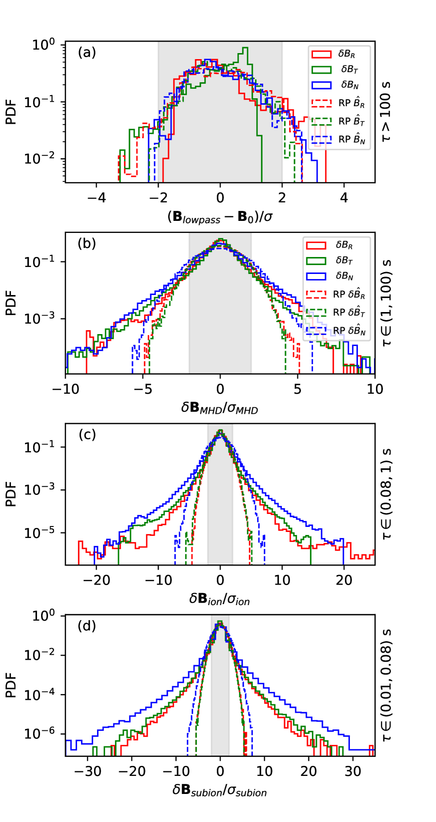
Figure 5: Histograms of magnetic field fluctuations (solid) compared to the signal with random phases (RP, dashed). The first panel from the top shows the centered lowpass-filtered fluctuations of the magnetic field. Panels (b-d) show bandpass-filtered fluctuations on MHD inertial, ion kinetic, and sub-ion scales, respectively. The horizontal axis is normalized to the standard deviation of the random-phased signal. The area within two standard deviations of the random-phased signal is highlighted in gray.

	$\sigma_{R}$	$\sigma_{T}$	$\sigma_{N}$	$\sigma_{noise}$	$s_{R}$	$s_{T}$	$s_{N}$	$\langle|s|\rangle$	$\kappa_{R}$	$\kappa_{T}$	$\kappa_{N}$	$\langle\kappa\rangle$
Low-pass	37	31	35	-	1.1	-1.1	0.5	0.9	3.8	3.8	3.1	3.6
MHD	9	8.6	11	7.8	0.2	-0.5	0.01	0.2	7.7	8.7	6.5	7.6
Ion scales	1.5	1.6	2.2	1.55	0.1	-0.2	-0.01	0.1	16.3	14.0	10.8	13
Sub-ion	0.12	0.12	0.15	0.11	0.01	-0.01	-0.04	0.02	11.6	19.3	24.4	18

Table 1: Main parameters of the distributions shown in Figure 4 for the magnetic field components in RTN coordinates. From left to right: standard deviation $\sigma_{RTN}$ [nT], average standard deviation $\sigma_{noise}$ [nT] (in absence of coherent structures), skewness $s_{RTN}$, average absolute skewness $\langle|s|\rangle$, kurtosis $\kappa_{RTN}$, and the average kurtosis $\langle\kappa\rangle$.

Thanks to Morlet wavelets and LIM we know now the central times of the structures covering all scales and the ones within different scale bands. In order to study magnetic field fluctuations $\delta\mathbf{B}$ in the physical space around these central times, within different scale bands, we use band-pass filter for fluctuations on frequency ranges given by Equation (6) and shown by color bands in Figure 2. We complete this analysis by studying the large scale fluctuations of $\mathbf{B}_{lowpass}-\mathbf{B}_{0}$ where the mean field $\mathbf{B}_{0}$ is defined as the average field over the time interval $T^{\prime}$. We use finite impulse response (FIR) Humming low-pass filter with a cut-off frequency of $10^{-2}$ Hz to calculate the large scale magnetic field fluctuations of $\delta\mathbf{B}=\mathbf{B}_{lowpass}-\mathbf{B}_{0}$.

Figure 5 shows distributions of the filtered magnetic field (solid lines) compared to the filtered signal with random phases (dashed lines). Panel (a) shows the lowpass-filtered fluctuations of the magnetic field. Panels (b-d) show bandpass-filtered fluctuations on MHD, ion, and sub-ion scales, respectively. At each band of scales we characterise the amplitude of incoherent fluctuations as follows:

$$\sigma_{noise,j}=\text{std}(\delta B_{j}(t\in T_{\text{no struct}}))$$ (11)

where $T_{\text{no struct}}=\text{Time}(I_{j}(t)<I_{threshold,j})$. The gray area in panels (b-d) is bounded by $\delta\mathbf{B}_{rand,j}/\sigma_{noise,j}=\pm 2$.

The random phase signal fluctuations have Gaussian distributions at all scales (Figure 5). The observed $\delta\mathbf{B}$ show scale-dependent deviation from Gaussianity. Table 1 gives the moments of the observed distributions for 3 components and at 4 different scale ranges. The distributions have non-zero skewness $s$ (a normalized measure of a distribution asymmetry). The fourth normalized moment, kurtosis $\kappa$, increases from 3-4 at large scales, up to 12-24 at sub-ion scales. In comparison, Gaussian noise has $s=0$ and $\kappa=3$.

Distributions of lowpass magnetic field components are asymmetric with respect to zero, especially radial and tangential (see Figure 5(a)). The skewness of those components has high absolute value and opposite signs: $s_{R}=1.1$ and $s_{T}=-1.1$. The lowpass magnetic field distributions doesn’t have pronounced non-gaussian tails, so the kurtosis $\kappa$ are slightly above 3, so close to the gaussian noise value (see Table 1)).

In the inertial and smaller scale ranges, the distributions have weaker asymmetry ($\langle|s|\rangle=(|s_{R}|+|s_{T}|+|s_{N}|)/3\leq 0.2$). Non-gaussian tails are identified at MHD scales (Figure 5(b)) and become even more pronounced at ion and sub-ion scales (Figure 5(c-d)). The kurtosis $\kappa_{T}$ and $\kappa_{N}$ monotonically increase from MHD to subion scales (see Table 1). The kurtosis of the radial magnetic field $\kappa_{R}$ component is growing from MHD to ion scales and then decrease at subion scales. This behavior of $\kappa_{R}$ can be explained by the proximity of the SCM noise, which starts to influence $\delta B_{R,subion}$, the weakest of the 3 components of magnetic fluctuations at these scales, see Figure 5(d).

5 Model structures

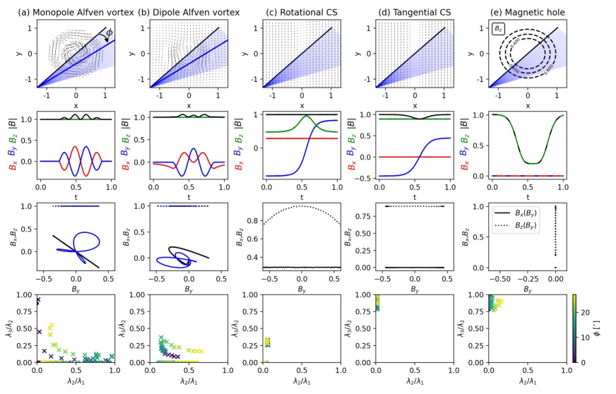
Figure 6: Simulation of the spacecraft crossing (a) a monopole Alfvén vortex, (b) a dipole vortex, (c) a rotational and (d) a tangential discontinuities, and (e) a magnetic hole. The first row shows the magnetic field vector in the plane perpendicular to the background magnetic field. The sector, shown in blue, is a set of trajectories crossing the structure at different angles in order to collect statistics of MVA eigenvalues. The panels in the second line show the magnetic field in the MVA frame of reference, which would be measured by the spacecraft when it crosses the structure along the black trajectory. Panels in the third line show the hodograph - indicating polarisation for off-center (blue) and central (black) trajectories. The bottom row shows the eigenvalue ratios for the set of trajectories shown within the blue cone in the first row in the presence of noise, with $\epsilon=0.001$ (circles) and $\epsilon=0.1$ (crosses). The trajectory angle $\phi$, defined in the top left panel, is coded with colors (see the color scale at the right bottom). Each dashed line shows the boundary of the regions on the eigenvalue ratios plane that is consistent with crossing the given model of structures in the presence of the noise level $\epsilon\in(0,0.1)$.

We consider here several theoretical models of the structures we think we cross by PSP at different scales. This will give us a background for the interpretation of the observed events detected with the method described above. The models we describe here have been developed in the MHD framework. We will use them at kinetic scales as well from the topological point of view only. The trajectory of a spacecraft across a structure matters for the polarization and the amplitude anisotropy. That is why we will explore the polarization and the Minimum Variance Analysis (MVA, Sonnerup & Scheible, 1998) results as a function of the spacecraft trajectory across the model structures.

5.1 Alfvén vortices

Alfvén vortices are cylindrically symmetric coherent structures that were introduced by Petviashvili & Pokhotelov (1992). The model is based on the reduced MHD equations (Kadomtsev & Pogutse, 1974; Strauss, 1976), where the principal assumptions are the perpendicular anisotropy in the wave-vector space, $k_{\perp}>>k_{\parallel}$, and slow time variations. Two main types of vortices are distinguished: monopolar and dipolar.

5.1.1 Monopole Alfvén vortex

Let the axis $z$ be along the background magnetic field $\mathbf{B}_{0}$. The transverse magnetic field $\delta\mathbf{B}_{\perp}=\nabla A_{z}\times\mathbf{z}$ and velocity $\delta\mathbf{V}_{\perp}=\mathbf{z}\times\nabla\psi$ perturbations are expressed with the axial component of the vector potential $A_{z}$ and the velocity flux function $\psi$. The model assumes linear proportionality $\psi=\xi A_{z}$, or equivalently $\delta\mathbf{V}_{\perp}/V_{A}=\xi\,\delta\mathbf{B}_{\perp}/B_{0}$ (generalised Alfvén relation).

A monopole Alfvén vortex is localized within the cylinder of the radius $a$, and the cylinder is aligned with $\mathbf{B}_{0}$. The model assumes that the total current inside $r<a$ is zero. If $\delta\mathbf{B}_{\perp}$ is continuous at $r=a$, it implies the condition $J_{1}(ka)=0$, where $J_{1}$ is the first order Bessel function. This defines the parameter $k$ for a given radius $a$. The monopole vortex solution writes (in dimentionless units, see Petviashvili & Pokhotelov (1992)):

$$\begin{cases}A_{z}=A_{0}\,(J_{0}(kr)-J_{0}(ka)),&r<a\\ A_{z}=0,&r>a\end{cases}$$ (12)

where $A_{0}$ is the monopole vortex amplitude and $J_{0}$ is the zero order Bessel function.

A monopole Alfvén vortex in the plane perpendicular to its axis is shown on the top left panel of the Figure 6. The amplitude of the structure, $\delta B_{\perp}/B_{0}=0.5$, is taken to be comparable to the observations (see Figure 9(b)).

Spacecraft measurements depend on the trajectory along which the vortex is crossed. The set of trajectories, selected to cross the vortex, is shown by the blue transparent cone on the top left panel of Figure 6. The set is parametrised by the angle $\phi$. Two trajectories, central ($\phi=0^{\circ}$) and off-center ($\phi=10^{\circ}$), are shown in black and blue lines correspondingly. The second panel from the top shows the three magnetic field components of the monopolar vortex crossed by a spacecraft along the black trajectory in the top panel. The third panel shows the dependencies $B_{x}(B_{y})$ and $B_{z}(B_{y})$ for both central and off-center trajectories (black and blue lines respectively). The off-center trajectory has ’clover’-like polarisation in $B_{x}(B_{y})$ (blue curve). In case of the crossing through the center, the polarisation is linear (black line).

Figure 6 (column (a), bottom row) shows the MVA eigen-value ratio $\lambda_{3}/\lambda_{2}$ as a function of $\lambda_{2}/\lambda_{1}$ for 50 different trajectories (see the blue cone in the top panel). The eigen-values are ordered as $\lambda_{1}>\lambda_{2}>\lambda_{3}$, with the eigen-vector $\mathbf{e_{3}}$ beeing the minimum variance direction. The color between violet and yellow indicates the angle $\phi$ of the trajectories: $\phi=0^{\circ}$ corresponds to the crossing through the center and $\phi=25^{\circ}$, to the side-crossing. In this plot we test the effect of an added noise with a relative amplitude $\epsilon$ defined by

$$\epsilon=\delta B_{noise}/\delta B_{\perp}$$ (13)

where $\delta B_{noise}$ is the noise amplitude and $\delta B_{\perp}$ is the amplitude of the vortex. The eigenvalue ratios $\lambda_{2}/\lambda_{1}$ and $\lambda_{3}/\lambda_{2}$ are dependent on $\epsilon$. Two levels of noise are shown: $\epsilon_{1}=0.001$ with filled circles, and $\epsilon_{2}=0.1$ with crosses. In case of negligible noise, the points are located along the x-axis. For larger $\epsilon$, the eigenvalues become more comparable (they are identical for a noise dominated case), then the points move toward the upper right corner on the plane $(\lambda_{2}/\lambda_{1},\lambda_{3}/\lambda_{2})$. The $\epsilon$ estimation from observations is discussed further in Section 7.

For the majority of trajectories, except central ($\phi<3^{\circ}$) and extreme-off-center/tangential ones ($\phi>22^{\circ}$), the minimum variance direction $\mathbf{e}_{3}$ is well-defined ($\lambda_{3}/\lambda_{2}\sim 0$) and it is parallel to the axis of the vortex. Indeed, the vortex model describes $\delta B_{\perp}$ and assumes $\delta B_{z}=0$. So, in observations, $\mathbf{e}_{3}$ (when it is well-defined) is a good approximation for the vortex axis. As far as the vortex cylinder is field-aligned, the angle between $\mathbf{e}_{3}$ and $\mathbf{B}_{0}$ must be small, $\theta_{B_{0},3}\sim 0^{\circ}$.

In case of the central crossing ($\phi<3^{\circ}$), only $\mathbf{e}_{1}$ is well-defined, because $\lambda_{2}/\lambda_{1}\sim 0$, $\lambda_{3}/\lambda_{2}\sim 1$. In this case the eigenvector of maximal variance $\mathbf{e}_{1}$ is perpendicular to the crossing trajectory $\mathbf{e}_{1}\perp\mathbf{V}$ and to the background magnetic field $\mathbf{e}_{1}\perp\mathbf{B}_{0}$. Therefore, $\theta_{V,1}\sim 90^{\circ}$ and $\theta_{B,1}\sim 90^{\circ}$ are expected in observations.

In addition, for the vortex to be observable, the spacecraft must cross it along a trajectory inclined at a sufficient angle relative to the vortex axis, so $\theta_{B,V}\neq 0^{\circ}$ and $\theta_{V,3}\neq 0^{\circ}$ (if $\mathbf{e}_{3}$ is well-defined).

5.1.2 Dipole Alfvén vortex

As in case of the monopole vortex, the dipole vortex is a coherent structure localised inside the cylinder of the radius $a$ and the generalised Alfvén relation $\delta\mathbf{V}_{\perp}/V_{A}=\xi\,\delta\mathbf{B}_{\perp}/B_{0}$ is assumed.

The particular property of the dipole Alfvén vortex model is that it’s axis can be inclined by a small angle $\theta$ with respect to the background magnetic field $B_{z}=B_{0}$. We define $\alpha=\tan(\theta)$. Without restriction of generality, let the axis of the vortex be in the $(y,z)$-plane. If $\theta\neq 0$, the dipole vortex propagate along $y$ at the speed $u\propto\alpha$. The continuity of $\delta\mathbf{B}_{\perp}$ at $r=a$ requires that the amplitude of the dipole vortex is not arbitrary, but defined by $\alpha$ and $k$. In the reference frame moving with the vortex, the dimentionless vector potential of the dipole vortex is (Petviashvili & Pokhotelov, 1992; Alexandrova, 2008):

$$\begin{cases}A_{z}=\frac{-2\alpha}{kJ_{0}(ka)}\,J_{1}(kr)\frac{x}{r}+\alpha\,x,&r<a\\ A_{z}=\alpha x\frac{a^{2}}{r^{2}},&r>a\end{cases}$$ (14)

Figure 6 column (b) shows the magnetic field of the dipole vortex in the $(x,y)$-plane and trajectories of synthetic spacecraft across it, in the same format as for the monopole vortex (column (a)). The magnetic field components are symmetric in time around the vortex axis (while for the monopole vortex they are anti-symmetric). The magnetic polarisation (third panel from the top) is different for the crossing at the vortex center (black trajectory) and the side crossing (blue trajectory).

Figure 6(column (b), bottom panel) gives the minimal variance eigenvalues ratios for two noise levels. In case of the low noise, $\epsilon=0.001$, $\lambda_{3}/\lambda_{2}\sim 0$ and $\lambda_{2}/\lambda_{1}\in[0.1,0.6]$ (filled circles). For $\epsilon=0.1$, as for the monopole vortex, both ratios increase: the points in the $(\lambda_{3}/\lambda_{2},\lambda_{2}/\lambda_{1})$–plane move towards the upper right corner.

The magnetic fluctuations of the dipole vortex are transverse, so the minimum variance direction $\mathbf{e}_{3}$ (when it is well-defined) is along the axis of the vortex $\mathbf{z}$. The angle between $\mathbf{e}_{3}$ and $\mathbf{B}_{0}$ is expected to be small $\theta_{B_{0},3}\sim 0^{\circ}$ according to the assumption of the model. Maximum and intermediate MVA eigenvectors $\mathbf{e}_{1}$, $\mathbf{e}_{2}$ lie in the plane perpendicular to $B_{0}$.

5.2 Current sheets

Current sheets are planar coherent structures that separate the plasma with different magnetic field directions. Current sheets with large rotation angles across the sheet represent the boundaries of magnetic tubes, according to Bruno et al. (2001); Borovsky (2008). The population of current sheets with smaller rotation angles is much more numerous (Borovsky, 2008). They might be formed spontaneously as a result of the turbulent cascade, (e.g., Veltri, 1999; Mangeney, 2001; Servidio et al., 2008; Salem et al., 2009; Zhdankin et al., 2012; Greco et al., 2008, 2009, 2012).

MHD classification of current sheets include rotational (RDs) and tangential (TDs) discontinuities (e.g., Baumjohann & Treumann, 1997; Tsurutani et al., 2011). A typical method to distinguish RD from TD is based on the normalised change in magnetic field magnitude $\Delta B/B$ across the discontinuity (which is zero for RD) and the normal magnetic field component $B_{n}/B$ (which is zero for TD). However, observations showed that current sheets can combine both properties of RTs and TDs (e.g., Neugebauer, 2006; Artemyev et al., 2019).

5.2.1 Rotational discontinuity

RDs are characterised by the correlated rotation of magnetic field and velocity (Walen relation in case of the pressure isotropy: $\mathbf{\delta B}/B_{0}=\pm\mathbf{\delta V}/V_{A}$), constant magnetic and plasma pressures across the sheet ($\Delta B/B=\Delta P/P=0$). Plasma on the both sides of a RD is magnetically connected, i.e. $B_{n}\neq 0$.

Let the normal to the current sheet $\mathbf{n}$ be along $\mathbf{e}_{x}$, $B_{n}$ and $B_{t}$ denote normal and tangential magnetic field components. The condition $\mathbf{\nabla}\cdot\mathbf{B}=0$ implies $B_{x}=B_{n}=\text{constant}$. We use the same rotational discontinuity model as in Goodrich & Cargill (1991), where the magnetic field rotates smoothly by an angle $\zeta(x/\ell)=\Delta\zeta/2\tanh(x/\ell)$ with a total angle $\Delta\zeta$ across the RD with thickness $\ell$:

$$\begin{cases}B_{x}(x)=B_{n}\\ B_{y}(x)=B_{t}\cos(\zeta(x/\ell))\\ B_{z}(x)=B_{t}\sin(\zeta(x/\ell))\end{cases}$$ (15)

We select $\Delta\zeta=120^{\circ}$ as in the example that we discuss in Section 6.3. According to the statistical study of the current sheets from the first PSP perihelion, thin current sheets have smaller magnetic field rotation angles $\Delta\zeta\sim 21^{\circ}\times(\ell/d_{i})^{0.32}$, where $\ell$ is the CS thickness and $d_{i}$ is the proton inertial length (Lotekar et al., 2022). For rotational discontinuities with smaller $\Delta\zeta$ the polarization becomes closer to linear, i.e., closer to case of tangential discontinuity model discussed in the Section 5.2.2. In terms of eigenvalues, $\lambda_{3}/\lambda_{2}$ increases while $\Delta\zeta$ decreases. The selection of $\Delta\zeta=120^{\circ}$ corresponds to strong RDs. The other ones cannot be distinguished from TDs with the polarisation and MVA eigenvalue ratios.

We show crossings of this RD model by a synthetic spacecraft in Figure 6 column (c). Rotational discontinuity has an arch-like hodograph (Figure 6, column (c), third row). Discontinuities with arch-shaped hodograph have been previously observed in the solar wind (Neugebauer, 1989; Riley et al., 1996; Tsurutani et al., 1996; Sonnerup et al., 2010; Haaland et al., 2012; Paschmann et al., 2013). In the bottom panel, both ratios $\lambda_{2}/\lambda_{1}\simeq\lambda_{3}/\lambda_{2}\simeq 0$ when the noise level is low (see dots). For higher noise, $\lambda_{3}/\lambda_{2}$ increases more than $\lambda_{2}/\lambda_{1}$ (see crosses).

If the noise level is small enough, so that the MVA eigenvectors $(\mathbf{e}_{1},\mathbf{e}_{2},\mathbf{e}_{3})$ are well-defined, they coincide with the basis vectors $(\mathbf{z},\mathbf{y},\mathbf{x})$ of the reference frame of the sheet (for any crossing trajectory).

5.2.2 Tangential discontinuity

TDs separate two magnetically disconnected regions of plasma, so normal magnetic field component $B_{x}=B_{n}=0$. We use the Harris-like current sheet model, with a constant guide field $B_{z}=B_{0}$ (Harris (1962)):

$$\begin{cases}B_{x}=0\\ B_{y}=B_{t}\tanh(x/\ell)\\ B_{z}=B_{0}\end{cases}$$ (16)

In presence of the strong guide field $B_{0}\gg B_{t}$, the current density is quasi-parallel to magnetic field. So, the current sheet is quasi-force-free in accordance with what was found in observations (Artemyev et al., 2019).

Crossing of tangential discontinuity is shown in Figure 6 in column (d). The polarisation is linear, $\lambda_{2}/\lambda_{1}\sim 0$, $\lambda_{3}/\lambda_{2}\sim 1$. Only the maximum MVA eigenvector is unambiguously defined: $\mathbf{e}_{1}=\mathbf{y}$. The $\mathbf{e}_{2}$ and $\mathbf{e}_{3}$ are in $x-z$ plane, but $\mathbf{e}_{3}$ is not obligatory directed along the normal to the sheet $\mathbf{x}$. The degree of compressibility $\delta B_{\parallel}/B_{t}\neq 0$ where $\delta B_{\|}$ is the variation along $\mathbf{B}_{0}$.

5.3 Magnetic holes

Magnetic hole represents a localized magnetic field modulus decrease. MHD-scale magnetic holes (with crossection widths ranging from $\sim 10\,\rho_{p}$ to $\sim 10^{3}\rho_{p}$, where $\rho_{p}$ is the proton Larmor radius), are quite rare events: at 1 AU the occurrence rate of 0.6 per day was observed by Stevens & Kasper (2007). Closer to the Sun the occurrence rate was found to be higher: from 2.4 per day at 0.7 AU to 3.4 per day at 0.3 AU (Volwerk et al., 2020).

MMS solar wind observations (Wang et al., 2020) and kinetic simulations (Roytershteyn et al., 2015; Haynes et al., 2015) have found magnetic holes at sub-ion scales. PIC simulations show that magnetic holes (defined as regions of magnetic field depression) tend to have cylindrical field-aligned geometry (Roytershteyn et al., 2015; Haynes et al., 2015).

We consider the magnetic hole model where the magnetic field direction does not change across the structure (linear magnetic hole). We suppose that the hole has cylindrical geometry and the axis is along $\mathbf{e}_{z}$. The radius of the hole is designated as $a$.

$$\begin{cases}B_{x}=0\\ B_{y}=0\\ B_{z}=B_{0}-\delta B_{\parallel}/\cosh\left((x/a)^{2}+(y/a)^{2}\right)\end{cases}$$ (17)

The magnetic hole crossing is shown on column (e) of the Figure 6. Magnetic hole has linear polarisation, $\lambda_{2}/\lambda_{1}\sim 0$, $\lambda_{3}/\lambda_{2}\sim 1$ and the magnetic perturbation is parallel $\delta\mathbf{B}=\delta\mathbf{B}_{\parallel}=\delta B_{\parallel}\mathbf{e}_{\parallel}$.

6 Examples of structures

We consider coherent structures detected by the integrated LIM over all scales and above the threshold, $I>I_{threshold}$ (see Section 4.1). Among nearly $\sim 10^{4}$ events we have selected 374 with $I/I_{threshold}\geq 6$ for visual examination. All of them have a localised event at sub-ion scales, which is embedded in a larger event at ion scales. At its turn, this ion scale event is embedded in an MHD scale event. Here we show 3 such examples of Russian dolls with different types of the structures at different scales, found among the subset of 374 events.

For each event, we consider the raw data during 200 seconds around the central time, then we consider filtered magnetic field data $\delta B_{j}$ at time scales defined by equation (7), with $j=$‘MHD’, ‘ion’ and ‘subion’. The duration of each signal is defined by the largest time scale in each time-range, i.e., $\pm$100 s, $\pm$1 s and $\pm$0.08 s , respectively. Then, we consider corresponding polarization of magnetic field. Finally, we examine plasma parameters for 200 s around central times.

6.1 Example 1

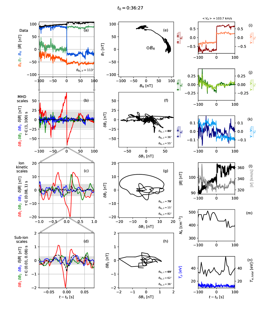
Figure 7: Example 1: A tangential discontinuity on MHD scales. The four panels on the left represent magnetic fluctuations near the central time $t_{0}$ = 0:36:27 UT. (a) Original magnetic field in RTN reference frame, (b) bandpass filtered magnetic fluctuations at MHD, (c) ion and (d) sub-ion frequency ranges, see equations 6 and 7 in local MVA reference frame. (e-h) Corresponding polarisation plots. The orientation of MVA basis vectors $\{\mathbf{e}_{i}\}_{i=1,2,3}$, with respect to the background magnetic field $\mathbf{B}_{0}$ is provided in the legend with $\theta_{B_{0},i}$ angles. Angles for well-defined MVA basis vectors are shown in bold. Panels of the right column show different plasma parameters at MHD scales: (i-k) the correlation between $(\mathbf{B}-\langle\mathbf{B}\rangle)/B_{0}$ and $(\mathbf{V}-\langle\mathbf{V}\rangle)/V_{A}$, (l) the magnetic field and velocity modulus ($|B|$ and $|V|$), (m) the electron density $N_{e}$, (n) proton and electron temperatures $T_{p}$, $T_{e,total}$.

The first event was observed on November 6, 2018, at $t_{0}=$00:36:27 UT. Figure 7(a) shows magnetic field data in the RTN reference frame during 200 s around $t_{0}$. Here, $B_{T}$ and $B_{N}$ components change sign in the center, magnetic field rotates by the angle $\Delta\zeta=80^{\circ}$. Thus, this is an example of a current sheet. The flow-to-field angle is $\Theta_{BV}=113^{\circ}$, so the PSP cross this structure under a quasi-perpendicular angle. The polarization of these fluctuations in the plane $(B_{N},B_{T})$ is shown in panel (e). The out of plane $B_{R}$ is negative and nearly constant during the considered time interval, so this discontinuity is not at the edge of a switchback.

Figure 7(b) shows band-pass filtered MHD inertial range magnetic fluctuations $\delta\mathbf{B}_{MHD}$ during the same 200 s around $t_{0}$ in the MVA reference frame. The grey horizontal bands indicates $\pm 2\sigma_{MHD}$ (two standard deviations of the random phase signal at MHD scales). The discontinuity in the center is due to the presence of the current sheet detected already in the raw data with the amplitude $\delta B/B\simeq 1.4$. The shape of $\delta B_{1}$ (red line) around $t_{0}$ is due to the band-pass filtering or a current sheet shown above in panel (a). The corresponding polarization (panel (f)) is nearly linear. In the legend, we indicate the angles between the corresponding mean field $\mathbf{B}_{0}$ and the MVA basis. The MVA basis vectors $\mathbf{e}_{1}$, $\mathbf{e}_{2}$ and $\mathbf{e}_{3}$ are well-defined if both eigenvalue ratios are small, $\lambda_{2}/\lambda_{1}<0.3$ and $\lambda_{3}/\lambda_{2}<0.3$ (Paschmann & Daly, 1998). If only the first (second) of the ratios is below $0.3$, then only $\mathbf{e}_{1}$ ($\mathbf{e}_{3}$) is unambiguously defined. The angles with eigenvalue ratios below $0.3$ are shown in bold in the legend of the polarizaion plane. So, one can see a linear polarization, with the maximum variance direction $\mathbf{e_{1}}$ quasi-perpendicular to $\mathbf{B}_{0}$, $\Theta_{B,1}=80^{\circ}$. The intermediate $\mathbf{e}_{2}$ and minimum $\mathbf{e}_{3}$ variance directions are ill defined.

Figure 7(c) shows a zoom to the time interval of $\pm 1$ s around the same central time $t_{0}$. The grey horizontal band indicates $\pm 2\sigma_{ion}$. For ion scales, the amplitude is significant, $\delta\mathbf{B}_{ion}/B_{0}\sim 0.2$, but smaller then one. The shape of $\delta\mathbf{B}_{ion}$ is not the filtering remnant of the current sheet, as shown in the Appendix. The black dashed line shows the fluctuations of magnetic field modulus $\delta|B|$, which are negligible. Here, the local MVA frame is well defined and minimal and maximal variations are perpendicular to the field. The elliptic polarization and the shape of magnetic fluctuations at ion scales resemble the crossing of a dipole vortex (shown in the Figure 6(b)). Thus, we observe a vortex like structure embedded in the current sheet.

Figure 7(d) shows the zoom-in to the time interval of $\pm 0.07$ s around $t_{0}$. The grey horizontal band indicates $\pm 2\sigma_{sub-ion}$. Here magnetic fluctuations $\delta\mathbf{B}_{sub-ion}$ are well localized in time and has a non-negligible fluctuations of the modulus of magnetic field $\delta|B|/\delta B_{1}=0.4$ (black dashed line). Observation of an important compressible component in $\delta\mathbf{B}_{sub-ion}$ is in agreement with a statistical increase of compressibility at sub-ion scale (see the spectrum of compressible fluctuations, Figure 2(b)). Sub-ion scale fluctuations have elliptic polarisation. The maximum MVA eigenvector is quasi-perpendicular to the background magnetic field $\theta_{B_{0},1}=69^{\circ}$. The properties mentioned above can be explained as the crossing of a compressible vortex through its center (Jovanović et al., 2015).

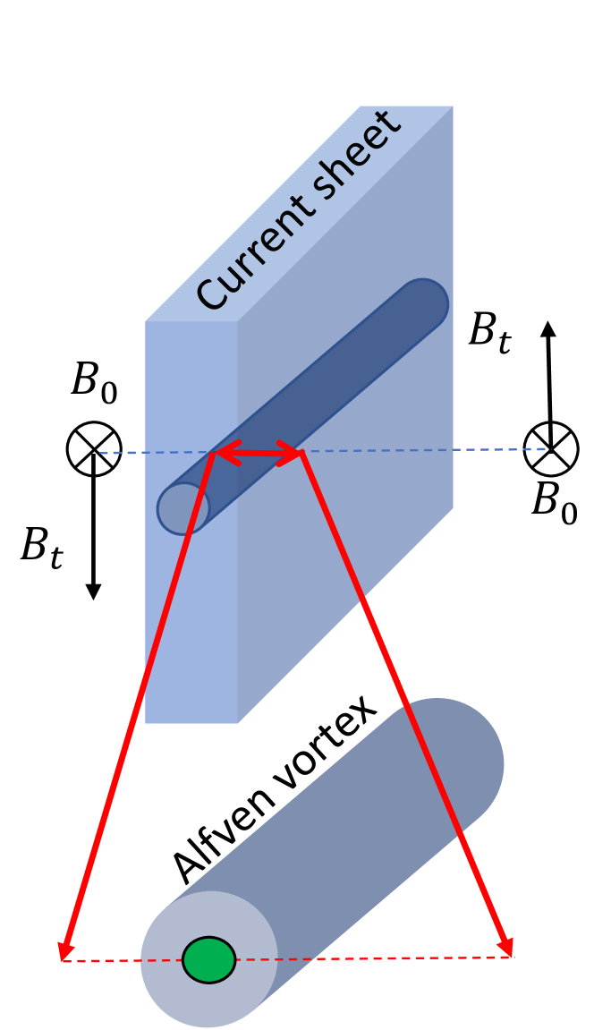
Figure 8: Schematic sketch of the Example 1, shown in the Figure 7. The blue dashed line illustrates the crossing trajectory. The mean magnetic field ($B_{0}$) and the tangential ($B_{t}$) component are shown in black on both sides of the current sheet. The red lines indicate the zoom to the embedded ion-scale vortex. A compressible sub-ion scale vortex is shown in green. The embedded sub-structures are shown not to scale.

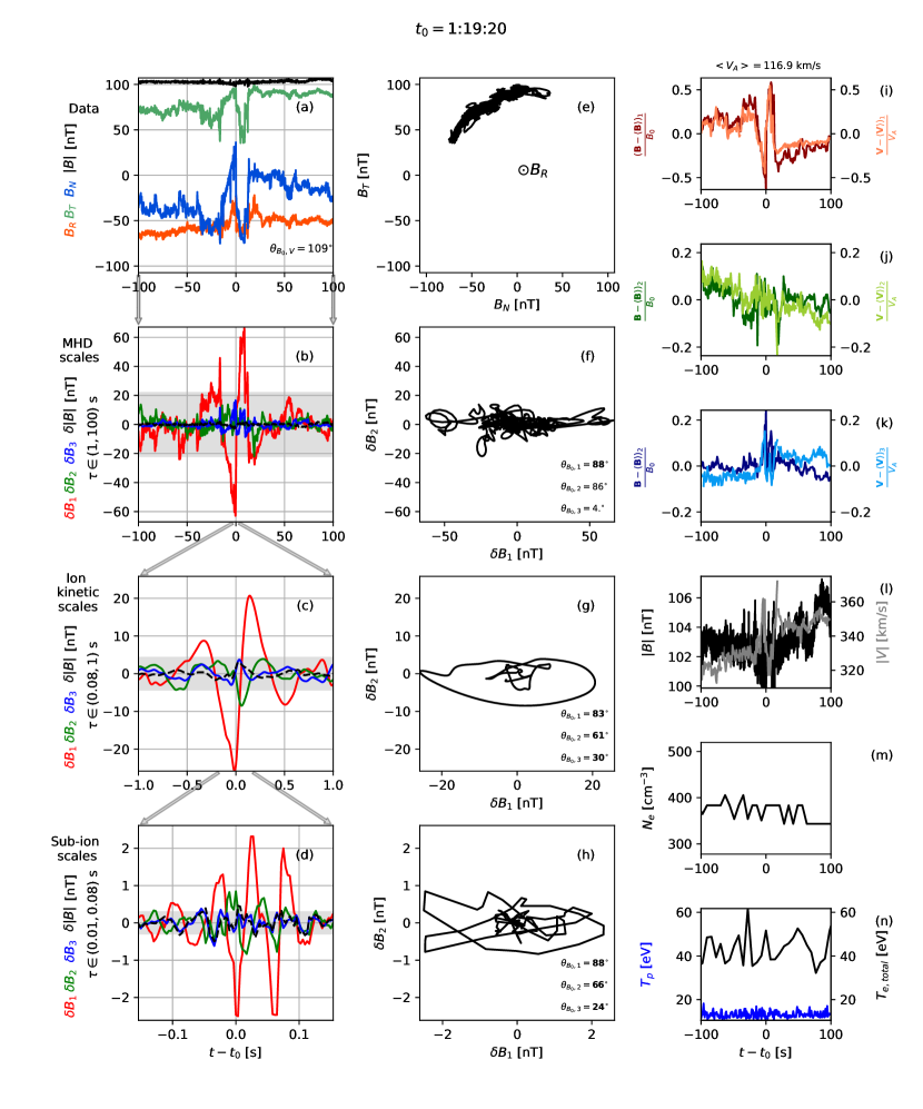
Figure 9: Example 2: An Alfvén vortex embedded in a week current sheet on MHD scales. The format is the same as Figure 7.

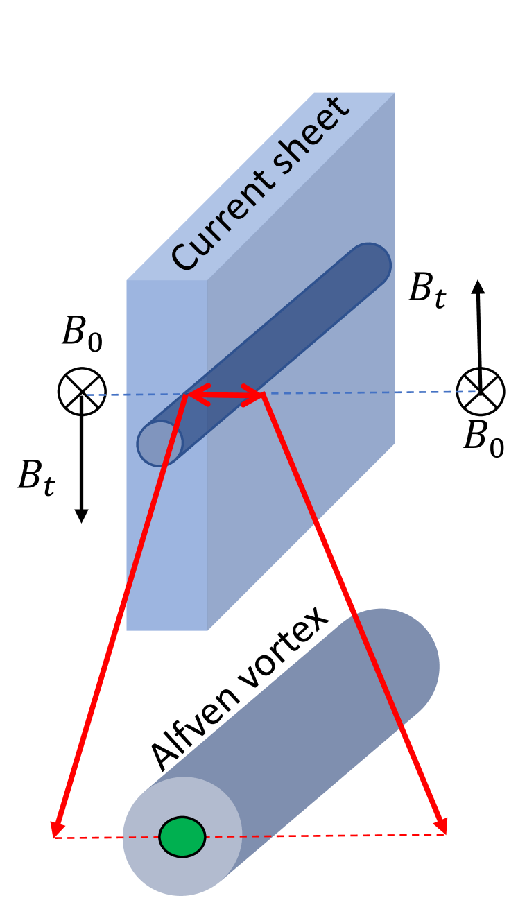
Figure 10: Schematic sketch of the Example 2, shown in the Figure 9. The blue dashed line illustrates the crossing trajectory. The magnetic field fluctuations associated with a vortex are shown in black. The red lines indicate the zoom to the embedded ion-scale vortex. A compressible sub-ion scale vortex is shown in green. The embedded sub-structures are shown not to scale.

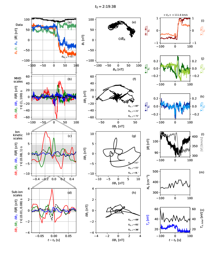
Figure 11: Example 3: A rotational discontinuity (switchback boundary) nested in a larger magnetic depression region on MHD scales. The format is the same as Figure 7.

Figure 7(i-k) show the magnetic field fluctuations normalised by the background magnetic field $(\mathbf{B}-\langle\mathbf{B}\rangle)/B_{0}$, where $B_{0}=\langle|B|\rangle_{t-t_{0}\in(-100,100)s}=100$ nT, and the proton velocity fluctuations $(\mathbf{V}-\langle\mathbf{V}\rangle)/V_{A}$ normalised by the average Alfvén velocity $V_{A}=B_{0}/\sqrt{\mu_{0}N_{e}m_{p}}=104$ km/s. Both $(\mathbf{B}-\langle\mathbf{B}\rangle)/B_{0}$ and $(\mathbf{V}-\langle\mathbf{V}\rangle)/V_{A}$ are shown in magnetic field MVA reference frame calculated using $(\mathbf{B}-\langle\mathbf{B}\rangle)$ vector over the 200 seconds shown. Magnetic field and velocity variations across the sheet ($\Delta$) are nearly aligned $\alpha(\Delta\mathbf{B},\Delta\mathbf{V})=21^{\circ}$. Variations in $(\mathbf{B}-\langle\mathbf{B}\rangle)/B_{0}$ and $(\mathbf{V}-\langle\mathbf{V}\rangle)/V_{A}$ correlate, but the amplitudes are different $(|\Delta\mathbf{V}|/V_{A})_{1}=0.4\cdot(|\Delta\mathbf{B}|/B_{0})_{1}$.

Thus, the discontinuity does not fulfill the Walen relation $\Delta\mathbf{V}=\pm\Delta\mathbf{B}/\sqrt{4\pi\rho}$ for rotational discontinuities. In presence of pressure anisotropy, the density can change across the discontinuity, and the Walen relation is modified, as follows (Hudson, 1970; Neugebauer, 2006):

$$\Delta(A\rho) = 0$$

$$\Delta\mathbf{V} = (\rho/\mu_{0})^{1/2}A^{1/2}\Delta(\mathbf{B}/\rho)$$ (18)

where $A=1-\mu_{0}(p_{\parallel}-p_{\perp})/B^{2}$ is the anisotropy parameter. In the considered time interval $\beta_{p}<0.5$, so $A=1-4\pi(p_{\parallel}-p_{\perp})/B^{2}>1-\beta\sim 0.5$ implies $A^{1/2}>0.7$. However, we would need $A^{1/2}\sim 0.4$ to explain the observated relationship between $\Delta\mathbf{V}$ and $\Delta(\mathbf{B}/\rho)$ with anisotropy.

In Figure 7(l-n) we see how magnetic field modulus $|B|$, velocity modulus $|V|$, electron density $N_{e}$, ion $T_{i}$ and electron $T_{e}$ temperatures change across the structure. Velocity and temperatures stay nearly constant. At the same time, $|B|$ and $N_{e}$ are anti-correlated: while magnetic filed increases by $\Delta|B|=10$ nT, density decreases by $\Delta N_{e}\sim 50$ cm^-3. This is usually observed for convected structures in pressure balance. The observed properties are typical for a tangential discontinuity, where magnetic field and density are not constant across the discontinuity.

Another property to distinguish between RD and TD is the magnitude of the normal magnetic field component $B_{n}$. The divergence-free condition implies that $B_{n}$ must be constant in case of planar geometry. So, MVA minimum variance direction should represent normal to the magnetic sheet, and $B_{3}=B_{n}=$ constant. Next, tangential discontinuities have $B_{n}=0$, but in observations $B_{3}\simeq 70$ nT. These results are obtained in the known limits of MVA since the MVA estimation of the normal to the sheet can differ from normal estimated from multi-spacecraft methods (Horbury et al., 2001; Knetter et al., 2004).

So, to summarize, starting from the largest observed scales and up to the end of the inertial range, we observe a current sheet that can be interpreted in terms of a tangential discontinuity (TD). At ion and sub-ion scale substructures are embedded in this discontinuity. Ion scale structure resembles the dipole Alfvén vortex model (see Section 5 and Figure 7 column (b)). Sub-ion scale structure might represent a compressible vortex (Jovanović et al., 2015). A sketch describing this event is given in Figure 8.

6.2 Example 2

The second example is shown in Figure 9 in the same format as the first event in Figure 7. The central time of the event is 01:19:20 UT. In panel (a) the raw magnetic field is shown in RTN reference frame.

Panel (e) shows the polarization $B_{T}(B_{N})$; out-of-plane $B_{R}$ does not change sign (this structure is not a switchback). The magnetic field deflects twice within the timescale of $\sim 80$ s. Magnetic field on the left side of $t_{0}$ is different from the right hand side: it rotates by $\Delta\zeta=15^{\circ}$ (see Equation (15)). This can be due to a weak ($|\Delta\mathbf{B}|/B_{0}=(\mathbf{B}_{t=-100s}-\mathbf{B}_{t=100s})/B_{0}\simeq 0.3$) rotational current sheet, since the ratio of velocity and magnetic field jumps satisfy the Walen relation |$\Delta\mathbf{V}|/V_{A}=1.03\cdot|\Delta\mathbf{B}|/B_{0}$.

Magnetic fluctuations at the MHD scales $\delta B_{MHD}$ are shown in Figure 9 (b) in the MVA reference frame. The direction of the maximum eigenvector $\mathbf{e}_{1}$ is well-distinguished from intermediate ($\mathbf{e}_{2}$) and minimum ($\mathbf{e}_{3}$) directions since $\lambda_{2}/\lambda_{1}=0.06$, and it is perpendicular to the background magnetic field $\theta_{B_{0},1}=88^{\circ}$. Magnetic and velocity components are well correlated, indicating the Alfvénicity of fluctuations ($\delta\mathbf{B}/B_{0}=\delta\mathbf{V}/V_{A}$), see panels (i-k). The linear polarisation and the shape of the fluctuation profiles ($\delta B_{1}$) are consistent with the crossing of a monopole Alfvén vortex through the center (Section 5.1.1, Figure 7(a)).

The amplitude of the vortex $\delta B_{1}=60$ nT (i.e., from peak to peak $\Delta B/B_{0}\sim 1.2$) well exceeds the level of incoherent signal $2\sigma_{MHD}=22$ nT. Assuming Taylor hypothesis, the diameter of the vortex can be estimated as $d=V\Delta t\sim 3\cdot 10^{4}$ km. PSP trajectory crosses the structure in a plane nearly perpendicular to $B_{0}$ ($\theta_{B_{0},V}=71^{\circ}$).

The variation of the magnetic field modulus is negligible $\delta|B|/B_{0}=0.03$ as well as the variations of $N_{e}$, $T_{e}$ and $T_{p}$, see panels (l-n). The change of $|V|$ (grey line in panel (l)) is due to the superposition of the velocity fluctuation of the Alfvén vortex on the bulk solar speed.

Figure 9(c) shows the ion scale magnetic fluctuations $\delta B_{ion}$ located in the center of the MHD scale Alfvén vortex. The maximum amplitude of the fluctuation: $\max(|\delta B_{1}|)=24$ nT, as well as two secondary peaks on the left and right sides exceed the incoherent threshold $\pm 2\sigma_{ion-scale}$ shown in grey. The polarization is elliptical (panel (g)), and the maximum variance is perpendicular to the local field direction. These observed properties are in agreement with an ion-scale Alfvén vortex crossing with a finite impact distance from its centrum.

Figure 9(d) shows the sub-ion fluctuations $\delta B_{sub-ion}$, which are 10 times more intense than the incoherent threshold. They are quasi-transverse, $\theta_{B_{0},1}=88^{\circ}$ and $\theta_{B_{0},2}=64^{\circ}$, and weekly compressible, $\max(\delta B_{\parallel})\approx\max(\delta B_{3})<0.2\max(\delta B_{1})$. The polarizaion is elliptical. The maximum variance is perpendicular to the local field, as in the case of ion and MHD scale structures. The fluctuations at sub-ion scales can be explained by the electron Alfvén vortex Jovanović et al. (2015).

In summary, in the example of Figure 9, in raw data we observe a weak current sheet with the thickness of the high amplitude MHD scale structure. This current sheet is Alfvénic in nature that is the property of a rotational discontinuity. The MHD structure we can interpret as a monopole Alfvén vortex crossed close to its centrum. Within this monopole Alfvén vortex, we observe smaller scale vortices at ion and sub-ion scales. The sketch of the Example 2 is presented in the Figure 10.

6.3 Example 3

Figure 11 gives a third event observed at 2:19:38 UT. In panel (a) the center of the current sheet is observed at $t-t_{0}=20$ s, when the magnetic field rotates by the angle $\Delta\zeta=110^{\circ}$. $B_{R}$ changes sign across the sheet, so the sheet forms the boundary of a switchback, similarly to observations in (Krasnoselskikh et al., 2020).

In Figure 11(b), MHD scale fluctuations in MVA reference frame are shown. The amplitude of fluctuations, associated with the discontinuity, exceed the level of the incoherent signal (see grey horizontal band). Panels (e-f) show the corresponding polarizations.

The fluctuations are Alfvénic in the vicinity of the discontinuity: $\delta\mathbf{B}/B_{0}\approx\delta\mathbf{V}_{1}/V_{A}$ when $t-t_{0}\in(0,40)$ s, see Figure 11(i-k). But further away from the discontinuity $\Delta B/B_{0}$ and $\Delta V/V_{A}$ have different amplitudes: $\Delta B_{1}/B_{0}\approx 0.5\cdot\Delta V_{1}/V_{A}$.

The magnetic field modulus decreases from 105 nT at the boundaries to 90 nT in the center (panel (l)). The duration of this magnetic cavity is $\Delta t=100$ s, which corresponds to the scale of $\Delta l=\Delta t\cdot V=3.5\cdot 10^{4}$ km. The density $N_{e}$ weakly increases across the discontinuity (Figure 11(m)). The proton temperature $T_{p}$ is higher on the left side of the discontinuity than on the right (Figure 11(n)). It decreases right in the discontinuity center in contrast with a nearly uniform $T_{e}$.

In summary, the current sheet follows the characteristic features of rotational discontinuities (Section 5.2.1), as follows. Within the short time interval near the center of the sheet $t-t_{0}\in(0,40)$ s, the Walen relation is satisfied (panel (i)), and the magnetic field modulus is constant. The polarization of magnetic fluctuations is arch-like, that is typical for rotational discontinuities (Tsurutani et al., 1996; Sonnerup et al., 2010; Haaland et al., 2012; Paschmann et al., 2013).

Magnetic fluctuations at ion scales (Figure 11(c)) are twice above the incoherent threshold. The maximum and intermediate magnetic fluctuations ($\delta B_{1}$ and $\delta B_{2}$) are transverse and have nearly the same amplitude, the polarisation is close to elliptic (Figure 11(g)). The eigenvalue ratios of the structure are $(\lambda_{3}/\lambda_{2},\lambda_{2}/\lambda_{1})=(0.06,0.71)$ (see the "+" marker in Figure 12 in ion-scales panel). The minimum MVA eigenvector $\textbf{e}_{3}$ is well-defined and parallel to the background magnetic field. The described properties (i.e. localised transverse fluctuations with nearly elliptic polarisation) are consistent with the off-center monopole Alfven vortex crossing (Figure 6(a)). The $\textbf{e}_{3}$ gives the direction of the vortex axis, which is parallel to $B_{0}$ according to the model (Section 5.1.1).

The sub-ion scale structure is localised and its amplitude is much higher than the corresponding incoherent threshold (Figure 11(d)). The sub-ion scale structure has typical properties of structures at these scales: $\delta B_{1}$ is Mexican hat-like, significant compressibility $\delta|B|\sim 0.5\,\delta B_{1}$. Such localized compressible magnetic fluctuations at sub-ion scales can be interpreted as the electron Alfvén vortex Jovanović et al. (2015).

6.4 Summary of detected structures

We collected large statistics of coherent structures (Figure 4). At MHD scales some of these events represent isolated current sheets such as tangential and rotational current sheets with two examples shown in Section 6.1 and 6.3 respectively. However, we found that current sheets are not the dominant type of coherent structures. The example in Section 6.2 (Figure 9) is interpreted as the crossing of a monopole vortex along its center (embedded in a weak and large scale rotationnal discontinuity). What is really interesting is that the embedded structures at ion and sub-ion scales are mostly Alfvén vortices, independently on the existence of a current sheet at large scales. In case of CS at large scales, the sub-ion vortices are compressible and in the case of the large scale Alfvén vortex, the small scale vortex is incompressible. The generality of this conclusion will be studied in a future work.

7 Multiscale minimum variance analysis

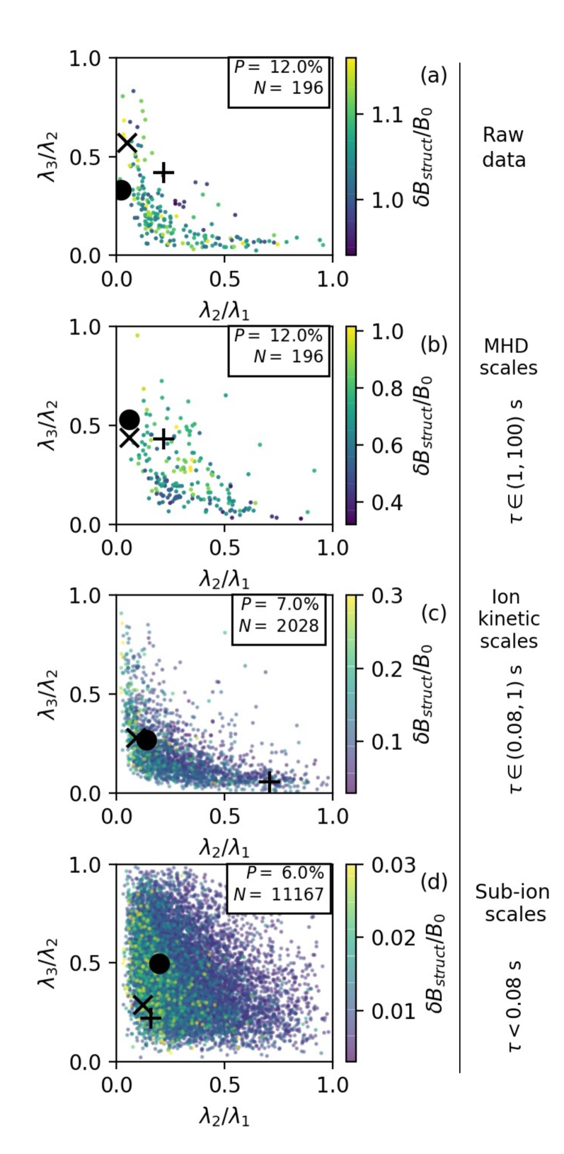
Figure 12: Minimum variance analysis eigenvalues ratios plane ($\lambda_{2}/\lambda_{1},\lambda_{3}/\lambda_{2}$): each dot corresponds to an observed coherent structure, the color gives its amplitude $\delta B_{struct}/B_{0}$. Panels (a,b) correspond to the raw data and MHD scales, respectively. They include 196 structures found at MHD scales. Panel (c) gives results for 2028 structures at ion scales and panel (d) gives the eigenvalues ratios for 11167 events at sub-ion scales. The filling factor $P$ and the number of detected coherent structures $N$ at different frequency ranges are shown in the legends. The eigenvalue ratios of the example structures from Figures 7, 9 and 11 are shown by the black marks: "circle", "cross", and "plus". They correspond to the example structures 1-3, respectively.

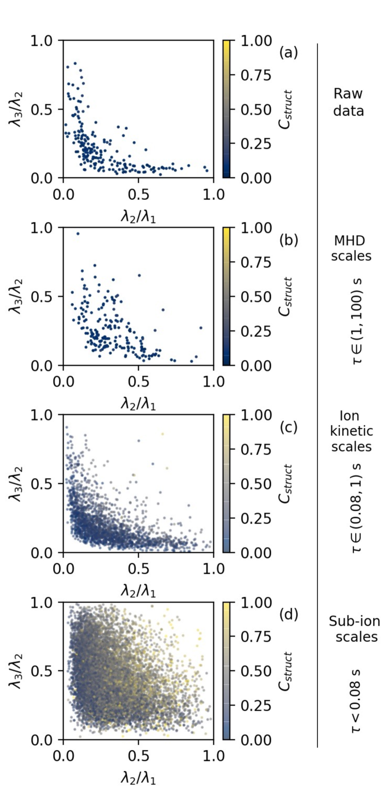
Figure 13: Minimum variance analysis eigenvalues ratios plane ($\lambda_{2}/\lambda_{1},\lambda_{3}/\lambda_{2}$) are shown in the same format as in Figure 12 for the observed coherent structures. The color indicates the compressibility of the coherent structures $C_{struct}$ (defined in Equation (20).

Now, we consider the whole set of structures detected by integrated LIM at different time-scale ranges, see equation (10). As we have discussed in Section 4.1, the number of structures increases toward small scales, from nearly 200 events at MHD scales, to more than $10^{4}$ events at sub-ion scales. For all these events, we study the amplitude anisotropy of the measured fluctuations via minimum variance analysis (MVA). Then, we compare the observed anisotropy with the one of the model structures crossed by a spacecraft. Such synthetic crossings of different models have been already discussed in Section 5 and shown in Figure 6.

7.1 Observational characteristics of coherent structures

For each coherent structure detected at j-th range of scales we consider filtered magnetic field fluctuations $\delta\mathbf{B}_{j}$ at the time interval $t-t_{0}\in T_{struct}=(-\tau_{max,j},\tau_{max,j})$ in the vicinity of the structure center $t_{0}$, where $\tau_{max,j}$ is the maximum timescale of each scale range defined by Equation (7). We define the amplitude of the structure $\delta B_{struct,j}$ as:

$$\delta B_{struct}=\max(|\delta\mathbf{B}_{j}|)_{t\in T_{struct}}$$ (19)

The amplitude anisotropy of the magnetic fluctuations $\delta\mathbf{B}_{j}$ of the structure along the crossing trajectory is characterised by MVA eigenvalue ratios $\lambda_{2}/\lambda_{1}$ and $\lambda_{3}/\lambda_{2}$. The relative amplitude $\delta B_{struct,j}/B_{0}$ is shown in color in the Figure 12. For each range of scales, the number of structures $N$ and the filling factor $P$ are shown in the legend.

Figure 12(a) gives the results of the MVA for the raw magnetic field data during 200 s time intervals around the central times $t_{0}$ of the MHD-scale coherent structures (see the discussion of the detection method in the end of Section 4.1). The MVA results for three examples analysed in detail in Sections 6.1,6.2, and 6.3 are marked on the $(\lambda_{2}/\lambda_{1}$,$\lambda_{3}/\lambda_{2})$ plane with special symbols: Example-1, TD at large scales, is a black dot; Example-2, an Alfvén vortex at large scales, is a cross; and Example-3, a RD at large scales, is a plus. We see here, that intermediate over maximum variance, $\lambda_{2}/\lambda_{1}$, can be anything, as is the case for the monopole and dipole Alfvén vortex, see Figure 6. Minimum over intermediate variance, $\lambda_{3}/\lambda_{2}$, sometime takes high values ($>0.5$), as is the case for the monopole vortex, a tangential discontinuity or a magnetic hole. Values of $\lambda_{3}/\lambda_{2}$ around 0.3 and for small $\lambda_{2}/\lambda_{1}$ can be interpreted as rotational discontinuities, see Figure 6. So, the observed distribution of $\lambda_{3}/\lambda_{2}$ as a function of $\lambda_{2}/\lambda_{1}$ can be due to a superposition of different types of coherent structures. It seems that vortices are dominant, but other types of structures may also exist.

Figure 12(b) corresponds to the same set of coherent structures as in panel (a) but for filtered MHD-scale fluctuations $\delta\mathbf{B}_{MHD}$ instead of the raw magnetic field data. Here, the data are spread nearly uniformly in the bottom-left part of the panel. This distribution can be also interpreted as a superposition of the 5 models discussed above, with a dominance of vortices.

Figure 12(c,d) represent the MVA results for ion and sub-ion scale structures respectively. At ion scales, the distribution is similar to what is observed in raw data, but with more cases (2028 vs 196). Sub-ion scale structures have different distribution on the MVA eigenvalue ratios. Most of the points and especially of high amplitude events are grouped closer the left side of the eigenvalue ratios plane, where $\lambda_{2}/\lambda_{1}<0.25$. But this does not exclude any of the 5 models.

An additional distinguishing parameter is the compressibility of magnetic fluctuations within a coherent structure. A coherent structure is compressible, if the magnetic field magnitude $|B|$ is not constant due to the parallel magnetic fluctuations of the structure. Considering the compressibility at j-th range of scales, we filter $|B|$ (as we do for fluctuations $\delta\mathbf{B}_{j}$) to define $\delta|B|$ at the scale-range $j$. The amplitude of compression associated with a coherent structure is given as $\max(|\delta|B||)_{t\in T_{struct}}$. We normalise it by $\delta B_{struct}$ to define the compressibility of the structure:

$$C_{struct}=\max(|\delta|B||)/\delta B_{struct}$$ (20)

We underline that our definition of compressibility differs from the definitions used in Turner et al. (1977); Volwerk et al. (2020). It is more similar to those used in Stevens & Kasper (2007); Perrone et al. (2016).

Figure 13 shows the MVA eigenvalue ratios of the structures in the same format as the Figure 12, but the color indicates the compressibility $C_{struct}$ (defined in Equation (20)). One observes that in the raw data, at MHD and ion scales, the structures are mostly incompressible, see Figure 13(a-c). At sub-ion scales, incompressible structures are located close to the x-axis as it is expected for vortices and close to y-axis as is expected for current sheets and vortices. The most compressible events (with $C_{struc}\geq 0.8$) represents only $2.7\%$ and can appear anywhere in the plane. At these small scales, $34\%$ of events can not be compared with the 5 models described above. Indeed, these events are the ones from the middle of the plane, around $\lambda_{2}/\lambda_{1}=\lambda_{3}/\lambda_{2}=0.5$, and which have low amplitudes as one can see from Figure 12(d). So, we conclude that at sub-ion scales, low amplitude events have more isotropic magnetic fluctuations.

Below, in Sections 7.2 and 7.3 we use another approach to quantify the proportions of different types of structures at different scales.

7.2 Noise level estimation

We want to compare the observed distributions of $(\lambda_{2}/\lambda_{1},\lambda_{3}/\lambda_{2})$ and the degree of compressibility $C_{struct}$ for MHD, ion and sub-ion scale structures, with the crossings of different coherent structures models, (see Section 5). The incoherent noise affects the MVA eigenvalue ratios (shown in the bottom row of the Figure 6). The greater is the ratio $\epsilon=\delta B_{noise}/\delta B_{struct}$, the closer are the $\lambda_{2}/\lambda_{1}$ and $\lambda_{3}/\lambda_{2})$ to 1. Therefore, we need to estimate $\epsilon$ from observations to take into account the noise in the model crossings.

For each structure at j-th scale range we calculate the ratio of the noise $\sigma_{noise,j}$ (defined in Equation (11)) to the amplitude of the structure $\delta B_{struct,j}$:

$$\epsilon_{obs,j}=\sigma_{noise,j}/\delta B_{struct,j}$$ (21)

At each range of scales the distribution of $\epsilon_{obs,j}$ is nearly Gaussian, but with different values of parameters. The mean values $\langle\epsilon_{obs,j}\rangle$ and the standard deviations $\sigma(\epsilon_{obs,j})$ are shown in the Table 2.

We repeated the crossings simulation with 10 different relative amplitudes of the imposed noise $\epsilon_{sim}$ following the Gaussian distribution with the same parameters, $\langle\epsilon_{obs,j}\rangle$ and $\sigma(\epsilon_{obs,j})$, as in observations. The obtained results of the model crossings with different $\epsilon_{sim}$ are used in the next Section.

	$\langle\epsilon_{obs}\rangle$	$\sigma(\epsilon_{obs,j})$
RAWDATA MHD	0.11	0.03
MHD	0.11	0.03
Ion scales	0.15	0.05
Sub-ion	0.12	0.03

Table 2: The mean and the standard deviation of the relative noise level $\epsilon_{obs}$ at different ranges of scales (defined in Equation (21)).

			Alfvén vortex		Current sheet		Magnetic hole	None
	$N$	$P$ [%]	Monopole	Dipole	Rotational	Tangential
RAWDATA MHD	196	12	0.04	0.86	0.1	0	0	0
MHD	196	12	0.1	0.84	0.0	0	0	0.06
Ion scales	2028	7	0.15	0.85	0.0	0	0	0
Sub-ion	11167	6	0.07	0.49	0.05	0	0.004	0.34

Table 3: In the 1st and 2nd columns, we give the number of structures $N$ and the filling factor $P$ [%] at different ranges of scales (as defined in Section (4.1)). Other columns give results of the problem formulated in Equation (24): the coefficients $p(\text{model})$ which correspond to the fraction of the observed coherent structures that have MVA eigenvalue ratios and compressibility consistent with the crossing of a given model (Figure 6).

7.3 Classification

For convenience we use the notation $(r_{32},r_{21})=(\lambda_{3}/\lambda_{2},\lambda_{2}/\lambda_{1})$ for MVA eigenvalue ratios. First, we systematically investigate the compressible coherent structures with nearly linear polarisation, such as magnetic holes (see Section 5.3). We use two criteria to select magnetic holes. First, $C_{struct}>0.8$ ($C_{struct}$ is defined in Eq. (20)) to select strongly compressible structures and second, we delimit the zone $(r_{32}>0.6,r_{21}<0.4)$ in the MVA eigenvalue ratios plane, that is characteristic for the magnetic hole crossings, see the bottom panel of the Figure 6(e). Their percentage at MHD, ion and subion scales is shown in the column Magnetic hole of Table 3. We found that they are observed only at sub-ion scales. Among sub-ion scale structures, they account for 0.4% of the cases. We will study these events in more details in a future work.

We define the proportions of vortices and current sheets among the remaining observed structures by comparing the amplitude anisotropy from observation, without imposing any criterion for compressibility.

Figure 14(a) show 2D histograms ($6\times 6$ bins) of distributions of the data in $(r_{32},r_{21})$–plane for observations at MHD (top), ion (middle) and sub-ion (bottom) scales. In other words, we show the probability density $P_{obs,j}$ of observations

$$P_{obs,j}(r_{32},r_{21})=N_{obs,j}(r_{32},r_{21})/N_{obs,j},$$ (22)

where $N_{obs,j}(r_{32},r_{21})$ is the number of the observed structures in a bin, and $N_{obs,j}$ is the total number of observed structures. The index $j$ denotes the scale range.

We assume that crossings of coherent structures along trajectories with different impact parameters are equally probable and we take into account the noise from the observations, with Equation (21), as explained below. Since the dipole Alfvén vortex has an angular structure, we average the results over a uniform distribution of trajectory orientations. Then, we obtain the probability density $P(r_{32},r_{21}|\text{model})$ of MVA eigenvalue ratios for each model structure:

$$P_{j}(r_{32},r_{21}|\text{model})=N_{model,j}(r_{32},r_{21})/N_{model,j}$$ (23)

The probability distributions for 4 different models $P_{j}(r_{32},r_{21}|\text{model})$ are shown in columns (b-e) of Figure 14. To simulate different scales, we change the level of the noise according to what is observed at each scale, see Equation (21).

The observed distribution of MVA eigenvalue ratios $P_{obs,j}$ can be expressed as the linear combination of the conditional probabilities $P_{j}(r_{32},r_{21}|\text{model})$, determined from the models. The positive coefficients $p(\text{model})$ reflect the probability to encounter each model structure. Coefficients $p(\text{model})$ are found from the constrained minimisation problem:

$$\begin{cases}||P_{obs}(r_{32},r_{21})-\displaystyle\sum_{model}p(\text{model})P(r_{32},r_{21}|\text{model})||\to 0\\ \displaystyle\sum_{model}p(\text{model})\leq 1\\ p(\text{model})\geq 0\end{cases}$$ (24)

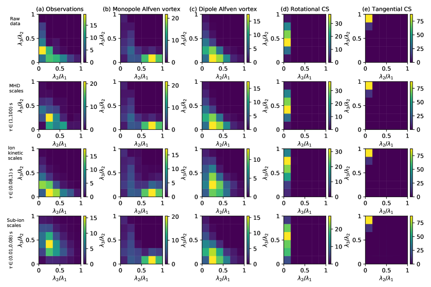
Figure 14: Probability distributions on the MVA eigenvalue ratios plane $(r_{32},r_{21})=(\lambda_{3}/\lambda_{2},\lambda_{2}/\lambda_{1})$. The column (a) shows the probability [%] per bin to observe a coherent structure with the corresponding MVA eigenvalue ratios (so $P_{obs,j}(r_{32},r_{21})$ defined by Equation (22)). First and second panels of the column (a) show the distributions for the MHD-scale coherent structures using the raw (non-filtered) data and the MHD-range filtered data respectively. Third and fourth rows of the column (a) correspond to coherent structures detected at ion and sub-ion scale ranges respectively. Columns (b-e) show the probability densities obtained from simulating model crossings ($P_{j}(r_{32},r_{21}|\text{model})$ defined by Equation (23)). The difference between panels in columns (b-e) is due to the different imposed noise level $\epsilon_{sim}$ (see Section 7.2 for details).

We use the least squares minimisation. The resulting probabilities $p(\text{model})$ at different scales and for different models are shown in the Table 3: The MVA eigenvalues of the observed coherent structures at any scale range are most consistent with the crossings of the dipole Alfvén vortices. The monopole vortices account for $7-15\%$ of coherent structures among different scales. The rotational discontinuities are observed in raw (non-filtered) data at MHD scales only. Tangential discontinuities does not appear to be statistically significant. There is $6\%$ of events which were not possible to model at MHD scales and nearly $40\%$ at sub-ion scales (see the None column in Table 2). These unidentified large number of events at sub-ion scales is probably due to a more 3-dimentional nature of the fluctuations not taken into account by nearly incompressible models.

The result presented in Table 3 doesn’t change qualitatively if instead of least squares, the sum of the absolute values of probability differences (between observations and models) in each bin is minimized.

8 Conclusion and discussions

The intermittency in the solar wind is typically investigated from the statistical point of view. The scale-dependent kurtosis of magnetic increments is used as the principal quantitative diagnostic, showing the presence of coherent structures.

In this paper, for the first time, we apply a multi-scale approach in physical space, from the largest MHD scales, to the smallest resolved sub-ion scales.

Using PSP merged magnetic field data at 0.17 au and the Morlet wavelet transform, we detect intermittent coherent structures (appearing as vertical elongations from MHD to sub-ion scales in magnetic scalogram) and we apply the multi-scale analysis for each detected event. Around each central time of an event, we find localised magnetic fluctuations at sub-ion scales with amplitudes up to $\delta B/B_{0}\sim 0.03$. This small scale event is embedded in a larger event at ion scales, with amplitudes up to $\delta B/B_{0}\sim 0.3$. At its turn, ion scale event is embedded in a high-amplitude ($\delta B_{struct}/B_{0}\sim 0.4-1.0$) MHD-scale structures. Such embedding across the whole turbulent cascade is presented here for the first time.

The topology and properties of the coherent structures change from scale to scale. Using plasma and field time profiles, we could characterize several events in more details. We show examples of planar tangential and rotational discontinuities at MHD scales containing embedded cylindrical sub-structures inside it: incompressible ion-scale Alfvén vortex and sub-ion scale compressible vortex. Another example is a cylindrical structure of vortex type at MHD, with embedded incompressible vortices at ion and sub-ion scales.

From the analysed examples, we see that while at large scales a planar discontinuity is present, the sub-ion scale vortex is compressible. However, if the large scale MHD vortex is present, like in Example-2, the sub-ion scales vortex can be nearly incompressible.

We completed study of examples with a statistical analysis. In a time interval of about 5 hours we detected nearly 200 events at the MHD scales, and much more events at ion ($\sim 2\cdot 10^{3}$) and sub-ion scales ($\sim 10^{4}$).

The filling factor of the structures, that we estimate in a conservative way (see discussion in section 4.1), decreases from 12% at MHD scales to 7% and 6% at ion and sub-ion scales correspondingly. However, the tails of the PDF’s of magnetic fluctuations within different scale ranges, increases toward smaller scales.

In order to determine the dominant type of coherent structures, we compare observations with models of Alfvén vortices (monopole and dipole), current sheets (tangential and rotational discontinuities), and magnetic holes. The amplitude anisotropy of magnetic fluctuations, measured along the crossing trajectory, is quantified with the two ratios of minimum variance (MVA) eigenvalues. The model crossings are simulated along a set of trajectories with a broad range of impact parameter. The statistics of crossings shows that each model structure has a distinctive most-probable zone in the eigenvalue ratios plane. We fit the distribution of eigenvalue ratios from observations with the linear combination of the distributions obtained with the model crossings. This provides the proportions of the vortices and current sheets.

At the MHD scales applying MVA to the raw data we found 86% dipole Alfvén vortices, 4% monopole vortices and 10% rotational discontinuities. Analyzing the same structures with filtered magnetic field data at MHD scales, $(1,100)$ s, we found 84% dipole vortices, 10% monopole vortices, and 6% unspecified structures. The discontinuities found in raw data are rarely isolated (an isolated current sheet is Example 1, Figure 7). Thus, while considering only time scales below 100 s, the amplitude of the jump decreases and the MVA results give properties of MHD structures around the discontinuity, as is clearly seen in Example 3, Figure 11.

On ion scales we found 85% dipole vortices and 15% of monopoles. Planar discontinuities are not found by our method.

On subion scales coherent structures represent dipole vortices (49%), monopole vortices (7%), rotational current sheets (5%) and magnetic holes (0.4%). Around 34% of sub-ion scale structures don’t fit any of the considered models. It is plausibly, because the incompressible models of vortices have been used in comparison to observations. To improve this study at sub-ion scales in the future, the electron-scale Alfvén vortex model of Jovanović et al. (2015) should be used.

The visual classification of ion-scale coherent structures at 0.17 au, during the first PSP perihelion, has been done recently in Perrone et al. (2020). Three different time intervals were considered: quiet, weekly-disturbed and highly-disturbed solar wind. The highly-disturbed interval (of 1.5 h) with $B_{R}$ reversals is a subset of the 5h-interval considered here. The authors concluded that in the highly-disturbed interval current sheets were dominant ($46$%), while during the weekly-disturbed interval Alfvén vortices ($45$%) and wave packets ($50$%) were observed. This is in contrast with the quantitative classification presented in this article (showing that Alfvén vortices are dominant).

In the previous studies of ion scales coherent structures at 1 au in slow (Perrone et al., 2016) and fast (Perrone et al., 2017) solar wind with Cluster satellites, the dominance of Alfvén vortices with respect to current sheets has been found. That is more consistent with our results at 0.17 au in the slow wind.

Results presented in this article are limited to a specific slow highly-perturbed solar wind region at 0.17 au from the Sun. The analysis can be expanded to different solar wind conditions (different radial distance, types of solar wind, originating from ecliptic or polar regions of the Sun) in order to obtain a more general picture. An interesting problem is how the structures evolve in the same plasma parcel as the solar wind expands.

To identify exactly the same plasma at different radial distances is not an evident task. Several studies gives attempt to do so with PSP and SOLO and study the evolution of statistical turbulence properties (for example, Telloni et al., 2021) and intermittency (Sioulas et al., 2022). Perrone et al. (2022) compared the solar wind from the same coronal hole observed by PSP at 0.1 au and by SOLO at 0.97 au. The authors show examples of vortex like structures at ion scales at these two radial distances with 0.7 s duration at 0.1 au and 4 s duration at 0.97 au. This increase of time scale with $R$ is consistent with radial evolution of spatial ion scales such as ion inertial length $\lambda_{i}$ and ion Larmor radius $\rho_{i}$. The evolution of current sheets in similar solar wind was investigated during the ARTEMIS P1 (at 1 au) and MAVEN (at Mars orbit) alignment Artemyev et al. (2018). However, in similar solar wind we can not study coherent structures evolution and stability, only following the same plasma parcel can give such a possibility.

Multiscale nature of coherent strucutres described in this article can be studied in future by the Helioswarm (accepted NASA mission). It will cover MHD, ion and sub-ion scales at the same time.

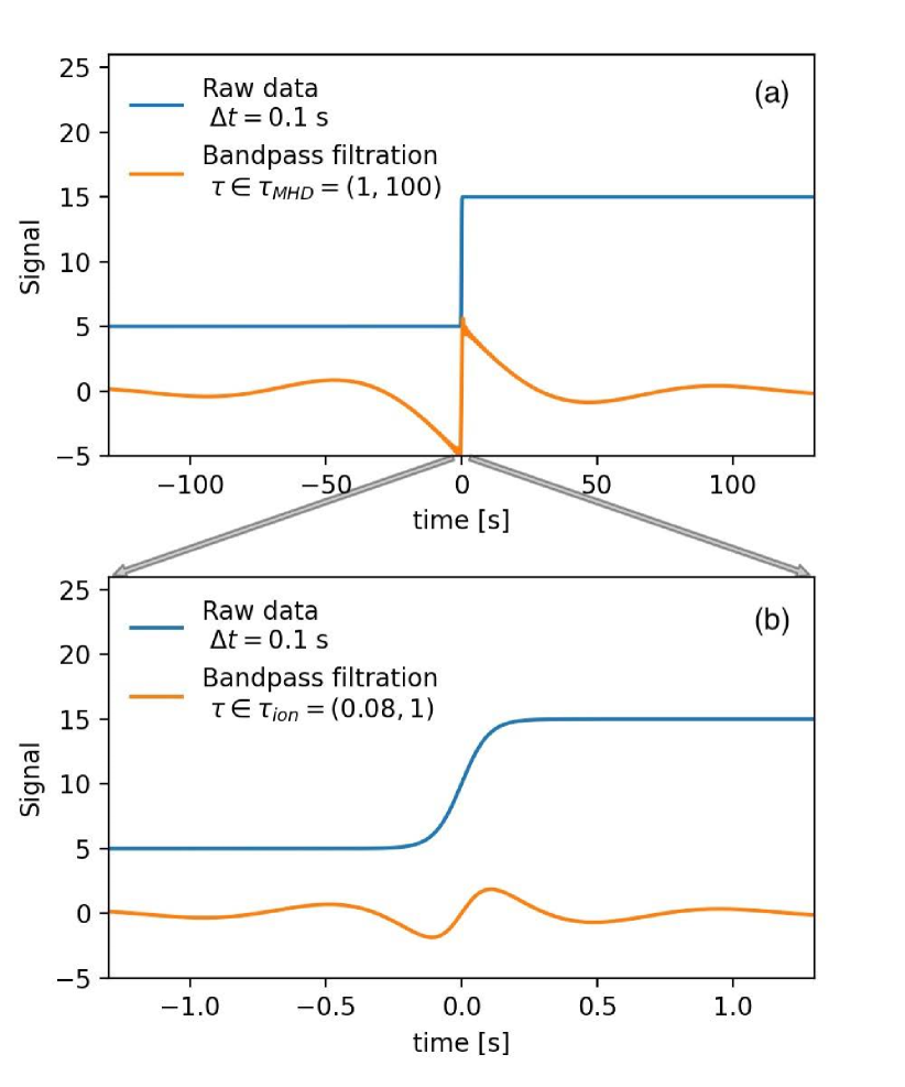
Figure 15: Filtration of the current sheet. The temporal scale of the current sheet is $\Delta t=0.1$ s. The top panel (a) shows the raw data (blue line) and the bandpass filtered signal at MHD range of timescales $\tau\in\tau_{MHD}$ (orange). The bottom panel shows the zoom to the shorter time interval. The same raw data as in panel (a) is shown in blue. The orange line in panel (b) shows the bandpass filtration at $\tau\in\tau_{ion}$.

At ion and sub-ion scales the size and amplitude of embedded substructures are much smaller than the the background and MHD-scale fluctuations. Therefore, filtration allows to remove the quasi-constant background and to analyze specifically the fluctuations associated with substructures. However, the filtration may introduce an ambiguity in the interpretation of the signal. Consider the thin (i.e. $\ell\sim d_{i}$) current sheet, so that the crossing duration is $\Delta t=0.125$ s. Figure 15 shows the tangential magnetic field component of the current sheet (blue) and the result of the filtration (orange).

In Figure 15(a) the filter frequency window corresponds to the MHD inertial range, as defined in Section 3 in Equation 6. Since the thickness of the sheet is small, $\Delta t/\text{min}(\tau_{MHD})=0.1$, the filtered signal has a steep jump of the same amplitude as the amplitude of the initial signal. However, unlike the initial signal, the filtered signal tends to 0 at the scale $|t|>\text{max}(\tau_{MHD})/2$ away from the discontinuity. Two small peaks appear at $t=\pm 50$ s.

Figure 15(b) shows the result of the filtration at ion scales. The magnetic field changes sign smoothly. If the thickness of an intense coherent structure is smaller than the minimum timescale of the MHD range, and if the classification method is based on the shape of the most intense filtered magnetic field component, then the CS filtration remnant at ion scales can be miss-classified as an embedded monopole Alfven vortex crossed through its center.

Alternatively, the classification can be based on the observational statistics of MVA eigenvalue ratios. MVA eigenvalue ratios $(\lambda_{3}/\lambda_{2},\lambda_{2}/\lambda_{1})$ characterise the amplitude anisotropy of the magnetic fluctuations along the crossing trajectory. Moreover, the classification based on the probability distributions of MVA eigenvalue ratios indirectly takes into account the geometry of the structures, because the probability of having different ($\lambda_{3}/\lambda_{2},\lambda_{2}/\lambda_{1}$) depends on the geometry of the structure and on the crossing trajectory. Indeed, in Section 5 it was shown that in case of Alfven vortices (unlike current sheets) crossing $(\lambda_{3}/\lambda_{2},\lambda_{2}/\lambda_{1})$ depend strongly on the impact parameter $\phi$. The observed probability distribution of $(\lambda_{3}/\lambda_{2},\lambda_{2}/\lambda_{1})$ is a global characteristics of coherent structures, if we assume, that in observations there is no preferential impact parameter (all $\phi$ shown in the blue cone in Figure 6 have equal probability).

References

- Alexandrova (2008) Alexandrova, O. 2008, Nonlinear Processes in Geophysics, 15, 95, doi: 10.5194/npg-15-95-2008
- Alexandrova (2020) Alexandrova, O. 2020, Habilitation à diriger des recherches, Observatoire de Paris, Université Paris Sciences et Lettres (PSL). https://hal.science/tel-03999422
- Alexandrova et al. (2013) Alexandrova, O., Chen, C. H. K., Sorriso-Valvo, L., Horbury, T. S., & Bale, S. D. 2013, Space Sci. Rev., 178, 101, doi: 10.1007/s11214-013-0004-8
- Alexandrova et al. (2021) Alexandrova, O., Jagarlamudi, V. K., Hellinger, P., et al. 2021, Phys. Rev. E, 103, 063202, doi: 10.1103/PhysRevE.103.063202
- Alexandrova et al. (2012) Alexandrova, O., Lacombe, C., Mangeney, A., Grappin, R., & Maksimovic, M. 2012, ApJ, 760, 121, doi: 10.1088/0004-637X/760/2/121
- Alexandrova et al. (2006) Alexandrova, O., Mangeney, A., Maksimovic, M., et al. 2006, Journal of Geophysical Research (Space Physics), 111, A12208, doi: 10.1029/2006JA011934
- Alexandrova & Saur (2008) Alexandrova, O., & Saur, J. 2008, Geophys. Res. Lett., 35, L15102, doi: 10.1029/2008GL034411
- Alexandrova et al. (2009) Alexandrova, O., Saur, J., Lacombe, C., et al. 2009, Phys. Rev. Lett., 103, 165003, doi: 10.1103/PhysRevLett.103.165003
- Alterman & Kasper (2019) Alterman, B. L., & Kasper, J. C. 2019, ApJ, 879, L6, doi: 10.3847/2041-8213/ab2391
- Artemyev et al. (2018) Artemyev, A. V., Angelopoulos, V., Halekas, J. S., et al. 2018, ApJ, 859, 95, doi: 10.3847/1538-4357/aabe89
- Artemyev et al. (2019) Artemyev, A. V., Angelopoulos, V., & Vasko, I. Y. 2019, Journal of Geophysical Research (Space Physics), 124, 3858, doi: 10.1029/2019JA026597
- Bale et al. (2016) Bale, S. D., Goetz, K., Harvey, P. R., et al. 2016, Space Sci. Rev., 204, 49, doi: 10.1007/s11214-016-0244-5
- Bale et al. (2019) Bale, S. D., Badman, S. T., Bonnell, J. W., et al. 2019, Nature, 576, 237, doi: 10.1038/s41586-019-1818-7
- Baumjohann & Treumann (1997) Baumjohann, W., & Treumann, R. A. 1997, Basic Space Plasma Physics (Imperial College Press)
- Borovsky (2008) Borovsky, J. E. 2008, Journal of Geophysical Research (Space Physics), 113, A08110, doi: 10.1029/2007JA012684
- Bowen et al. (2020) Bowen, T. A., Bale, S. D., Bonnell, J. W., et al. 2020, Journal of Geophysical Research (Space Physics), 125, e27813, doi: 10.1029/2020JA027813
- Bruno (2019) Bruno, R. 2019, Earth and Space Science, 6, 656, doi: 10.1029/2018EA000535
- Bruno et al. (2001) Bruno, R., Carbone, V., Veltri, P., Pietropaolo, E., & Bavassano, B. 2001, Planet. Space Sci., 49, 1201, doi: 10.1016/S0032-0633(01)00061-7
- Burlaga (1969) Burlaga, L. F. 1969, Sol. Phys., 7, 54, doi: 10.1007/BF00148406
- Chasapis et al. (2015) Chasapis, A., Retinò, A., Sahraoui, F., et al. 2015, ApJ, 804, L1, doi: 10.1088/2041-8205/804/1/L1
- Chen et al. (2010) Chen, C. H. K., Horbury, T. S., Schekochihin, A. A., et al. 2010, Phys. Rev. Lett., 104, 255002, doi: 10.1103/PhysRevLett.104.255002
- Chen et al. (2020) Chen, C. H. K., Bale, S. D., Bonnell, J. W., et al. 2020, ApJS, 246, 53, doi: 10.3847/1538-4365/ab60a3
- Eastwood et al. (2021) Eastwood, J. P., Stawarz, J. E., Phan, T. D., et al. 2021, A&A, 656, A27, doi: 10.1051/0004-6361/202140949
- Farge (1992) Farge, M. 1992, Annual Review of Fluid Mechanics, 24, 395, doi: 10.1146/annurev.fl.24.010192.002143
- Farge & Schneider (2015) Farge, M., & Schneider, K. 2015, Journal of Plasma Physics, 81, doi: 10.1017/s0022377815001075
- Feng et al. (2008) Feng, H. Q., Wu, D. J., Lin, C. C., et al. 2008, Journal of Geophysical Research (Space Physics), 113, A12105, doi: 10.1029/2008JA013103
- Fiedler (1988) Fiedler, H. E. 1988, Progress in Aerospace Sciences, 25, 231, doi: 10.1016/0376-0421(88)90001-2
- Goodrich & Cargill (1991) Goodrich, C. C., & Cargill, P. J. 1991, Geophys. Res. Lett., 18, 65, doi: 10.1029/90GL02436
- Greco et al. (2008) Greco, A., Chuychai, P., Matthaeus, W. H., Servidio, S., & Dmitruk, P. 2008, Geophys. Res. Lett., 35, L19111, doi: 10.1029/2008GL035454
- Greco et al. (2012) Greco, A., Matthaeus, W. H., D’Amicis, R., Servidio, S., & Dmitruk, P. 2012, ApJ, 749, 105, doi: 10.1088/0004-637X/749/2/105
- Greco et al. (2018) Greco, A., Matthaeus, W. H., Perri, S., et al. 2018, Space Sci. Rev., 214, 1, doi: 10.1007/s11214-017-0435-8
- Greco et al. (2009) Greco, A., Matthaeus, W. H., Servidio, S., Chuychai, P., & Dmitruk, P. 2009, ApJ, 691, L111, doi: 10.1088/0004-637X/691/2/L111
- Greco et al. (2016) Greco, A., Perri, S., Servidio, S., Yordanova, E., & Veltri, P. 2016, ApJ, 823, L39, doi: 10.3847/2041-8205/823/2/L39
- Haaland et al. (2012) Haaland, S., Sonnerup, B., & Paschmann, G. 2012, Annales Geophysicae, 30, 867, doi: 10.5194/angeo-30-867-2012
- Hada et al. (2003) Hada, T., Koga, D., & Yamamoto, E. 2003, Space Sci. Rev., 107, 463, doi: 10.1023/A:1025506124402
- Harris (1962) Harris, E. G. 1962, Il Nuovo Cimento, 23, 115, doi: 10.1007/BF02733547
- Haynes et al. (2015) Haynes, C. T., Burgess, D., Camporeale, E., & Sundberg, T. 2015, Physics of Plasmas, 22, 012309, doi: 10.1063/1.4906356
- Horbury et al. (2001) Horbury, T. S., Burgess, D., Fränz, M., & Owen, C. J. 2001, Geophys. Res. Lett., 28, 677, doi: 10.1029/2000GL000121
- Hudson (1970) Hudson, P. D. 1970, Planet. Space Sci., 18, 1611, doi: 10.1016/0032-0633(70)90036-X
- Hussain (1986) Hussain, A. K. M. F. 1986, Journal of Fluid Mechanics, 173, 303, doi: 10.1017/S0022112086001192
- Janvier et al. (2014) Janvier, M., Démoulin, P., & Dasso, S. 2014, Sol. Phys., 289, 2633, doi: 10.1007/s11207-014-0486-x
- Jovanović et al. (2018) Jovanović, D., Alexandrova, O., Maksimović, M., & Belić, M. 2018, Journal of Plasma Physics, 84, 725840402, doi: 10.1017/S002237781800082X
- Jovanović et al. (2015) Jovanović, D., Alexandrova, O., & Maksimović, M. 2015, Physica Scripta, 90, 088002, doi: 10.1088/0031-8949/90/8/088002
- Kadomtsev & Pogutse (1974) Kadomtsev, B. B., & Pogutse, O. P. 1974, Soviet Journal of Experimental and Theoretical Physics, 38, 283
- Karimabadi et al. (2013) Karimabadi, H., Roytershteyn, V., Wan, M., et al. 2013, Physics of Plasmas, 20, 012303, doi: 10.1063/1.4773205
- Kasper et al. (2007) Kasper, J. C., Stevens, M. L., Lazarus, A. J., Steinberg, J. T., & Ogilvie, K. W. 2007, ApJ, 660, 901, doi: 10.1086/510842
- Kasper et al. (2016) Kasper, J. C., Abiad, R., Austin, G., et al. 2016, Space Sci. Rev., 204, 131, doi: 10.1007/s11214-015-0206-3
- Kasper et al. (2019) Kasper, J. C., Bale, S. D., Belcher, J. W., et al. 2019, Nature, 576, 228, doi: 10.1038/s41586-019-1813-z
- Kiyani et al. (2015) Kiyani, K. H., Osman, K. T., & Chapman, S. C. 2015, Philosophical Transactions of the Royal Society of London Series A, 373, 20140155, doi: 10.1098/rsta.2014.0155
- Knetter et al. (2004) Knetter, T., Neubauer, F. M., Horbury, T., & Balogh, A. 2004, Journal of Geophysical Research (Space Physics), 109, A06102, doi: 10.1029/2003JA010099
- Koga & Hada (2003) Koga, D., & Hada, T. 2003, Space Sci. Rev., 107, 495, doi: 10.1023/A:1025510225311
- Krasnoselskikh et al. (2020) Krasnoselskikh, V., Larosa, A., Agapitov, O., et al. 2020, ApJ, 893, 93, doi: 10.3847/1538-4357/ab7f2d
- Kuzzay et al. (2019) Kuzzay, D., Alexandrova, O., & Matteini, L. 2019, Phys. Rev. E, 99, 053202, doi: 10.1103/PhysRevE.99.053202
- Lacombe et al. (2017) Lacombe, C., Alexandrova, O., & Matteini, L. 2017, ApJ, 848, 45, doi: 10.3847/1538-4357/aa8c06
- Li et al. (2011) Li, G., Miao, B., Hu, Q., & Qin, G. 2011, Phys. Rev. Lett., 106, 125001, doi: 10.1103/PhysRevLett.106.125001
- Lion et al. (2016) Lion, S., Alexandrova, O., & Zaslavsky, A. 2016, ApJ, 824, 47, doi: 10.3847/0004-637X/824/1/47
- Lotekar et al. (2022) Lotekar, A. B., Vasko, I. Y., Phan, T., et al. 2022, ApJ, 929, 58, doi: 10.3847/1538-4357/ac5bd9
- Mangeney (2001) Mangeney, A. 2001, in ESA Special Publication, Vol. 492, Sheffield Space Plasma Meeting: Multipoint Measurements versus Theory, ed. B. Warmbein, 53
- Matteini et al. (2020) Matteini, L., Franci, L., Alexandrova, O., et al. 2020, Frontiers in Astronomy and Space Sciences, 7, 83, doi: 10.3389/fspas.2020.563075
- Moldwin et al. (2000) Moldwin, M. B., Ford, S., Lepping, R., Slavin, J., & Szabo, A. 2000, Geophys. Res. Lett., 27, 57, doi: 10.1029/1999GL010724
- Moncuquet et al. (2020) Moncuquet, M., Meyer-Vernet, N., Issautier, K., et al. 2020, ApJS, 246, 44, doi: 10.3847/1538-4365/ab5a84
- Neugebauer (1989) Neugebauer, M. 1989, Geophys. Res. Lett., 16, 1261, doi: 10.1029/GL016i011p01261
- Neugebauer (2006) —. 2006, Journal of Geophysical Research (Space Physics), 111, A04103, doi: 10.1029/2005JA011497
- Osman et al. (2011) Osman, K. T., Matthaeus, W. H., Greco, A., & Servidio, S. 2011, ApJ, 727, L11, doi: 10.1088/2041-8205/727/1/L11
- Papini et al. (2021) Papini, E., Cicone, A., Franci, L., et al. 2021, ApJ, 917, L12, doi: 10.3847/2041-8213/ac11fd
- Paschmann & Daly (1998) Paschmann, G., & Daly, P. W. 1998, ISSI Scientific Reports Series, 1
- Paschmann et al. (2013) Paschmann, G., Haaland, S., Sonnerup, B., & Knetter, T. 2013, Annales Geophysicae, 31, 871, doi: 10.5194/angeo-31-871-2013
- Perrone et al. (2016) Perrone, D., Alexandrova, O., Mangeney, A., et al. 2016, ApJ, 826, 196, doi: 10.3847/0004-637X/826/2/196
- Perrone et al. (2017) Perrone, D., Alexandrova, O., Roberts, O. W., et al. 2017, ApJ, 849, 49, doi: 10.3847/1538-4357/aa9022
- Perrone et al. (2020) Perrone, D., Bruno, R., D’Amicis, R., et al. 2020, ApJ, 905, 142, doi: 10.3847/1538-4357/abc480
- Perrone et al. (2022) Perrone, D., Perri, S., Bruno, R., et al. 2022, A&A, 668, A189, doi: 10.1051/0004-6361/202243989
- Petviashvili & Pokhotelov (1992) Petviashvili, V., & Pokhotelov, O. 1992, Solitary waves in plasmas and in the atmosphere.
- Riley et al. (1996) Riley, P., Sonett, C. P., Tsurutani, B. T., et al. 1996, J. Geophys. Res., 101, 19987, doi: 10.1029/96JA01743
- Roberts et al. (2016) Roberts, O. W., Li, X., Alexandrova, O., & Li, B. 2016, Journal of Geophysical Research (Space Physics), 121, 3870, doi: 10.1002/2015JA022248
- Roytershteyn et al. (2015) Roytershteyn, V., Karimabadi, H., & Roberts, A. 2015, Philosophical Transactions of the Royal Society of London Series A, 373, 20140151, doi: 10.1098/rsta.2014.0151
- Salem (2000) Salem, C. 2000, PhD thesis. http://www.theses.fr/2000PA077264
- Salem et al. (2009) Salem, C., Mangeney, A., Bale, S. D., & Veltri, P. 2009, ApJ, 702, 537, doi: 10.1088/0004-637X/702/1/537
- Salem et al. (2012) Salem, C. S., Howes, G. G., Sundkvist, D., et al. 2012, ApJ, 745, L9, doi: 10.1088/2041-8205/745/1/L9
- Servidio et al. (2008) Servidio, S., Matthaeus, W. H., & Dmitruk, P. 2008, Phys. Rev. Lett., 100, 095005, doi: 10.1103/PhysRevLett.100.095005
- Sioulas et al. (2022) Sioulas, N., Shi, C., Huang, Z., & Velli, M. 2022, ApJ, 935, L29, doi: 10.3847/2041-8213/ac85de
- Siscoe et al. (1968) Siscoe, G. L., Davis, L., J., Coleman, P. J., J., Smith, E. J., & Jones, D. E. 1968, J. Geophys. Res., 73, 61, doi: 10.1029/JA073i001p00061
- Sonnerup et al. (2010) Sonnerup, B. U. Ö., Haaland, S. E., & Paschmann, G. 2010, Annales Geophysicae, 28, 1229, doi: 10.5194/angeo-28-1229-2010
- Sonnerup & Scheible (1998) Sonnerup, B. U. Ö., & Scheible, M. 1998, ISSI Scientific Reports Series, 1, 185
- Stevens & Kasper (2007) Stevens, M. L., & Kasper, J. C. 2007, Journal of Geophysical Research (Space Physics), 112, A05109, doi: 10.1029/2006JA012116
- Strauss (1976) Strauss, H. R. 1976, Physics of Fluids, 19, 134, doi: 10.1063/1.861310
- Telloni et al. (2021) Telloni, D., Sorriso-Valvo, L., Woodham, L. D., et al. 2021, ApJ, 912, L21, doi: 10.3847/2041-8213/abf7d1
- Torrence & Compo (1998) Torrence, C., & Compo, G. P. 1998, Bulletin of the American Meteorological Society, 79, 61, doi: 10.1175/1520-0477(1998)079<0061:APGTWA>2.0.CO;2
- Tsurutani et al. (1996) Tsurutani, B. T., Ho, C. M., Arballo, J. K., et al. 1996, J. Geophys. Res., 101, 11027, doi: 10.1029/95JA03479
- Tsurutani et al. (2011) Tsurutani, B. T., Lakhina, G. S., Verkhoglyadova, O. P., et al. 2011, Journal of Atmospheric and Solar-Terrestrial Physics, 73, 5, doi: 10.1016/j.jastp.2010.04.001
- Turner et al. (1977) Turner, J. M., Burlaga, L. F., Ness, N. F., & Lemaire, J. F. 1977, J. Geophys. Res., 82, 1921, doi: 10.1029/JA082i013p01921
- Veltri (1999) Veltri, P. 1999, Plasma Physics and Controlled Fusion, 41, A787, doi: 10.1088/0741-3335/41/3A/071
- Verkhoglyadova et al. (2003) Verkhoglyadova, O. P., Dasgupta, B., & Tsurutani, B. T. 2003, Nonlinear Processes in Geophysics, 10, 335, doi: 10.5194/npg-10-335-2003
- Volwerk et al. (2020) Volwerk, M., Goetz, C., Plaschke, F., et al. 2020, Annales Geophysicae, 38, 51, doi: 10.5194/angeo-38-51-2020
- Wan et al. (2012) Wan, M., Matthaeus, W. H., Karimabadi, H., et al. 2012, Phys. Rev. Lett., 109, 195001, doi: 10.1103/PhysRevLett.109.195001
- Wang et al. (2020) Wang, G. Q., Zhang, T. L., Xiao, S. D., et al. 2020, Journal of Geophysical Research (Space Physics), 125, e28320, doi: 10.1029/2020JA028320
- Wang et al. (2019) Wang, T., Alexandrova, O., Perrone, D., et al. 2019, ApJ, 871, L22, doi: 10.3847/2041-8213/aafe0d10.48550/arXiv.1901.03869
- Wu et al. (2013) Wu, P., Perri, S., Osman, K., et al. 2013, ApJ, 763, L30, doi: 10.1088/2041-8205/763/2/L30
- Zhao et al. (2020) Zhao, L. L., Zank, G. P., Adhikari, L., et al. 2020, ApJS, 246, 26, doi: 10.3847/1538-4365/ab4ff1
- Zhdankin et al. (2012) Zhdankin, V., Boldyrev, S., Mason, J., & Perez, J. C. 2012, Phys. Rev. Lett., 108, 175004, doi: 10.1103/PhysRevLett.108.175004
- Zhdankin et al. (2013) Zhdankin, V., Uzdensky, D. A., Perez, J. C., & Boldyrev, S. 2013, ApJ, 771, 124, doi: 10.1088/0004-637X/771/2/124