Lasso and elastic nets by orthants

Abstract

We propose a new method for computing the lasso path, using the fact that the Manhattan norm of the coefficient vector is linear over every orthant of the parameter space. We use simple calculus and present an algorithm in which the lasso path is series of orthant moves. Our proposal gives the same results as standard literature, with the advantage of neat interpretation of results and explicit lasso formulæ. We extend this proposal to elastic nets and obtain explicit, exact formulæ for the elastic net path, and with a simple change, our lasso algorithm can be used for elastic nets. We present computational examples and provide simple R prototype code.

Keywords— Lasso, quadratic form, elastic net, regression, regularization.

1 Introduction

This paper is concerned with penalised estimation for the linear regression model

$$\mathbf{Y}=\mathbf{X}\beta+\epsilon.$$ (1)

The vector of response values is $\mathbf{Y}$, the parameter vector is $\beta$; the covariate matrix $\mathbf{X}$ has $p$ linearly independent columns and $n$ rows, one for every observation and $\epsilon$ is the vector of normal independent error terms with zero mean and variance $\sigma^{2}$. In this paper, $\mathbf{Y}$ and $\mathbf{X}$ refer to the observed response vector and covariate matrix, respectively. Following lasso practice, both $\mathbf{Y}$ and columns of $\mathbf{X}$ are centered around their sample means so the regression does not have intercept term.

1.1 Lasso regularization

For parameter estimation of model (1), the Lasso [1] minimizes the criterion

$$L=\frac{1}{2}||\mathbf{Y}-\mathbf{X}\beta||_{2}^{2}+\lambda||\beta||_{1},$$ (2)

where $||\cdot||_{2}$ and $||\cdot||_{1}$ are the Euclidean and Manhattan norms. For fixed $\lambda\geq 0$, the lasso estimate $\hat{\beta}=\hat{\beta}(\lambda)$ minimizes $L$ over $\mathbb{R}^{p}$. As $\lambda$ increases, $\hat{\beta}(\lambda)$ shrinks from the least squares $\hat{\beta}(0)=(\mathbf{X}^{T}\mathbf{X})^{-1}\mathbf{X}^{T}\mathbf{Y}$ towards zero. By this shrinking feature, lasso works as a continuous method for subset selection [2].

The criterion $L$ of Equation (2) is convex, but its second term makes the estimates nonlinear as function of the observations, and apart from the case where $\mathbf{X}$ has orthogonal columns, there is no general closed formula for the estimate $\hat{\beta}(\lambda)$, see [1, 2]. Lasso estimation is a quadratic programming problem, and the solution has been computed with a variation of Least Angle Regression (LAR) [3, 4]. Further developments on lasso estimation are the use of a descent algorithm and homotopy as well as the use of duality [5, 6]. Lasso has been studied with Bayesian principles for experimental screening using Laplace priors for the parameters [7] and using prior information for generalized linear models [8]. Our paper does not use Bayesian priors and is based on simple ideas that we describe next.

1.2 Contributions of this paper

We solve lasso estimation by noting that over every orthant, the Manhattan norm $||\beta||_{1}$ is a linear function of $\beta$ . This allows the use of standard calculus to maximize $L$, considering the part of $L$ in a given orthant as defined in Equation (5). By construction, our proposal gives the exact minimization of $L$ and no approximations are performed. We obtain exact, explicit formulæ for $\hat{\beta}$ that minimizes the lasso criterion and propose an algorithm to compute the lasso path.

We also analyse elastic nets using orthants. The criterion to be minimized is

$$E=\frac{1}{2}||\mathbf{Y}-\mathbf{X}\beta||_{2}^{2}+\lambda\alpha||\beta||_{1}+\lambda\frac{1-\alpha}{2}||\beta||_{2}^{2}.$$ (3)

For our analyses, we define the part of $E$ in a given orthant in Equation (11). Similar to our lasso development, we minimize $E$ and obtain explicit formulæ for $\hat{\beta}$. A simple change to our lasso algorithm allows the computation for elastic nets.

The gradients of criteria $L$ and $E$ are known in the statistical literature, see [9] and [10]. Those computations are performed at non-zero estimates of the net path, and coefficient updates are based upon computation of partial residuals and use a soft thresholding operator. Our method is different and simpler; criteria $L$ and $E$ are split in orthants using the local versions which are quadratic forms and only require elementary computations of multivariate calculus.

1.3 Order of the paper

We introduce the orthant method to lasso in Section 2. We start with a single parameter and then develop the multiple parameter case using orthants in Section 2.2 and apply standard calculus to obtain the minimizer $\hat{\beta}(\lambda)$. Although the lasso method is a particular instance of the elastic net of Section 4, we present lasso first as it is a simpler case with linear trajectories as function of $\lambda$ and it is also more stable for computations, when compared with elastic net.

In Section 3 construct the lasso path, which is the collection of $\hat{\beta}(\lambda)$ that minimize $L$. The $\hat{\beta}(\lambda)$ are piecewise linear functions of $\lambda$, that change orthant at certain values of $\lambda$ known as breakpoints. We discuss an all orthant approach in Section 3.1 and present our main algorithm in Sections 3.2 and 3.3. The algorithm obtains breakpoints of the path, which are exit and entry points when moving between orthants. We give a detailed example of the algorithm in Section 3.4.

In Section 4 we study elastic net with orthants. This development mirrors what we did in lasso, with the important difference that the coefficient trajectories are nonlinear, piecewise functions of $\lambda$. Despite this, the computation of the elastic net path still consists in determining exit and entry points for orthants and thus for elastic nets we use the lasso algorithm, with a simple change that we describe.

A discussion of results is presented in Section 5. We comment upon the lars implementation [11] and our algorithm in Section 5.1. In Section 5.2 we discuss the numerical solution at the core of net orthant method, and in Section 5.3 we compare the results between our proposal and the glmnet implementation [10]. This is done both by examples and with a simulation study. Finally, in Section 5.4 we survey future work directions to our method. This paper has an Appendix with proofs, examples and R code prototype for lasso and elastic nets.

2 Lasso by orthants

The Lasso criterion $L$ of Equation (2) is a convex function which, apart from $\lambda=0$, cannot be written as a quadratic form over the full range of potential parameter values $\mathbb{R}^{p}$. However, if we consider $L$ over orthants in $\mathbb{R}^{p}$, in each orthant the problem is a quadratic form for which simple closed formulæ are available. We start with one parameter and then describe the general methodology.

2.1 Single parameter case

This section is similar to part of the one parameter development of Equation (3) and following text in [9]. However our treatment is simpler and we do not require standardized variables nor use concepts like soft thresholding.

Consider $\mathbf{X}$ with a single column, i.e. $\mathbf{X}=(x_{11}\;x_{21}\cdots\;x_{n1})^{T}$ with model parameter $\beta_{1}$. The Lasso criterion is $L=\frac{1}{2}\sum_{i=1}^{n}\left(y_{i}-x_{i1}\beta_{1}\right)^{2}+\lambda|\beta_{1}|$, to be minimized for $\beta_{1}$ over $\mathbb{R}$. Trivially, for $\beta_{1}>0$, the absolute value $|\beta_{1}|$ equals $\beta_{1}$, while for $\beta_{1}<0$, we have $|\beta_{1}|=-\beta_{1}$. Each of these cases is one orthant of the real line $\beta_{1}\in\mathbb{R}$. To complete the full range of $\beta_{1}$ we add the lower dimensional orthant $\beta_{1}=0$ thus decomposing $\mathbb{R}=(-\infty,0)\bigcup\{0\}\bigcup(0,\infty)$ and rewriting $L$ as

$$L=\left\{\begin{array}[]{lr}\frac{1}{2}\sum_{i=1}^{n}\left(y_{i}-x_{i1}\beta_{1}\right)^{2}+\lambda\beta_{1}&\mbox{ if }\beta_{1}>0\\ \frac{1}{2}\sum_{i=1}^{n}y_{i}^{2}&\mbox{ if }\beta_{1}=0\\ \frac{1}{2}\sum_{i=1}^{n}\left(y_{i}-x_{i1}\beta_{1}\right)^{2}-\lambda\beta_{1}&\mbox{ if }\beta_{1}<0\\ \end{array}\right.$$

The formulation above turns the minimization of $L$ in a simple quadratic problem with a closed form solution for every orthant. The path is a collection of orthant moves starting at $\lambda=0$ with least squares $\hat{\beta}_{1}(0)$, whose sign determines the initial orthant. The lasso path proceeds in the direction of steepest descent and we find $\lambda$ at which the trajectory moves to a neighboring orthant.

$\mathbf{X}_{1}$ $\mathbf{X}_{2}$ $\mathbf{X}_{3}$ $\mathbf{Y}$ 0 0 -1 1 -1 1 0 1 0 -1 -1 0 -1 0 0 -1 -1 1 0 1 -1 -1 -1 1 4 0 3 -3	$\mathbf{X}_{1}$ $\mathbf{X}_{2}$ $\mathbf{X}_{3}$ $\mathbf{Y}$ -1 1 0 1 -1 1 -1 1 0 0 -1 0 0 1 -1 -1 1 -1 1 0 1 -2 2 -1
(a)	(b)

Table 1: Simulated data for (a) Example 1 and (b) Example 3.

For $\lambda=0$ the estimate is $\hat{\beta}_{1}(0)=\sum_{i=1}^{n}x_{i1}y_{i}/\sum_{i=1}^{n}x_{i1}^{2}$ with orthant depending on the sign of $\sum_{i=1}^{n}x_{i1}y_{i}$. If $\sum_{i=1}^{n}x_{i1}y_{i}>0$, the path proceeds over orthant $\beta_{1}>0$ as $\hat{\beta}_{1}(\lambda)=\left(\sum_{i=1}^{n}x_{i1}y_{i}-\lambda\right)/\sum_{i=1}^{n}x_{i1}^{2}$ that minimizes $L$ for $\lambda>0$. When $\lambda=\sum_{i=1}^{n}x_{i1}y_{i}$, the estimate becomes $\hat{\beta}_{1}=0$ at which point the solution leaves the orthant $\beta_{1}>0$. As the estimate has shrunk to zero, the lasso path ends. If $\sum_{i=1}^{n}x_{i1}y_{i}<0$, then $\hat{\beta}_{1}(0)<0$ and the path is $\hat{\beta}_{1}(\lambda)=\left(\sum_{i=1}^{n}x_{i1}y_{i}+\lambda\right)/\sum_{i=1}^{n}x_{i1}^{2}$ which shrinks to zero when $\lambda=\left|\sum_{i=1}^{n}x_{i1}y_{i}\right|$. We give an example.

Example 1

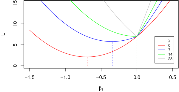
Figure 7: Lasso criterion $L$ for Example 1.

Using columns $\mathbf{Y}$ and $\mathbf{X}_{1}$ of Table 1(a) as response and explanatory variable, a regression model with parameter $\beta_{1}$ is considered. For $\lambda=0$ we have $\hat{\beta}_{1}(0)=-0.7$, located in orthant $\beta_{1}<0$, where the path starts. This is because $\sum_{i=1}^{n}x_{i1}y_{i}=-14<0$, and the Lasso path is $\hat{\beta}_{1}(\lambda)=(-14+\lambda)/20$. For increasing values of $\lambda$, $\hat{\beta}_{1}(\lambda)$ shrinks towards zero and when $\lambda\geq\left|\sum_{i=1}^{n}x_{i1}y_{i}\right|=14$, the estimate is zero. Figure 7 (Appendix) shows the criterion $L$ for this example and four values of $\lambda$. The location of the lasso estimate $\hat{\beta}_{1}$ is indicated by dashed lines.

2.2 Multiple parameters

In the unidimensional case, the parameter region was split into three orthants as $\mathbb{R}=(-\infty,0)\bigcup\{0\}\bigcup(0,\infty)$. We extend this idea with the Kronecker product of unidimensional orthants $\mathbb{R}^{p}=\bigotimes_{i=1}^{p}\mathbb{R}=\bigotimes_{i=1}^{p}\left((-\infty,0)\bigcup\{0\}\bigcup(0,\infty)\right).$ Each of the $3^{p}$ disjoint orthants is the interior of a polyhedral cone, which is identified with a vector of $p$ numbers taken from $\{\pm 1,0\}$. This vector compose the entries of a diagonal matrix of size $p$, that we refer to as $\mathbf{C}$. Using $\mathbf{C}$, vectors inside an orthant are $\mathbf{C}\mathbf{u}$, where $\mathbf{u}$ is a positive vector, that is $\mathbf{u}\in\mathbb{R}^{p}_{>0}$. The matrix $\mathbf{C}$ is central in this work, and we refer to the orthant determined by $\mathbf{C}$ as “orthant $\mathbf{C}$”.

As example, consider $\beta_{1}>0,\beta_{2}=0,\beta_{3}<0,\beta_{4}>0$. This orthant is $(0,\infty)\bigotimes\{0\}\bigotimes(-\infty,0)\bigotimes(0,\infty)=\{\mathbf{C}\mathbf{u}:\mathbf{u}\in\mathbb{R}^{4}_{>0}\}$ with $\mathbf{C}=\mbox{diag}(1,0,-1,1)$.

We refer to orthants with symbols +, -, 0 for the diagonal of $\mathbf{C}$ so that e.g. +0-+ refers to the orthant with $\mathbf{C}=\mbox{diag}(1,0,-1,1)$. We consider strict inequalities for non-zero elements so that the orthants are disjoint. If the analysis requires non-strict inequalities, this is achieved by considering all disjoint orthants involved. For example, if the desired region was $\beta_{1}\geq 0,\beta_{2}\leq 0,\beta_{3}=0$, we would consider the orthants 000, +00, 0-0 and +-0.

We formulate the parameter vector and lasso criterion over an orthant determined by matrix $\mathbf{C}$. In orthant $\mathbf{C}$, the parameter vector $\beta$ is

$$\beta=\mathbf{C}\mathbf{u},$$ (4)

with $\mathbf{u}\in\mathbb{R}^{p}_{>0}$, and the Lasso criterion of Equation (2) becomes

$$L_{\mathbf{C}}=\frac{1}{2}\mathbf{Y}^{T}\mathbf{Y}-\mathbf{u}^{T}\mathbf{C}\mathbf{X}^{T}\mathbf{Y}+\frac{1}{2}\mathbf{u}^{T}\mathbf{C}\mathbf{X}^{T}\mathbf{X}\mathbf{C}\mathbf{u}+\lambda\mathbf{u}^{T}\mathbf{C}^{2}\mathbf{1},$$ (5)

where the symbol $\mathbf{1}$ is the vector of ones of dimension $p\times 1$.

We have just turned the Lasso criterion (2) into a standard quadratic form (5) by considering orthants. The lasso penalization $||\beta||_{1}=\sum_{i=1}^{p}|\beta_{i}|$ of Equation (2) becomes $\beta^{T}\mathbf{C}\mathbf{1}=\mathbf{u}^{T}\mathbf{C}^{2}\mathbf{1}$ in (5). The quantity $\mathbf{u}^{T}\mathbf{C}^{2}\mathbf{1}$ is non-negative, as it is the sum of positive elements in $\mathbf{u}$, and $\mathbf{C}^{2}\mathbf{1}$ automatically considers zeroes as needed by the current orthant through its matrix $\mathbf{C}$. For example with +0-+0-0 we have $\mathbf{u}^{T}\mathbf{C}^{2}\mathbf{1}=u_{1}+u_{3}+u_{4}+u_{6}>0$ because the $u_{i}$ are all positive.

In orthant $\mathbf{C}$, the quadratic form $L_{\mathbf{C}}$ is well formulated because of linear independence of columns in $\mathbf{X}$. When we merge orthants, we recover $L$ over all of $\mathbb{R}^{p}$ and our development keeps the continuity and convexity properties of $L$.

2.3 Estimation of $\beta$ per orthant

We next obtain closed form solutions for the minimization of Equation (5) using standard calculus techniques. Our development gives a simple interpretation to the lasso estimates. With careful handling of the minimization solutions, we reconstruct the lasso path in Sections 3.1 and 3.2.

To minimize $L_{\mathbf{C}}$, the vector of derivatives with respect to entries in $u$ is

$$\frac{\partial L_{\mathbf{C}}}{\partial\mathbf{u}}=-\mathbf{C}\mathbf{X}^{T}\mathbf{Y}+\mathbf{C}\mathbf{X}^{T}\mathbf{X}\mathbf{C}\mathbf{u}+\lambda\mathbf{C}^{2}\mathbf{1}.$$

Although $L_{\mathbf{C}}$ is to be evaluated only with positive $\mathbf{u}$, note that $L_{\mathbf{C}}$ is a quadratic form not formally constrained to this domain, and its derivative is well defined. To determine critical points, the gradient is set to zero so that over the orthant determined by $\mathbf{C}$, the vector $\hat{\mathbf{u}}$ that minimizes $L_{\mathbf{C}}$ satisfies the linear system

$$\mathbf{C}\mathbf{X}^{T}\mathbf{X}\mathbf{C}\hat{\mathbf{u}}=\mathbf{C}\mathbf{X}^{T}\mathbf{Y}-\lambda\mathbf{C}^{2}\mathbf{1}.$$ (6)

When $\mathbf{C}$ is a full rank matrix, this is a standard linear system in $\mathbf{u}$. Depending on the number of of non-zero entries in the diagonal of $\mathbf{C}$, the system may have less than $p$ active equations, with the non-active equations becoming tautologies of the type $0=0$ with no influence on the analysis.

In what follows, we show that the active equations form a solvable, square linear system. We require a Lemma about the orthant matrix $\mathbf{C}$ and a theorem stating a property of the generalized inverse of $\mathbf{C}\mathbf{X}^{T}\mathbf{X}\mathbf{C}$. The proof of the Lemma is direct and it is not given, while the proof of the Theorem is in Appendix 1.

Lemma 1

Let $\mathbf{C}$ be a square diagonal matrix with entries from $\pm 1,0$. Then $\mathbf{C}$ equals its generalized inverse $\mathbf{C}^{-}$. Furthermore, $\mathbf{C}^{3}=\mathbf{C}$.

Theorem 2

Let $\mathbf{S}:=\mathbf{C}\mathbf{X}^{T}\mathbf{X}\mathbf{C}$, where $\mathbf{C}$ is a diagonal matrix with entries from $0,\pm 1$. The generalized inverse $\mathbf{S}^{-}$ of $\mathbf{S}$ satisfies $\mathbf{S}\mathbf{S}^{-}=\mathbf{S}^{-}\mathbf{S}=\mathbf{C}^{2}$.

Using Theorem 2, the solution of the system (6) is

$$\mathbf{C}^{2}\hat{\mathbf{u}}=\mathbf{S}^{-}\left(\mathbf{C}\mathbf{X}^{T}\mathbf{Y}-\lambda\mathbf{C}^{2}\mathbf{1}\right).$$ (7)

Equation (7) is the equation of a line with starting point $\mathbf{S}^{-}\mathbf{C}\mathbf{X}^{T}\mathbf{Y}$ and direction $-\lambda{}\mathbf{S}^{-}\mathbf{C}^{2}\mathbf{1}$, which points in the direction of maximum change of the solution. To be considered as a valid trajectory, $\mathbf{C}^{2}\hat{\mathbf{u}}$ should be positive for all its components. Not every $\mathbf{C}$ gives a valid solution, and we later describe how to determine which orthants $\mathbf{C}$ correspond to the solution of the lasso minimization.

Although the vector $\mathbf{C}^{2}\hat{\mathbf{u}}$ has dimension $p\times 1$, the non-trivial entries on it correspond to non-zero elements in the diagonal of $\mathbf{C}$, that is non zero entries in $\mathbf{C}^{2}\hat{\mathbf{u}}$ are those for which the diagonal entry in $\mathbf{C}$ is one of $\pm 1$. That is, the matrix $\mathbf{C}^{2}$ in Theorem 2 and following developments is like an identity matrix that, depending on the entries of $\mathbf{C}$, may contain some zero elements in its diagonal. An example of computation of $\mathbf{S}^{-}$ is given in Appendix 2.

The lasso estimate is obtained by left multiplying Equation (7) by $\mathbf{C}$ and using $\mathbf{C}^{3}=\mathbf{C}$ of Lemma 1, that is $\hat{\beta}=\mathbf{C}\mathbf{C}^{2}\hat{\mathbf{u}}=\mathbf{C}\hat{\mathbf{u}}$. The estimate is

$$\hat{\beta}=\mathbf{C}\mathbf{S}^{-}\mathbf{C}\left(\mathbf{X}^{T}\mathbf{Y}-\lambda\mathbf{C}\mathbf{1}\right),$$ (8)

which is composed of a linear function of observations $\mathbf{C}\mathbf{S}^{-}\mathbf{C}\mathbf{X}^{T}\mathbf{Y}$ and a biasing term $-\lambda{}\mathbf{C}\mathbf{S}^{-}\mathbf{C}^{2}\mathbf{1}$ that does not depend on observations. Because of this, the lasso estimate $\hat{\beta}$ is a nonlinear function of $\mathbf{Y}$. With orthonormal $\mathbf{X}$, $\hat{\beta}$ of Equation (8) equals the lasso estimator of Equation (3) in [1]. We use Equation (8) to evaluate $\hat{\beta}$ in a segment of the lasso path, which we show next.

Example 2

The initial lasso path of Example 1 is retrieved with Equation (8) by noting that $\mathbf{X}^{T}\mathbf{X}=20$ so $\mathbf{S}=\mathbf{C}\mathbf{X}^{T}\mathbf{X}\mathbf{C}=20$ and $\mathbf{S}^{-}=1/20$ because we are in orthant - and $\mathbf{C}=-1$. We use $\mathbf{X}^{T}\mathbf{Y}=-14$ to write $\hat{\beta}=-1/20\cdot(14-\lambda)$.

Example 3

For the data of Table 1(b) and $\lambda=0$, the least squares estimate of $\beta$ is $(-1.25,-0.3333,0.0833)^{T}$ which is the first term of Equation (8) and is the starting point of the lasso trajectory in the orthant --+. In this initial orthant, the lasso path is $\hat{\beta}=(-1.25,-0.3333,0.0833)^{T}-\lambda\cdot(-2,-1.6667,-0.3333)$.

Apart from the beginning of the path, the first term of (8) may not lie inside the orthant $\mathbf{C}$, and only when adding the second term, $\hat{\beta}$ lies in $\mathbf{C}$. This has to be checked, that is, for given $\mathbf{C},\lambda$, the coefficient $\hat{\beta}=\mathbf{C}\hat{\mathbf{u}}$ of Equation (8) will only be in its $\mathbf{C}$-orthant when all the components of $\mathbf{C}^{2}\hat{\mathbf{u}}$ of Equation (7) are non-negative. This is a consequence of our development, where we computed for positive $\mathbf{u}$ and moved back to the corresponding orthant by left multiplying by $\mathbf{C}$. The following example uses Equation (8) at an intermediate orthant in the path.

Example 4

For the data of Table 1(a), when $0.333<\lambda<1.419$, the lasso path crosses through orthant -+-. The trajectory is computed with Equation (8) yielding $\hat{\beta}=(0.1143,0.8714,-1.1857)^{T}-\lambda\cdot(0.3429,0.6143,-0.5571)^{T}$. None of two terms are in -+-, but the sum lies in this orthant over the range of $\lambda$. The trajectory is plotted in Figure 1, where solid lines show the transit of $\hat{\beta}$ through -+-. Outside the range of $\lambda$, the trajectories can still be computed, although these are not part of lasso path and are indicated with dotted lines in the figure.

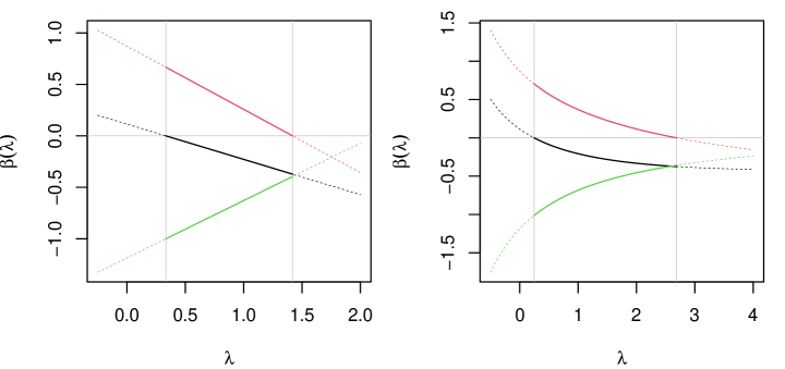
Figure 1: (left) Lasso trajectories of Example 4; (right) elastic net trajectories of Example 8. The plots also show that Equations (8) and (13) can be evaluated for $\lambda<0$. Line colors black, red and green are for $\beta_{1},\beta_{2},\beta_{3}$, respectively; grey lines indicate example values for $\lambda$ and the zero line.

In summary, Equation (8) is the explicit formula for the lasso path, but it has to be linked with a suitable orthant $\mathbf{C}$ and range for $\lambda$. The following section discusses the computation of the path relative to orthant $\mathbf{C}$ and values of $\lambda$.

3 Lasso trajectory by orthants

For a matrix $\mathbf{C}$ and a value $\lambda$, substitution of $\hat{\beta}=\mathbf{C}\hat{\mathbf{u}}$ into the criterion $L_{\mathbf{C}}$ of Equation (5) gives the smallest value of $L_{\mathbf{C}}$. This value is a polynomial function of degree two in $\lambda$ and we refer to it as $\hat{L}_{\mathbf{C}}$:

$$\hat{L}_{\mathbf{C}}=\frac{1}{2}\left(\mathbf{Y}^{T}\mathbf{Y}-\mathbf{Y}^{T}\mathbf{X}\mathbf{C}\mathbf{S}^{-}\mathbf{C}\mathbf{X}^{T}\mathbf{Y}+2\lambda\mathbf{Y}^{T}\mathbf{X}\mathbf{C}\mathbf{S}^{-}\mathbf{1}-\lambda^{2}\mathbf{1}^{T}\mathbf{S}^{-}\mathbf{1}\right).$$ (9)

This formula can be evaluated for any pair $\mathbf{C},\lambda$, but not all evaluations of $\hat{L}_{\mathbf{C}}$ will correspond to a path minimizing $L$. In what follows, we reconstruct the lasso path by first presenting an exhaustive approach and then the recommended algorithm.

3.1 All orthants lasso analysis

A simple approach to compute the estimate $\hat{\beta}(\lambda)$ at a given $\lambda$ is to evaluate $\hat{L}_{\mathbf{C}}$ over all orthants. This exhaustive method considers all cases for the diagonal of $\mathbf{C}$ from $\bigotimes_{i=1}^{p}\{-1,0,1\}=\{-1,0,1\}^{p}$ and excludes those cases of $\mathbf{C}^{2}\hat{\mathbf{u}}$ that have one or more negative entries which implies that $\hat{\beta}$ is outside the orthant determined by $\mathbf{C}$. After removing unfeasible cases, we select the orthant $\mathbf{C}$ over which $\hat{L}_{\mathbf{C}}$ of Equation (9) is minimized and retrieve the corresponding lasso estimate $\hat{\beta}$.

The analysis for a single value of $\lambda$ turns directly into the coefficients in the lasso path as follows. Set $\Lambda$ to be a collection of $\lambda$ values of interest which are positive and no larger than $\max\{|(\mathbf{X}^{T}\mathbf{Y})_{i}|,i=1,\ldots,p\}$, i.e. the value at which all the trajectories shrink to zero [1]. In the earlier expression $(\cdot)_{i}$ means the $i-$th element of the argument. For each $\lambda\in\Lambda$, select $\hat{\beta}$ associated with $\mathbf{C}$ that minimizes (9) over all orthants $\mathbf{C}$. This collection of $\hat{\beta}$ is the lasso path for $\lambda\in\Lambda$.

The exploration computes $\hat{\beta}$ and $\hat{L}_{\mathbf{C}}$ for $3^{p}$ cases of orthants $\mathbf{C}$. The advantage is that we retrieve the minimizer, but a big drawback is its cost $3^{p}\#\Lambda$, and apart from small values of $p$, we would not advise to use it in general.

3.2 Sequential lasso 1: Two types of moves

Assume that for a given $\lambda$, we are in orthant $\mathbf{C}$ and that by changing $\lambda$, we want to move to a different orthant in the path. Equation (7) suggests two possible moves available for us in the Lasso path: shrinkage and reactivation.

3.2.1 Shrinkage

Starting from orthant $\mathbf{C}$, a list of candidate $\lambda$ values for shrinking coefficients is given by those values of $\lambda$ that make the coordinates of the trajectory of Equation (7) take value zero. At $i-$th coordinate, this occurs for a value $\lambda^{*}_{i}$ computed as

$$\lambda^{*}_{i}=\frac{(\mathbf{S}^{-}\mathbf{C}\mathbf{X}^{T}\mathbf{Y})_{i}}{(\mathbf{S}^{-}\mathbf{C}^{2}\mathbf{1})_{i}}.$$ (10)

This computation is done for $i$ in $1,\ldots,p$ such that the $i-$th diagonal element of the current orthant $\mathbf{C}$ is not zero. Candidate values $\lambda^{*}_{i}$ need to be screened, as not all cases lead to valid solutions. We discard negative $\lambda_{i}^{*}$ or smaller than the current $\lambda$; those cases when the denominator $(\mathbf{S}^{-}\mathbf{C}^{2}\mathbf{1})_{i}$ is zero; and those $\lambda_{i}^{*}$ that give negative entries in the candidate solution

$$\mathbf{C}^{2}\hat{\mathbf{u}}\biggr{\rvert}_{\lambda=\lambda^{*}_{i}}=\mathbf{S}^{-}\mathbf{C}\mathbf{X}^{T}\mathbf{Y}-\frac{(\mathbf{S}^{-}\mathbf{C}\mathbf{X}^{T}\mathbf{Y})_{i}}{(\mathbf{S}^{-}\mathbf{C}^{2}\mathbf{1})_{i}}\mathbf{S}^{-}\mathbf{C}^{2}\mathbf{1}.$$

From candidates, we select the smallest positive $\lambda_{i}^{*}$ that gives non negative $\mathbf{C}^{2}\hat{\mathbf{u}}$.

Example 5

Continuing with Example 3, we determine $\lambda$ at which the lasso path moves from --+ to a neighbor orthant. Using Equation (10), we compute candidate $\lambda$ values 0.625, 0.2, -0.25 that shrink coefficients $\beta_{1},\beta_{2},\beta_{3}$, respectively. We screen candidates: the negative $\lambda$ is invalid so we are left with the first two candidates. The first $\lambda$ gives $\mathbf{C}^{2}\hat{\mathbf{u}}$ with a negative entry and it is discarded and the second candidate gives non-negative $\mathbf{C}^{2}\hat{\mathbf{u}}$ and it is selected. Thus at $\lambda=0.2$, the path moves from --+ to the neighboring orthant -0+ by shrinking $\beta_{2}$ to zero.

3.2.2 Reactivation

The majority of lasso steps involves coefficient shrinkage and the lasso path is a series of shrinkages while keeping track of increasing $\lambda$ and updating the orthant matrix $\mathbf{C}$. On occasion, a parameter that has been previously shrunk to zero becomes active, i.e. the path moves to a neighboring higher dimensional orthant.

Reactivation can only take place when some entries in the diagonal of $\mathbf{C}$ are zero. We reactivate by considering a new orthant matrix $\mathbf{C}^{\prime}$, obtained from $\mathbf{C}$ by replacing a zero entry in the diagonal by $+1$ and checking if shrinking from $\mathbf{C}^{\prime}$ gives a valid $\lambda$. This move is also done by changing the zero to $-1$ so for every zero in the diagonal of $\mathbf{C}$ we have two potential matrices $\mathbf{C}^{\prime}$. For every potential matrix $\mathbf{C}^{\prime}$, computation of candidate $\lambda$ with formula (10) is done for all coordinates non zero entries in $\mathbf{C}^{\prime}$. For a given $\mathbf{C}$, the number of neighboring orthants is $2(p-\mathbf{1}^{T}\mathbf{C}^{2}\mathbf{1})$, i.e. twice the number of zero entries in the diagonal of $\mathbf{C}$.

Example 6

Assume that the procedure is in orthant 0+-0. To reactivate, we explore neighboring higher dimensional orthants ++-0, -+-0, 0+-+ and 0+-- and see if we can reach 0+-0 by shrinking. As contrast, with direct shrink from 0+-0, we see if the lasso path moves to lower dimensional orthants 0+00 or 00-0.

Ultimately, reactivation is another shrinkage step. That is, moving from $\mathbf{C}$ to higher dimensional $\mathbf{C}^{\prime}$ is equivalent to shrinking from $\mathbf{C}^{\prime}$ to $\mathbf{C}$. Of all computations with $\mathbf{C}^{\prime}$ matrices, the smallest $\lambda$ with a valid solution is selected.

3.3 Sequential lasso 2: the algorithm

We create the lasso path by sequentially using shrinkage and reactivation. We require an algorithm for the shrinkage step, which is used in the main algorithm. We next describe both algorithms.

Algorithm 1 implements Equation (10), which is the core of the lasso procedure. In this algorithm, $\mathbf{X}$ and $\mathbf{Y}$ are the same values used in the main algorithm.

Example 5 was built with --+ for the diagonal of $\mathbf{C}$ and calling Algorithm 1 reiteratively with $i=1,2,3$. The computed $\lambda$ values of the example are those that shrink each coordinate of $\beta$ to zero. The value $\lambda_{c}$ is not given in the example so we could use $\lambda_{c}=0$ to guarantee valid shrinkage moves. When in the lasso procedure, the value $\lambda_{c}$ is passed from the main algorithm to Algorithm 1.

Input: Orthant of interest $\mathbf{C}^{\prime}$, index of coordinate to shrink the path $i$ and $\lambda_{c}$ current value of parameter $\lambda$.

Output: Candidate values $\hat{\lambda}$, $\hat{\beta}$ and criterion $\hat{L}$ corresponding to critical change in orthant $\mathbf{C}^{\prime}$ for $i$-th coordinate.

1 Compute inverse $\mathbf{S}^{-}=(\mathbf{C}^{\prime}\mathbf{X}^{T}\mathbf{X}\mathbf{C}^{\prime})^{-}$.

2If ${(\mathbf{S}^{-}\mathbf{C}^{2}\mathbf{1})_{i}}\neq 0$, compute

3$\lambda^{*}_{i}={(\mathbf{S}^{-}\mathbf{C}^{\prime}\mathbf{X}^{T}\mathbf{Y})_{i}}/{(\mathbf{S}^{-}\mathbf{C}^{2}\mathbf{1})_{i}}.$

4With $\lambda^{*}_{i}$, compute $\mathbf{C}^{\prime 2}\hat{\mathbf{u}}=\mathbf{S}^{-}\mathbf{C}^{\prime}\mathbf{X}^{T}\mathbf{Y}-\lambda^{*}_{i}\mathbf{S}^{-}\mathbf{C}^{2}\mathbf{1}$, $\hat{\beta}=\mathbf{C}^{\prime}\hat{\mathbf{u}}$ and $\hat{L}_{C^{\prime}}$.

5If ${(\mathbf{S}^{-}\mathbf{1})_{i}}=0$, or if there are negative entries in $\mathbf{C}^{\prime 2}\hat{\mathbf{u}}$, or if $\lambda^{*}_{i}\leq\lambda_{c}$ then set output $RES:=\{\}$, otherwise set $RES:=\{\hat{\lambda}:=\lambda^{*}_{i},\hat{\beta},\hat{L}:=\hat{L}_{C^{\prime}}\}.$

Return $RES$.

Algorithm 1 Shrinkage step for $i$-th coordinate

Algorithm 2 is our main procedure. The algorithm builds the path from the ordinary least squares estimate and proceeds by a series of shrinkage and reactivation movements. At a given step in the path, the algorithm explores neighboring orthants and moves in the direction of steepest descent determined by the smallest valid candidate $\lambda$ in step 2. Because this move is in the lasso path, the quantity $L^{*}$ which was computed as $\hat{L}_{\mathbf{C}}$ is the minimal value of criterion $L$ at $\lambda=\lambda^{*}$.

Algorithm 2 is guaranteed to always terminate because, in the worst case scenario, it will visit the complete list of all orthants, which is finite. In practice, the algorithm only visits a subset of all orthants.

Input: Design model matrix $X$ with $p$ columns, vector of observations $Y$.

Output: Lasso path with $\lambda$, $\beta(\lambda)$ and $L$ at path breakpoints.

1 Initialization: Compute $\hat{\beta}=(\mathbf{X}^{T}\mathbf{X})^{-1}\mathbf{X}^{T}\mathbf{Y}$. Set matrix $\mathbf{C}:=\mbox{diag}(\operatorname{sign}(\hat{\beta}))$; compute $\hat{L}_{\mathbf{C}}$; set $\lambda:=0$ and output $O:=\{\{\ \lambda,\hat{\beta},\hat{L}_{\mathbf{C}}\}\}$.

2while $\mathbf{C}\neq\mathbf{0}$ do

3      

4      for $j\in\{1,\ldots,p\}$ do

5             if $C_{j,j}=0$ then

6                   for $k\in\{-1,1\}$ do

7                        

8                        Set $\mathbf{C}^{\prime}:=\mathbf{C}$ and update $C^{\prime}_{j,j}:=k$.

9                        for $i\in\{1,\ldots,p\mbox{ such that }C^{\prime}_{i,i}\neq 0\}$ do

10                               Run Algorithm 1 with inputs $\mathbf{C}^{\prime},i,\lambda_{c}:=\lambda$. Nonempty outputs $\{\hat{\lambda}$, $\hat{\beta}$ and $\hat{L}\}$ are kept until used in Step 2.

11                         end for

12                        

13                   end for

14                  

15            else

16                   Set $\mathbf{C}^{\prime}:=\mathbf{C}$.

17                  Run Algorithm 1 with inputs $C^{\prime},i:=j,\lambda_{c}:=\lambda$. Nonempty outputs $\{\hat{\lambda}$, $\hat{\beta}$ and $\hat{L}\}$ are kept until used in Step 2.

18             end if

19            

20       end for

21      

22      From the set of all nonempty outputs $\{\{\hat{\lambda},\hat{\beta},\hat{L}\}\}$ of the loop in steps 2-2, select the smallest $\hat{\lambda}$. Call this $\lambda^{*}$, with associated $\beta^{*},L^{*}$.

23      Update output $O$ with these values, i.e. $O:=O\cup\{\lambda^{*},\beta^{*},L^{*}\}$.

24      Update $\lambda:=\lambda^{*}$ and $\mathbf{C}:=\mbox{diag}(\operatorname{sign}(\beta^{*}))$.

25 end while

26

Algorithm 2 Orthant lasso

3.4 Detailed lasso example

The lasso path we describe uses the data of Table 1(a) and was selected because it requires a reactivation step despite its small size. The path has initial shrinkage, reactivation of a variable and a final series of shrinkage steps. In Appendix 3 we detail the moves of the algorithm as the path traverses through orthants.

Table 2(a) summarizes the breakpoints of the lasso path for this example. Each row lists $\lambda$, vector of coefficients $\beta$ and criterion $L$ at a breakpoint of the path. The list of orthants involved in the path is ++-, 0+-, -+-, -0-, -00, 000, which can be seen from right to left in the standard plot of the lasso path of Figure 2(a). Table 3 in Appendix 3 details all moves for this example. The table should be read from the top, as rejection of candidates $\hat{\lambda}$ depends on the current value of $\lambda$.

Figure 3(a) shows criterion $L$ as a function of $\lambda$ along the path, i.e. we plot $\hat{L}_{\mathbf{C}}$ for the orthants in the path. Colors indicate orthants, with bold line when the lasso path traverses along the orthant and $\hat{L}_{\mathbf{C}}$ becomes $L$, and with thin line when $\hat{L}_{\mathbf{C}}$ is not in the path. Finally, Figure 6 in the Appendix shows potential lasso moves after exhaustive orthant exploration and rejection of unsuitable moves.

Lasso	Elastic net
$\begin{array}[]{l|rrr|l}\hline\cr\lambda&\vrule\lx@intercol\hfil\beta\hfil\lx@intercol\vrule\lx@intercol&L\\ \hline\cr 0&0.114&0.871&-1.186&0.843\\ 0.118&0&0.735&-1.029&1.074\\ 0.333&0&0.667&-1&1.444\\ 1.419&-0.372&0&-0.395&2.765\\ 5.429&-0.429&0&0&5.163\\ 14&0&0&0&7\\ \hline\cr\end{array}$	$\begin{array}[]{l|rrr|l}\hline\cr\lambda&\vrule\lx@intercol\hfil\beta\hfil\lx@intercol\vrule\lx@intercol&E\\ \hline\cr 0&0.114&0.871&-1.186&0.843\\ 0.146&0&0.732&-1.026&1.054\\ 0.247&0&0.704&-1.013&1.181\\ 2.687&-0.374&0&-0.359&2.898\\ 16.961&-0.194&0&0&6.465\\ 28&0&0&0&7\\ \hline\cr\end{array}$
(a)	(b)

Table 2: (a) Lasso path of the example of Section 3.4 and (b) Elastic net path for the same data and $\alpha=0.5$, see Example 9.

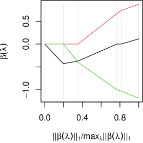
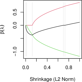
(a)	(b)
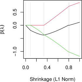
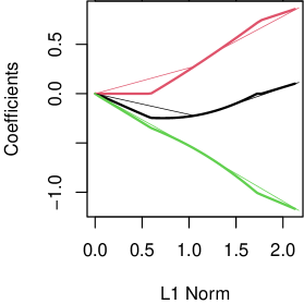
(c)	(d)

Figure 2: Shrinkage results of Table 1(a) data. Panel (a) has Lasso of Table 2(a); panels (b) and (c) have the elastic net of Table 2(b). Panel (d) has glmnet results, further described in Example 12. The colors black, red, green in the plots correspond to trajectories of coefficients $\beta_{1},\beta_{2},\beta_{3}$, respectively.

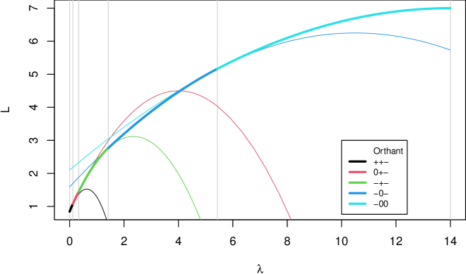
(a)

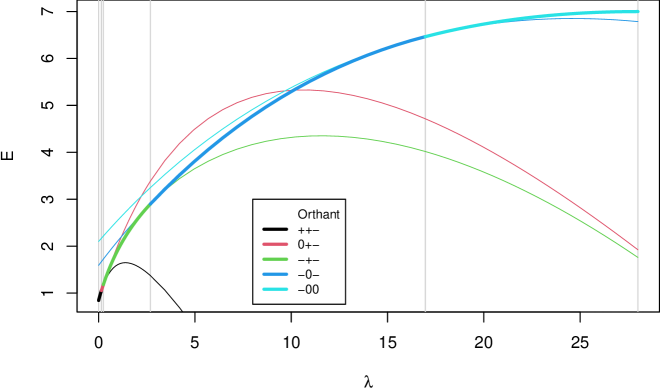
(b)

Figure 3: (a) Criterion $L$ of Lasso as the path moves along orthants. Panel (b) has $E$ of elastic net with $\alpha=0.5$. Both cases use data in Table 1(a).

4 Elastic net

Elastic net regularization combines model selection of lasso with improved prediction features of $L_{2}$ penalization. The criterion to be minimized is $E$ of Equation (3) in Section 1.2. The nonnegative $\lambda$ controls the parameter penalization relative to residual sum of squares; while $\alpha$ is a fixed number in $(0,1]$ that balances between the penalization $||\beta||_{1}$ of lasso, achieved when $\alpha=1$ and the quadratic penalty $||\beta||_{2}^{2}$ used in ridge regression and reached when $\alpha\to 0$. We exclude $\alpha=0$ because at that point there is no shrinkage to zero for finite $\lambda$.

Elastic net [12] has been shown to improve over lasso when predictors are heavily correlated [10]. Lasso methods can be used in estimation of elastic net [12], and an implementation of the elastic net using coordinate descent is the R library glmnet, see [10]. A recent version of the elastic net criterion uses s-estimators to improve estimation and variable selection performance under heavy tailed error distributions [13]. We next develop the orthant to estimation in elastic nets.

4.1 Elastic net by orthants

The orthant development for the elastic net mirrors what was done earlier for lasso, setting $\beta=\mathbf{C}\mathbf{u}$ so that over the orthant determined by $\mathbf{C}$ the criterion is

$$E_{\mathbf{C}}=\frac{1}{2}\mathbf{Y}^{T}\mathbf{Y}-\mathbf{u}^{T}\mathbf{C}\mathbf{X}^{T}\mathbf{Y}+\frac{1}{2}\mathbf{u}^{T}\mathbf{C}\mathbf{X}^{T}\mathbf{X}\mathbf{C}\mathbf{u}+\lambda\alpha\mathbf{u}^{T}\mathbf{C}^{2}\mathbf{1}+\lambda\frac{1-\alpha}{2}\mathbf{u}^{T}\mathbf{C}^{2}\mathbf{u}.$$ (11)

The entries of vector $\mathbf{u}$ are required to be positive, although there is no mathematical restriction for the entries of $\mathbf{u}$, which can be real numbers. In other words, $E_{\mathbf{C}}$ is a well formulated quadratic form, which was also the case for $L_{\mathbf{C}}$.

The solution to the minimization of $E_{\mathbf{C}}$ is the system

$$\left(\mathbf{C}\mathbf{X}^{T}\mathbf{X}\mathbf{C}+\lambda(1-\alpha)\mathbf{C}^{2}\right)\mathbf{u}=\mathbf{C}\mathbf{X}^{T}\mathbf{Y}-\lambda\alpha\mathbf{C}^{2}\mathbf{1}.$$

The matrix $\mathbf{C}\mathbf{X}^{T}\mathbf{X}\mathbf{C}+\lambda(1-\alpha)\mathbf{C}^{2}$ is the orthant counterpart of regularising $\mathbf{X}^{T}\mathbf{X}$ with a multiple of the identity matrix in ridge regression, also known as Tikhonov’s regularization. The next theorem gives a property of the generalized inverse of this matrix. We omit its proof, which is similar to that of Theorem 2.

Theorem 3

Let $\mathbf{S}(\lambda):=\mathbf{C}\mathbf{X}^{T}\mathbf{X}\mathbf{C}+\lambda(1-\alpha)\mathbf{C}^{2}$ and let $\mathbf{S}(\lambda)^{-}$ be its generalized inverse. Then $\mathbf{S}(\lambda)^{-}$ satisfies $\mathbf{S}(\lambda)\mathbf{S}(\lambda)^{-}=\mathbf{S}(\lambda)^{-}\mathbf{S}(\lambda)=\mathbf{C}^{2}$.

Using Theorem 3, we have the solution

$$\mathbf{C}^{2}\hat{\mathbf{u}}=\mathbf{S}(\lambda)^{-}\left(\mathbf{C}\mathbf{X}^{T}\mathbf{Y}-\alpha\lambda{}\mathbf{C}^{2}\mathbf{1}\right)$$ (12)

and by using $\hat{\beta}=\mathbf{C}\hat{\mathbf{u}}$, retrieve the elastic net estimate

$$\hat{\beta}=\mathbf{C}\mathbf{S}(\lambda)^{-}\mathbf{C}\left(\mathbf{X}^{T}\mathbf{Y}-\alpha\lambda{}\mathbf{C}\mathbf{1}\right).$$ (13)

The elastic net trajectory $\hat{\beta}$ starts from the ridge estimate $\mathbf{C}\mathbf{S}(\lambda)^{-}\mathbf{C}\mathbf{X}^{T}\mathbf{Y}$ and moves in the direction $-\alpha{}\lambda{}\mathbf{C}\mathbf{S}(\lambda)^{-}\mathbf{C}^{2}\mathbf{1}$. This trajectory minimizes $E_{\mathbf{C}}$ over the orthant determined by $\mathbf{C}$, in other words, it is the exact elastic net path with no approximations involved. When formulated as a naïve elastic net, $\hat{\beta}$ of Equation (13) coincides with estimator for orthonormal $\mathbf{X}$ of Equation (6) in [12].

The notation $\mathbf{S}(\lambda)$ in Theorem 3 and elsewhere emphasizes the main role of $\lambda$: although $\mathbf{S}(\lambda)$ depends on $\alpha$ and $\lambda$, in analyses $\alpha$ is kept fixed. We give an example of computation of $\mathbf{S}(\lambda)^{-}$ in Appendix 2.

Given the dependence of direction of descent on $\lambda$ through the matrix $\mathbf{S}(\lambda)^{-}$, the trajectories of net coefficients are not piecewise linear functions of $\lambda$ as with lasso. The following example shows nonlinearity of $\hat{\beta}$ even for a single explanatory variable. Example 8 shows computation of $\hat{\beta}$ for a given orthant and range of $\lambda$.

Example 7

Consider data of Table 1(a) with single explanatory variable $\mathbf{X}_{1}$ as in Examples 1 and 2. The least squares estimator $\hat{\beta}=-0.7$ lies in orthant - so $C=-1$. Using $\mathbf{X}^{T}\mathbf{X}=20$, the generalized inverse $\mathbf{S}(\lambda)^{-}$ is the scalar $\left(20+\lambda(1-\alpha)\right)^{-1}$, and the net path is $\hat{\beta}=C\hat{\mathbf{u}}=-1/\left(20+\lambda(1-\alpha)\right)\cdot\left(14-\alpha\lambda\right),$ where we used $\mathbf{X}^{T}\mathbf{Y}=-14$. By substituting $\alpha=1$ in the net path $\hat{\beta}$, we retrieve the lasso estimate of Example 1.

Example 8

In Figure 1 (right) we give part of the elastic net path for analysis of Table 2(b). This segment is computed with Equation (13) and orthant -+-, that corresponds to the path between rows $3$ and $4$ of the table. The trajectories are shown in solid line as they cut through -+- for $\lambda\in(0.247,2.687)$, and in dashed line outside the stated range of $\lambda$ at which point the trajectories are outside -+-.

For given $\lambda$ and $\mathbf{C}$, by substituting $\hat{\beta}=\mathbf{C}\hat{\mathbf{u}}$ of Equation (13) into $E_{\mathbf{C}}$ of Equation (11), we obtain the smallest value of elastic net criterion $E_{\mathbf{C}}$. This is a nonlinear function of $\lambda$ and $\alpha$ with the following expression

$$\hat{E}_{\mathbf{C}}=\frac{1}{2}\Big{(} \mathbf{Y}^{T}\mathbf{Y}-\mathbf{Y}^{T}\mathbf{X}\mathbf{C}\mathbf{S}(\lambda)^{-}\mathbf{C}\mathbf{X}^{T}\mathbf{Y}-2\lambda\alpha\mathbf{1}^{T}\mathbf{S}(\lambda)^{-}\mathbf{C}\mathbf{X}^{T}\mathbf{Y}-\lambda^{2}\alpha^{2}\mathbf{1}^{T}\mathbf{S}(\lambda)^{-}\mathbf{1}$$

$$+\lambda(1-\alpha)\mathbf{Y}^{T}\mathbf{X}\mathbf{C}\mathbf{S}(\lambda)^{-}\mathbf{S}(\lambda)^{-}\mathbf{C}\mathbf{X}^{T}\mathbf{Y}-2\lambda^{2}\alpha\mathbf{1}^{T}\mathbf{S}(\lambda)^{-}\mathbf{S}(\lambda)^{-}\mathbf{C}\mathbf{X}^{T}\mathbf{Y}$$

$$+\lambda^{3}\alpha^{2}(1-\alpha)+\mathbf{1}^{T}\mathbf{S}(\lambda)^{-}\mathbf{S}(\lambda)^{-}\mathbf{1} \Big{)}.$$

4.2 All orthants net analysis

The all orthant approach of Section 3.1 can be applied with little change to the elastic net, i.e. for a given $\lambda$, consider all orthants and select the $\hat{\beta}$ that minimizes $\hat{E}_{\mathbf{C}}$. The same screening considerations for orthant lasso must be used: discard those cases for which $\mathbf{C}^{2}\hat{\mathbf{u}}$ has negative entries, equivalently discard when $\hat{\beta}$ is not in orthant $\mathbf{C}$. All orthant computations can be done for a collection $\Lambda$ of values of $\lambda$ and has exponential cost, akin to the situation described in Section 3.1.

4.3 Sequential approach to elastic net

With a minor change, Algorithm 2 can be applied to the computation of the elastic net path. Consider an elastic net path in orthant $\mathbf{C}$. We find a breakpoint for changing orthants for the $i$-th coordinate by solving $(\mathbf{C}^{2}\hat{\mathbf{u}})_{i}=0$, i.e.

$$(\mathbf{S}(\lambda)^{-}\mathbf{C}\mathbf{X}^{T}\mathbf{Y})_{i}-\alpha\lambda({}\mathbf{S}(\lambda)^{-}\mathbf{C}^{2}\mathbf{1})_{i}=0,$$ (14)

which has to be solved for $\lambda$. Rearranging this expression leads to

$$\lambda_{i}^{*}=\frac{(\mathbf{S}(\lambda_{i}^{*})^{-}\mathbf{C}\mathbf{X}^{T}\mathbf{Y})_{i}}{\alpha(\mathbf{S}(\lambda_{i}^{*})^{-}\mathbf{C}^{2}\mathbf{1})_{i}},$$ (15)

which generalizes Equation (10) and depends on $\lambda^{*}_{i}$ on both sides. The modification of Step 1 in Algorithm 1 is to solve numerically Equation (14), that is

3 Solve $(\mathbf{S}(\lambda)^{-}\mathbf{C}\mathbf{X}^{T}\mathbf{Y})_{i}-\alpha\lambda({}\mathbf{S}(\lambda)^{-}\mathbf{C}^{2}\mathbf{1})_{i}=0$ for $\lambda$ and call $\lambda_{i}^{*}$ to the solution.

We give two examples of elastic net computation, and in sections 5.2 and 5.3 we discuss our implementation and compare against glmnet.

Example 9

An elastic net with $\alpha=0.5$ was fitted to data of Example 1(a) using Algorithms 1 and 2 with the adaptation discussed above. Table 2(b) shows the breakpoints at which the elastic net path changes orthant. The coefficients $\hat{\beta}$ are not piecewise linear functions of $\lambda$, however they are computed easily using Equation (13) with the appropriate orthant $C$. In Figure 2 panels (b) and (c) we show the elastic net path, and in Figure 3(b) we show the evolution of criterion $E$ as it crosses orthants of the elastic net path in its shrinking route towards zero.

Example 10

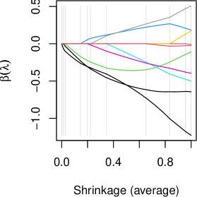
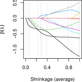
(a)	(b)

Figure 8: (a) and (b) elastic net paths for synthetic data and $\alpha$ values $0.4$ and $0.8$, respectively. The horizontal shrinkage in the plots is the average of $L_{1}$ and $L_{2}$ norms.

Figure 8 (Appendix) shows elastic net path fits for a synthetic dataset of $n=12$ observations in $p=10$ variables. Two values of $\alpha$ were used for the analysis and in both cases, the steps in the net trajectory were only shrinkage steps.

The criterion of elastic net can be studied plotting $E$ against the shrinkage parameter $\lambda$. Figure 3(b) shows the evolution of piecewise nonlinear criterion $E$ for the data of Example 9. Line colors indicate orthants in the path, with bold whenever the net path is traversing the orthant and thin line for suboptimal curves, that is when the elastic net path is in another orthant.

5 Conclusions and further discussion

We have presented a new orthant method for the computation of lasso and elastic net estimates. Our proposal uses simple calculus techniques and gives exact results. We proposed an algorithm to build the path that avoids expensive orthant evaluation and that has worked well in the examples we tried. We briefly elaborate on issues still pending concerning implementation and theory development.

5.1 Lasso computations and implementation

The algorithm for lasso by orthants requires the iterative solution of Equation (7) for the $i$-th component. This is a linear equation whose explicit solution is Equation (10) that has proved to be remarkably stable. A prototype R implementation lassoq of our algorithm for lasso path is given in Appendix 4 of this paper.

Our code gives mostly the same results as the lars implementation of lasso [11], although on some instances, it improves over it as in the following example.

Example 11

For the data of Table 1(b) and for $0<\lambda<0.0833$, lars gives the lasso path as $(-1.25,-0.3333,0.0833)^{T}-\lambda\cdot(0,1,1)^{T}$. This path makes the $L_{1}$ norm of $\hat{\beta}$ a constant in --+ and is not in the direction of maximum descent. The orthant computation with the same data and initial lasso step of Example 3 gives a trajectory in the direction of maximum descent.

5.2 Solving the orthant net equation

The elastic net path by orthants requires solving Equation (14), i.e. finding $\lambda$ for which the $i$-th component of $\mathbf{C}^{2}\hat{\mathbf{u}}$ is zero. In essence, this is solving a univariate non-linear equation and we survey classical approaches to this problem.

Simple iteration of Equation (15) starts from initial $\lambda_{0}$ and for $j=1,2,\ldots$ computes $\lambda_{j}={(\mathbf{S}(\lambda_{j-1})^{-}\mathbf{C}\mathbf{X}^{T}\mathbf{Y})_{i}}/{\left(\alpha(\mathbf{S}(\lambda_{j-1})^{-}\mathbf{C}^{2}\mathbf{1})_{i}\right)}.$ Another possibility is Newton’s method that iterates $\lambda_{j}=\lambda_{j-1}-(\mathbf{C}^{2}\hat{\mathbf{u}})_{i}/(\mathbf{S}(\lambda_{j-1})^{-}((1-\alpha)\mathbf{C}^{2}\hat{\mathbf{u}}-\alpha\mathbf{1}))_{i}$, where $\mathbf{C}^{2}\hat{\mathbf{u}}$ also depends on $\lambda_{j-1}$. In either approach, iteration continues until the absolute difference between values $|\lambda_{j}-\lambda_{j-1}|$ is within a specified threshold. In our experience, these two iteration methods can lead in some cases, to $\lambda_{j}$ oscillating outside the allowable range $[0,\max_{i}|(X^{T}Y)_{i}|/\alpha]$ and have not pursued its use.

We have experimented with two other iterative methods that have proved more stable in our numerical examples. One is the secant method, that does not require derivative information, and the other is the bisection method. The latter method, although it is not the most efficient, is the method that has worked best for the orthant net method. We are exploring ways to improve the numerical stability and accuracy of numerical solvers. This is work in progress, for which we have a prototype R implementation elastiq given in Appendix 5 of this paper.

5.3 Implementation of elastic net

We look at results obtained with the orthant net method and those of the R package glmnet. This function regularizes generalized linear models, and we use the option family=gaussian. Our comparison is not about the speed of computations nor about the dimensionality of data, but about the quality of results obtained.

We emphasize that results obtained with the orthant net method are not approximations but are exact solutions to the minimization of criterion $E$. In contrast, glmnet appears designed not for precise results but for fast approximate analysis. We compare net methods through examples and discuss a simulation.

Example 12

Two glmnet analyses were carried out with the data of Table 1(a) and $\alpha=0.5$: one analysis without supplying $\lambda$ values and another uses $\lambda$ breakpoints from the orthant net of Table2(b). Both results are shown in Figure 2(d), where bold lines are for the first analysis and thin lines are for the second analysis.

We compare results with orthant net results of Figure 2(c). When $\lambda$ is not supplied in glmnet, the patterns of $\beta_{1},\beta_{2}$ are similar to the exact orthant values. However, the shrinkage pattern of $\beta_{3}$ is not correctly recovered and this parameter shrinks to zero later than should be. When $\lambda$ breakpoints are supplied, glmnet analysis produces trajectories that differ substantially from the orthant solution, with $\beta_{2},\beta_{3}$ shrinking later than needed. It is also surprising that even the least squares estimate from glmnet for both cases only agrees with the correct value when rounded to a single digit.

As for orthants covered, glmnet generally recovers less orthants than the correct orthant solution. The elastic net orthant solution of Table 2(b) goes through orthants ++-, 0+-, -+-, -0-, -00, 000. Without specifying $\lambda$, the glmnet path traverses through less orthants ++-, 0+-, -+-, -0-, 000, and finally, when specifying $\lambda$ breakpoints, the glmnet path only crosses the orthants ++-, -+-, 000.

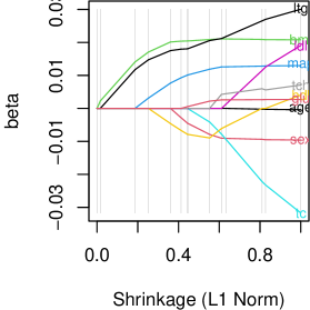
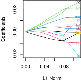
(a)	(b)

Figure 4: Analysis of scaled diabetes data with (a) the elastic net orthant of this paper and (b) glmnet.

Example 13

We carried out elastic net orthant and glmnet analyses for synthetic data. Both analyses used $\alpha=0.5$ and glmnet was used without specifying $\lambda$. Default glmnet analysis does $93$ steps with redundancy as they only cover $40$ orthants, while the net orthant method yields $56$ steps with no redundant orthants retrieved. The orthants visited with each methodology are given in Figure 10 (Appendix). The glmnet agrees with $55.4\%$ of the orthants of the net orthant approach.

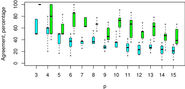
Figure 5: Agreement between orthant method and glmnet for simulated data. In green, agreement between orthant and glmnet analysis without specifying $\lambda$; in light blue, agreement when glmnet uses $\lambda$ provided by the orthant. The horizontal axis is the dimension $p$.

Example 14

An elastic net analysis of the diabetes data set [1] with $\alpha=0.5$ was performed. Two methods were used: elastic net orthant and glmnet without specifying $\lambda$. The data for both analyses was scaled by a constant $k=25000$. This scaling was used to stabilize the elastic net orthant computation. Figure 4 shows the paths for both analyses, and despite some similarities, glmnet tends to collapse most trajectories at a single step of the trajectory, contrary to the orthant method in which the trajectories shrink to zero at different points in the path. Figure 9 (Appendix) shows orthant traverses for each method. The glmnet path has an agreement of only $20\%$ with the orthant method.

The examples suggest that glmnet results may differ with the orthant net method and we compared with simulation experiment. We simulated data with dimensions $p$ from $3$ to $15$, for each dimension simulating $42$ data sets. For each set we fitted elastic net using the orthant method as well as glmnet, using $\alpha$ from $0.3$ to $0.9$. We recorded the orthants visited by every method, and computed the percentage of glmnet orthants that agree with the orthant net method. Two versions of glmnet were compared: without providing $\lambda$ and using breakpoints from the orthant net method. The agreement decreases with increasing $p$; and the agreement is lower when we provide breakpoint values of $\lambda$, see Figure 5. There is not much change of agreement as function of $\alpha$ (plot not shown).

5.4 Further work

Orthant work can be extended in several directions. Firstly, expectation of Equation (8) for lasso or (13) for elastic net allows exact bias computation which could be used to compare results under model misspecification. This analysis is contingent on choice of $\lambda$ and $\mathbf{C}$, and theory developments should consider ways of removing this dependence from bias results.

A second line of work is the comparison of our algorithm with the modified LARS algorithm [3] used to compute lasso. By construction, our proposal already gives the optimal path, but we still have to study the equivalence against the LARS algorithm, which we have already pointed that has substandard performance in some instances. A related development is the removal of the reactivation step in Algorithm 2. This would make orthant computations much faster and should be compared with the unmodified LARS algorithm.

A modified approach to lasso considers constraints on parameters to achieve polynomial hierarchy along the path [14], generalizing hierarchical lasso work by [15]. The constrained approach to the path is carried out by numerical minimization over cones, with no apparent closed formulæ available. Two possibilities arise here. One is the development over the cones themselves, while would be to project the path into the constrained region to create an approximate constrained path which would be compared with the correct lasso or elastic net paths.

Orthant methods can be adapted to different ways of regularizing. A direct case is the naïve elastic net with penalty $\lambda_{1}||\beta||_{1}+\lambda_{2}||\beta||_{2}^{2}/2$, implemented in LassoNet, see [16, 17]; or adaptive lasso [18] in which coefficients are weighed in the penalty function $\sum_{j=1}^{p}w_{j}|\beta_{j}|$. In both cases the orthant approach can be used, see an example of adaptive lasso in Appendix 6. However, fused lasso [19] with penalty $\lambda_{1}||\beta||_{1}+\lambda_{2}\sum_{j=2}^{n}|\beta_{j}-\beta_{j-1}|$ and the penalty $\lambda||\mathbf{D}\beta||_{1}$ of generalized lasso [4] would require careful consideration. These two latter cases are still quadratic forms, not defined over orthants, but rather over polyhedral cones. The computation of $\lambda$ breakpoints should consider entry and exit points of paths between cones.

Appendixes

Appendix 1 - Proof of Theorem 2

Proof. The proof is by construction. Without lack of generality, we assume that all non-zero entries in the diagonal of $\mathbf{C}$ take value one, and to avoid a trivial case, there is at least one non-zero entry in the diagonal of $\mathbf{C}$.

The matrix $\mathbf{X}\mathbf{C}$ has the same size as $\mathbf{X}$, but with some columns of $\mathbf{X}$ replaced by zero columns. The matrix $\mathbf{S}=\mathbf{C}\mathbf{X}^{T}\mathbf{X}\mathbf{C}$ is the same size as $\mathbf{X}^{T}\mathbf{X}$ and its contents are equal those of $\mathbf{X}^{T}\mathbf{X}$ except for some zero rows and columns. The location of the zero columns of $\mathbf{X}\mathbf{C}$ and the zero rows and columns of $\mathbf{S}$ corresponds to the zeroes in the diagonal of $\mathbf{C}$. The rank of $\mathbf{X}\mathbf{C}$ equals the number of non-zero entries in the diagonal of $\mathbf{C}$, because the non-zero columns of $\mathbf{X}\mathbf{C}$ are linearly independent. The non-zero submatrix of $\mathbf{C}\mathbf{X}^{T}\mathbf{X}\mathbf{C}$ has also the same rank as $\mathbf{X}\mathbf{C}$ and is invertible. The inverse $\mathbf{S}^{-}$ is the ordinary matrix inverse of the non-zero submatrix of $\mathbf{S}$, located according to non-zero entries in the diagonal of $\mathbf{C}$.

If $\mathbf{C}$ is full rank, then $\mathbf{C}=\mathbf{I}$ and the inverse is $\mathbf{S}^{-}=\mathbf{S}^{-1}$ so that $\mathbf{S}\mathbf{S}^{-}=\mathbf{I}=\mathbf{C}^{2}$. In general, when we multiply $\mathbf{S}\mathbf{S}^{-}$, we are doing the product of the smaller, nonzero invertible submatrix of $\mathbf{C}\mathbf{X}^{T}\mathbf{X}\mathbf{C}$ with its inverse, hence we always obtain an submatrix of the identity which is precisely $\mathbf{C}^{2}$, that is $\mathbf{S}\mathbf{S}^{-}=\mathbf{C}^{2}$ which has ones in the positions of non-zero entries in the diagonal of $\mathbf{C}$. A similar argument is used to show that $\mathbf{S}^{-}\mathbf{S}=\mathbf{C}^{2}$.

In the case of non-zero entries of $\mathbf{C}$ taking value $-1$, the development described holds because the rank of both $\mathbf{X}\mathbf{C}$ and $\mathbf{S}$ is not altered by some columns of $\mathbf{X}\mathbf{C}$ reversing sign and for some sign changes in columns and rows of $\mathbf{S}$.

The construction gives a unique matrix $\mathbf{S}^{-}$ which is a Moore-Penrose inverse as it satisfies $\mathbf{S}\mathbf{S}^{-}\mathbf{S}=\mathbf{S}$, $\mathbf{S}^{-}\mathbf{S}\mathbf{S}^{-}=\mathbf{S}^{-}$ and both $\mathbf{S}^{-}\mathbf{S}$ and $\mathbf{S}\mathbf{S}^{-}$ are diagonal.   

Theorem 2 is still valid for the trivial case in the last step of lasso when $\mathbf{C}$ has all zeroes in its diagonal in which case $\mathbf{S}^{-}=\mathbf{C}$. The proof for Theorem 3 follows the rationale above as $\mathbf{S}(\lambda)=\mathbf{C}\mathbf{X}^{T}\mathbf{X}\mathbf{C}+\lambda(1-\alpha)\mathbf{C}^{2}$ involves a submatrix of $\mathbf{X}^{T}\mathbf{X}$ regularized with a multiple of identity with corresponding dimensions.

Appendix 2 - Examples of $\mathbf{S}^{-}$ and $\mathbf{S}(\lambda)^{-}$

We give one example of the computation of the inverse $\mathbf{S}^{-}$ and another of $\mathbf{S}(\lambda)^{-}$. Both examples use the matrix $\mathbf{X}$ of Table 1(a).

Example 15

Consider the orthant 0+-, i.e. the matrix $\mathbf{C}$ has diagonal entries $0,1,-1$ and for computations we only use the columns $2,3$ of $\mathbf{X}$. The inverse $\mathbf{S}^{-}$ is built with the usual inverse of the lower $2\times 2$ block. We have

$$\mathbf{S}=\left(\begin{array}[]{rrr}0&0&0\\ 0&4&-2\\ 0&-2&12\\ \end{array}\right),\;\;\mathbf{S}^{-}=\frac{1}{44}\left(\begin{array}[]{rrr}0&0&0\\ 0&12&2\\ 0&2&4\\ \end{array}\right)\mbox{ and }\mathbf{S}\mathbf{S}^{-}=\left(\begin{array}[]{rrr}0&0&0\\ 0&1&0\\ 0&0&1\\ \end{array}\right).$$

Example 16

Consider $\mathbf{C}$ of orthant -0-. For $\lambda=10$ and $\alpha=0.5$ we have

$$\mathbf{S}(\lambda)=\left(\begin{array}[]{rrr}25&0&13\\ 0&0&0\\ 13&0&17\\ \end{array}\right),\;\;\mathbf{S}(\lambda)^{-}=\frac{1}{256}\left(\begin{array}[]{rrr}17&0&-13\\ 0&0&0\\ -13&0&25\\ \end{array}\right)\mbox{ and }\mathbf{S}(\lambda)\mathbf{S}(\lambda)^{-}=\left(\begin{array}[]{rrr}1&0&0\\ 0&0&0\\ 0&0&1\\ \end{array}\right).$$

Appendix 3 - Orthant moves for Section 3.4

We detail the algorithm moves for the data of Table 1(a).

1. Initialization

   The least squares estimate is $\hat{\beta}=(0.114,0.871,-1.186)^{T}$. We have orthant ++-; compute $L=0.843$ and set $\lambda=0$.

2. Current orthant ++- with $\lambda=0$

   Matrix $\mathbf{C}$ has no zero elements in its diagonal so no reactivation is done. We proceed to shrink every coordinate using Algorithm 1 with $i=1,2,3$.

   Of the candidate $\hat{\lambda}$, only $\lambda^{*}=0.118$ is valid and we have $\beta^{*}=(0,0.735,-1.029)^{T}$; criterion $L=1.074$ and update the orthant to 0+-.

3. Current orthant 0+- with $\lambda=0.118$

   The diagonal of $\mathbf{C}$ has a zero and we reactivate, i.e. substitute $C_{1,1}$ with each of $\mp 1$. Using $-1$ leads to orthant -+-, and shrinking from this orthant gives two valid candidates $\hat{\lambda}$. Reactivating with $+1$ creates orthant ++-, and shrinking from ++- repeats the computation of step 2 above, only this time there are no valid $\hat{\lambda}$ candidates because of the current value $\lambda=0.118$.

   Shrinking from 0+- with $i=2,3$ gives two $\hat{\lambda}$, of which only one is valid.

   We have three valid $\hat{\lambda}$ candidates. We select $\lambda^{*}=0.333$ with $\beta^{*}=(0,0.667,-1)^{T}$ and criterion $L=1.444$. We remain in orthant 0+- because of $\beta^{*}$.

4. Current orthant 0+- with $\lambda=0.333$

   The moves are a second pass of what was already done in step 3: reactivation to -+- and ++-; shrinkage from 0+-. Given the current value of $\lambda$, one earlier candidate from step 3 is not valid and we have two valid $\hat{\lambda}$ candidates.

   We select $\lambda^{*}=1.419$ with parameter vector $\beta^{*}=(-0.372,0,-0.395)^{T}$, criterion $L=2.765$ and update orthant to -0-.

5. Current orthant -0- with $\lambda=1.419$

   The orthant has a zero in the second position so we carry a reactivation step, i.e. substituting $C_{2,2}$ with each of $\mp 1$, then shrink. When reactivating the second entry with $-1$, we shrink from ---. None of the three candidate $\hat{\lambda}$ values are suitable. We reactivate with $+1$ to -+- and here we repeat part of step 3. Given the current value $\lambda$, none of the candidate $\hat{\lambda}$ are valid.

   After reactivation, we shrink from -0-. Of two $\hat{\lambda}$, only one is valid.

   We have a single candidate $\hat{\lambda}$ which we select: $\lambda^{*}=5.429$ with $\beta^{*}=(-0.429,0,0)^{T}$, criterion $L=5.163$ and updated orthant -00.

6. Current orthant -00 with $\lambda=5.429$

   Orthant -00 has two zeroes and thus the reactivation step will explore four orthants obtained by substituting $\mp 1$ in each of the positions $2$ and $3$.

   Reactivating to --0 leads to no valid $\hat{\lambda}$ candidates. We have a similar situation when reactivating to -+0 and at this point we have no valid $\hat{\lambda}$ candidates.

   Reactivating to -0- and shrinking repeats part of step 5, with no valid candidates given current $\lambda$. Reactivation to -0+ does not give valid candidates.

   We do the only shrinkage move left from -000. This gives a valid $\hat{\lambda}$ that we select so $\lambda^{*}=14$ with $\beta^{*}=(0,0,0)^{T}$ and criterion value $L=7$. At this point the diagonal of $C$ is the zero vector 000 and the procedure ends.

Table 3 details all moves of Algorithm 2 for the example in Section 3.4. Recall that both moves R(eactivate) and S(hrink) use Algorithm 1 for shrinkage, and the third column of the table gives the index $i$ used in every local shrinkage call of Algorithm 1 inside Algorithm 2. Note revisited orthants in the table, suggesting ways to improve the algorithm and provided R code.

Figure 6 shows nine potential moves for this data, when searching over all $54$ orthant moves with Equation (10) and screening valid moves only. Besides five lasso moves, two other moves also appear in Table 3, while another two arise only with exhaustive orthant search. Many invalid orthant moves are excluded from the figure, for example from -+0 shrinking the first coordinate to 0+0.

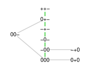
Figure 6: Potential moves over all orthants: lasso (green) and moves not minimizing $L$ (grey). We only show valid moves with $\mathbf{C}^{2}\hat{\mathbf{u}}\geq\mathbf{0}$ and $\lambda\geq 0$.

Current $\mathbf{C}$, $\lambda$	Move and candidate $\hat{\lambda}$		$i$	Comment
++-, 0	S from ++- to 0+-	$0.118$	$1$	Accepted move
	S from ++- to +0-	$0.753$	$2$	Reject, non positive $\mathbf{C}^{2}\hat{\mathbf{u}}$
	S from ++- to ++0	$0.893$	$3$	Reject, non positive $\mathbf{C}^{2}\hat{\mathbf{u}}$
0+-, 0.118	R to -+- then 0+-	$0.333$	$1$	Accepted move
	R to -+- then -0-	$1.419$	$2$	Reject, valid move but not minimum for $\hat{\lambda}$
	R to -+- then -+0	$2.128$	$3$	Reject, non positive $\mathbf{C}^{2}\hat{\mathbf{u}}$
	R to ++- then 0+-	$0.118$	$1$	Reject, $\hat{\lambda}\leq\lambda$ (this was an earlier step)
	R to ++- then +0-	$0.753$	$2$	Reject, non positive $\mathbf{C}^{2}\hat{\mathbf{u}}$
	R to ++- then ++0	$0.893$	$3$	Reject, non positive $\mathbf{C}^{2}\hat{\mathbf{u}}$
	S from 0+- to 00-	$2.426$	$2$	Reject, valid move but not minimum $\hat{\lambda}$
	S from 0+- to 0+0	$7.666$	$3$	Reject, non positive $\mathbf{C}^{2}\hat{\mathbf{u}}$
0+-, 0.333	R to -+- then 0+-	$0.333$	$1$	Reject, $\lambda\leq\lambda_{c}$ (this was an earlier step)
	R to -+- then -0-	$1.419$	$2$	Accepted move
	R to -+- then -+0	$2.128$	$3$	Reject, non positive $\mathbf{C}^{2}\hat{\mathbf{u}}$
	R to ++- then 0+-	$0.118$	$1$	Reject, $\hat{\lambda}\leq\lambda$ (this was an earlier step)
	R to ++- then +0-	$0.753$	$2$	Reject, non positive $\mathbf{C}^{2}\hat{\mathbf{u}}$
	R to ++- then ++0	$0.893$	$3$	Reject, non positive $\mathbf{C}^{2}\hat{\mathbf{u}}$
	S from 0+- to 00-	$2.426$	$2$	Reject, valid move but not minimum for $\hat{\lambda}$
	S from 0+- to 0+0	$7.666$	$3$	Reject, non positive $\mathbf{C}^{2}\hat{\mathbf{u}}$
-0-, 1.419	R to --- then 0--	$-0.571$	$1$	Reject, non positive $\mathbf{C}^{2}\hat{\mathbf{u}}$
	R to --- then -0-	$-2.179$	$2$	Reject, $\hat{\lambda}\leq\lambda$
	R to --- then --0	$-5.929$	$3$	Reject, $\hat{\lambda}\leq\lambda$
	R to -+- then 0+-	$0.333$	$1$	Reject, $\hat{\lambda}\leq\lambda$ (this was an earlier step)
	R to -+- then -0-	$1.419$	$2$	Reject, $\hat{\lambda}\leq\lambda$ (this was an earlier step)
	R to -+- then -+0	$2.128$	$3$	Reject, non positive $\mathbf{C}^{2}\hat{\mathbf{u}}$
	S from -0- to 00-	$-25.000$	$1$	Reject, $\hat{\lambda}\leq\lambda$
	S from -0- to -00	$5.429$	$3$	Accepted move
-00, 5.429	R to --0 then 0-0	$11.000$	$1$	Reject, non positive $\mathbf{C}^{2}\hat{\mathbf{u}}$
	R to --0 then -00	$-0.286$	$2$	Reject, $\hat{\lambda}\leq\lambda$
	R to -+0 then 0+0	$18.333$	$1$	Reject, non positive $\mathbf{C}^{2}\hat{\mathbf{u}}$
	R to -+0 then -00	$0.316$	$2$	Reject, $\hat{\lambda}\leq\lambda$
	R to -0- then 00-	$-25.000$	$1$	Reject, $\hat{\lambda}\leq\lambda$
	R to -0- then -00	$5.429$	$3$	Reject, $\hat{\lambda}\leq\lambda$ (this was an earlier step)
	R to -0+ then 00+	$1.000$	$1$	Reject, non positive $\mathbf{C}^{2}\hat{\mathbf{u}}$
	R to -0+ then -00	$-1.151$	$3$	Reject, $\hat{\lambda}\leq\lambda$
	S from -00 to 000	$14.000$	$1$	Accepted move, end of path

Table 3: Lasso computations for the example of Section 3.4.

Appendix 4 - Lasso R code and example

Four functions are used: lassoq is Algorithm 2; shrink is Algorithm 1, with the crucial step 1 that implements Equation (10) in the line SMCXTY/SM1; pseudo does $\mathbf{S}^{-}$ of Theorem 2 and Lhat evaluates $\hat{L}_{\mathbf{C}}$ of Equation (9).

The code is provided without guarantee. We do not accept responsibility for the accuracy of results nor for use or misuse of the code or results from it.

## Pseudoinverse of S=CX^TXC, with C a diagonal of {+-1,0} entries
pseudo<-function(XM,CM){  ## Define S, result SM, nonzero indices and invertible part of S
  S<-CM%*%t(XM)%*%XM%*%CM; Sm<-S*0;  nonzero<-diag(CM%*%CM)==1;  LM<-S[nonzero,nonzero];
  if(sum(nonzero)==0) LM<-0*LM else LM<-solve(LM)  ## Inverse
  Sm[nonzero,nonzero]<-LM; return(Sm) ## Substitute inverse in result SM and return
}

## Evaluation of the criterion L at C,\lambda
Lhat<-function(XM,YM,CM,lambda, SM=pseudo(XM,CM), CXTY=CM%*%t(XM)%*%YM)
     -sum(SM)/2*lambda^2+ sum(SM%*%CXTY)*lambda+sum(YM^2)/2-t(CXTY)%*%SM%*%CXTY/2

## Compute all possible candidate shrinkage moves at orthant CM and \lambda = Lm
shrink<-function(XM,YM,CM,Lm,TOL=10){  ## Variables for results, S^-, S^-CXTY, S^- 1
  ucc<-lambdacc<-result<-c(); SM<-pseudo(X=XM,C=CM);  SMCXTY<-SM%*%CM%*%t(XM)%*%YM;
  SM1<-apply(X=SM,MARGIN = 1,FUN=sum )
  lambdacc<-round(SMCXTY/SM1,TOL); ## << Equation (9) to compute candidate lambda >>
  for(lj in lambdacc) ucc<-cbind(ucc, round(SMCXTY-lj*SM1,TOL) )  ## The candidate \hat{u} solutions
  ### Filter results:  clear NA, Inf, \beta<0, <=\lambda  ;   apply filter and adapt size
  filtroc<-(!is.na(lambdacc)) &  (!is.infinite(lambdacc)) & (apply(ucc>=0,2,prod)==1) & (lambdacc>Lm);
  lambdacc<-lambdacc[filtroc];  ucc<-ucc[,filtroc];  if(length(ucc)==ncol(XM)) ucc<-matrix(ncol=1,ucc)
  if(length(lambdacc)>=1) ## For valid lambda, compute \beta,L from every column \hat{u}
    for(ik in 1:ncol(ucc))
      result<-rbind(result, c(lambdacc[ik], CM%*%matrix(ncol=1,ucc[,ik]),
                              Lhat(XM=XM,YM=YM,CM=CM,lambda=lambdacc[ik])  )   ) ## {lambda,beta,L}
  return(result)
}

## Lasso by orthants
lassoq<-function(XM,YM, TOL=10){  ## Initialization, beta_ols, matrix C
  res<-c(); Lm<-0; p<-ncol(XM); Beta0<-lm(YM~XM-1); ## lambda, number of variables, Beta_ols
  Cm<-diag(sign(round(Beta0$coefficients,TOL))); Cm[is.na(diag(Cm)),is.na(diag(Cm))]<-0
  res<-c(Lm,Beta0$coefficients,sum(Beta0$residuals^2)/2)  ##  initial step (lambda=0, beta, L)
  while(!identical(diag(Cm),rep(0,p))){    ###################### main loop
    ## candidates to shrink, reactivate, temporary results
    jc<-(1:p)[diag(Cm%*%Cm)!=0]; jcc<-(1:p)[diag(Cm%*%Cm)==0]; cand<-c()
    if(length(jc)<p)  ### If there are zeroes in C, first try to reactivate
      for(kk in jcc) ## kk indexes which variable to reactivate
        for(candvalue in c(-1,1)){ ## candvalue gives -+1 signs, pdate C’ to reactivate
          Cmc<-Cm; Cmc[kk,kk]<-candvalue; cand<-rbind(cand,shrink(XM = XM,YM = YM,CM = Cmc,Lm=Lm,TOL=TOL))
          }   ## end of -+1 loop, end of reactivate
    ## then perform  shrinkage step
    Cm->Cmc;  cand<-rbind(cand,shrink(XM = XM,YM = YM,CM = Cmc,Lm=Lm,TOL=TOL))
    ## Using the reactivation/shrinkage results, select the next move
    Ind<-which.min(cand[,1]);  Lm<-cand[Ind,1] ## select smallest lambda, update Lm
    res<-rbind(res, cand[Ind,] ); CmΨ<-diag(sign(cand[Ind,1+1:p])) ## update path, orthant
  }  #################### end of main loop
  return(unname(res)); ## output is (lambda, beta, L)
}

As example of the lassoq code, we compute the path for data of Table 1(a) and reproduce Table 2(a). The code needs preloading the functions of this Appendix.

X<-c(0,0,-1,1,-1,1,0,1,0,-1,-1,0,-1,0,0,-1,-1,1,0,1,-1,-1,-1,1,4,0,3,-3)
X<-matrix(X,byrow=TRUE,ncol=4); XM<-X[,-4];   YM<-matrix(ncol=1,X[,4])
lassoq(XM=XM,YM=YM) ## Columns are lambda, betas, L; each row a breakpoint

##            [,1]       [,2]      [,3]       [,4]      [,5]
## [1,]  0.0000000  0.1142857 0.8714286 -1.1857143 0.8428571
## [2,]  0.1176471  0.0000000 0.7352941 -1.0294118 1.0743945
## [3,]  0.3333333  0.0000000 0.6666667 -1.0000000 1.4444444
## [4,]  1.4186047 -0.3720930 0.0000000 -0.3953488 2.7652785
## [5,]  5.4285714 -0.4285714 0.0000000  0.0000000 5.1632653
## [6,] 14.0000000  0.0000000 0.0000000  0.0000000 7.0000000

The function lassoqw is a simple adaptation of lassoq to perform adaptive lasso. We perform the analysis of the same data with weights $w_{i}=1/|\hat{\beta}_{i}^{OLS}|^{\gamma}$, where $\gamma$ is fixed and $\hat{\beta}_{i}^{OLS}$ is the $i$-th coefficient of the least squares fit to the data. We give results below for $\gamma=0.25,1$.

lassoqw(XM=XM,YM=YM,adaptive = TRUE,gamma=0.25)

##             [,1]       [,2]      [,3]       [,4]      [,5]
## [1,]  0.00000000  0.1142857 0.8714286 -1.1857143 0.8428571
## [2,]  0.09594963  0.0000000 0.7414637 -1.0325815 1.0352911
## [3,]  1.03873325  0.0000000 0.4342734 -0.9060934 2.4139669
## [4,]  2.07061914 -0.1135323 0.0000000 -0.6283158 3.0895394
## [5,]  3.05595699  0.0000000 0.0000000 -0.6726211 3.9085728
## [6,] 11.47856765  0.0000000 0.0000000  0.0000000 6.9904572

lassoqw(XM=XM,YM=YM,adaptive = TRUE,gamma=1)

##             [,1]      [,2]      [,3]       [,4]      [,5]
## [1,]  0.00000000 0.1142857 0.8714286 -1.1857143 0.8428571
## [2,]  0.03374469 0.0000000 0.7608727 -1.0411072 0.9141630
## [3,]  2.19961666 0.0000000 0.0000000 -0.7620751 3.7633227
## [4,] 13.04285714 0.0000000 0.0000000  0.0000000 6.8261139

Appendix 5 - Elastic net R code and example

The code has the same structure of orthant lasso: Algorithm 2 is implemented in main function elastiq. The shrinking step 1 of Algoritm 1 is the call to the numerical solution of Equation (14), with two alternatives given: bisection and secant implementations in bisect and secant. The rest of functions are pseudomu and SM to compute $\mathbf{S}(\lambda)^{-}$; C2u for $\mathbf{C}^{2}\hat{\mathbf{u}}$ of Equation (12) and Ehat to compute $\hat{E}_{\mathbf{C}}$.

This code is provided without accepting any responsibility for its accuracy, use or misuse of code or results.

## Pseudo inverse of CX^TXC + \mu C^2,  here C is diagonal of {+-1,0} entries
pseudomu<-function(XM,CM,mu){
  S<-CM%*%t(XM)%*%XM%*%CM + mu*CM%*%CM; Sm<-S*0  ## big matrix
  nonzero<- diag(CM%*%CM)==1;  LM<-S[nonzero,nonzero] ## invertible submatrix
  if(sum(nonzero)==0) LM<-LM*0 else LM<-solve(LM)
  Sm[nonzero,nonzero]<-LM; return(Sm) ## Substitute inverse in result Sm and return
}

### Call to pseudomu() to compute generalized inverse S(lambda)^-
SM<-function(XM,CM,alpha=0.5,lambda)  pseudomu(XM=XM,CM=CM,mu=lambda*(1-alpha))
## Evaluate C^2\hat{u}
C2u<-function(XM,YM,CM,alpha=0.5,lambda)
  SM(XM=XM,CM=CM,alpha=alpha,lambda = lambda)%*%(CM%*%t(XM)%*%YM - alpha*lambda)
## Evaluation of criterion \hat E_C, i.e. value of E at \hat{beta}=CC^2\hat{u}=C\hat{u}
Ehat<-function(CM,XM,YM,lambda,alpha,betahat=CM%*%C2u(XM=XM,YM=YM,CM=CM,alpha=alpha,lambda=lambda))
   sum((YM-XM%*%betahat)^2)/2+lambda*alpha*sum(t(betahat)%*%CM)+lambda*(1-alpha)*sum(betahat^2)/2

## Secant to solve Equation (12) for \lambda
secant<-function(XM,YM,CM,alpha=0.5,lambda=0,l1=1.01*lambda+0.01,lhigh=max(abs(t(XM)%*%YM))/alpha,
                 Nmax=15,TOL=6,ii=1){
  i<-1; l0<-lambda; rango<-c(0, lhigh); FLAG<-TRUE; ## counter, lambda values and exit flag
  while(FLAG){
    lnew<-l1 - C2u(XM=XM,YM=YM,CM=CM,alpha=alpha,lambda = l1)[ii] * (l1-l0) /
      ( C2u(XM=XM,YM=YM,CM=CM,alpha=alpha,lambda = l1)[ii]-C2u(XM=XM,YM=YM,CM=CM,alpha=alpha,lambda = l0)[ii]   )
    l0<-l1; l1<-lnew;  i<-i+1 ## update lambda values then exit conditions
    if(i>Nmax) FLAG<-FALSE
    if( abs(l0-l1)<10^-TOL   ) FLAG<-FALSE
    if(  (abs(lnew)>10*max(rango))|| (lnew<0)){
      FLAG<-FALSE;  l1<-100*abs(lnew)
    }
  }
  if( prod(round(C2u(XM=XM,YM=YM,CM=CM,alpha=alpha,lambda = l1),TOL)>=0 )==0) l1<--1 ## check C2u>0
  return(l1)
}

## Bisection to solve Equation (12) for \lambda
bisect<-function(XM,YM,CM,alpha=0.5,lambda=0,llow=lambda,lhigh=max(abs(t(XM)%*%YM))/alpha,
                 Nmax=55,TOL=6,ii=1){ ## initial values
  i<-1; FLAG<-TRUE ## index, exit flag
  while(FLAG){ ## try and vtry are values of lambda and the respective ii-th coordinate of C2u
    try<-c(llow,mean(c(llow,lhigh)),lhigh); vtry<-c();
    for(l in try) vtry<-c(vtry, C2u(XM=XM,YM=YM,CM=CM,alpha=alpha,lambda = l)[ii])
    vtry<-sign(vtry);   i<-i+1; ## update index, lambdas to try then exit conditions
    if( prod(vtry[1:2])==-1 ) lhigh<-try[2] else llow<-try[2]
    if( abs(llow-lhigh)<10^-TOL   ) FLAG<-FALSE
    if(i>Nmax) FLAG<-FALSE
  }
  l1<-mean(try) ## Candidate lambda
  if( prod(round(C2u(XM=XM,YM=YM,CM=CM,alpha=alpha,lambda = l1),TOL)>=0 )==0) l1<--1 ## check C2u>0
  return(l1)
}

## Elastic net by orthants
elastiq<-function(XM,YM,TOL=8,alpha=0.5){## Initialization
Beta0<-lm(YM~XM-1); Cm<-diag(sign(Beta0$coefficients)); p<-ncol(XM)
res<-matrix(nrow=1, round( c(0,Beta0$coefficients,Ehat(CM=Cm,XM=XM,YM=YM,lambda=0,alpha=alpha)) , TOL) )
while(!identical( diag(Cm),rep(x=0,times=p))){   ###### main loop
  cand<-c()
  for(i in 1:p){
    if(Cm[i,i]==0){ ## first try to reactivate
      for(k in c(-1,1)){
        Cmc<-Cm;  Cmc[i,i]<-k
        for(j in (1:p)[diag(Cmc)!=0]){  ## shrink all coordinates in new orthant
        ##secant(XM=XM,YM=YM,CM=Cmc,alpha=alpha,ii=j,TOL=TOL)->lambdac ## uncomment one method
        bisect(XM=XM,YM=YM,CM=Cmc,alpha=alpha,ii = j,llow = max(res[,1]),TOL=TOL)->lambdac ## uncomment one method
        Cmc%*%C2u(XM=XM,YM=YM,CM=Cmc,alpha=alpha,lambda = lambdac)->betatemp
        cand<-rbind(cand,c(lambdac,betatemp,Ehat(CM=Cmc,XM=XM,YM=YM,lambda=lambdac,alpha=alpha)))  ## 1 reactivate
        }
      }
    } else  { ## then perform shrinkage moves
      Cmc<-Cm;  #Cmf[i,i]<-0; #Cmc[i,i]<-0;
      ##secant(XM=XM,YM=YM,CM=Cmc,alpha=alpha,ii=i,TOL=TOL)->lambdac ## uncomment one method
      bisect(XM=XM,YM=YM,CM=Cmc,alpha=alpha,ii = i,llow = max(res[,1]),TOL=TOL)->lambdac ## uncomment one method
      Cmc%*%C2u(XM=XM,YM=YM,CM=Cmc,alpha=alpha,lambda = lambdac)->betatemp
      cand<-rbind(cand,c(lambdac,betatemp,Ehat(CM=Cmc,XM=XM,YM=YM,lambda=lambdac,alpha=alpha))) ## -1 shrink
    }
  }
  cand<-round(cand,TOL);  if(!is.matrix(cand)) cand<-matrix(nrow=1,cand)
  ## Remove $\lambda$ that repeat past steps then select smallest valid \lambda, update results and orthant
  ff<-cand[,1]>max(res[,1])+10*10^-(TOL); cand<-cand[ff,];   if(!is.matrix(cand)) cand<-matrix(nrow=1,cand)
  Ind<-which.min(cand[,1]); res<-rbind(res, cand[Ind,]);   diag(Cm)<-sign(cand[Ind,1+1:p])
} ###### end of main loop
return(unname(res))
}

The example uses elastiq with $\alpha=0.5$ for the data of Table 1(a). We use the provided R functions, and XM and YM of Appendix 4 to reproduce Table 2(b). We also give another case of elastic net for the same data and $\alpha=0.9$.

## Columns are lambda, betas, L; each row a breakpoint
elastiq(XM=XM,YM=YM,TOL=8)

##            [,1]       [,2]      [,3]       [,4]      [,5]
## [1,]  0.0000000  0.1142857 0.8714286 -1.1857143 0.8428571
## [2,]  0.1459742  0.0000000 0.7315377 -1.0262653 1.0539203
## [3,]  0.2471659  0.0000000 0.7039861 -1.0132639 1.1811668
## [4,]  2.6872073 -0.3743399 0.0000000 -0.3589718 2.8979158
## [5,] 16.9614814 -0.1937892 0.0000000  0.0000000 6.4652136
## [6,] 28.0000000  0.0000000 0.0000000  0.0000000 7.0000000

elastiq(XM=XM,YM=YM,TOL=8,alpha=0.9)

##            [,1]       [,2]      [,3]       [,4]      [,5]
## [1,]  0.0000000  0.1142857 0.8714286 -1.1857143 0.8428571
## [2,]  0.1223731  0.0000000 0.7346599 -1.0288828 1.0709295
## [3,]  0.3125817  0.0000000 0.6760267 -1.0032808 1.3801569
## [4,]  1.5631239 -0.3732292 0.0000000 -0.3900203 2.7791579
## [5,]  6.5623470 -0.3918375 0.0000000  0.0000000 5.4142556
## [6,] 15.5555555  0.0000000 0.0000000  0.0000000 7.0000000

Appendix 6 - Additional figures

--++-+++++ --++-+0+++ --++-+-+++ 0-++-+-+++ 0-++-0-+++ 0-++-0-0++ 0-++---0++ 0-++0--0++ 0-++00-0++ 0-++00-0+0 00++00-0+0 00++0000+0 00+00000+0 00+0000000 0000000000	--++-+-+++ --++-0-+++ --++---+++ 0-++---+++ +-++---+++ +-++0--+++ +-++00-+++ +-+++0-+++ +0++++-+++ +0+++0-+++ 00+++0-+++ 00++00-+++ 00++000++0 00+00000+0 0000000000
(a)	(b)

Figure 9: Orthant excursion for the scaled diabetes data set, computed with (a) the orthant method and (b) glmnet.

-+-+++-++--++------++---+----+--+-++---+----+ -+-+++-++--++------0+---+----+--+-++---+----+ -+-+++-++--++-------+---+----+--+-++---+----+ -+-+++-++-0++-------+---+----+--+-++---+----+ -+-+++-++-0++-------+---+----+--+-0+---+----+ -+-+++-++-0++-------+---+----+--+--+---+----+ -+-+++-++-0++-------+---+--0-+--+--+---+----+ -+-+++-++-0++-------+---+-00-+--+--+---+----+ -+-+++-+0-0++-------+---+-00-+--+--+---+----+ -+-+++-+0-0++-------+---+-00-+--+--+--0+----+ -+-+++-+0-0++-------+---+-00-+-0+--+--0+----+ -+-+++-+0-0++-------+---+-0+-+-0+--+--0+----+ -+-+++-+0-0++-------+---+-0+-+00+--+--0+----+ -+-+++-+0-0++-0-----+---+-0+-+00+--+--0+----+ -+-+++-+0-0++-0-----+---+-0+-+00+--+--0+---0+ -+-+++-+0-0++-0-----+---+-0+-+00+--+--++---0+ -+-+++-+0-0++00-----+---+-0+-+00+--+--++---0+ -+-+++-+0-0++00-----+---+-0+-+00+--0--++---0+ -+-+++-+0-0++00-----+---+-0+-+00+--0--+0---0+ -+-+++-+0-0++00-----+---+-0+0+00+--0--+0---0+ -+-+++-+0-0++00-----+---0-0+0+00+--0--+0---0+ -+-+++-+0-00+00-----+---0-0+0+00+--0--+0---0+ -+-+++-+0-00+00-----+---0-0+0+00+--0--00---0+ -+-+++-+0-00+00-----+---0-0+0+00+--00-00---0+ -+-+++-+0-00+00-----+-0-0-0+0+00+--00-00---0+ -+-+++-+0-00+00-----+-0-000+0+00+--00-00---0+ -+-+++-+0-00+00-----+-0-000+0+00+--00-00--00+ -+-+++-+0-00+00-----+-0--00+0+00+--00-00--00+ -+-+++-+0-00+00-----+-0--00+0+00+-000-00--00+ -+-+++-+0-00+00--0--+-0--00+0+00+-000-00--00+ -+-+++0+0-00+00--0--+-0--00+0+00+-000-00--00+ -+-+0+0+0-00+00--0--+-0--00+0+00+-000-00--00+ -+-+0+0+0-00+00--0--+-0--0000+00+-000-00--00+ -+-+0+0+0-00+00--0--+-0--0000+00+0000-00--00+ -+-+0+0+0-00+00--0--+-0--0000+00+0000-00--000 -+-+0+0+0-00000--0--+-0--0000+00+0000-00--000 -+-+0+0+0-000000-0--+-0--0000+00+0000-00--000 -+-00+0+0-000000-0--+-0--0000+00+0000-00--000 -+-00+0+0-000000-0--+-00-0000+00+0000-00--000 -+-00+0+0-000000-0--+-00-0000+00+0000-000-000 -+-00+0+0-000000-0--+-00-0000+00+00000000-000 -+000+0+0-000000-0--+-00-0000+00+00000000-000 -+000+0+0-000000-0--+-0000000+00+00000000-000 -+000+0+0-000000-0--+-0000000000+00000000-000 -+000+0+0-000000-0--0-0000000000+00000000-000 -+000+0+0-000000-0--0-0000000000+000000000000 -+000+0+0-000000-00-0-0000000000+000000000000 -+000+0+0-000000000-0-0000000000+000000000000 -+00000+0-000000000-0-0000000000+000000000000 -+00000+00000000000-0-0000000000+000000000000 -+00000000000000000-0-0000000000+000000000000 -+00000000000000000-0-00000000000000000000000 -+00000000000000000-0000000000000000000000000 -+0000000000000000000000000000000000000000000 -00000000000000000000000000000000000000000000 000000000000000000000000000000000000000000000

-+-+++-++--++------++---+----+--+-++---+----+ -+-+++-++--++------0+---+----+--+-++---+----+ -+-+++-++--++-------+---+----+--+-++---+----+ -+-+++-++-0++-------+---+----+--+-++---+----+ -+-+++-++-0++-------+---+----+--+-0+---+----+ -+-+++-++-0++-------+---+----+--+--+---+----+ -+-+++-++-0++-------+---+--0-+--+--+---+----+ -+-+++-++-0++-------+---+-00-+--+--+---+----+ -+-+++-+0-0++-------+---+-00-+--+--+--0+----+ -+-+++-+0-0++-------+---+-00-+-0+--+--0+----+ -+-+++-+0-0++-------+---+-0+-+-0+--+--0+----+ -+-+++-+0-0++-0-----+---+-0+-+00+--+--0+----+ -+-+++-+0-0++-0-----+---+-0+-+00+--+--++----+ -+-+++-+0-0++-0-----+---+-0+-+00+--+--++---0+ -+-+++-+0-0++00-----+---+-0+-+00+--+--++---0+ -+-+++-+0-0++00-----+---+-0+-+00+--0--+0---0+ -+-+++-+0-0++00-----+---+-0+0+00+--0--+0---0+ -+-+++-+0-0++00-----+---0-0+0+00+--0--+0---0+ -+-+++-+0-00+00-----+---0-0+0+00+--0--00---0+ -+-+++-+0-00+00-----+---0-0+0+00+--00-00---0+ -+-+++-+0-00+00-----+-0-000+0+00+--00-00---0+ -+-+++-+0-00+00-----+-0-000+0+00+--00-00--00+ -+-+++-+0-00+00-----+-0-000+0+00+-000-00--00+ -+-+++-+0-00+00--0--+-0--00+0+00+-000-00--00+ -+-+0+-+0-00+00--0--+-0--00+0+00+0000-00--00+ -+-+0+0+0-00+00--0--+-0--0000+00+0000-00--000 -+-00+0+0-00000--0--+-0-00000+00+0000-00--000 -+-00+0+0-00000--0--+-0000000+00+0000-000-000 -+000+0+0-000000-0--+-0000000+00+0000-000-000 -+000+0+0-000000-0--+-0000000+00+00000000-000 -+000+0+0-000000-0--0-0000000000+000000000000 -+000+0+0-00000000--0-0000000000+000000000000 -+000+0+0-000000000-0-0000000000+000000000000 -+00000+0-000000000-0-0000000000+000000000000 -+0000000-000000000-0-0000000000+000000000000 -+00000000000000000-0-00000000000000000000000 -+0000000000000000000-00000000000000000000000 -+0000000000000000000000000000000000000000000 -00000000000000000000000000000000000000000000 000000000000000000000000000000000000000000000

(a)

(b)

Figure 10: Orthant excursion for simulated data with $n=55$ observations and $p=45$ variables, computed with (a) the orthant method and (b) glmnet.

References

- [1] Robert Tibshirani. Regression shrinkage and selection via the lasso. J. Roy. Statist. Soc. Ser. B, 58(1):267–288, 1996.
- [2] Trevor Hastie, Robert Tibshirani, and Jerome Friedman. The elements of Statistical Learning. Data mining, Inference and Prediction. Springer-Verlag, New York-Berlin, 2009.
- [3] Bradley Efron, Trevor Hastie, Iain Johnstone, and Robert Tibshirani. Least angle regression. Ann. Statist., 32(2):407–499, 2004. With discussion, and a rejoinder by the authors.
- [4] Ryan J. Tibshirani and Jonathan Taylor. The solution path of the generalized lasso. Ann. Statist., 39(3):1335–1371, 2011.
- [5] M. R. Osborne, Brett Presnell, and B. A. Turlach. A new approach to variable selection in least squares problems. IMA J. Numer. Anal., 20(3):389–403, 2000.
- [6] Michael R. Osborne, Brett Presnell, and Berwin A. Turlach. On the lasso and its dual. Journal of Computational and Graphical Statistics, 9(2):319–337, 2000.
- [7] H. Noguchi, Y. Ojima, and S. Yasui. Bayesian lasso with effect heredity principle. In Knoth S. and Schmid W., editors, Frontiers in Statistical Quality Control 11, pages 355–365. Springer, 2015.
- [8] Yuan Jiang, Yunxiao He, and Heping Zhang. Variable selection with prior information for generalized linear models via the prior lasso method. Journal of the American Statistical Association, 111(513):355–376, 2016. PMID: 27217599.
- [9] Jerome Friedman, Trevor Hastie, Holger Höfling, and Robert Tibshirani. Pathwise coordinate optimization. The Annals of Applied Statistics, 1(2):302 – 332, 2007.
- [10] Jerome Friedman, Robert Tibshirani, and Trevor Hastie. Regularization paths for generalized linear models via coordinate descent. Journal of Statistical Software, 33(1):1–22, 2010.
- [11] Trevor Hastie and Brad Efron. lars: Least Angle Regression, Lasso and Forward Stagewise, 2022. R package version 1.3.
- [12] Hui Zou and Trevor Hastie. Regularization and variable selection via the elastic net. J. R. Stat. Soc. Ser. B. Stat. Methodol., 67(2):301–320, 2005.
- [13] David Kepplinger. Robust variable selection and estimation via adaptive elastic net s-estimators for linear regression. Computational Statistics & Data Analysis, page 107730, 2023.
- [14] Hugo Maruri-Aguilar and Simon Lunagomez. Lasso for hierarchical polynomial models, 2020.
- [15] Jacob Bien, Jonathan Taylor, and Robert Tibshirani. A LASSO for hierarchical interactions. Ann. Statist., 41(3):1111–1141, 2013.
- [16] Li Wang, Ji Zhu, and Hui Zou. The doubly regularized support vector machine. Statistica Sinica, 16(2):589–615, 2006.
- [17] Matthias Weber, Jonas Striaukas, Martin Schumacher, and Harald Binder. Network-constrained covariate coefficient and connection sign estimation. CORE Discussion Paper 2018/18, June 2018.
- [18] Hansheng Wang and Chenlei Leng. Unified lasso estimation by least squares approximation. Journal of the American Statistical Association, 102(479):1039–1048, 2007.
- [19] Robert Tibshirani, Michael Saunders, Saharon Rosset, Ji Zhu, and Keith Knight. Sparsity and smoothness via the fused lasso. Journal of the Royal Statistical Society. Series B (Statistical Methodology), 67(1):91–108, 2005.