A New Computationally Simple Approach for Implementing Neural Networks with Output Hard Constraints

Abstract

A new computationally simple method of imposing hard convex constraints on the neural network output values is proposed. The key idea behind the method is to map a vector of hidden parameters of the network to a point that is guaranteed to be inside the feasible set defined by a set of constraints. The mapping is implemented by the additional neural network layer with constraints for output. The proposed method is simply extended to the case when constraints are imposed not only on the output vectors, but also on joint constraints depending on inputs. The projection approach to imposing constraints on outputs can simply be implemented in the framework of the proposed method. It is shown how to incorporate different types of constraints into the proposed method, including linear and quadratic constraints, equality constraints, and dynamic constraints, constraints in the form of boundaries. An important feature of the method is its computational simplicity. Complexities of the forward pass of the proposed neural network layer by linear and quadratic constraints are $O(nm)$ and $O(n^{2}m)$, respectively, where $n$ is the number of variables, $m$ is the number of constraints. Numerical experiments illustrate the method by solving optimization and classification problems. The code implementing the method is publicly available.

Keywords: neural network, hard constraints, convex set, projection model, optimization problem, classification

1 Introduction

Neural networks can be regarded as an important and effective tool for solving various machine learning tasks. A lot of tasks require to constrain the output of a neural network, i.e. to ensure the output of the neural network satisfies specified constraints. Examples of tasks, which restrict the network output, are neural optimization solvers with constraints, models generating images or parts of images in a predefined region, neural networks solving the control tasks with control actions in a certain interval, etc.

The most common approach to restrict the network output space is to add some extra penalty terms to the loss function to penalize constraint violations. This approach leads to the so-called soft constraints or soft boundaries. It does not guarantee that the constraints will be satisfied in practice when a new example feeds into the neural network. This is because the output falling outside the constraints is only penalized, but not eliminated [1]. Another approach is to modify the neural network such that it strongly predicts within the constrained output space. In this case, the constraints are hard in the sense that they are satisfied for any input example during training and inference [2].

Although many applications require the hard constraints, there are not many models that actually realize them. Moreover, most available models are based on applying the soft constraints due to their simple implementation by means of penalty terms in loss functions. In particular, Lee et al. [3] present a method for neural networks that enforces deterministic constraints on outputs, which actually cannot be viewed as hard constraints because they are substituted into the loss function.

An approach to solving problems with conical constraints of the form $Ax\leq 0$ is proposed in [2]. The model generates points in a feasible set using a predefined set of rays. A serious limitation of this method is the need to search for the corresponding rays. If to apply this approach not only to conical constraints, then we need to look for all vertices of the set. However, the number of vertices may be extremely large. Moreover, authors of [2] claim that the most general setting does not allow for efficient incorporation of domain constraints.

A general framework for solving constrained optimization problems called DC3 is described in [4]. It aims to incorporate (potentially non-convex) equality and inequality constraints into the deep learning-based optimization algorithms. The DC3 method is specifically designed for optimization problems with hard constraints. Its performance heavily relies on the training process and the chosen model architecture.

A scalable neural network architecture which constrains the output space is proposed in [5]. It is called ConstraintNet and applies an input-dependent parametrization of the constrained output space in the final layer. Two limitations of the method can be pointed out. First, constraints in ConstraintNet are linear. Second, the approach also uses all vertices of the constrained output space, whose number may be large.

A differentiable block for solving quadratic optimization problems with linear constraints, as an element of a neural network, was proposed in [6]. For a given optimization problem with a convex loss function and a set of linear constraints, the optimization layer allows finding a solution during the forward pass, and finding derivatives with respect to parameters of the loss function and constraints during the backpropagation. A similar approach, which embeds an optimization layer into a neural network avoiding the need to differentiate through optimization steps, is proposed in [7]. In contrast to [6], the method called the Discipline Convex Programming is extended to the case of arbitrary convex loss function including its parameters. According to the Discipline Convex Programming [7], a projection operator can be implemented by using a differentiable optimization layer that guarantees that the output of the neural network satisfies constraints. However, the above approaches require solving convex optimization problems for each forward pass.

Another method for solving optimization problem with linear constraints is represented in [8]. It should be noted that the method may require significant computational resources and time to solve complex optimization problems. Moreover, it solves the optimization problems only with linear constraints.

Several approaches for solving the constrained optimization problems have been proposed in [9, 10, 11, 12, 13, 14]. An analysis of the approaches can be found in the survey papers [15, 16].

To the best of our knowledge, at the moment, no approach is known that allows building layers of neural networks, the output of which satisfies linear and quadratic constraints, without solving the optimization problem during the forward pass of the neural network. Therefore, we present a new computationally simple method of the neural approximation which imposes hard linear and quadratic constraints on the neural network output values. The key idea behind the method is to map a vector of hidden parameters to a point that is guaranteed to be inside the feasible set defined by a set of constraints. The mapping is implemented by the additional neural network layer with constraints for output. The proposed method is simply extended to the case when constraints are imposed not only on the output vectors, but also on joint constraints depending on inputs. Another peculiarity of the method is that the projection approach to imposing constraints on outputs can simply be implemented in the framework of the proposed method.

An important feature of the proposed method is its computational simplicity. For example, the computational complexity of the forward pass of the neural network layer implementing the method in the case of linear constraints is $O(nm)$ and in the case of quadratic constraints is $O(n^{2}m)$, where $n$ is the number of variables, $m$ is the number of constraints.

The proposed method can be applied to various applications. First of all, it can be applied to solving optimization problems with arbitrary differentiable loss functions and with linear and quadratic constraints. The method can be applied to implement generative models with constraints. It can be used when constraints are imposed on a predefined points or a subsets of points. There are many other applications where the input and output of neural networks are constrained. The proposed method allows solving the corresponding problems incorporating the inputs as well as outputs imposed by the constraints.

Our contributions can be summarized as follows:

1. A new computationally simple method of the neural approximation which imposes hard linear and quadratic constraints on the neural network output values is proposed.

2. The implementation of the method by different types of constraints, including linear and quadratic constraints, equality constraints, constraints imposed on inputs and outputs are considered.

3. Different modifications of the proposed method are studied, including the model for obtaining solutions at boundaries of a feasible set and the projection models.

4. Numerical experiments illustrating the proposed method are provided. In particular, the method is illustrated by considering various optimization problems and a classification problem.

The corresponding code implementing the proposed method is publicly available at:

https://github.com/andruekonst/ConstraiNet/.

The paper is organized as follows. The problem of constructing a neural network imposing hard constraints on the network output value is stated in Section 2. The proposed method solving the stated problem and its modifications is considered in Section 3. Numerical experiments are given in Section 4. Conclusion can be found in Section 5.

2 The problem statement

Formally, let $z\in\mathbb{R}^{d}$ denote the input data for a neural network, and $x\in\mathbb{R}^{n}$ denote the output (prediction) of the network. The neural network can be regarded as a function $f_{\theta}:\mathbb{R}^{d}\rightarrow\mathbb{R}^{n}$ such that $x=f_{\theta}(z)$, where $\theta\in\Theta$ is a vector of trainable parameters.

Let we have a convex feasible set $\Omega\subset\mathbb{R}^{n}$ as the intersection of a set of constraints in the form of $m$ inequalities:

$$\Omega=\left\{x~{}|~{}h_{i}(x)\leq 0,~{}i=1,...,m\right\},$$ (1)

where each constraint $h_{i}(x)\leq 0$ is convex, i.e. $\forall x^{(1)},x^{(2)}:h(x^{(1)}),h(x^{(2)})\leq 0$, there holds

$$\forall\alpha\in[0,1]~{}(h(\alpha x^{(1)}+(1-\alpha)x^{(1)})\leq 0).$$ (2)

We aim to construct a neural network with constraints for outputs. In other words, we aim to construct a model $x=f_{\theta}(z):\mathbb{R}^{d}\rightarrow\Omega$ and to impose hard constraints on $x$ such that $x\in\Omega$ for all $z\in\mathbb{R}^{d}$, i.e.

$$\forall z\in\mathbb{R}^{d}~{}(f_{\theta}(z)\in\Omega).$$ (3)

3 The proposed method

To construct the neural network with constrained output vector, two fundamentally different strategies can be applied:

1. The first strategy is to project into the feasible set $\Omega$. The strategy is to build a projective differentiable layer $P(y):\mathbb{R}^{n}\rightarrow\mathbb{R}^{n}$ such that $\forall y\in\mathbb{R}^{n}~{}(P(y)\in\Omega)$. A difficulty of the approach can arise with optimizing projected points when they are outside the set $\Omega$. In this case, the projections will lie on the boundary of the feasible set, but not inside it. This case may complicate the optimization of the projected points.

2. The second strategy is to map the vector of hidden parameters to a point that is guaranteed to be inside the feasible set $\Omega$. The mapping $G(\lambda):\mathbb{R}^{k}\rightarrow\mathbb{R}^{n}$ is constructed such that $\forall\lambda\in\mathbb{R}^{k}~{}(G(\lambda)\in\Omega)$, where $\lambda$ is the vector of hidden parameters having the dimensionality $k$. This strategy does not have the disadvantages of the first strategy.

In spite of the difference between the above strategies, it turns out that the first strategy can simply be implemented by using the second strategy. Therefore, we start with a description of the second strategy.

3.1 The neural network layer with constraints for output

Let a fixed point $p$ be given inside a convex set $\Omega$, i.e. $p\in\Omega$. Then an arbitrary point $x$ from the set $\Omega$ can be represented as:

$$x=p+\alpha\cdot r,$$ (4)

where $\alpha\geq 0$ is a scale factor; $r\in\mathbb{R}^{n}$ is a vector (a ray from the point $p$).

On the other hand, for any $p,r$, there is an upper bound $\overline{\alpha}_{p,r}$ for the parameter $\alpha$, which is defined as

$$\overline{\alpha}_{p,r}=\max\left\{\alpha\geq 0~{}|~{}p+\alpha\cdot r\in\Omega\right\}.$$ (5)

At that, the segment $\left[p;~{}p+\overline{\alpha}_{p,r}\cdot r\right]$ belongs to the set $\Omega$ because $\Omega$ is convex. The meaning of the upper bound $\overline{\alpha}_{p,r}$ is to determine the point of intersection of the ray $r$ and one of the constraints.

Let us construct a layer of the neural network which maps the ray $r$ and the scale factor $\alpha_{p,r}$ as follows:

$$g_{p}(r,s)=p+\alpha_{p,r}(s)\cdot r,$$ (6)

where $\alpha_{p,r}(s)$ is a function of the layer parameter $s$ and $\overline{\alpha}_{p,r}$, which is of the form:

$$\alpha_{p,r}(s)=\sigma(s)\cdot\overline{\alpha}_{p,r},$$ (7)

$\sigma(s):\mathbb{R}\rightarrow[0,1]$ is the sigmoid function, that is, a smooth monotonic function.

Such a layer is guaranteed to fulfill the constraint

$$\forall r\in\mathbb{R}^{n},\ s\in\mathbb{R}~{}(g_{p}(r,s)\in\Omega).$$ (8)

This neural network is guaranteed to fulfil the constraints:

$$\forall z\in\mathbb{R}^{d}~{}(f_{\theta}(z)\in\Omega),$$ (9)

because the segment $[p,p+\overline{\alpha}_{p,r}\cdot r]$ belongs to $\Omega$.

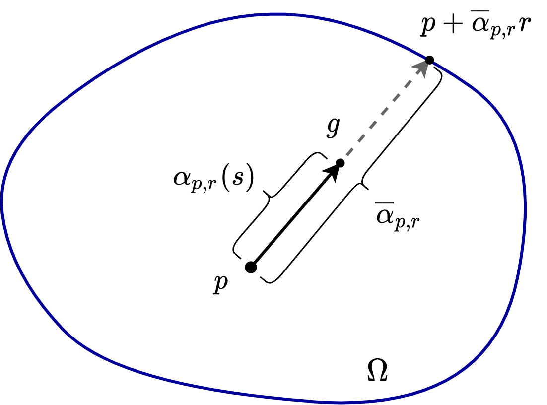
Figure 1: A scheme of the map $g_{p}(r,s)$

A scheme for mapping the ray $r$ and the scalar factor $s$ to a point inside the set $\Omega$ is shown in Fig.1. We are searching for the intersection of the ray $r$, leaving the point $p$, with the boundary of the set $p+\overline{\alpha}_{p,r}\cdot r$, and then the result of scaling is the point $g$.

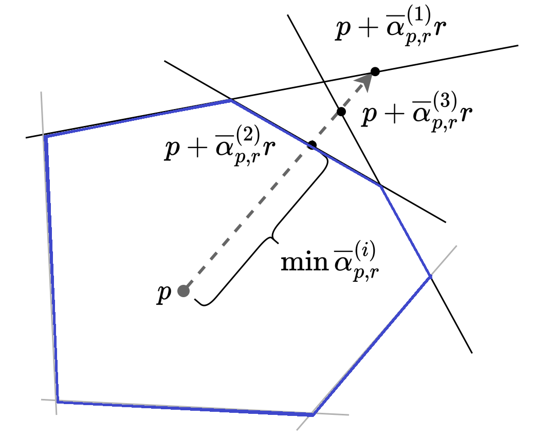
Figure 2: A scheme of searching for the upper bound $\overline{\alpha}$

For the entire systems of constraints, it is sufficient to find the upper bound $\overline{\alpha}_{p,r}$ that satisfies each of the constraints. Let $\overline{\alpha}_{p,r}^{(i)}$ be the upper bound for the parameter $\alpha$ corresponding to the $i$-th constraint $(h_{i}(x)\leq 0)$ of the system (1). Then the upper bound for the entire system of constraints is determined to satisfy the condition $[p,p+\overline{\alpha}_{p,r}\cdot r]\subseteq[p,p+\overline{\alpha}_{p,r}^{(i)}\cdot r]$, i.e. there holds

$$\overline{\alpha}_{p,r}=\min\{\overline{\alpha}_{p,r}^{(i)}\}_{i=1}^{m}.$$ (10)

A scheme of searching for the upper bound $\overline{\alpha}_{p,r}$, when linear constraints are used, is depicted in Fig.2.

Thus, the computational complexity of the forward pass of the described neural network layer is directly proportional to the number of constraints and of the computational complexity of intersection procedure with one constraint.

Theorem 1

An arbitrary vector $x\in\Omega$ can be represented by means of the layer $g_{p}(r,s)$. The output of the layer $g_{p}(r,s)$ belongs to the set $\Omega$ for its arbitrary input $(r,s)$.

Proof.

1. An arbitrary output vector $g_{p}(r,s)$ satisfies constraints that is $\forall r\in\mathbb{R}^{n},s\in\mathbb{R}$ there holds $g_{p}(r,s)\in\Omega$ because $\alpha_{p,r}(s)\leq\overline{\alpha}_{p,r}^{(i)}$, and an arbitrary segment $[p,p+\overline{\alpha}_{p,r}^{(i)}\cdot r]\subset\Omega$. Consequently, there holds $g_{p}(r,s)\in[p,p+\alpha_{p,r}(s)]\subset\Omega$.

2. An arbitrary point $x\in\Omega$ can be represented by using the layer $g_{p}(r,s)$. Indeed, let $r=x-p$, $s\rightarrow+\infty$. Then we can write $x=g_{p}(x-p,+\infty)=p+1\cdot(x-p)=x$, as was to be proved.

 

Corollary 1

For rays from the unit sphere $||r||_{2}=1$, an arbitrary point $x\in\Omega$,$\ x\neq p$ can be uniquely represented by using $g_{p}(r,s)$.

In order to obtain the model $f_{\theta}(z):\mathbb{R}^{d}\rightarrow\Omega$, outputs $r_{\theta}(z)$ and $s_{\theta}(z)$ of the neural network layers should be fed as the input to the layer $g_{p}(r,s)$:

$$f_{\theta}(z)=g(r_{\theta}(z),s_{\theta}(z)).$$ (11)

Such a combined model also forms a neural network that can be trained by the error backpropagation algorithm.

Corollary 2

The output of the neural network $f_{\theta}(z)$ always satisfies the constraints which define the set $\Omega$.

3.2 Linear constraints

In the case of linear constraints $\overline{\alpha}(p,r)$, the upper bound is determined by the intersection of the ray from point $p$ to direction $r$ with the set of constraints.

Let us consider the intersection with one linear constraint of the form:

$$a_{i}^{T}x\leq b_{i}.$$ (12)

Then the upper bound for the parameter $\alpha$ is determined by solving the following system of equations:

$$\begin{cases}x=p+\alpha\cdot r,\\ a_{i}^{T}x=b_{i},\\ \alpha\geq 0.\end{cases}$$ (13)

This implies that there holds when a solution exists:

$$a_{i}^{T}p+\alpha\cdot a_{i}^{T}r=b_{i},$$ (14)

$$\overline{\alpha}_{p,r}^{(i)}=\frac{b_{i}-a_{i}^{T}p}{a_{i}^{T}r}.$$ (15)

If $a_{i}^{T}r=0$ or $\overline{\alpha}_{i}(p,r)<0$, then the system (13) does not have any solution. In this case, $\overline{\alpha}_{i}$ can be taken as $+\infty$.

Let we have the system

$$\begin{cases}a_{1}^{T}x\leq b_{1},\\ \dots\\ a_{N}^{T}x\leq b_{m},\end{cases}$$ (16)

and for each inequality, the upper bound $\overline{\alpha}_{p,r}^{(i)}$ is available. Then the upper bound for the whole system of inequalities (16) is determined as:

$$\overline{\alpha}_{p,r}=\min\left\{\overline{\alpha}_{p,r}^{(i)}\right\}_{i=1}^{m}.$$ (17)

In the case of linear constraints, the computational complexity of the forward pass of the neural network layer is $O(nm)$.

3.3 Quadratic constraints

Let the $i$-th quadratic constraint be given in the form:

$$\frac{1}{2}x^{T}P^{(i)}x+q_{i}^{T}x\leq b_{i},$$ (18)

where the matrix $P^{(i)}$ is positive semidefinite. Then the intersection of the ray with the constraint is given by the equation:

$$\frac{1}{2}(p+\alpha\cdot r)^{T}P^{(i)}(p+\alpha\cdot r)+q_{i}^{T}(p+\alpha\cdot r)=b_{i}.$$ (19)

It is equivalent to the equation:

$$(r^{T}P^{(i)}r)\alpha^{2}+2(p^{T}P^{(i)}r+q_{i}^{T}r)\alpha+(2q_{i}^{T}p+p^{T}P^{(i)}p-2b_{i})=0.$$ (20)

Depending on the coefficient at $\alpha^{2}$, two cases can be considered:

1. If $r^{T}P^{(i)}r=0$, then the equation is linear and has the following solution:

   $$\alpha=-\frac{q_{i}^{T}p+\frac{1}{2}p^{T}P^{(i)}p-b_{i}}{p^{T}P^{(i)}r+q_{i}^{T}r}.$$ (21)

2. If $r^{T}P^{(i)}r>0$, then there exist two solutions. However, we can select only the larger positive solution corresponding to the movement in the direction of the ray. This solution is:

   $$\alpha=-\frac{-(p^{T}P^{(i)}r+q_{i}^{T}r)+\sqrt{D/4}}{r^{T}P^{(i)}r},$$ (22)

   $$\frac{D}{4}=(p^{T}P^{(i)}r+q_{i}^{T}r)^{2}-(r^{T}P^{(i)}r)\cdot(2q_{i}^{T}p+p^{T}P^{(i)}p-2b_{i}),$$ (23)

   because the denominator is positive.

It should be noted that the case $r^{T}P^{(i)}r<0$ is not possible because the matrix is positive semidefinite. Otherwise, the constraint would define a non-convex set.

If $\alpha\geq 0$, then the upper bound is $\overline{\alpha}_{p,r}^{(i)}=\alpha$. Otherwise, if the ray does not intersects the constraint, then there holds $\overline{\alpha}_{p,r}^{(i)}=+\infty$.

Similarly to the case of linear constraints, if a system of the following quadratic constraints is given:

$$\begin{cases}\frac{1}{2}x^{T}P^{(1)}x+q_{1}^{T}x\leq b_{1},\\ \dots\\ \frac{1}{2}x^{T}P^{(m)}x+q_{N}^{T}x\leq b_{m},\end{cases}$$ (24)

then the upper bound for the system is

$$\overline{\alpha}_{p,r}=\min\{\overline{\alpha}_{p,r}^{(i)}\}_{i=1}^{m}.$$ (25)

In the case of quadratic constraints, the computational complexity of the forward pass of the neural network layer is $O(n^{2}m)$.

3.4 Equality constraints

Let us consider the case, when the feasible set is defined by a system of linear equalities and inequalities of the form:

$$x\in\Omega\iff\begin{cases}Ax\leq b,\\ Qx=p,\end{cases}$$ (26)

In this case, the problem can be reduced to (1) that is it can be reduced to a system of inequalities. In order to implement that, we find and fix a vector $u$, satisfying the system $Qu=p$. If the system does not have solutions, then the set $\Omega$ is empty. If there exists only one solution, then the set $\Omega$ consists of one point. Otherwise, there exist an infinite number of solutions, and it is sufficiently to choose any of them, for example, by solving the least squares problem:

$$||Qu-p||^{2}\rightarrow\min.$$ (27)

Then we find a matrix $R$ which is the kernel basis matrix $Q$, that is $R$ satisfies the following condition:

$$\forall w~{}\left(QRw=0\right).$$ (28)

The matrix $R$ can be obtained by using the SVD decomposition of $Q\in\mathbb{R}^{\mu\times n}$ as follows:

$$USV=Q,$$ (29)

where $U\in\mathbb{R}^{\mu\times\mu}$ is the complex unitary matrix, $S\in\mathbb{R}^{\mu\times n}$ is the rectangular diagonal matrix with non-negative real numbers on the diagonal, $V\in\mathbb{R}^{n\times n}$ is the conjugate transpose of the complex unitary matrix (the right singular vectors), it contains ordered non-zero diagonal elements.

Then the matrix $R$ is defined as

$$R=\left(v_{1},\dots,v_{\delta}\right),$$ (30)

where $\delta$ is the number of zero diagonal elements of $S$, $v_{1},\dots,v_{\delta}$ are columns of the matrix $V$.

Hence, there holds

$$\forall w\in\mathbb{R}^{\delta}~{}\left(Q(Rw+u)=p\right).$$ (31)

A new system of constraints imposed on the vector $w$ is defined as:

$$A(Rw+u)\leq b,$$ (32)

or in the canonical form:

$$Bw\leq t,$$ (33)

where $B=AR$, $t=b-Au$.

So, $w$ is the vector of variables for the new system of inequalities (33). For any vector $w$, the vector $x$ satisfying the initial system (26) can be reconstructed as $x=Rw+u$.

In sum, the resulting model will be defined as

$$f_{\theta}(z)=R\widetilde{f}_{\theta}(z)+u,$$ (34)

where $\widetilde{f}_{\theta}(z)$ is the model for constraints (33).

Let us consider a more general case when an arbitrary convex set as the intersection of the convex inequality constraints (1) is given, but an additional constraint is equality, i.e. there holds:

$$x\in\Omega\iff\begin{cases}h_{i}(x)\leq 0,\\ Qx=p.\end{cases}$$ (35)

In this case, we can also apply the variable replacement to obtain new (possibly non-linear) constraints of the form:

$$x\in\Omega\iff\begin{cases}h_{i}(Rw+u)\leq 0,\\ x=Rw+u,\end{cases}\iff\begin{cases}\tilde{h}_{i}^{(R,u)}(w)\leq 0,\\ x=Rw+u.\end{cases}$$ (36)

In sum, the model can be used for generating solutions $\widetilde{f}_{\theta}(z)$, satisfying the non-linear constraints $\tilde{h}_{i}^{(R,u)}(\widetilde{f}_{\theta}(z))$, and then solutions for $x$ are obtained through  (34).

3.5 Constraints imposed on inputs and outputs

In practice, it may be necessary to set constraints not only on the output vector $f_{\theta}(z)$, but also joint constraints depending on some inputs. Suppose, an convex set of $\mu$ constraints imposed on the input $z$ and the output $f_{\theta}(z)$ is given:

$$\Lambda\subset\mathbb{R}^{k}\times\mathbb{R}^{n},$$ (37)

that is, for any $z$, the model $f_{\theta}(z)$ has to satisfy:

$$y=\begin{bmatrix}f_{\theta}(z)\\ z\end{bmatrix}\in\Lambda.$$ (38)

Here $y$ is the concatenation of $f_{\theta}(z)$ and $z$. If the feasible set is given as an intersection of convex constraints:

$$\Lambda=\left\{y~{}|~{}\Gamma_{i}(y)\leq 0,~{}i=1,...,m\right\}.$$ (39)

Then for a fixed $z$, a new system of constraints imposed only on the output vector $f_{\theta}(z)$ can be built by means of the substitution:

$$G(z)=\left\{z~{}|~{}\gamma_{i}(x;z)\leq 0,~{}i=1,...,m\right\}$$ (40)

where $\gamma_{i}(x;z)$ is obtained by substituting $z$ into $\Gamma_{i}$.

Here $\gamma_{i}$ depends on $z$ as fixed parameters, and only $x$ is a variable. For example, if $\Gamma_{i}$ is a linear function, then, after substituting parameters, the constraint $\gamma_{i}(x;z)\leq 0$ will be a new linear constraint on $x$, or it will automatically be fulfilled. If $\Gamma_{i}$ is a quadratic function, then the constraint on $x$ is either quadratic or linear, or automatically satisfied.

New dynamic constraints imposed on the output and depending on the input $z$ are

$$f_{\theta}(z)\in G(z),$$ (41)

under condition the input $z$ is from the admissible set

$$z\in\left\{z~{}|~{}\exists x:\left[\genfrac{}{}{0.0pt}{}{x}{z}\right]\in\Lambda\right\}.$$ (42)

It can be seen from the above that the dynamic constraints can change when $z$ is changing,

3.6 Projection model

Note that using the proposed neural network layer with constraints imposed on outputs, a projection can be built as a model that maps points to the set $\Omega$ and has the idempotency property, that is:

$$\forall x\in\mathbb{R}^{n}~{}(f_{\theta}(f_{\theta}(x))=f_{\theta}(x)).$$ (43)

In other words, the model, implementing the identity substitution inside the set $\Omega$ and mapping points, which are outside the set $\Omega$, inside $\Omega$, can be represented as:

$$\begin{cases}\forall x\in\Omega~{}(f_{\theta}(x)=x),\\ \forall x\notin\Omega~{}(f_{\theta}(x)\in\Omega).\end{cases}$$ (44)

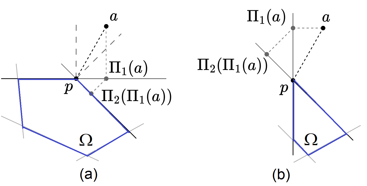
Figure 3: Difficulties of the orthogonal projection onto the intersection of convex constraints

The model can be implemented in two ways:

1. The first way is to train the model $f_{\theta}(z)=g(r_{\theta}(z),s_{\theta}(s))$ to obtain the identity substitution by means of minimizing the functional that penalizes the distance between the image and the preimage. This can construct an approximation of an arbitrary projection. For example, we can write for the orthogonal projection by using the $L_{p}$-norm the following functional:

   $$\mathcal{L}=\frac{1}{N}\sum_{i=1}^{N}\left\|f_{\theta}(x_{i})-x_{i}\right\|_{p}.$$ (45)

   As a result, the output of the model always satisfies the constraints, but the idempotency property cannot be guaranteed, since the minimization of the empirical risk does not guarantee a strict equality and even an equality with an error $\varepsilon$ on the entire set $\Omega$. Nevertheless, this approach can be used when it is necessary to build the projective models for complex metrics, for example, those defined by neural networks.

2. The central projection can be obtained without optimizing the model by means of specifying the ray $r_{\theta}(z):=z-p$. In this case, the scale factor must be specified explicitly without the sigmoid as: $\alpha_{p,r}(s)=\min\{1,\overline{\alpha}_{p,r}\}$.

   Then we can write

   $$\tilde{g}_{p}(r(x)) =p+\min\{1,\overline{\alpha}_{p,(x-p)}\}\cdot(x-p)$$

   $$=\left\{\begin{array}[c]{cc}x,&\overline{\alpha}_{p,(x-p)}\geq 1,\\ (1-\overline{\alpha}_{p,(x-p)})p+\overline{\alpha}_{p,(x-p)}x,&\text{otherwise.}\end{array}\right.$$ (48)

   It should be pointed out that other projections, for example, the orthogonal projection by using the $L_{2}$-norm, cannot be obtained in the same way. Two examples illustrating two cases of the relationship between $\Omega$ and a point $a$, which has to be projected on $\Omega$, are given in Fig.3 where the orthogonal projections of the point $a$ are denoted as $\Pi_{i}(a)$. It can be seen from Fig.3 that the point $a$ must be projected to the point $p$ located at the intersection of constraints. The projection on the nearest constraint as well as successive projections on constraints do not allow mapping the point $a$ to the nearest point inside the set $\Omega$.

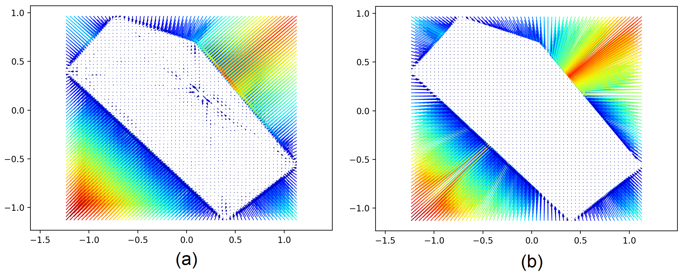
Figure 4: Illustrative examples of the projection models for linear constraints: (a) the orthogonal approximated projection, (b) the central projection

The implementation examples of the projection model are shown in Fig.4. The set $\Omega$ is formed by means of linear constraints. For each of the examples, a vector field (the quiver plot) depicted as the set of arrows is depicted where the beginning of each arrow corresponds to the preimage, and the end corresponds to its projection into the set of five constraints. On the left picture (Fig.4(a)), results of the approximate orthogonal projection implemented by a neural network consisting of five layers are shown. The network parameters were optimized by minimizing (45) with the learning rate $10^{-2}$ and the number of iterations $1000$. It can be seen from the left picture that there are artifacts in the set $\Omega$, which correspond to areas with the large approximation errors. On the right picture (Fig.4(b)), the result of the neural network without trainable parameters is depicted. The neural network implements the central projection here. It can be seen from Fig.4(b) that there are no errors when the central projection is used.

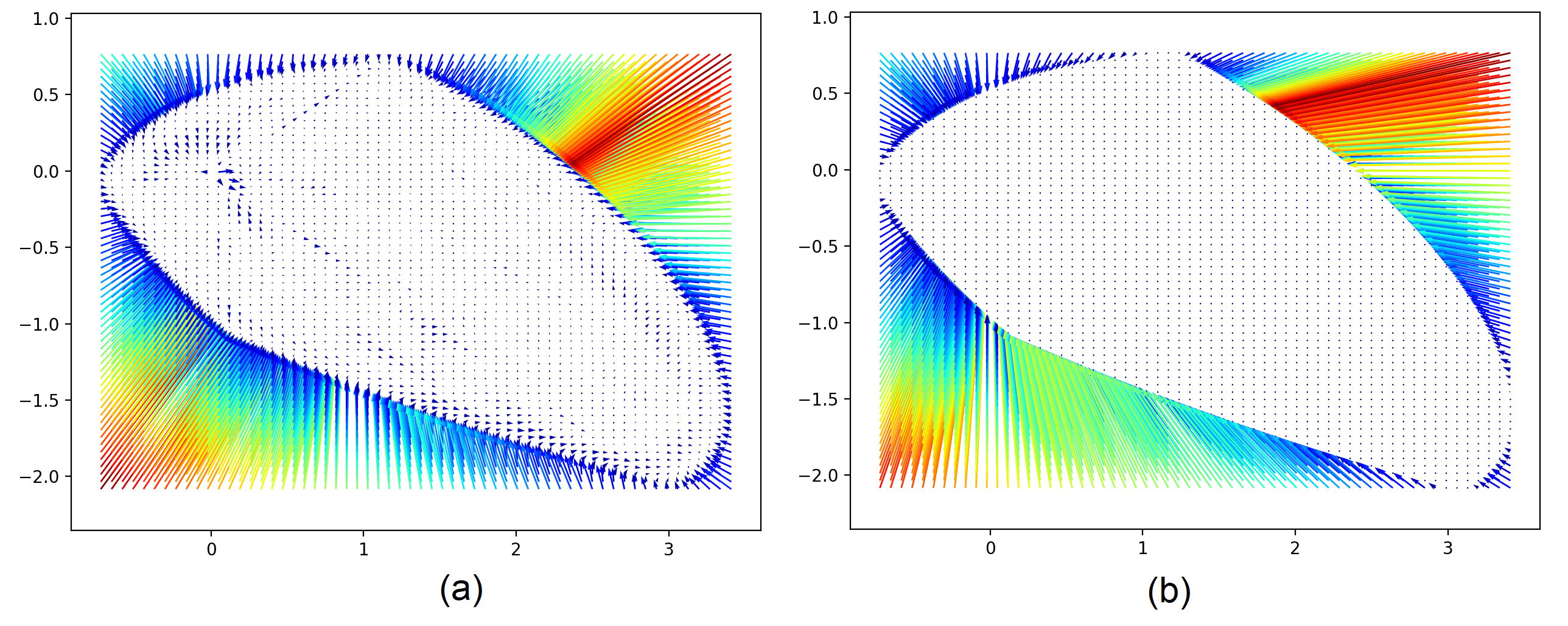
Figure 5: Examples of the projection models for quadratic constraints: (a) the orthogonal approximated projection, (b) the central projection

Similar examples for three quadratic constraints are shown in Fig.5.

3.7 Solutions at boundaries

In addition to the tasks considered above, the developed method can be applied to obtain solutions in a non-convex boundary set denoted as $\partial\Omega$. Suppose $\sigma(s)=1$. Then we can write

$$g(r)=p+\overline{\alpha}(p,r)\cdot r\in\partial\Omega.$$ (49)

The above implies that $g(r)$ is on the boundary by $r\neq\mathbf{0}$.

It is noteworthy that this approach allows us to construct a mapping onto a non-convex connected union of convex sets. On the other hand, an arbitrary method based on a convex combination of basis vectors, where weights of the basis are computed using the softmax operation, allows us to build points only inside the feasible set, but not at the boundary.

As an example, consider the problem of projecting points onto the boundary of a convex set:

$$\begin{array}[c]{c}\min\quad||z-f_{\theta}(z)||_{p}\\ \text{s.t.}\quad f_{\theta}(z)\in\partial\Omega,\end{array}$$ (50)

where $||\cdot||_{p}$ is the $p$-th norm.

Illustrative examples of projection onto an area defined by a set of linear constraints for the $L_{1}$ and $L_{2}$-norms are shown in Fig.6 where the left picture (Fig.6(a)) corresponds to the $L_{1}$-norm whereas the right picture (Fig.6(b)) considers projections for the $L_{2}$-norm. To solve each of the problems, a neural network consisting of $5$ layers of size $100$ and minimizing (50) is trained. Its set of values is given as $\partial\Omega$.

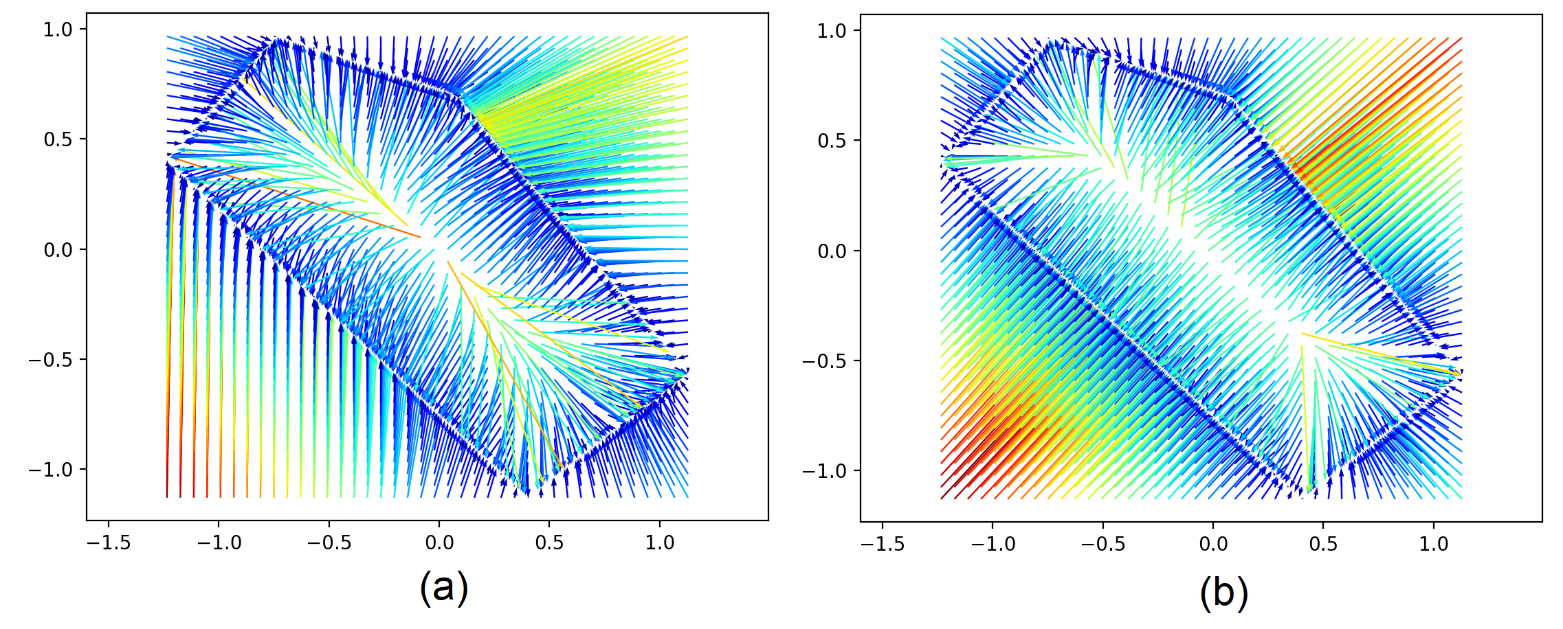
Figure 6: Illustrative examples of approximation of the projection onto the boundary by using: (a) the $L_{1}$-norm, (b) the $L_{2}$-norm

3.8 A general algorithm of the method

For systems of constraints containing linear equality constraints as well as linear and quadratic inequality constraints, the general algorithm consists of the following steps:

1. Eliminate the linear equality constraints.

2. Construct a new system of linear and quadratic constraints in the form of inequalities.

3. Search for interior point $p$.

4. Train a neural network $\tilde{f}^{(\geq)}_{\theta}(z)$ for the inequality constraints.

5. Train the final neural network $f_{\theta}(z)$, satisfying all constraints.

4 Numerical experiments

4.1 Optimization problems

A neural network with constraints imposed on outputs should at least allow finding a solution to the constrained optimization problems. To implement that for each particular optimization problem, the vector of input parameters $z_{i}$ is optimized so as to minimize the loss function $l_{i}\left(f_{\theta}(z_{i})\right)$. For testing the optimization method with constraints, $50$ sets of optimization problems (objective functions and constraints) with variables of dimensionality $2$, $5$, and $10$ are randomly generated. In each set of problems, we generate different numbers of constraints: $20$, $50$, $100$, and $200$. The linear and quadratic constraints are separately generated to construct different sets of optimization problems. The constraints are generated so that the feasible set $\Omega$ is bounded (that is, it does not contain a ray that does not cross boundaries of $\Omega$).

To generate each optimization problem, $m$ constraints are first generated, then parameters of the loss functions are generated. For systems of linear constraints, the following approach is used: a set of $m$ vectors $a_{1},\dots,a_{m}\sim\mathcal{N}(0,I)$ is generated, which simultaneously specify points belonging to hyperplanes and normals to these hyperplanes. Then the right side of the constraint system is:

$$b_{i}=a_{i}^{T}a_{i},$$ (51)

and the whole system of linear constraints:

$$\Omega=\left\{x~{}|~{}a_{i}^{T}x\leq b_{i},~{}i=1,...,m\right\}.$$ (52)

For system of quadratic constraints, positive semidefinite matrices $P^{(i)}$ and vectors $q_{i}\sim\mathcal{N}(0,I)$, $i=1,...,m$, are first generated. Then the constraints are shifted in such a way as to satisfy the constraints with some margin $b_{i}>0$. Hence, we obtain the system of quadratic constraints:

$$\Omega=\left\{x~{}|~{}x^{T}P^{(i)}x+q_{i}^{T}x\leq b_{i},~{}i=1,...,m\right\}.$$ (53)

The relative error is used for comparison of the models. It is measured by the value of the loss function of the obtained solution $l_{i}(f_{\theta}(x_{i}))$ with respect to the loss function of the reference solution $l_{i}(x_{i}^{\ast})$:

$$RE=\frac{\max\left\{0,l_{i}\left(f_{\theta}(x_{i})\right)-l_{i}(x_{i}^{\ast})\right\}}{|l_{i}(x_{i}^{\ast})|}\cdot 100\%.$$ (54)

The reference solutions are obtained using the OSQP algorithm [17] designed exclusively for solving the linear and quadratic optimization problems.

Tables 1 and 2 show relative errors for optimization problems with linear loss functions and linear and quadratic constraints, respectively, where $m$ is the number of constraints, $n$ is the number of variables in the optimization problems. The relative errors are shown in tables according to percentiles ($25\%$, $50\%$, $75\%$, $100\%$) of the probability distribution of optimization errors, which are obtained as a result of multiple experiments. Tables 3 and 4 show relative errors for optimization problems with quadratic loss functions and linear and quadratic constraints, respectively.

It can be seen from Tables 1-4 that the proposed method allows us to optimize the input parameters $r$ and $s$ for the proposed layer. One can see that the introduced layer does not degrade the gradient for the whole neural network.

Table 1: Relative errors for problems with linear loss functions and linear constraints

$m$	$n$	$25\%$	$50\%$	$75\%$	$100\%$
	$2$	$8.3\cdot 10^{-6}$	$3.6\cdot 10^{-5}$	$1.8\cdot 10^{-4}$	$1.3\cdot 10^{-2}$
$50$	$5$	$1.9\cdot 10^{-3}$	$2.4\cdot 10^{-3}$	$3.3\cdot 10^{-3}$	$3.5\cdot 10^{-2}$
	$10$	$1.1\cdot 10^{-2}$	$1.4\cdot 10^{-2}$	$2.3\cdot 10^{-2}$	$1.8\cdot 10^{-1}$
	$2$	$2.4\cdot 10^{-6}$	$2.6\cdot 10^{-5}$	$1.8\cdot 10^{-4}$	$6.7\cdot 10^{-3}$
$100$	$5$	$1.8\cdot 10^{-3}$	$2.1\cdot 10^{-3}$	$3.2\cdot 10^{-3}$	$6.4\cdot 10^{-1}$
	$10$	$9.1\cdot 10^{-3}$	$1.1\cdot 10^{-2}$	$1.3\cdot 10^{-2}$	$1.3\cdot 10^{-1}$
	$2$	$4.5\cdot 10^{-6}$	$1.5\cdot 10^{-5}$	$1.7\cdot 10^{-4}$	$7.9\cdot 10^{-2}$
$200$	$5$	$1.7\cdot 10^{-3}$	$2.6\cdot 10^{-3}$	$3.8\cdot 10^{-3}$	$1.0\cdot 10^{-2}$
	$10$	$8.4\cdot 10^{-3}$	$1.2\cdot 10^{-2}$	$1.5\cdot 10^{-2}$	$9.9\cdot 10^{-2}$

Table 2: Relative errors for problems with linear loss functions and quadratic constraints

$m$	$n$	$25\%$	$50\%$	$75\%$	$100\%$
	$2$	$5.5\cdot 10^{-6}$	$1.3\cdot 10^{-4}$	$1.6\cdot 10^{-3}$	$1.6\cdot 10^{-2}$
$50$	$5$	$3.4\cdot 10^{-6}$	$7.7\cdot 10^{-5}$	$9.9\cdot 10^{-4}$	$7.5\cdot 10^{-2}$
	$10$	$3.5\cdot 10^{-14}$	$4.3\cdot 10^{-6}$	$1.8\cdot 10^{-4}$	$3.3\cdot 10^{-3}$
	$2$	$8.0\cdot 10^{-6}$	$1.6\cdot 10^{-4}$	$1.8\cdot 10^{-3}$	$2.6\cdot 10^{-2}$
$100$	$5$	$7.3\cdot 10^{-5}$	$8.1\cdot 10^{-4}$	$3.7\cdot 10^{-3}$	$6.9\cdot 10^{-2}$
	$10$	$3.1\cdot 10^{-6}$	$1.3\cdot 10^{-5}$	$8.2\cdot 10^{-4}$	$1.7\cdot 10^{-2}$
	$2$	$1.1\cdot 10^{-5}$	$3.1\cdot 10^{-4}$	$1.5\cdot 10^{-3}$	$6.0\cdot 10^{-2}$
$200$	$5$	$1.6\cdot 10^{-4}$	$1.1\cdot 10^{-3}$	$3.8\cdot 10^{-3}$	$1.7\cdot 10^{-1}$
	$10$	$5.3\cdot 10^{-6}$	$2.8\cdot 10^{-4}$	$1.4\cdot 10^{-3}$	$1.2\cdot 10^{-2}$

Table 3: Relative errors for problems with quadratic loss functions and linear constraints

$m$	$n$	$25\%$	$50\%$	$75\%$	$100\%$
	$2$	$2.0\cdot 10^{-5}$	$3.9\cdot 10^{-5}$	$8.7\cdot 10^{-5}$	$1.5\cdot 10^{-4}$
$50$	$5$	$1.0\cdot 10^{-3}$	$1.2\cdot 10^{-3}$	$1.8\cdot 10^{-3}$	$5.5\cdot 10^{-3}$
	$10$	$5.0\cdot 10^{-3}$	$6.9\cdot 10^{-3}$	$8.9\cdot 10^{-3}$	$1.5\cdot 10^{-2}$
$100$	$2$	$1.4\cdot 10^{-5}$	$5.4\cdot 10^{-5}$	$8.5\cdot 10^{-5}$	$1.4\cdot 10^{-4}$
	$5$	$8.7\cdot 10^{-4}$	$1.6\cdot 10^{-3}$	$2.5\cdot 10^{-3}$	$4.5\cdot 10^{-3}$
	$10$	$5.6\cdot 10^{-3}$	$8.0\cdot 10^{-3}$	$1.1\cdot 10^{-2}$	$1.8\cdot 10^{-2}$
$200$	$2$	$1.5\cdot 10^{-5}$	$5.0\cdot 10^{-5}$	$1.0\cdot 10^{-4}$	$2.0\cdot 10^{-4}$
	$5$	$9.6\cdot 10^{-4}$	$1.3\cdot 10^{-3}$	$1.9\cdot 10^{-3}$	$3.9\cdot 10^{-3}$
	$10$	$6.3\cdot 10^{-3}$	$7.7\cdot 10^{-3}$	$1.1\cdot 10^{-2}$	$1.6\cdot 10^{-2}$

Table 4: Relative errors for problems with quadratic loss functions and quadratic constraints

$m$	$n$	$25\%$	$50\%$	$75\%$	$100\%$
	$2$	$5.4\cdot 10^{-6}$	$7.1\cdot 10^{-6}$	$3.6\cdot 10^{-5}$	$4.4\cdot 10^{-4}$
$50$	$5$	$2.5\cdot 10^{-4}$	$4.9\cdot 10^{-4}$	$1.1\cdot 10^{-3}$	$3.7\cdot 10^{-3}$
	$10$	$2.5\cdot 10^{-3}$	$3.5\cdot 10^{-3}$	$5.7\cdot 10^{-3}$	$1.2\cdot 10^{-2}$
	$2$	$4.4\cdot 10^{-6}$	$6.0\cdot 10^{-6}$	$3.5\cdot 10^{-5}$	$7.6\cdot 10^{-3}$
$100$	$5$	$4.4\cdot 10^{-4}$	$8.9\cdot 10^{-4}$	$1.4\cdot 10^{-3}$	$3.0\cdot 10^{-3}$
	$10$	$3.0\cdot 10^{-3}$	$4.3\cdot 10^{-3}$	$6.1\cdot 10^{-3}$	$1.5\cdot 10^{-2}$
	$2$	$5.7\cdot 10^{-6}$	$1.2\cdot 10^{-5}$	$3.9\cdot 10^{-5}$	$1.2\cdot 10^{-4}$
$200$	$5$	$3.2\cdot 10^{-4}$	$5.9\cdot 10^{-4}$	$1.2\cdot 10^{-3}$	$3.6\cdot 10^{-3}$
	$10$	$3.4\cdot 10^{-3}$	$4.9\cdot 10^{-3}$	$7.2\cdot 10^{-3}$	$1.2\cdot 10^{-2}$

An alternative way to solve the problem is to use optimization layers proposed in [6] or [7]. However, this solution is not justified due to the performance reasons. For example, consider a problem with quadratic constraints and a linear loss function from previous experiments. In this problem, parameters, which are fed to the input of the neural network, are optimized in such a way as to minimize the loss function depending on the network output. By means of the optimization layer, the problem of projection into constraints of the form (50) is solved in this case instead of solving the original optimization problem.

To compare the method [6, 7] with the proposed method, the library CVXPYLayers [7] is used, which allows us to set differentiable optimization layers within the neural network. Fig.7 compares the optimization time of the input vector by the same hyperparameters under condition that the algorithm CVXPYLayers is stopped after five minutes from the beginning of the optimization process even if the optimization is not completed. It can be seen from Fig.7 that the proposed algorithm requires significantly smaller times to obtain the solution. It should be noted that this experiment illustrates the inexpediency of constructing the constrained neural networks by solving the projection optimization problem during the forward pass. Nevertheless, the use of such layers is justified if, for example, it is required to obtain a strictly orthogonal projection.

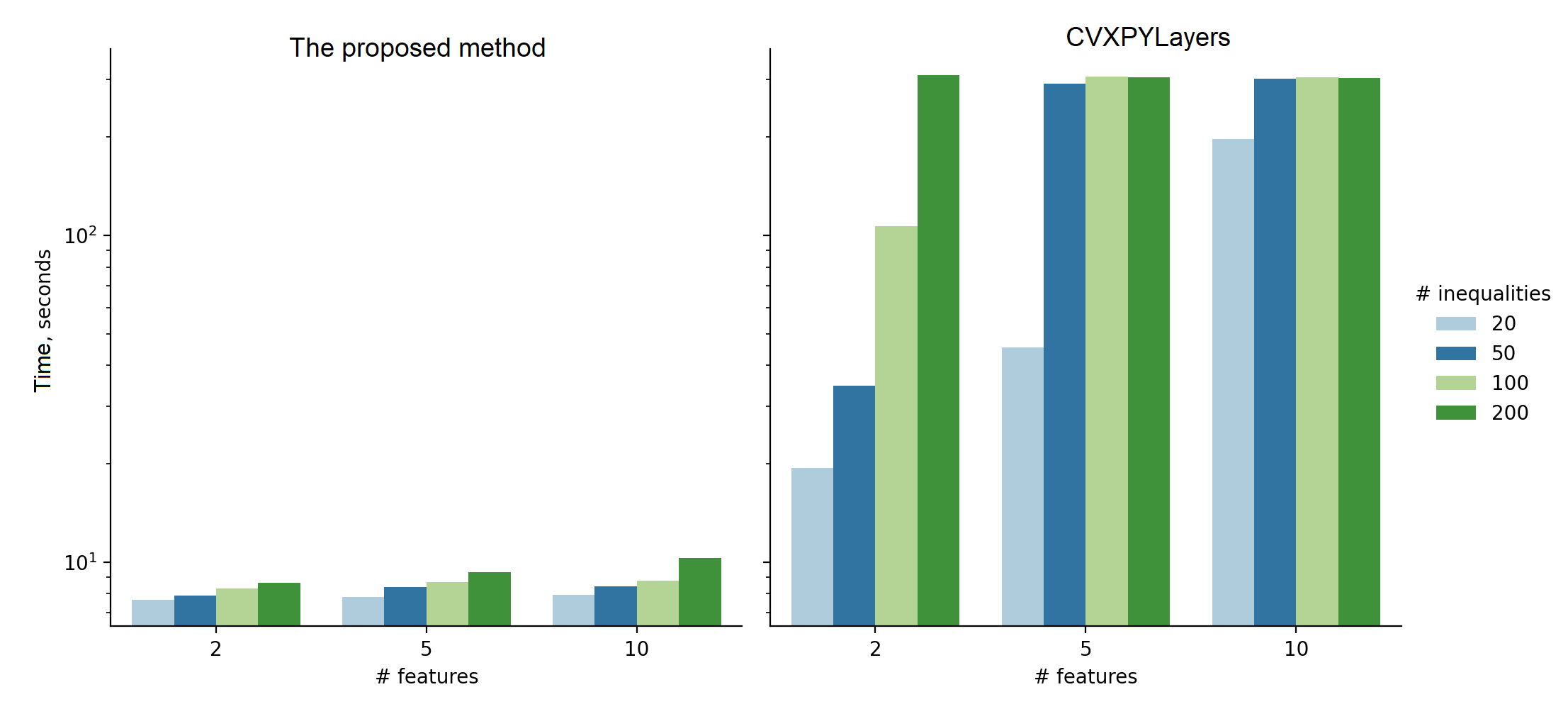
Figure 7: Comparison of the computation time of the proposed neural network and the projection using CVXPYLayers

The proposed structure of the neural network allows us to implement algorithms for solving arbitrary problems of both convex and non-convex optimization. For example, Fig.8 shows optimization trajectories for the Rosenbrock function [18] with quadratic constraints:

$$\mathcal{L}_{Ros}(x)=(1-x_{1}^{2})+100(x_{2}-x_{1}^{2})^{2},$$ (55)

$$\Omega_{Ros}=\left\{x~{}|~{}x_{1}^{2}+x_{2}^{2}\leq 2\right\}.$$ (56)

This function with constraints has a global minimum at the point $(1,1)$. The bound for the constraint set $\Omega_{Ros}$ is depicted by the large black circle. For updating the parameters, $2000$ iterations of the Adam algorithm are used with the learning rate $0.1$. $9$ points on a uniform grid from $-0.75$ to $0.75$ are chosen as starting points. For each starting point, an optimization trajectory is depicted such that its finish is indicated by a white asterisk. Three different scenarios are considered:

1. The central projection optimizes the input of a layer with the constrained output that performs the central projection. Such a layer implements the identity mapping inside the constraints and maps the outer points to the boundary.

2. The hidden space $(r,s)$ optimizes the input parameters of the proposed layer with constraints ($r$ is the ray, $s$ is the scalar that defines a shift along the ray).

3. The projection neural network is a neural network which consists of $5$ fully connected layers of size $100$ and the proposed layer with constraints. The input parameters of the entire neural network are optimized.

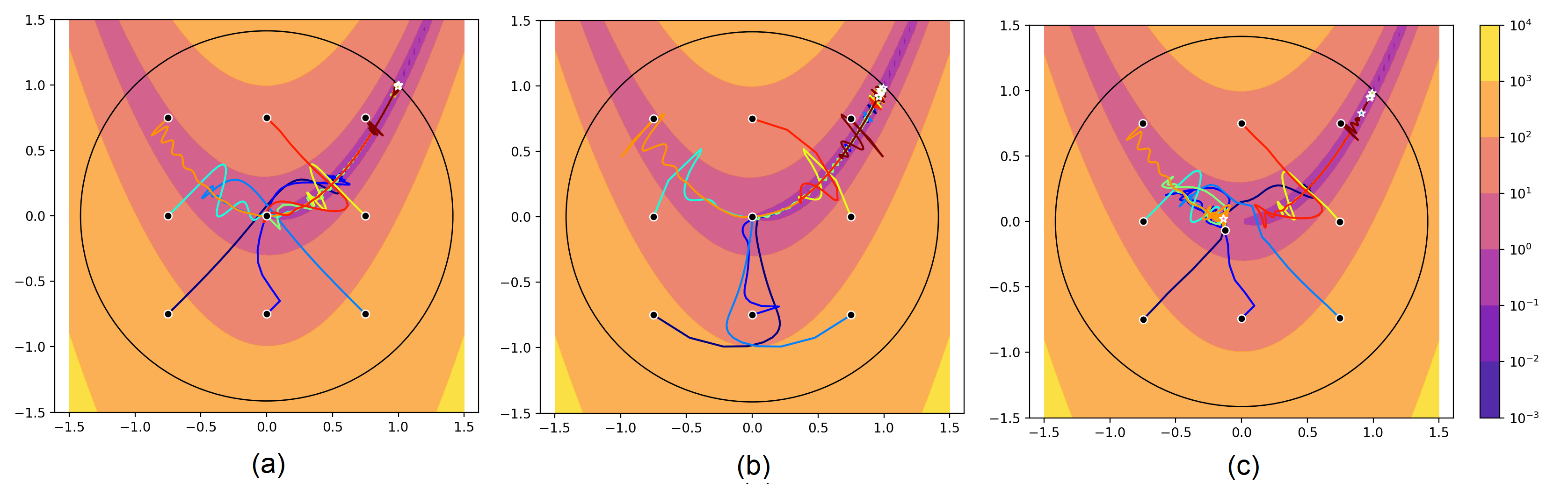
Figure 8: Optimization trajectories for the Rosenbrock function with quadratic constraints: (a) the central projection, (b) the hidden space $(r,s)$, (c) the projection neural network

Fig.9 shows the optimization trajectories for the non-convex Bird function from [19]:

$$\mathcal{L}_{Bird}(x)=sin(x_{2})e^{(1-cos(x_{1}))^{2}}+cos(x_{1})e^{(1-sin(x_{2}))^{2}}+(x_{1}-x_{2})^{2},$$ (57)

$$\Omega_{Bird}=\left\{x~{}|~{}(x_{1}+5)^{2}+(x_{2}+5)^{2}<25\right\}.$$ (58)

This function has four local minima in the region under consideration, two of which lie on the boundary of the set $\Omega_{Bird}$, which is depicted by the large black circle in Fig.9.

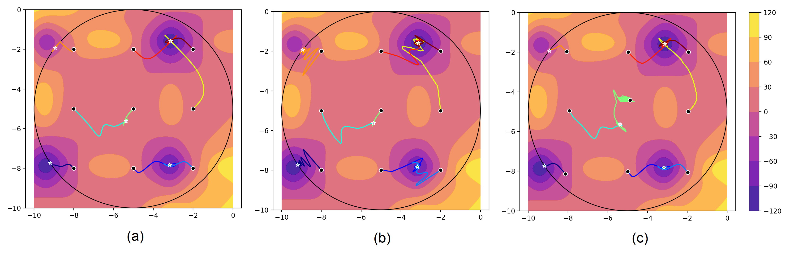
Figure 9: Optimization trajectories for the Bird function 57: (a) the central projection, (b) the hidden space $(r,s)$, (c) the projection neural network

4.2 A classification example

In order to illustrate capabilities of neural networks with the output constraints, consider the classification problem by using an example with the dataset Olivetti Faces taken from package “Scikit-Learn”. The dataset contains $400$ images of the size $64\times 64$ divided into $40$ classes. We construct a model whose output is a discrete probability distribution that is

$$f_{\theta}(z)\in\left\{x~{}|~{}x_{i}\geq 0,~{}\mathbf{1}^{T}x=1\right\}.$$ (59)

It should be noted that traditionally the softmax operation is used to build a neural network whose output is a probability distribution.

For comparison purposes, Fig.10 shows how the loss functions depend on the epoch number for the training and testing samples. Each neural network model contains $5$ layers of size $300$ and is trained using Adam on $5000$ epochs with the batch size $200$ and the learning rate $10^{-4}$ to minimize the cross entropy. Three types of final layers are considered to satisfy the constraints imposed on the probability distributions (59):

• Constraints means that the proposed layer of the neural network imposes constraints on the input $(r,s)$;

• Projection means that the proposed layer projects the input to the set of constraints;

• Softmax is the traditional softmax layer.

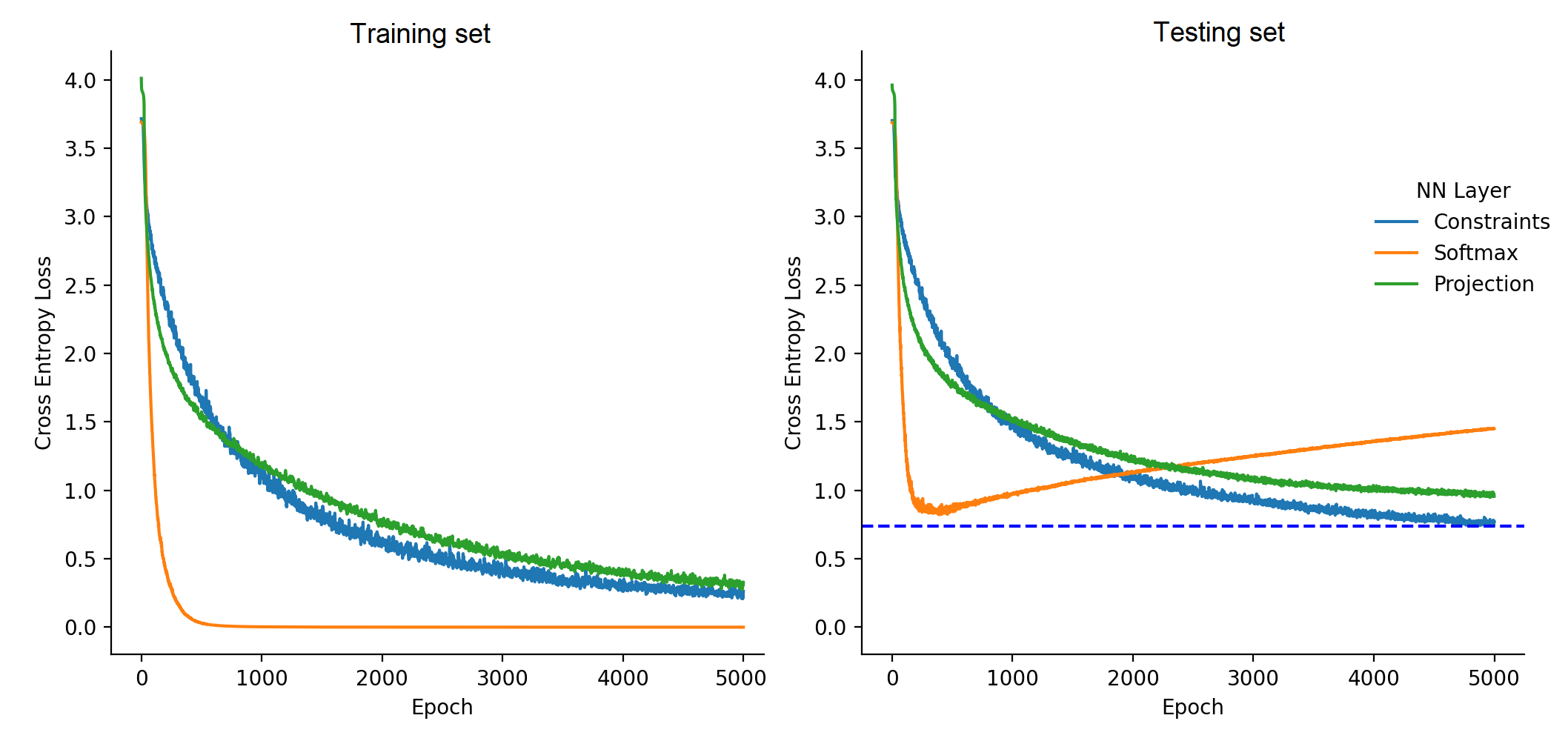
Figure 10: Comparison of cross entropy for different types of the final layer of the classification neural network

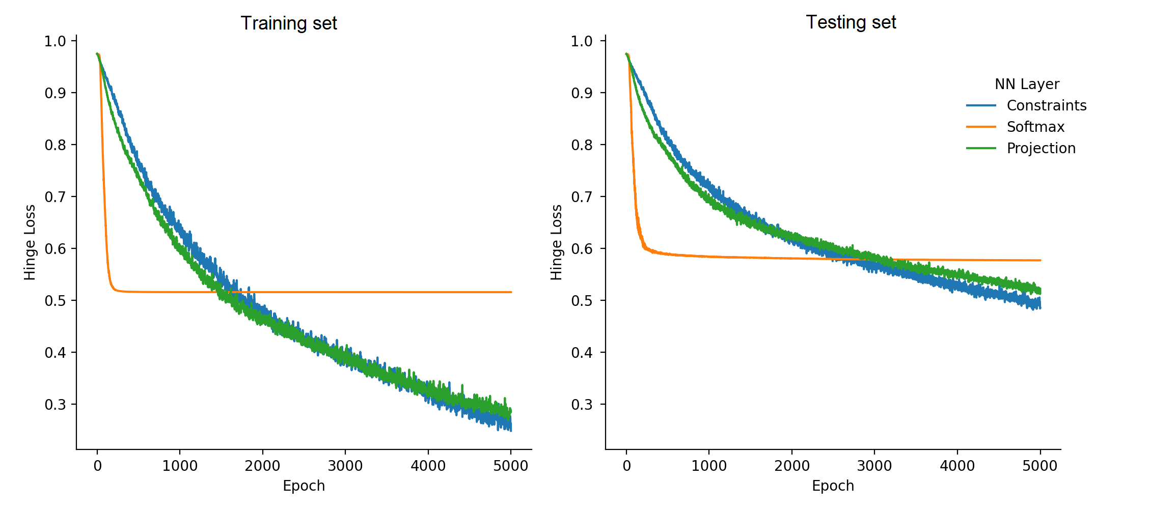
Figure 11: Comparison of “Hinge loss” for different types of the final layer of the classification neural network

The dotted line in Fig.10 denotes the minimum value of the loss function on the testing set. It can be seen from Fig.10 that all types of layers allow solving the classification problem. However, the proposed layers in this case provide slower convergence than the traditional softmax. This can be explained by the logarithm in the cross entropy expression, which is compensated by the exponent in the softmax. Nevertheless, the proposed layers can be regarded as a more general solution. In addition, it can be seen from Fig.11 that this hypothesis is confirmed if another loss function is used, namely “Hinge loss”. One can see from Fig.11 that the softmax also converges much faster, but to a worse local optimum.

In addition to the standard constraints (59), new constraints can be added, for example, upper bounds $\overline{p}_{i}$ for each probability $x_{i}$:

$$f_{\theta}(z)\in\left\{x~{}|~{}0\leq x_{i}\leq\overline{p}_{i},~{}\mathbf{1}^{T}x=1\right\}.$$ (60)

This approach can play a balancing role in training, by reducing the influence of already correctly classified points on the loss function. To illustrate how the neural network is trained with these constraints and to simplify the result visualization, a simple classic classification dataset “Iris” is considered. It contains only $3$ classes and $150$ examples. Three classes allow us to visualize the results by means of the unit simplex. In this example we set upper bounds $\overline{p}_{i}=0.75$ for $i=1,2,3$. Fig.12 shows the three-dimensional simplices and points (small circles) that are outputs of the neural network trained on 100, 500, and 1000 epochs. The neural network consists of $5$ layers of size $64$. Colors of small circles indicate the corresponding classes (Setosa, Versicolour, Virginica). It can be seen from Fig.12 that the constraints affect not only when the output points are very close to them, but also throughout the network training.

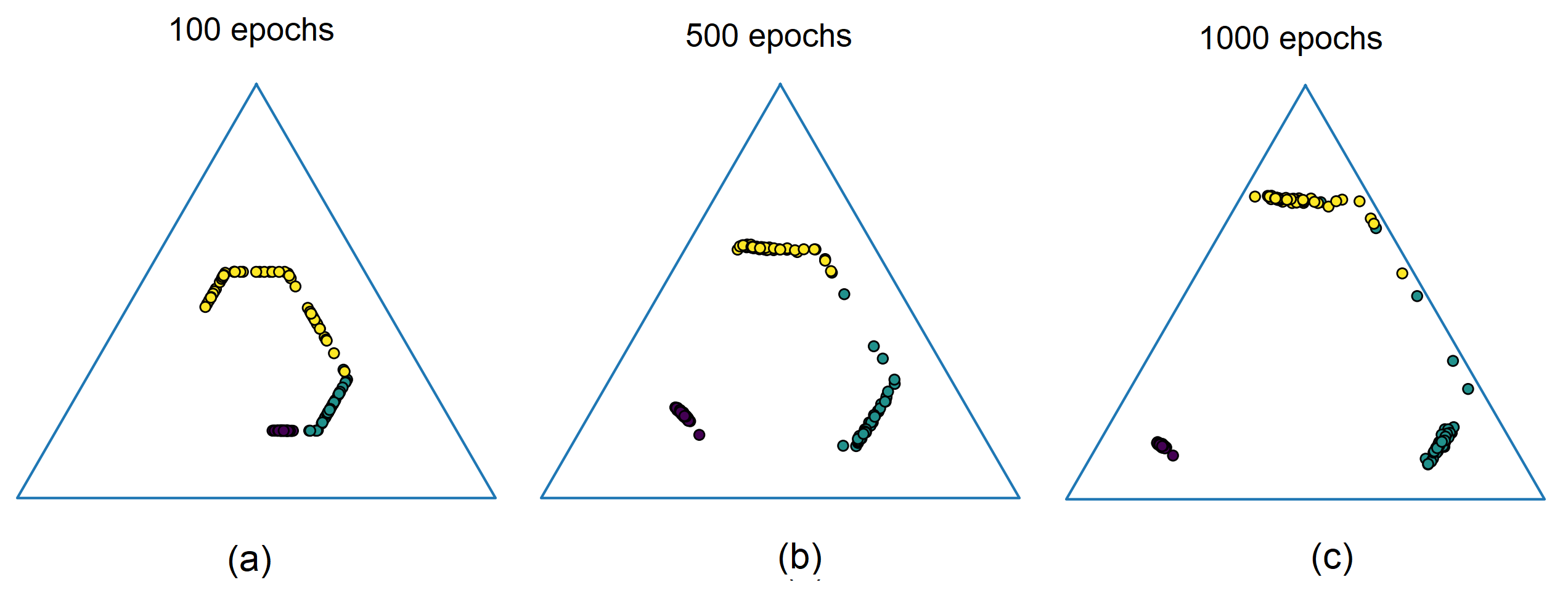
Figure 12: The class probability distributions by different number of epochs for training: (a) 100 epochs, (b) 500 epochs, (c) 1000 epochs,

5 Conclusion

The method, which imposes hard constraints on the neural network output values, has been presented. The method is extremely simple from the computational point of view. It is implemented by the additional neural network layer with constraints for output. Applications of the proposed method have been demonstrated by numerical experiments with several optimization and classification problems.

The proposed method can be used in various applications, allowing to impose linear and quadratic inequality constraints and linear equality constraints on the neural network outputs, as well as to constrain jointly inputs and outputs, to approximate orthogonal projections onto a convex set or to generate output vectors on a boundary set.

We have considered cases of using the proposed method under condition of the non-convex objective function, for example, the non-convex Bird function used in numerical experiments set of constraints. At the same time, the feasible set formed by constraints has been convex because the convexity property has been used in the proposed method when the point of intersection of the ray $r$ and one of the constraints was determined. However, it is interesting to extend the ideas behind the proposed method to the case of non-convex constraints. This extension of the method can be regarded as a direction for further research.

It should be pointed out that an important disadvantage of the proposed method is that it works with bounded constraints. This implies that the conic constraints cannot be analyzed by means of the method because the point of intersection of the ray $r$ with the conic constraint is in the infinity. We could restrict a conic constraint by some bound in order to find an approximate solution. However, it is interesting and important to modify the proposed method to solve the problems with the conic constraints. This is another direction for research.

There are not many models that actually realize the hard constraints imposed on inputs, outputs and hidden parameters of neural networks. Therefore, new methods which outperform the presented method are of the highest interest.

Another important direction for extending the proposed method is to consider various machine learning applications, for example, physics-informed neural networks which can be regarded as a basis for solving complex applied problems [20, 21]. Every application requires to adapt and modify the proposed method and can be viewed as a separate important research task for further study.

References

- [1] P. Marquez-Neila, M. Salzmann, and P. Fua. Imposing hard constraints on deep networks: Promises and limitations. In CVPR Workshop on Negative Results in Computer Vision, pages 1–9, 2017.
- [2] T. Frerix, M. Niessner, and D. Cremers. Homogeneous linear inequality constraints for neural network activations. In Proceedings of the IEEE/CVF Conference on Computer Vision and Pattern Recognition Workshops, pages 748–749, 2020.
- [3] Jay Yoon Lee, S.V. Mehta, M. Wick, J.-B. Tristan, and J. Carbonell. Gradient-based inference for networks with output constraints. In Proceedings of the AAAI Conference on Artificial Intelligence (AAAI-19), volume 33, pages 4147–4154, 2019.
- [4] P.L. Donti, D. Rolnick, and J.Z. Kolter. DC3: A learning method for optimization with hard constraints. In International Conference on Learning Representations (ICLR 2021), pages 1–17, 2021.
- [5] M. Brosowsky, F. Keck, O. Dunkel, and M. Zollner. Sample-specific output constraints for neural networks. In The Thirty-Fifth AAAI Conference on Artificial Intelligence (AAAI-21), pages 6812–6821, 2021.
- [6] B. Amos and J.Z. Kolter. Optnet: Differentiable optimization as a layer in neural networks. In International Conference on Machine Learning, pages 136–145. PMLR, 2017.
- [7] A. Agrawal, B. Amos, S. Barratt, S. Boyd, S. Diamond, and J.Z. Kolter. Differentiable convex optimization layers. Advances in neural information processing systems, 32:1–13, 2019.
- [8] Meiyi Li, S. Kolouri, and J. Mohammadi. Learning to solve optimization problems with hard linear constraints. IEEE Access, 11:59995–60004, 2023.
- [9] Randall Balestriero and Yann LeCun. Police: Provably optimal linear constraint enforcement for deep neural networks. In IEEE International Conference on Acoustics, Speech and Signal Processing (ICASSP), pages 1–5. IEEE, 2023.
- [10] Yuntian Chen, Dou Huang, Dongxiao Zhang, Junsheng Zeng, Nanzhe Wang, Haoran Zhang, and Jinyue Yan. Theory-guided hard constraint projection (HCP): A knowledge-based data-driven scientific machine learning method. Journal of Computational Physics, 445(110624), 2021.
- [11] F. Detassis, M. Lombardi, and M. Milano. Teaching the old dog new tricks: Supervised learning with constraints. arXiv:2002.10766v2, Feb 2021.
- [12] J. Hendriks, C. Jidling, A. Wills, and T. Schon. Linearly constrained neural networks. arXiv:2002.01600, Feb 2020.
- [13] G. Negiar, M.W. Mahoney, and A. Krishnapriyan. Learning differentiable solvers for systems with hard constraints. In The Eleventh International Conference on Learning Representations (ICLR 2023), pages 1–19, 2023.
- [14] K.C. Tejaswi and Taeyoung Lee. Iterative supervised learning for regression with constraints. arXiv:2201.06529, Jan 2022.
- [15] J. Kotary, F. Fioretto, and P. Van Hentenryck. Learning hard optimization problems: A data generation perspective. In 35th Conference on Neural Information Processing Systems (NeurIPS 2021), volume 34, pages 24981–24992., 2021.
- [16] J. Kotary, F. Fioretto, P. Van Hentenryck, and B. Wilder. End-to-end constrained optimization learning: A survey. In Proceedings of the Thirtieth International Joint Conference on Artificial Intelligence (IJCAI-21), pages 4475–4482, 2021.
- [17] B. Stellato, G. Banjac, P. Goulart, A. Bemporad, and S. Boyd. Osqp: An operator splitting solver for quadratic programs. Mathematical Programming Computation, 12(4):637–672, 2020.
- [18] H.H. Rosenbrock. An automatic method for finding the greatest or least value of a function. The Computer Journal, 3(3):175–184, 1960.
- [19] S.K. Mishra. Some new test functions for global optimization and performance of repulsive particle swarm method. Available at SSRN 926132, pages 1–24, 2006.
- [20] S. Kollmannsberger, D. D’Angella, M. Jokeit, and L. Herrmann. Physics-informed neural networks. In Deep Learning in Computational Mechanics: An Introductory Course, pages 55–84. Springer, Cham, 2021.
- [21] M. Raissi, P. Perdikaris, and G.E. Karniadakis. Physics-informed neural networks: A deep learning framework for solving forward and inverse problems involving nonlinear partial differential equations. Journal of Computational Physics, 378:686–707, 2019.