The CluMPR Galaxy Cluster-Finding Algorithm and DESI Legacy Survey Galaxy Cluster Catalogue

Abstract

Galaxy clusters enable unique opportunities to study cosmology, dark matter, galaxy evolution, and strongly-lensed transients. We here present a new cluster-finding algorithm, CluMPR (Clusters from Masses and Photometric Redshifts), that exploits photometric redshifts (photo-$z$’s) as well as photometric stellar mass measurements. CluMPR uses a 2-dimensional binary search tree to search for overdensities of massive galaxies with similar redshifts on the sky and then probabilistically assigns cluster membership by accounting for photo-$z$ uncertainties. We leverage the deep DESI Legacy Survey grzW1W2 imaging over one-third of the sky to create a catalogue of $\sim 300,000$ galaxy cluster candidates out to $z=1$, including tabulations of member galaxies and estimates of each cluster’s total stellar mass. Compared to other methods, CluMPR is particularly effective at identifying clusters at the high end of the redshift range considered ($z=0.75$–$1$), with minimal contamination from low-mass groups. These characteristics make it ideal for identifying strongly lensed high-redshift supernovae and quasars that are powerful probes of cosmology, dark matter, and stellar astrophysics. As an example application of this cluster catalogue, we present a catalogue of candidate wide-angle strongly-lensed quasars in Appendix C. The five best candidates identified from this sample include two known lensed quasar systems and a possible changing-look lensed QSO with SDSS spectroscopy. All code and catalogues produced in this work are publicly available (see Data Availability).

1 Introduction

Galaxy clusters are the most massive gravitationally bound structures in the universe, and therefore they are of great use in cosmology and astrophysics. One motivation for the creation of catalogues of clusters is to locate likely areas for observing strongly-lensed time-variable phenomena such as gravitationally lensed supernovae and quasars (Meyers et al., 2009). The observation of the time delays between the lensed images of variable phenomena, coupled with proper modeling of the lensing system, can provide an independent constraint on the Hubble-Lemaitre parameter (Refsdal, 1964). In 2015, multiple images of a supernova lensed by a galaxy cluster were observed (Kelly et al., 2015). Recently, the intermediate Palomar Transient Factory and its successor, the Zwicky Transient Facility (ZTF), have discovered several additional gravitationally lensed supernovae (Goobar et al., 2017, 2023). Meanwhile, programs to observe gravitationally lensed quasars are ongoing (Wong et al., 2020; Napier et al., 2023). Further observations of gravitationally lensed transients will lead to improved constraints on the nature of dark matter and the expansion of the universe.

Galaxy cluster catalogues have many other applications. As one example, they can be used to study the impact of clusters on the evolution of galaxies in their vicinity (Dressler, 1980). Gravitational magnification of background galaxies by galaxy clusters enables distant galaxies to be detected and studied at high resolution (e.g. Bayliss et al., 2014; Livermore et al., 2015; Johnson et al., 2017; Cornachione et al., 2018; Rivera-Thorsen et al., 2019; Ivison et al., 2020; Khullar et al., 2021; Bezanson et al., 2022). Furthermore, they can enable the detection and analysis of merging galaxy clusters, which are useful for constraining the dark matter scattering cross section (Wittman et al., 2023). Additionally, measurements of the apparent abundance of clusters can be a sensitive probe of cosmology (Haiman et al., 2001; Newman et al., 2002).

A purely photometric galaxy cluster-finding algorithm can take advantage of the large number of distant sources which can be observed using imaging. Conveniently, estimates of redshift and stellar mass can be obtained from the same photometric data. An algorithm which is optimally adapted for photometric observations will be essential for the upcoming generation of optical and infrared surveys at facilities such as Rubin Observatory (LSST Science Collaboration et al., 2009), Euclid Observatory (Euclid Collaboration et al., 2022), and the Nancy Grace Roman Telescope (Spergel et al., 2015), all of which will generate immense amounts of photometric data spanning many passbands.

The redMaPPer algorithm (Rykoff et al., 2014) is an example of a well-tested photometric galaxy cluster-finding algorithm. The redMaPPer algorithm relies on a red-sequence model to detect candidate galaxy clusters. Currently redMaPPer has been applied to data from the Sloan Digital Sky Survey Data Release 8 (SDSS DR8) (Aihara et al., 2011) and Dark Energy Survey Science Verification (DES SV) (Dark Energy Survey Collaboration et al., 2016). The redMaPPer SDSS DR8 catalogue contains 26,311 clusters over the redshift range 0.08<$z$<0.55 (Rykoff et al., 2014), while the redMaPPer DES SV contains 786 clusters from 0.2<$z$<0.9 (Rykoff et al., 2016).

Another well-tested cluster-finding algorithm was developed by Wen et al. (2009), henceforth WHL. This algorithm has been applied to SDSS (Wen et al., 2012; Wen & Han, 2015), Subaru Hyper Suprime-Cam (data: Aihara et al. (2018) and clusters: Wen & Han (2021)), and the Dark Energy Survey (data: The Dark Energy Survey Collaboration (2005) and clusters: Wen & Han (2022)). The WHL algorithm, just like the algorithm described in this paper, uses the "nearest-neighbor" technique to find neighboring galaxies, but it uses a deterministic slice in redshift rather than the probabilistic approach developed in this work.

The current largest galaxy cluster catalogue (Zou et al., 2021) was created by applying the Clustering by Fast Search and Find of Density Peaks (CFSFDP) algorithm (Rodriguez & Laio, 2014) to the Dark Energy Spectroscopic Instrument (DESI) Legacy Survey Data Release 8 (Dey et al., 2019). This work identified 540,432 galaxy cluster candidates reaching $z$=1 in the Dark Energy Spectroscopic Instrument Legacy Survey. Zou et al. (2021) use Sunyaev-Zel’dovich and X-ray data to calibrate total galaxy masses from richness-mass relations for this sample. Similarly to WHL, (Zou et al., 2021) use a deterministic redshift slice, rather than a probabilistic approach.

In this paper we present a new galaxy cluster-finding algorithm, which we call CluMPR (Clusters from Masses and Photometric Redshifts). This algorithm is designed to minimize the impact of projection effects caused by uncertainties in the photometric redshifts (photo-$z$’s) of individual galaxies. In this work, we optimize the details of this algorithm to enable the selection of a high-purity sample of high-stellar-mass clusters. These choices aid in selecting those galaxy cluster candidates which are most likely to cause strong lensing and help to optimize searches for transients associated with quiescent galaxies, while simultaneously minimizing contamination of the sample by lower-mass galaxy groups. Our algorithm determines total cluster stellar masses probabilistically by incorporating photometric redshift uncertainties and compensating for redshift-dependent mass incompleteness. We also provide a catalogue of cluster member galaxies and a catalogue of candidate gravitationally lensed quasars. Our catalogues are intended to complement existing galaxy cluster catalogues such as the ones created by Zou et al. (2021) and Yang et al. (2021) using DESI Legacy Survey data, and can also be used to compare the results of applying different algorithms to similar data.

This paper is organised as follows: In Section 2, we describe the data products we used to generate our galaxy cluster catalogue. Section 3.1 describes the CluMPR algorithm in detail. In Section 3.2, we describe our process for calibrating galaxy cluster parameters and assigning galaxy cluster member galaxies. In Section 4, we provide some summary graphs and data summarizing the characteristics of the CluMPR galaxy cluster catalogue. Finally, in Section 5 we summarize the results, applications, and potential future extensions of our work. The Data Availability section provides the publicly accessible locations of all data and code related to this paper, including the cluster catalogues and candidate lensed quasar catalogues. Appendices A and B describe details regarding the calibration of our algorithm; Appendix C describes a set of candidate gravitationally-lensed quasars we have identified; and Appendix D describes the columns of all catalogues assembled in this work. Throughout this paper, we assume a cosmology with $H_{0}=70\hskip 5.69054ptkm/s/Mpc,\hskip 5.69054pt\Omega_{m}=0.286,\hskip 5.69054pt\Omega_{\lambda}=0.714$ (Bennett et al., 2014).

2 Data

The DESI Legacy Imaging Surveys (Dey et al., 2019) has produced multi-band images of over a third of the sky (roughly 14,000 deg²) in three optical bands ($g,r,z$) and two infrared bands from WISE ($W1,W2$) (Wright et al., 2010). The optical component of this survey is composed of three separate programs: the Beijing-Arizona Sky Survey (BASS) (Zou et al., 2017), the Dark Energy Camera Legacy Survey (DECaLS) (Flaugher et al., 2015; Dey et al., 2019) with supplementary data from the Dark Energy Survey (The Dark Energy Survey Collaboration, 2005), and the Mayall z-band legacy survey (MzLS) (Silva et al., 2016). A full description of the Legacy Imaging Surveys is available at Dey et al. (2019). The primary purpose of the DESI Legacy Imaging Surveys is to obtain targets for spectroscopic follow-up with DESI (Dark Energy Spectroscopic Instrument, DESI Collaboration et al. (2022)). We obtained photometric redshifts for our analysis from Zhou et al. (2021) and stellar mass estimates from Zhou et al. (2023).

We apply several photometric cuts to select galaxies for our analysis with good measurements of photometric redshifts and stellar masses and with as little contamination from stars as possible. We restrict ourselves to objects with

1. z magnitude < 21 (photo-z’s are only reliable for z band magnitude < 21, see Zhou et al. (2021)),

2. Either Gaia photometric mean magnitude > 19, Gaia astrometric excess noise > 10^0.5, or Gaia astrometric excess noise = 0 (in order to remove stars),

3. TYPE != PSF (setting TYPE to exclude point spread function objects removes stars and quasars while keeping the vast majority of galaxies, since bright galaxies are able to be resolved)

4. Photometric redshift > 0.01 (due to photo-z and de-blending unreliability at low z)

We restrict ourselves to galaxies with a known stellar mass from Zhou et al. (2023). These are objects which have valid photometry in the $g$, $r$, $z$, W1, W2 bands and satisfy the stellar rejection cut of $r-W1>1.75\times(r-z)-1.1$. We limit ourselves to galaxies with a DESI legacy Survey DR9 bitmask value 0 or 4096, which correspond respectively to unmasked galaxies and SGA galaxies (Moustakas et al., 2021). The photometric redshifts and the stellar masses were estimated using the Random Forest algorithm trained on legacy survey photometry and a carefully vetted training set of spectroscopic redshifts and stellar population synthesis-based mass estimates. The errors on the photometric redshifts were generated by perturbing the original photometry and using the spread in the distributions of the predicted redshifts as a measure of the error. Detailed descriptions of the methods and catalogues can be found in Zhou et al. (2021, 2023).

Note: throughout this text, a "sweep" refers to a continuous subsection of DESI Legacy survey photometry data which is contained in a single file.

3 Methods

3.1 CluMPR Algorithm Overview

The CluMPR algorithm is comprised of four essential steps:

1. Potential Cluster Center Selection: Select galaxies with large stellar mass.

2. Membership Probability Calculation: For each potential cluster center galaxy, evaluate the expected number of neighbouring galaxies within a cylinder oriented lengthwise along the line of sight ($z$) direction (see Fig.  1). In the direction of the cylinder’s radius, membership is determined deterministically using a binary search tree. Along the z direction, membership is determined probabilistically based on photo-$z$ uncertainties.

3. Richness Thresholds: Keep potential cluster center galaxies with a significant excess of neighbouring galaxies (this is equivalent to defining a galaxy cluster by setting a minimum richness).

4. Aggregation: neighbouring potential cluster center galaxies are aggregated and the galaxy with the highest local stellar mass is chosen as the cluster center.

This cylinder-based method is a probabilistic variant of the widely-used (deterministic) "counts-in-cylinders" technique (Hogg et al., 2004; Blanton et al., 2006; Kauffmann et al., 2004; Barton et al., 2007; Berrier et al., 2011). The individual steps of the CluMPR algorithm are explained in greater detail below.

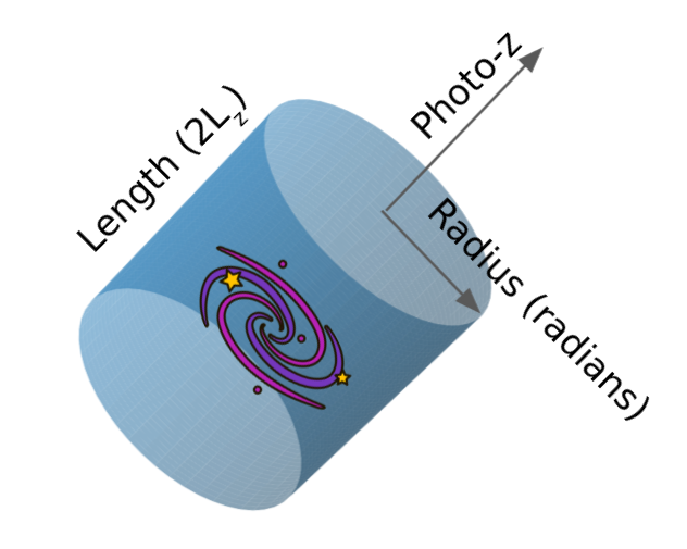
Figure 1: Search cylinder for CluMPR algorithm, oriented lengthwise along redshift (line-of-sight) direction and centered on the potential cluster center galaxy.

3.1.1 Potential Cluster Center Selection

Potential cluster center galaxies are chosen from the general pool of galaxies based on a minimum stellar mass threshold. We set this minimum stellar mass threshold to be log(stellar mass) > 11.2 [log($M_{\odot}$)]. This mass threshold was chosen based on visual inspection of galaxy clusters (we chose to minimize the fraction of low-mass groups and spurious detections in order to create a high-purity cluster catalogue, but this mass threshold can be lowered if a lower-purity catalogue is desired).

3.1.2 Membership Probability Calculation

For each potential cluster center galaxy chosen in 3.1.1, we count the number of neighbours in a cylinder oriented lengthwise along the $z$ direction and centered on the potential cluster center galaxy.

First, galaxies are selected within a fixed physical radius of the cluster center galaxy (we use three radii: 1 Mpc, 0.5 Mpc, and 0.1 Mpc. The significance of these radii is explained in the subsequent sections). This first step is accomplished using a binary search tree; our implementation uses the cKDTree algorithm from the SciPy Python package (Virtanen et al., 2020). In order to avoid propagating photo-$z$ errors into the angular positions of galaxies, we perform this step using angular coordinates. The physical radius is calculated in angular coordinates using the following equation:

$$\mathrm{R_{ang}}(z)=(\mathrm{R_{phys}})\frac{1+z}{D(z)},$$ (1)

where $\mathrm{R_{ang}}$ is the radius in angular coordinates (radians), $\mathrm{R_{phys}}$ is the physical radius in megaparsecs, $z$ is the redshift, and $D(z)$ is the comoving distance given by

$$D(z)=\int_{0}^{z}\frac{dz^{\prime}}{H(z^{\prime})},$$ (2)

where $H(z^{\prime})$ is the Hubble-Lemaitre parameter. A graph of Equation 1 for $R_{phys}=1Mpc$ is shown in Figure 2. For each potential cluster center galaxy, we calculate the radius using Equation 1 and the photo-$z$ of the cluster center galaxy. To ensure equal area projection of angular coordinates, we use a sinusoidal (Sanson–Flamsteed) projection. To avoid issues associated with very small values for angular coordinates, we add an offset of 50 radians to each coordinate.

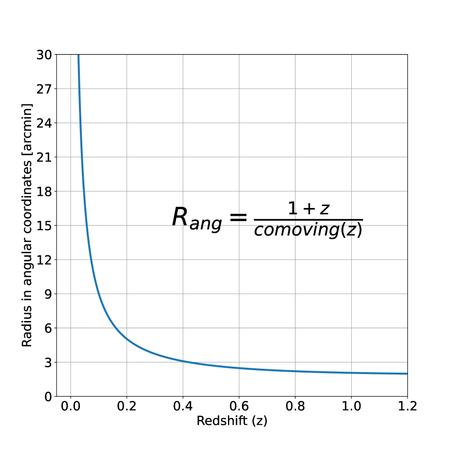
Figure 2: Search cylinder radius in angular coordinates (radians) as a function of redshift. Obtained from Equation 1.

Next, to determine cluster membership along the z-direction (lengthwise along the cylinder), we apply a redshift cut based on the photo-$z$ of the cluster center galaxy. The length of this cut (the half-length of the cylinder) is given by

$$L_{z}(z)=2\overline{\sigma_{z}},$$ (3)

where $\overline{\sigma_{z}}$ is the interpolated redshift-dependent binned average of the photo-$z$ error for all galaxies. To train our model for $\overline{\sigma_{z}}$, we used 100 bins between the lowest and highest photo-$z$’s in the training sample; we limited $\overline{\sigma_{z}}$ to 0.1 at high z. We used 20 randomly-selected DESI Legacy Survey sweep files (10 from North (BASS/MzLS) and 10 from South (DECaLS)) as our training samples. The linearly-interpolated trained results for $\overline{\sigma_{z,north}}$ and $\overline{\sigma_{z,south}}$ are shown in Figure 3. $L_{z}$ is significantly larger than the true redshift extent of a galaxy cluster at all redshifts, which means that a probabilistic approach to cluster membership along the z direction is required.

We use $L_{z}$ to determine the probability that a galaxy within the search cylinder’s radius is a true member of the cluster (that is, the probability that it is truly within the cylinder). In order to determine this probability, we use statistical resampling, whereby we create many realizations of each galaxy’s potential true redshift; these realizations are drawn from a Gaussian distribution centered on the photo-$z$ of the galaxy and with a standard deviation equal to the photo-$z$ error for the galaxy. The percentage of these redshift realizations falling within $L_{z}$ of the cluster center galaxy’s photo-$z$ is the membership probability.

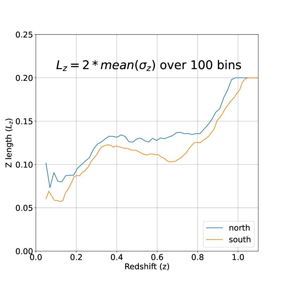
Figure 3: Interpolated redshift-dependent binned average of the photo-$z$ error as a function of redshift. This is the half-length of the search cylinder. Note that $L_{z}$ is limited to 0.2. South refers to the DECaLS survey data, while north refers to the data from BASS and MzLS.

3.1.3 Richness Thresholds

In order to identify galaxy clusters among the potential cluster center galaxies selected in Step 3.1.1, we apply a threshold for the minimum number of galaxies that must be located within the galaxy’s search radius. This is equivalent to defining what is a galaxy cluster by setting a minimum richness threshold. We apply a redshift-dependent threshold to both the 1-Mpc cylinder and the 0.5-Mpc cylinder; only potential cluster center galaxies that satisfy both thresholds are kept as galaxy clusters. For the 1-Mpc cylinder, the threshold we used is

$$T_{1}>\overline{N}+1.8\sigma_{N},$$ (4)

and for the 0.5-Mpc cylinder, the threshold we used is

$$T_{0.5}>\overline{N}+1.2\sigma_{N},$$ (5)

where $\overline{N}$ is the redshift-binned average number of galaxies within a cylinder of that size, and $\sigma_{N}$ is the redshift-binned standard deviation of the number of galaxies within a cylinder of that size. These thresholds were chosen based on visual inspection for purity of resulting galaxy clusters. We assume a Poisson distribution for the number of galaxies within a cylinder, which allows us to define

$$\sigma_{N}=\sqrt{\overline{N}}.$$ (6)

The richness threshold is interpolated linearly as a function of $z$; the results of this interpolation are shown in Figure 4. The training data for these thresholds are the same as in Section 3.1.2, and the redshift bins are $z$=0.01 apart with a width of $z$ = 0.05, ranging from the lowest to the highest photo-$z$ in the training samples.

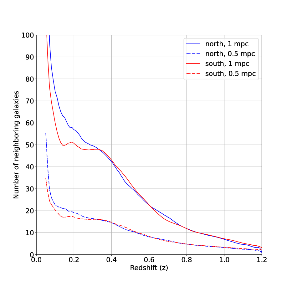
Figure 4: Interpolated redshift-dependent thresholds for 1-Mpc and 0.5-Mpc cylinders. South refers to the DECaLS survey data, while north refers to the data from BASS and MzLS.

3.1.4 Aggregation

In order to remove duplicate galaxy clusters (several center galaxy candidates for one galaxy cluster), we use a similar method to Section 3.1.2, except that the radius of the aggregation cylinder is 1.5 Mpc, and the $L_{z}$ cutoff is not done probabilistically.

First, all cluster central galaxies are sorted by (uncorrected, see 3.2.2) total stellar mass within a 0.5 Mpc radius. Beginning with the cluster central galaxies with the greatest 0.5 Mpc stellar mass, neighbouring cluster central galaxies within R=1.5 Mpc and $L_{z}$ are labelled as belonging to the same cluster. The galaxy with the greatest (uncorrected) total stellar mass within a 0.1 Mpc radius is then chosen as the cluster center galaxy.

3.1.5 Data Cleaning

We apply several flags to our galaxy clusters to remove poor objects. First, galaxy clusters within 0.285 degrees of the edge of the DESI Legacy Survey footprint are flagged. We flag clusters near large foreground galaxies from the Siena Galaxy Atlas (SGA) (Moustakas et al., 2021). Our criteria for the SGA galaxies are either

1. D26 > 1.5,

2. R_MAG_SB24 < 13.5, R_MAG_SB24>0, and Z_LEDA <0.05

Some of these flagged objects are false detections (which are mostly due to failed de-blending of foreground galaxies), while others are real galaxy clusters with significant foreground contamination which could affect the photo-$z$ and stellar mass estimates. Finally, we remove all clusters located in the isolated strips of the DESI Legacy Survey footprint with declination < -10.3 degrees and 110 < Right ascension (degrees) < 250. We provide a catalogue which includes all flagged objects as a supplement to the main CluMPR catalogue.

3.2 Cluster Parameters

Each galaxy cluster in our catalogue is labelled with a unique "gid", which is created from the cluster center galaxy’s coordinates using the following formula:

round(RA, 6 decimals) * $10^{16}$ + round(DEC + 90, 6 decimals) * $10^{6}$

where RA is right ascension and DEC is declination (both in degrees). Each galaxy cluster has a richness estimate (number of neighbours) for the 1 Mpc, 0.5 Mpc, and 0.1 Mpc search radii. The "gid" is necessary to identify the galaxy cluster members described in Section 3.2.3. Additionally, we provide galaxy cluster parameters for redshift and mass as described below.

3.2.1 Probability and Mass Weighting of Cluster Redshift Parameters

For each galaxy cluster we calculate the following redshift parameters (in addition to providing the photo-$z$ information for the cluster center galaxy):

1. Average photo-$z$ of all galaxy cluster member galaxies

2. Average photo-$z$ of all galaxy cluster member galaxies (weighted by membership probability)

3. Average photo-$z$ of all galaxy cluster member galaxies (weighted by galaxy stellar mass times membership probability)

4. Standard error of photo-$z$ of all galaxy cluster member galaxies

5. Standard error of photo-$z$ of all galaxy cluster member galaxies (weighted by membership probability)

6. Standard error of photo-$z$ of all galaxy cluster member galaxies (weighted by galaxy stellar mass times membership probability)

The average photo-$z$ estimates for the clusters are biased high, particularly for certain galaxy clusters at low z. This is due to systematic errors caused by the higher probability of a line-of-sight galaxy at high z falling within the cylinder of the cluster (as high-z galaxies have larger photo-$z$ errors on average). This bias is further amplified by volume effects: the angular diameter of the cylinder encloses a larger volume at high z. In this work, we do not attempt to correct for this systematic error. For this reason, we recommend using the photo-$z$ of the cluster center galaxy as a relatively unbiased estimate of the galaxy cluster redshift. Discrepancies between different estimates for the cluster’s average photo-$z$ are useful for identifying individual clusters with significant line-of-sight effects which may affect cluster parameters. The standard error estimates are (to first order) independent of the systematic error described above, so they can be used as an approximation for the random error uncertainty in cluster redshift. If more robust estimates (such as Hodges-Lehmann) for cluster redshift and uncertainty are desired, they can be calculated from the cluster membership catalogues (see Section 3.2.3).

3.2.2 Cluster Richness and Stellar Mass Estimates

We provide a background-corrected richness estimate which is background-corrected but not corrected for survey incompleteness. This richness is calculated by summing the membership probabilities of the galaxy cluster member galaxies and then subtracting the average galaxy background from this sum. The calculation of the average galaxy background is described in Appendix A.

We determine galaxy cluster stellar masses by summing the membership probability-weighted stellar masses of all cluster member galaxies within the 1 Mpc, 0.5 Mpc, and 0.1 Mpc search radii. We exclude galaxies with a mass below a threshold described in Appendix B (Equation 9). We then subtract the average galaxy stellar mass background, which is described in Appendix A. Finally, we apply a redshift-dependent correction factor which compensates for redshift-dependent mass incompleteness. This factor is described in Appendix B; the result is an incompleteness-corrected cluster stellar mass containing all cluster members above log($M_{\star}/M_{\odot}$) = 10.

3.2.3 Cluster Membership

For every galaxy cluster, we have compiled a list of member galaxies (galaxies whose membership probability > 0). For galaxies which are found to belong to more than one galaxy cluster, we assign the galaxy cluster for which there is the highest probability of membership. For each galaxy cluster, the cluster member galaxies can be identified using the "gid" parameter (see Section 3.2). The membership probability for the cluster member galaxies provided in the membership catalogue is not the same as the probability defined in Section 3.1.2. Instead, it is the probability of the member galaxy having a true redshift equal to the photo-$z$ of the galaxy cluster’s central galaxy, assuming a Gaussian distribution centered on the member galaxy’s redshift with a standard deviation equal to that member galaxy’s photo-$z$ error.

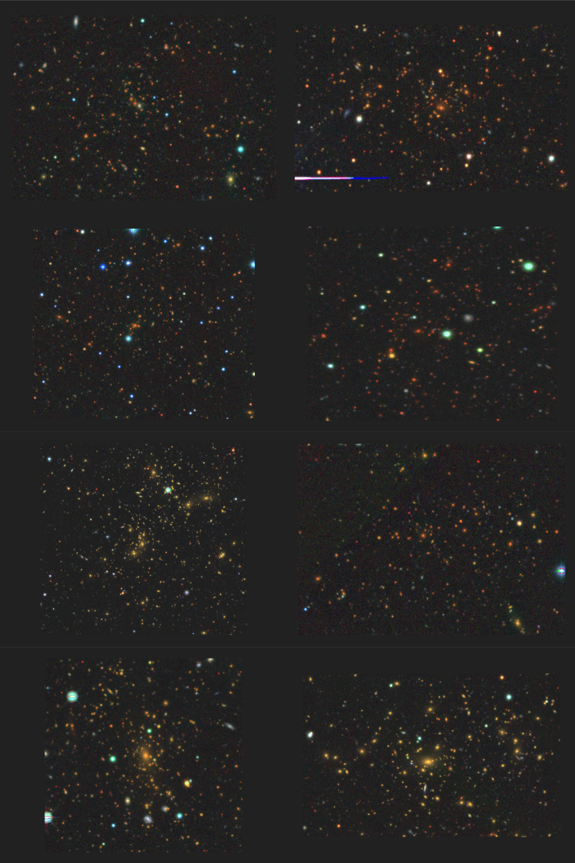
Figure 5: Examples of galaxy clusters found by the CluMPR algorithm in the DESI Legacy Survey imaging. The redshifts of these clusters range from $z$ = 0.305 (left column, third row) to $z$ = 0.707 (right column, second row).

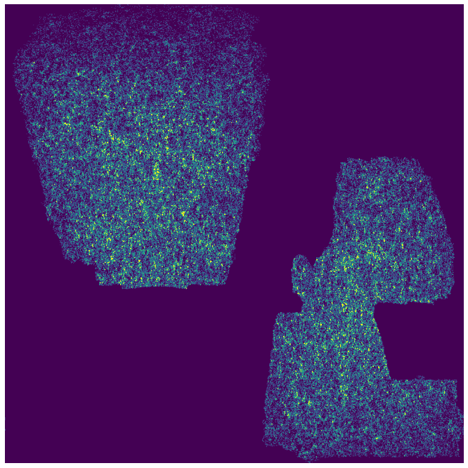
Figure 6: Density of galaxy clusters found by the CluMPR algorithm in the DESI Legacy Survey on the sky.

4 Results

The CluMPR algorithm has returned 309115 candidate galaxy clusters from 0.1<$z$<1. Galaxy clusters with $z$<0.1 are excluded as our algorithm is not optimised for those objects, which are frequently contaminated by poorly deblended foreground galaxies. Figure 5 shows a few examples of galaxy clusters from our catalogue at various redshifts. The distribution of our catalogue’s galaxy clusters on the sky is shown in Figure 6. Figure 7 shows the redshift and stellar mass distribution of CluMPR clusters. For 0.1<$z$<0.3, the sample is volume-limited; above $z$=0.3, the sample is limited by incompleteness. The stellar mass correction factor causes the stellar mass distribution to remain relatively flat across z. Low-mass galaxy clusters are excluded by our thresholds and incompleteness at high z, while high mass galaxy clusters are volume-limited. The rise in high-stellar-mass clusters at $z$<0.3 indicates that the catalogue is volume-limited for those redshifts; the decline in high-stellar-mass clusters at z > 0.6 may be due to limits imposed by structure formation (relations between our stellar mass estimates and total halo mass must be established to verify this cause).

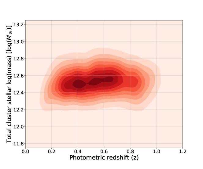
Figure 7: 1-Mpc total stellar mass vs photo-$z$ for galaxy clusters found by the CluMPR algorithm in the DESI Legacy Survey imaging. Cluster stellar masses have been background-subtracted and corrected for incompleteness with Stellar Mass Correction Factor. The top histogram shows the redshift distribution of CluMPR clusters with the redshift distributions of Zou et al. (2021) (black) and redMaPPer (red) overplotted. The right side histogram shows the stellar mass distribution of CluMPR clusters.

4.1 Cross-matching with Zou et al. 2021

The galaxy cluster catalogue described in Zou et al. (2021) was compiled using the same DESI Legacy Survey data as our catalogue, so cross-matching the catalogues yields a direct comparison of our implementation of CluMPR with the implementation of the CFSFDP algorithm by Zou et al. (2021). For cross-matching, we apply a simple 2-dimensional cross-matching which ignores line-of-sight coincidence. The radius for determining a match was 5 arcminutes, which is sufficient to handle most differences in the choice of cluster center galaxy while minimizing spurious matches. We found that this radius worked reasonably well at all redshifts.

Overall, Zou et al. (2021) found 85.4% of the galaxy clusters identified by CluMPR above $z$=0.1. Figure 8 shows the stellar mass within 1 Mpc for CluMPR galaxy clusters as a function of redshift; color indicates the fraction of CluMPR clusters found by Zou et al. (2021) Between $z$=0.1 and $z$=0.75, there is broad agreement between CluMPR and Zou et al. (2021) on high-richness objects, but Zou et al. (2021) miss some low-richness candidates identified by CluMPR. At $z$>0.75, Zou et al. (2021) miss a large fraction of clusters identified by CluMPR, including high-mass clusters. Visual inspection of the high-$z$ clusters missed by Zou et al. (2021) indicates a high fraction of true galaxy clusters. The likely reason for Zou et al. (2021) missing these objects is that they use a minimum richness of 10 which is not corrected for incompleteness; at high redshift, many clusters will have a low observed richness. This effect is best illustrated by Figure 9, which shows the 1-Mpc CluMPR richness as a function of redshift; color indicates the fraction of CluMPR galaxies found by Zou et al. (2021). At low-$z$, the CluMPR richness threshold for a cluster is relatively high, but it drops rapidly with $z$; by $z~{}0.75$, the richness threshold falls below 10, and the fraction of galaxy clusters recovered by Zou et al. (2021) falls to  0.5. CluMPR is able to maintain relatively high purity at high z despite the low richness threshold by using high-stellar mass galaxies as a reliable starting point for finding galaxy clusters, which works even in the absence of a large number of cluster member galaxies.

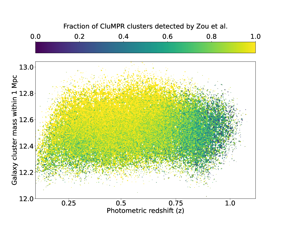
Figure 8: 1-Mpc total stellar mass vs photo-$z$ for galaxy clusters found by the CluMPR algorithm in the DESI Legacy Survey imaging (same as Figure 7). Color represents the fraction of CluMPR clusters found by Zou et al. (2021) The catalogue by Zou et al. (2021) has broad agreement on high mass clusters.

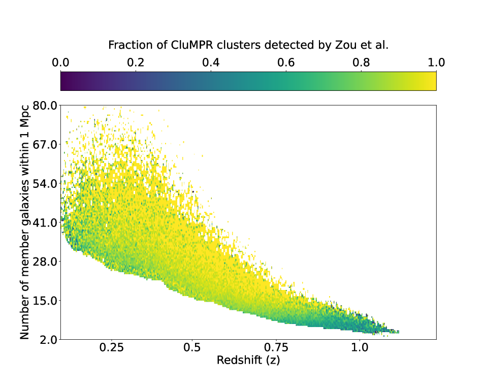
Figure 9: 1-Mpc richness (expected number of neighbours) vs photo-$z$ for galaxy clusters found by the CluMPR algorithm in the DESI Legacy Survey imaging. Color represents the fraction of CluMPR clusters found by Zou et al. (2021). The lower bound on richness is set by the thresholds in Section 3.1.3 (compare Figure 4).

Overall, CluMPR finds 58.9% of the galaxy clusters identified by Zou et al. (2021); however, this percentage increases to 87.1% if one limits the Zou et al. (2021) sample to clusters with richness > 30. Figure 10 shows 1 Mpc richness for Zou et al. (2021) galaxy clusters as a function of redshift; color indicates the fraction of CluMPR clusters found by Zou et al. (2021) As in Figure 8, there is broad agreement on high-richness objects. At all redshifts, CluMPR does not find most of the low-richness galaxy clusters identified by Zou et al. (2021) Thus, it is likely that the CluMPR sample is better optimised for detecting high-mass clusters with high purity. An implementation of CluMPR with lower richness thresholds would likely yield results more similar (for $z<0.75$) to Zou et al. (2021).

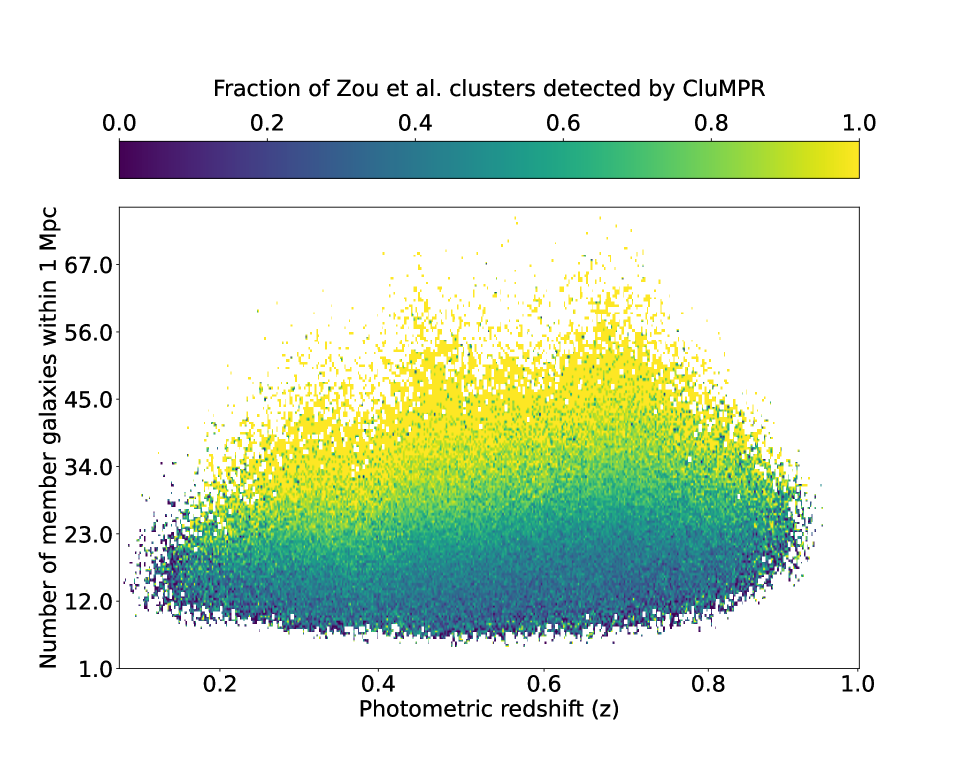
Figure 10: 1-Mpc richness (expected number of neighbours) vs photo-$z$ for galaxy clusters found by Zou et al. (2021) in the DESI Legacy Survey imaging. Color represents the fraction of CluMPR clusters found by Zou et al. (2021).

4.2 Cross-matching with SDSS redMaPPer and SDSS spectroscopy

Both CluMPR and Zou recover most of the objects from the SDSS redMaPPer cluster catalogue. Using the 5 arcminute radius cross-matching described in Section 4.1, CluMPR recovers 95% of redMaPPer clusters, while Zou et al. (2021) recover 99% of redMaPPer clusters. Figure 11 shows the 1-Mpc cluster stellar mass vs redMaPPer richness. As redMaPPer richness is known to be correlated with total cluster mass (Simet et al., 2017), the observed correltion between CluMPR stellar mass and redMaPPer richness is a strong indicator that CluMPR stellar masses are correlated with total cluster mass.

We provide spectroscopic redshifts for galaxies whose spectra have been obtained by the Sloan Digital Sky Survey (SDSS) (Blanton et al., 2017). Figure 12 shows the residuals between SDSS spectra and three photometric estimates for cluster redshift from CluMPR, as well as the residuals for redshift estimates by redMaPPer and Zou et al. (2021) The bias for average redshifts obtained by CluMPR is caused by line-of-sight galaxies falling within the cluster; this bias is increased when photo-$z$ errors are systematically over-estimated, as this creates an artificially long cylinder and increases the likelihood for galaxies to fall within the cylinder. Zhou et al. (2021) indicate that photo-$z$ errors are indeed overestimated, so this bias would be reduced with an improved redshift uncertainty quantification. However, our algorithm is still able to reduce the bias by weighting the cluster members by mass*probability (shown, middle right) or just probability (not shown). This indicates that our stellar mass and richness estimates are likely also improved by our probabilistic approach.

Figure 11: 1-Mpc cluster stellar mass vs redMaPPer richness. The redMaPPer catalogue does not have clusters below richness = 20. The cluster stellar mass has been background-subtracted and corrected for incompleteness with Stellar Mass Correction Factor. There is a clear correlation between CluMPR cluster stellar mass and redMaPPer richness, which indicates that CluMPR stellar masses are likely correlated with total cluster mass as well.

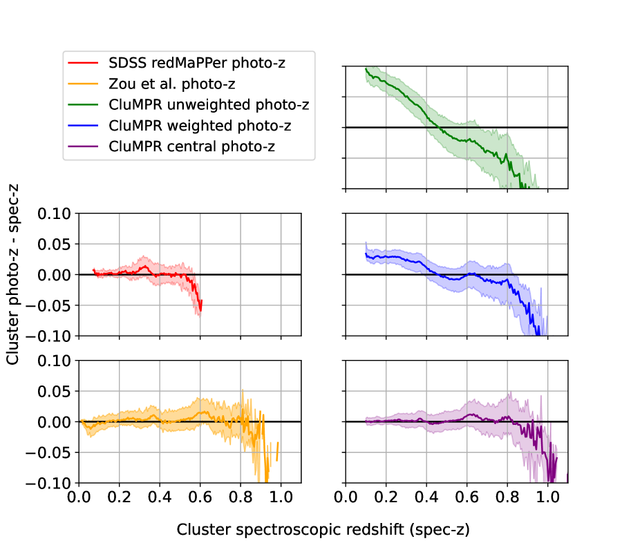
Figure 12: Residuals between SDSS spectroscopic redshifts and various estimates of cluster redshift from photo-$z$’s. Plotted intervals contain 68.2% of clusters. Our catalogue offers several redshift estimates; the photo-$z$ of the cluster central galaxy is least biased (bottom right). The plotted weighted average (middle right) uses mass*probability weighting, which reduces bias compared to an unweighted average redshift (top right). We include a catalogue of the member galaxies for all clusters, which can be used to calculate alternative estimates of the cluster redshift. All plotted redshift estimates underestimate spectroscopic redshift near the high-$z$ limit due to sharply decreasing galaxy counts at increasing redshifts (attenuation bias, see Freeman et al. 2009), which leads to a redshift estimate for the cluster central galaxy which is biased low.

5 Conclusions

We have used the CluMPR algorithm to identify over 300,000 galaxy clusters using the DESI Legacy Survey imaging data. This algorithm provides incompleteness-corrected stellar masses for each cluster as well as cluster membership probabilities for potential member galaxies. Our catalogue shows good correspondence to previous catalogues such as Zou et al. (2021) and SDSS redMaPPer (Rykoff et al., 2014) in overlapping regimes, and visual inspection of the detected galaxy clusters indicates that our methods have produced a high-purity sample.

CluMPR has several advantages over non-probabilistic cluster-finding algorithms such as the WHL algorithm (Wen et al., 2009) or the CFSFDP algorithm (Rodriguez & Laio, 2014) as used by Zou et al. (2021). As an example, for strong lensing searches, CluMPR enables us to select a sample of high-stellar-mass clusters that simultaneously has high purity. Higher-redshift lensing searches are further enhanced as CluMPR is able to more easily identify galaxy clusters at higher $z$ ($z>0.75$), a regime where smaller number of cluster galaxies will be brighter than magnitude thresholds and hence apparent richnesses will be lower. However, by using the presence of a single massive galaxy ($log(M_{\star})>11.2$) as a signpost to reliably anchor cluster assignments, CluMPR is able to still identify clusters with high purity even when the apparent richness drops. In contrast to red-sequence-based algorithms such as redMaPPer (Rykoff et al., 2014), CluMPR includes all potential galaxy cluster members in its search, which leads to a more complete member sample. This difference will become more relevant for deeper surveys, as we would expect a higher fraction of cluster members which are not on the red sequence at high $z$ (Schechter, 1976; Dahle et al., 2013). Finally, our probabilistic approach to cluster membership reduces systematic errors in cluster properties caused by the incorporation of infalling foreground or background galaxies.

The CluMPR DESI Legacy Survey catalogue can now be used by astronomers to search for strongly-lensed time-variable phenomena (such as supernovae and quasars) as well as other applications. As an example of how this catalogue may be used, we provide a supplementary catalogue of candidate lensed quasars in Appendix C. The five best candidates identified from this sample include two known systems and a possible changing-look lensed QSO with SDSS spectroscopy. The CluMPR DESI Legacy Survey catalogue can also be used for galaxy evolution studies and to search for merging galaxy clusters.

The CluMPR sample could be made more useful for cosmological studies by calibrating the relationship between the cluster stellar masses we have measured and total cluster masses as derived from Sunyaev-Zel’dovich, X-ray, or weak lensing measurements. Future datasets from Rubin Observatory (LSST Science Collaboration et al., 2009), Euclid Observatory (Euclid Collaboration et al., 2022), the Nancy Grace Roman Telescope (Spergel et al., 2015), and other next-generation surveys will provide another application for the CluMPR algorithm. These projects should provide higher-precision photometric redshifts and useful stellar mass measurements for objects several magnitudes fainter than the Legacy Survey objects studied here. As a result, these deep imaging surveys could extend CluMPR’s reach to $z=2$ and beyond.

Data Availability

The CluMPR galaxy cluster catalogue and cluster member galaxy catalogue are currently publicly available at DOI:10.5281/zenodo.8157752. The candidate lensed quasar catalogue is publicly available atDOI:10.5281/zenodo.8164870. Descriptions of each catalogue’s columns can be found in Appendix D.

These catalogues are also available to NERSC users at global/cfs/cdirs/desi/users/mjyb16/CLUMPR_DESI_2023. The main catalogue can be found in the folder clean_data, the extended catalogue including flagged objects can be found in the folder unclean_data, catalogues of cluster member galaxies can be found in the folder members, and the candidate lensed quasar catalogues can be found in the folder lensed_qso_candidates.

Code from this project can be found on GitHub.

Appendix A Galaxy Count and Stellar Mass Backgrounds

To determine the backgrounds, we run the CluMPR algorithm as described in 3.1, except that instead of choosing initial points to be the locations of massive galaxies as in 3.1.1, we use random points on the sky. We then calculate the number of galaxies falling within the search cylinder as a function of redshift and take the median across all random points to get a redshift-dependent median galaxy background. A graph of the background galaxy counts (with the median overplotted) is shown in Figure 13, and a graph of background stellar masses (with median overplotted) is shown in Figure 14. We perform this process separately for the North (BASS/MzLS) and the South (DECaLS) surveys; the resulting median background galaxy counts and median background stellar masses are shown in Figure 15 and Figure 16, respectively.

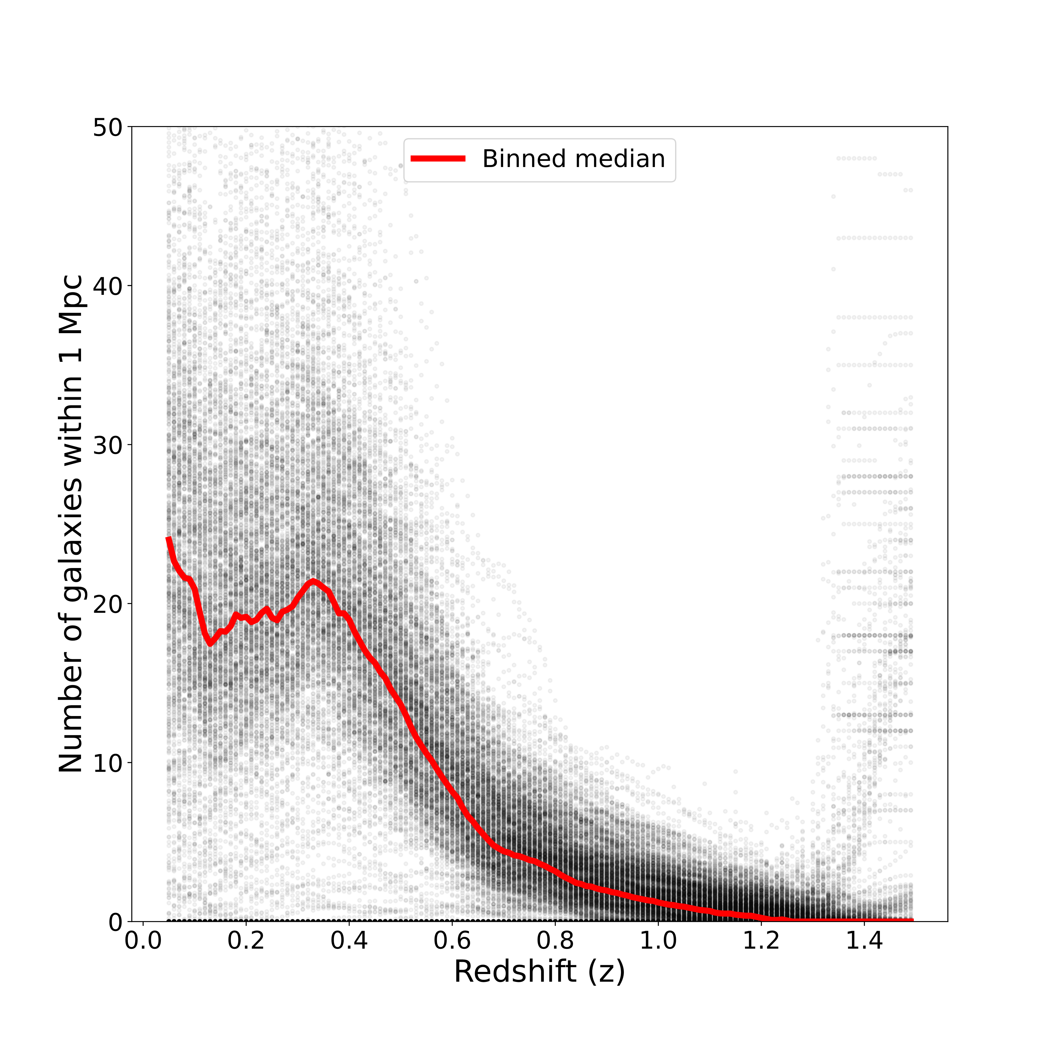
Figure 13: Number of galaxies within 1 Mpc at random sky pointings vs photometric redshift. The rise in galaxies above $z$=1.2 is likely caused by misclassified stars, but they do not affect the median which remains at 0. The data in this graph are for the South (DECaLS) portion of the DESI Legacy Survey; the exact same process was applied for the North (BASS/MzLS) portion and yielded similar results. A comparison between the resulting median backgrounds for North and South are shown in Figure 15.

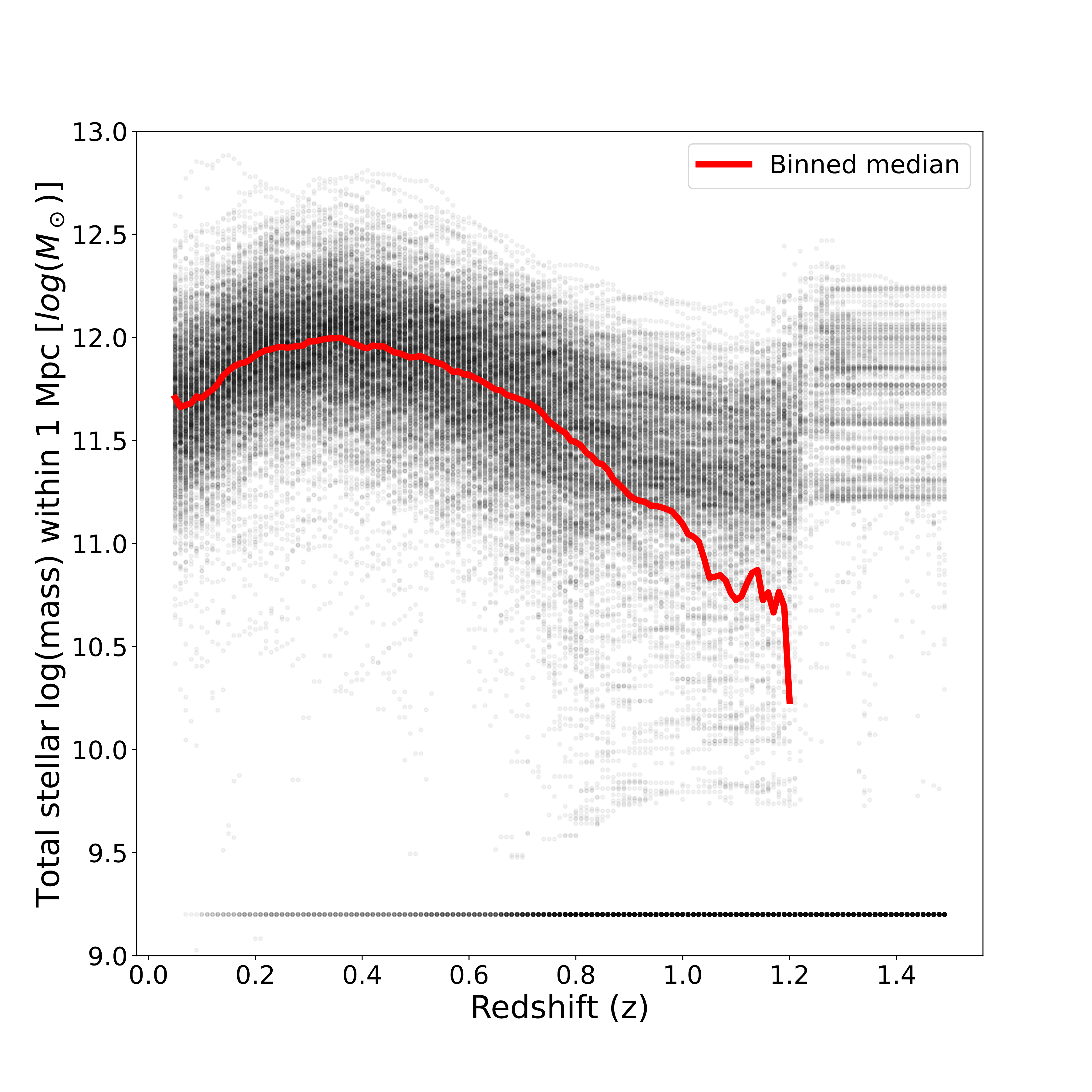
Figure 14: 1-Mpc total stellar log(mass) at random sky pointings vs photometric redshift. Pointings which do not contain any galaxies (stellar mass = 0) are plotted at log(mass) = 9.2. For galaxies at $z$>1.2, stellar masses become unreliable. The data in this graph are for the North (BASS/MzLS) portion of the DESI Legacy Survey; the exact same process was applied for the South (DECaLS) portion and yielded similar results. A comparison between the resulting median backgrounds for North and South are shown in Figure 16.

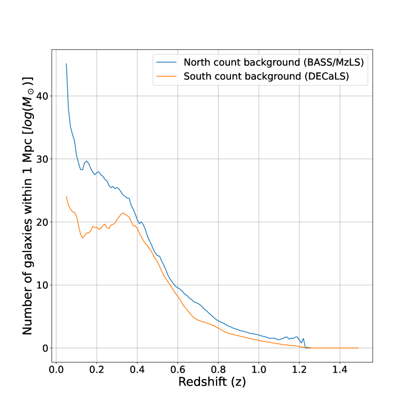
Figure 15: Median background galaxy counts within 1 Mpc vs photometric redshift. The differences in backgrounds between North and South are due to differing survey characteristics and different models for redshift for each survey.

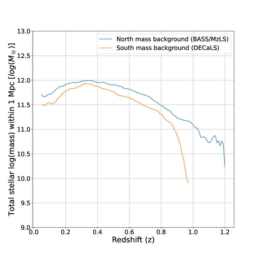
Figure 16: Median background 1-Mpc total stellar log(mass) vs photometric redshift. For galaxies at $z$>1.2, stellar masses become unreliable. The differences in mass backgrounds between North and South are due to differing survey characteristics and different models for stellar mass and redshift for each survey.

Appendix B Stellar Mass Incompleteness Correction

The galaxy sample used by our algorithm is magnitude-limited (see 2). Low-stellar-mass galaxies are thus excluded from our catalogue at a rate which increases with redshift. Thus, in order to obtain a redshift-independent total stellar mass estimate for each cluster, we must correct for the stellar mass incompleteness of our data. To correct for stellar mass incompleteness, we apply a redshift-dependent scaling factor to the galaxy cluster stellar masses. This factor is determined by creating a stellar mass model based on the Schechter function (Schechter, 1976):

$$\Phi(M)dM=\Phi^{\star}\left(\frac{M}{M_{\star}}\right)^{\alpha}exp\left(\frac{-M}{M_{\star}}\right)\frac{dM}{M_{\star}},$$ (7)

where $M$ is the galaxy stellar mass, $M_{\star}$ is the characteristic galaxy stellar mass where the power-law form of the function ends, $\Phi(M)$ is the number density of galaxies with a mass $M$, and $\Phi_{\star}$ is the normalization factor. We fit this model to the high-mass end of the mass distribution histograms of galaxies observed to be in a cluster. We are able to use this method since we observe the histograms at all redshifts to roughly follow the Schechter function at high masses, though the number count approaches 0 for low mass galaxies (an example of a stellar mass histogram is shown in Figure 18).

As the first step of building our model, we use the Schechter function to approximate the true mass distribution of galaxies, given by the double Schechter function (Davidzon et al., 2017)

$$\Phi(M)dM=\left(\Phi_{1}^{\star}\left(\frac{M}{M_{\star}}\right)^{\alpha_{1}}+\Phi_{2}^{\star}\left(\frac{M}{M_{\star}}\right)^{\alpha_{2}}\right)exp\left(\frac{-M}{M_{\star}}\right)\frac{dM}{M_{\star}}$$ (8)

. This approximation is necessary in order to reduce the number of parameters to be fitted. A demonstration of the sufficiency of a single Schechter function to fit to a double Schechter function above $log(M)=10$ is shown in Figure 17. We fit $\alpha$ in our model to the double Schechter for the values shown in Table 1. $M_{\star}$ and $\Phi(M)$ in our model are fitted to the stellar mass distribution of galaxies in our clusters.

We fit $M_{\star}$ and $\Phi^{\star}$ to the high-mass end of the galaxy mass distribution histogram for several redshift bins (as an example, see Figure 18). We use 22 redshift bins between 0.025<$z$<1.025 with bin width $z$=0.05. The high-mass ends of each histogram are located by fitting a piecewise linear function of the form

$$Limit\hskip 2.84526ptlog(M_{\odot})=minimum(a*z+b,11.2)$$ (9)

to the peaks of the histograms, where z is redshift bin. The maximum limit of $log(M_{odot})=11.2$ is required in order to ensure that the mass of the cluster central galaxy is not excluded from the mass calculation in the main algorithm (see section 3.2). We find the best-fit values to be a = 1.36202 and b = 9.96855. This model, along with an example of actual histogram peak locations for a small sample of galaxies, is shown in Figure 19.

The contribution of missing low-mass galaxies to the total stellar mass is determined by taking the ratio between the integral of Equation 7 from $log(M)=10$ to infinity and the integral of Equation 7 from the mass limit 9 to infinity. The latter integral represents the incomplete stellar mass calculated by the main algorithm. The ratio between the integrals is thus

$$factor=M_{tot}/M{inc},$$ (10)

where $M_{tot}$ is the total stellar mass above $log(M)=10$ and $M{inc}$ is the incomplete (observed) stellar mass. Multiplying the observed galaxy cluster stellar masses by this redshift-dependent mass correction factor allows us to estimate the true stellar masses above $log(M)=10$ within the 1 Mpc, 0.5 Mpc, and 0.1 Mpc search radii. We find that a quadratic equation is a good fit for the observed log(stellar mass) correction factor as a function of redshift:

$$log(factor(z))=az^{2}+bz+c,$$ (11)

where a = 0.19347, b = 0.23392, and c = 0.00694. A plot of the stellar mass correction factor as a function of redshift is shown in Figure 20; we trained this model on a dataset consisting of 150 sweep files randomly chosen from DESI Legacy Survey North and South. The stellar mass correction factor is provided for all galaxy clusters in our catalogue so that the incomplete stellar mass can be easily retrieved.

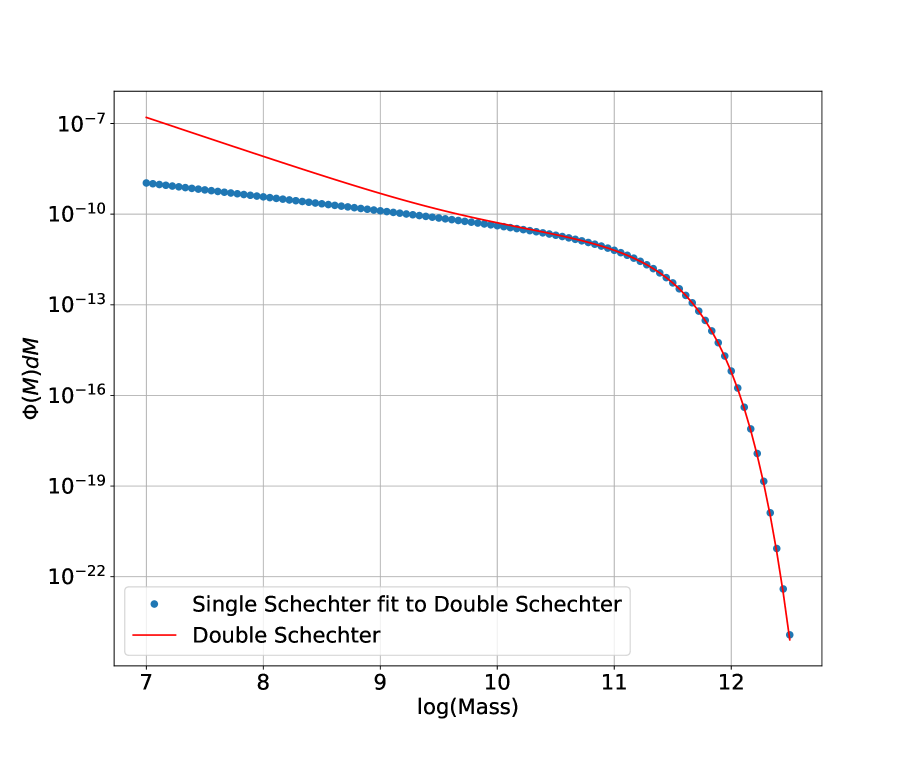
Figure 17: Comparison of the Double Schechter function with the best-fit Schechter function as an approximation. The best-fit Schechter is a very good approximation to the high-mass end of the Double Schechter function, down to approximately $log(M_{\odot})=10$. The parameters for the Double Schechter in this example are $\Phi_{1}^{\star}=0.098,\hskip 5.69054pt\alpha_{1}=-1.3,\hskip 5.69054pt\Phi_{2}^{\star}=1.58,\hskip 5.69054pt\alpha_{2}=-0.39,\hskip 5.69054ptlog(M_{\star})=10.83$. The parameters for the best-fit Schechter function are $\Phi^{\star}=1.663,\hskip 5.69054pt\alpha=-0.459,\hskip 5.69054ptlog(M_{\star})=11.043$. Assuming different parameters for the Double Schechter function results in similarly well-fitting Schechter approximations.

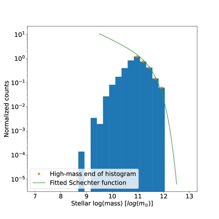
Figure 18: An example of fitting a Schechter function to the observed galaxy stellar mass histogram for the redshift bin centered on z = 0.66. The histogram follows a Schechter function above log(mass) = 11, but below this mass the number counts decrease due to incompleteness. The Stellar Mass Correction Factor (Equation 10) is the ratio between two integrals along the green line (Schechter function): the total mass is the integral above log(mass) = 10, and the incomplete mass is the integral above the peak of the histogram (in this case, above log(mass) = 11). This ratio is designed to compensate for the missing galaxy counts for galaxies with masses below log(mass) = 11.

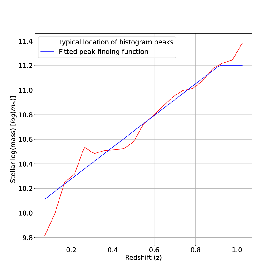
Figure 19: The histogram peak-finding function used to determine the log(mass) above which stellar mass histograms should roughly follow a Schechter function. The red line is the location of histogram peaks for one example sweep; there is good correspondence between the model and the example. In practice, we use many sweeps simultaneously when training the Stellar Mass Correction Factor (Equation 10), which reduces the random variation in histogram peak location.

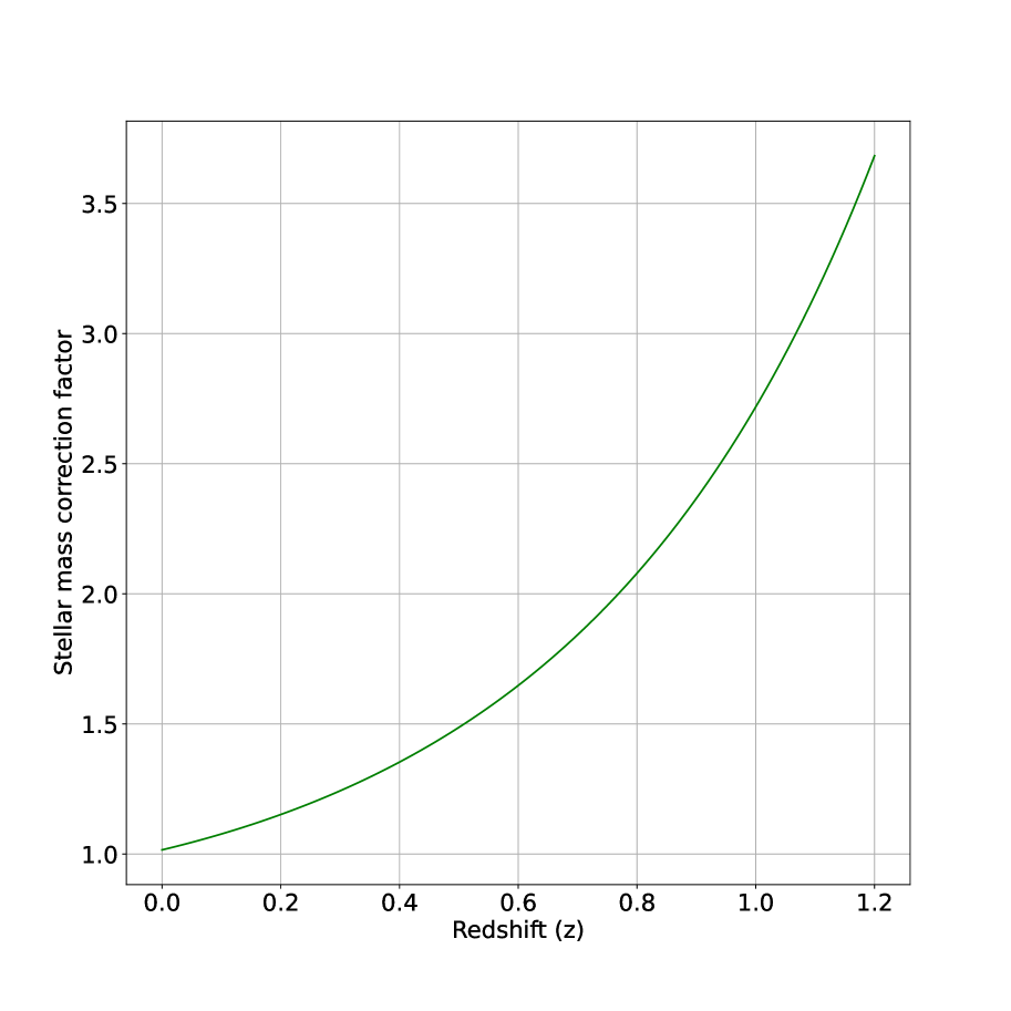
Figure 20: Stellar Mass Correction Factor (Equation 10) as a function of redshift. Mass incompleteness increases with redshift (higher mass limit), so the correction factor increases correspondingly.

Table 1: Schechter parameters used to derive Stellar Mass Correction Factor

Double Schechter Parameters
$Redshift$	$log(M_{\odot})$	$\alpha_{1}$	$\Phi_{1}(e5)$	$\alpha_{2}$	$\Phi_{2}(e5)$
$0.1<z<0.5$	$10.97$	$-0.75$	$79.53$	$-2.04$	$0.18$
$0.5<z<0.8$	$10.90$	$-0.50$	$92.06$	$-2.14$	$0.09$
$0.8<z<1.1$	$10.87$	$-0.44$	$102.63$	$-2.14$	$0.07$
Best-fit Schechter Parameters
$Redshift$	$M_{\odot}$	$\alpha$	$\Phi$
$0.1<z<0.5$	varies with $z$	$-0.7535$	varies with $z$
$0.5<z<0.8$	varies with $z$	$-0.5015$	varies with $z$
$0.8<z<1.1$	varies with $z$	$-0.441$	varies with $z$

Appendix C Gravitationally Lensed Quasar Candidates

As a supplement to our galaxy cluster catalogue and galaxy cluster member catalogue, we provide a catalogue of candidate gravitationally lensed quasars. Gravitationally lensed quasars are valuable as probes of the Hubble parameter for the expansion of the universe (Suyu et al., 2017). As data, we used quasars from the DESI Bright and Dark survey target selection (Myers et al., 2023). We compiled the candidate lensed quasar catalogue by counting the number of quasars within the Einstein radius of each galaxy cluster identified by CluMPR. We use two Einstein radii: one corresponds to wide angle lensing by the entire cluster ($M=10^{15}M_{\odot}$), and the other corresponds to lensing by the core of the cluster ($M=0.25*10^{15}M_{\odot}$). Since there is contamination of QSO targets by stars, particularly in dense star fields, we remove galaxy clusters which have counts within 3 Einstein radii >= 6 times the counts within one Einstein radius. We rate candidates based on how many of the quasars have similar colors in bands g-r, g-z, and r-W1. If at least two quasars are within 1 magnitude of each other in all 3 colors, we rate the candidate at Grade C. If at least three quasars are within 1 magnitude of each other in all 3 colors, we rate the the candidate at Grade B. If either 4 quasars or two combinations of 3 quasars are within 1 magnitude of each other in all 3 colors, we rate the candidate as Grade A. Spectroscopic follow-up of the lensed quasar candidates and cluster lens modeling will enable confirmation of true lensed quasars.

C.1 Recovery of known cluster-lensed quasars

To date, six widely-separated gravitationally lensed quasars (corresponding to a cluster-scale lens mass) have been discovered (Inada et al., 2003, 2006; Dahle et al., 2013; Shu et al., 2018, 2019; Martinez et al., 2023). Of the six known cluster-lensed quasars, we recover three: SDSS J1004+4112 (Grade A core-lensed), SDSS J1029+2623 (Grade C core-lensed), and COOL J0542-2125 (Grade A core-lensed). We do not recover SDSSJ2222+2745 or SDSS J1326+4806 due to only one of the quasar images being in the DESI target catalogues as a QSO, and we do not recover SDSS J0909+4449 due to the lensing cluster being absent from both the CluMPR and Zou et al. (2021) catalogues (it is more accurately described as a galaxy group).

C.2 New Grade A core-lensed candidates

Of the five core-lensed candidates ranked Grade A, two are known lensed quasars. We discuss the remaining Grade A core-lensed candidates below.

C.2.1 CluMPR J1278885160133433856: A candidate lensed changing-look quasar

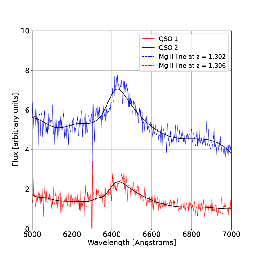
Figure 24: Close-up of the MgII broad emission line. QSO 1 has an SDSS redshift estimate of 1.306, while QSO 2 has an SDSS redshift estimate of 1.302. The black lines are cubic spline fits to the spectra.

The candidate lensed quasars located near the cluster CluMPR J1278885160133433856 are shown in Figure 21. The galaxy cluster has an SDSS spectroscopic redshift of $z$=0.525, and the cluster center galaxy is located at RA = 127.8885, DEC = 43.4339 (J2000). Two of the candidate lensed images, QSO 1 and QSO 2, are confirmed quasars with SDSS redshifts of $z=1.3056\pm 0.0002$ and $z=1.3021\pm 0.0004$, respectively. The spectra of these quasars are shown in Figure 22, with zoomed-in views of the C III] and Mg II broad emission lines (Figures 23 and 24, respectively). The alignment between emission lines in the two spectra indicates that QSO 1 and QSO 2 are at the same or nearly the same redshift ($z\approx 1.3$), but the noise in the spectra and the absence of narrow emisison lines makes evaluating the accuracy of the assigned SDSS spectroscopic redshifts challenging. There are notable differences between the spectra: QSO 2 appears brighter and has a redder color (negative slope) compared to QSO 1, and the broad emission lines appear more prominent in QSO 2 than in QSO 1.

We offer two potential explanations for the differences in the spectra: either these are two distinct quasars that happen to be at very similar redshifts, or these are two images of the same highly-variable ("changing-look") quasar. Changing-look quasars are quasars whose luminosity and colors (i.e., continuum slopes) change quickly by a large factor over the course of hundreds of days to several years (e.g. Bian et al., 2012; MacLeod et al., 2016, 2019). The luminosity changes are accompanied by the appearance and disappearance of broad emission lines (e.g. LaMassa et al., 2015; Runnoe et al., 2016; Ruan et al., 2016). Changing-look quasars have recently been discovered at redshifts beyond 1 (Ross et al., 2020; Guo et al., 2020). The variability timescale of changing look quasars is on the same order as the time delays between lensed images for a cluster-scale lens, so it is possible that the difference in spectra between QSO 1 and QSO 2 is due to a gravitational time delay.

To evaluate the changing look quasar interpretation further, we consider the following:

• According to the formal uncertainties, the redshifts of the two quasars ($\sim 30$–$50~{}{\rm km~{}s}^{-1}$) differ by $\approx 8\sigma$. However, the detailed discussion of redshift determination methods used by the SDSS by Lyke et al. (2020, see their Section 4.6 and Figure A1) suggests a much larger redshift uncertainty of $\sim 300~{}{\rm km~{}s}^{-1}$. Viewed in this light, the quasar redshifts differ only by $1.5\sigma$.

• We measured the rest-frame equivalent widths of the broad emission lines and found them to be ${\rm EW(Mg\;II)}=34\pm 2$ Å and ${\rm EW(C\;III])}=33\pm 3$ Å in QSO 1 and ${\rm EW(Mg\;II)}=26\pm 1$ Å and ${\rm EW(C\;III])}=25\pm 1$ Å in QSO 2. These measurements reflect the Baldwin effect (anti-correlation between EW and luminosity; e.g., Green et al., 2001, and references therein) and follow the behavior seen in extremely variable quasars by Ren et al. (2022).

• A caveat to the above is that, the relative luminosities of the two quasars cannot be readily evaluated as the observed brightness of quasar images depends on the magnification of the lens (Bauer et al., 2011), so the true luminosity of the quasar images cannot be estimated without a well-constrained mass model for the lens.

The above considerations suggest that the the lensed changing-look quasar hypothesis remains plausible for QSO 1 and QSO 2. To test this hypothesis further we suggest the following.

• Improving the redshift determination. – This can be done by obtaining spectra with higher signal-to-noise ratio in the near-IR or sub-mm bands to detect narrow emission lines. Spectra in the wavelength range 7800–8600 Å can catch the narrow [Ne V] $\lambda\lambda$3346,3426 and [O II] $\lambda\lambda$3726,3729 doublets. The wavelengths of these lines and their relative strengths (the [Ne V]/[O II] ratio) can test the hypothesis that QSO 1 and QSO 2 are lensed images of the same quasar. In the same spirit, spectroscopy in the J band can catch the H$\beta$ line and [O III] $\lambda\lambda$4959,5007 doublet and allow a similar test. Alternatively, spectroscopy with ALMA may detect the CO(2-1) line from the quasar host galaxies (rest frequency of 230.5 GHz) that will allow for an exquisite redshift determination.

• Monitoring for spectroscopic variability. – If the spectra of QSO 1 and QSO 2 do indeed reflect a change in the state of a single quasar, we should expect that one of the two spectra will change to match the other in the next few years. Therefore, the hypothesis can be tested by repeated spectroscopic observations of the two quasars.

There are two more possible quasar images (C1 and C2) which have been selected for DESI spectroscopy. Finally, there is a dim object resembling a lensing arc. Further spectroscopy and deeper imaging are necessary to determine whether these objects are related to QSO 1 and QSO 2.

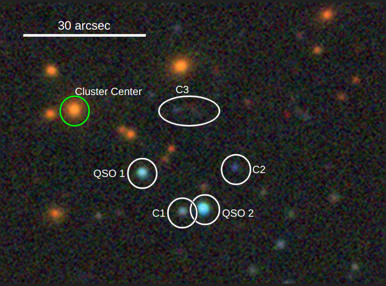
Figure 21: Candidate gravitationally lensed quasar system near galaxy cluster CluMPR J1278885160133433856 (cluster center galaxy in green). QSO 1 and QSO 2 are confirmed quasars with SDSS redshifts of 1.306 and 1.302, respectively. Objects C1 and C2 are QSO targets for DESI. C3 is a very faint object which resembles a lensing arc.

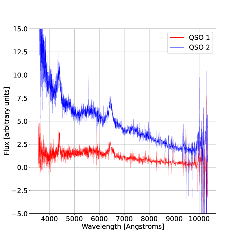
Figure 22: SDSS spectra for QSO 1 and QSO 2 in the candidate gravitationally lensed quasar system near galaxy cluster CluMPR J1278885160133433856. The broad emission lines (CIII] and MgII) are redshifted to very similar values near $z=1.3$, but the slopes of the spectra are very different. This indicates that these are either two different quasars located at the same redshift, or two images of the same highly variable (changing-look) quasar.

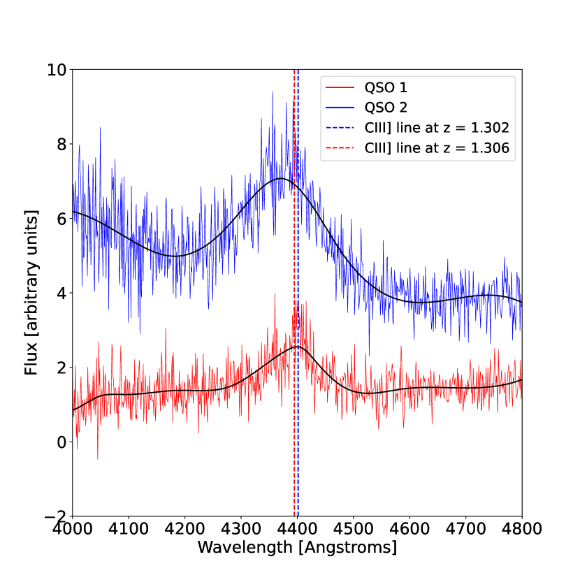
Figure 23: Close-up of the CIII] broad emission line. QSO 1 has an SDSS redshift estimate of 1.306, while QSO 2 has an SDSS redshift estimate of 1.302. The spectrum for QSO 2 has been shifted down by a constant of 3 flux units in order to improve legibility. The black lines are cubic spline fits to the spectra.

C.2.2 CluMPR J2439482900096790528

The candidate lensed quasars located near the cluster CluMPR J2439482900096790528 are shown in Figure 25. The galaxy cluster’s central galaxy is located at the photometric redshift $z=0.333$ with RA = 243.9483, DEC = 6.7904. There are no publicly available spectra for the candidate quasars at this time, but they are part of the DESI dark time targets. Spectroscopy and deeper imaging are necessary to determine whether this system is a quasar-lensing cluster.

Figure 25: Candidate gravitationally lensed quasar system near galaxy cluster CluMPR J2439482900096790528 (cluster center galaxy in green). Objects in white circles are QSO targets for DESI, and there is a possibility that they are all images of the same gravitationally lensed quasar.

C.2.3 CluMPR J2420498300113853952

The candidate lensed quasars located near the cluster CluMPR J2420498300113853952 are shown in Figure 26. The galaxy cluster’s central galaxy is located at the photometric redshift $z=0.750$ with RA = 242.0498, DEC = 23.8542. One of the candidate quasars (QSO 1) has SDSS spectroscopy with a spectroscopic redshift of 2.205. There are no publicly available spectra for the other candidate quasars at this time, but they are part of the DESI dark time targets. Spectroscopy and deeper imaging are necessary to determine whether this system is a quasar-lensing cluster.

Figure 26: Candidate gravitationally lensed quasar system near galaxy cluster CluMPR J2420498300113853952 (cluster center galaxy in green). Objects in white circles are QSO targets for DESI, and there is a possibility that some of them are images of the same gravitationally lensed quasar (it is relatively unlikely that they are all the same quasar due to their configuration). QSO 1 is a confirmed quasar with SDSS spectroscopic redshift of 2.205.

Appendix D catalogue descriptions

Below we provide descriptions of the column names and contents for the CluMPR DESI Legacy Survey catalogue, associated cluster member catalogue, and the candidate gravitationally lensed quasar catalogues. The public location of the catalogues can be found in the Data Availability) section.

Table 2: Main CluMPR Galaxy Cluster catalogue

Columns	Description
Index	Sequential number in catalogue
RA_central	Right ascension of central cluster galaxy (deg)
DEC_central	Declination of central cluster galaxy (deg)
z_spec	Spectroscopic redshift of central cluster galaxy (-1 if unavailable)
z_spec_err	Estimated error in spectroscopic redshift of central cluster galaxy (-1 if unavailable)
z_median_central	Median photometric redshift of central cluster galaxy
z_average_no_wt	Mean photometric redshift of all cluster galaxies
z_average_prob	Mean photometric redshift of all cluster galaxies, weighted by membership probability
z_average_mass_prob	Mean photometric redshift of all cluster galaxies, weighted by membership probability times mass
z_std_central	Std. deviation of photometric redshift of central cluster galaxy
z_std_no_wt	Std. deviation of photometric redshift of all cluster galaxies
z_std_prob	Std. deviation of photometric redshift of all cluster galaxies, weighted by membership probability
z_std_mass_prob	Std. deviation of photometric redshift of all cluster galaxies, weighted by membership probability times mass
gid	Unique identifier of the central cluster galaxy. See Section 3.2 for definition.
mass_central	Log(stellar mass) of the central cluster galaxy
cluster_mass_onempc	Log(stellar mass) of the cluster within a 1-Mpc physical radius, corrected for incompleteness and galaxy background
cluster_mass_halfmpc	Log(stellar mass) of the cluster within a 0.5-Mpc physical radius, corrected for incompleteness and galaxy background
cluster_mass_tenthmpc	Log(stellar mass) of the cluster within a 0.1-Mpc physical radius, corrected for incompleteness and galaxy background
richness_onempc	Expectation number of observed galaxies in cluster within a 1-Mpc physical radius, corrected for galaxy background
richness_halfmpc	Expectation number of observed galaxies in cluster within 0.5-Mpc physical radius, corrected for galaxy background
richness_tenthmpc	Expectation number of observed galaxies in cluster within 0.1-Mpc physical radius, corrected for galaxy background

Table 3: Extended CluMPR Galaxy Cluster catalogue

Columns	Description
Index	Sequential number in catalogue
RA_central	Right ascension of central cluster galaxy (deg)
DEC_central	Declination of central cluster galaxy (deg)
z_spec	Spectroscopic redshift of central cluster galaxy (-1 if unavailable)
z_spec_err	Estimated error in spectroscopic redshift of central cluster galaxy (-1 if unavailable)
z_median_central	Median photometric redshift of central cluster galaxy
z_average_no_wt	Mean photometric redshift of all cluster galaxies
z_average_prob	Mean photometric redshift of all cluster galaxies, weighted by membership probability
z_average_mass_prob	Mean photometric redshift of all cluster galaxies, weighted by membership probability times mass
z_std_central	Std. deviation of photometric redshift of central cluster galaxy
z_std_no_wt	Std. deviation of photometric redshift of all cluster galaxies
z_std_prob	Std. deviation of photometric redshift of all cluster galaxies, weighted by membership probability
z_std_mass_prob	Std. deviation of photometric redshift of all cluster galaxies, weighted by membership probability times mass
RELEASE	Integer denoting the camera and filter set used for the central galaxy, which will be unique for a given processing run of the data,
	from Tractor catalogues
BRICKID	A unique Brick ID for the central galaxy, from Tractor catalogues
OBJID	catalogue object number within this brick for the central galaxy, from Tractor catalogues
MASKBITS	Bitwise mask indicating that the central galaxy touches a pixel in the coadd/*/*/*maskbits* maps, from Tractor catalogues
gid	Unique identifier of the central cluster galaxy. See Section 3.2 for definition.
mass_central	Log(stellar mass) of the central cluster galaxy
cluster_mass_onempc	Log(stellar mass) of the cluster within a 1-Mpc physical radius, corrected for incompleteness and galaxy background
cluster_mass_halfmpc	Log(stellar mass) of the cluster within a 0.5-Mpc physical radius, corrected for incompleteness and galaxy background
cluster_mass_tenthmpc	Log(stellar mass) of the cluster within a 0.1-Mpc physical radius, corrected for incompleteness and galaxy background
mass_bkgd_onempc	Mass background (which has been subtracted from cluster_mass_onempc) for one-mpc radius
mass_bkgd_halfmpc	Mass background (which has been subtracted from cluster_mass_onempc) for one-mpc radius
mass_bkgd_tenthmpc	Mass background (which has been subtracted from cluster_mass_onempc) for one-mpc radius
correction_factor	Correction factor for mass incompleteness
neighbours_onempc	Expectation number of observed galaxies in cluster within a 1-Mpc physical radius, not corrected for galaxy background
neighbours_halfmpc	Expectation number of observed galaxies in cluster within a 0.5-Mpc physical radius, not corrected for galaxy background
neighbours_tenthmpc	Expectation number of observed galaxies in cluster within a 0.1-Mpc physical radius, not corrected for galaxy background
richness_onempc	Expectation number of observed galaxies in cluster within a 1-Mpc physical radius, corrected for galaxy background
richness_halfmpc	Expectation number of observed galaxies in cluster within 0.5-Mpc physical radius, corrected for galaxy background
richness_tenthmpc	Expectation number of observed galaxies in cluster within 0.1-Mpc physical radius, corrected for galaxy background
flag_foreground	1 indicates the presence of a major foreground galaxy (cluster parameters may be unreliable in such cases).
	Value 0 should indicate good clusters.
edge_mask	0 indicates that the cluster is located close enough to the edge of the footprint that parameters may be affected.
	Value 1 should indicate good clusters.
flag_footprint	1 indicates a galaxy cluster which is located in an isolated area of the footprint (these are excluded from the main dataset).

Table 4: CluMPR Galaxy Cluster Membership catalogue

Columns	Description
Galaxy	Unique galaxy id, constructed as gid above. See Section 3.2 for definition
Cluster	Unique galaxy id of cluster central galaxy
Galaxy Mass	Stellar mass of galaxy
Galaxy Redshift	Photometric redshift of galaxy
Cluster Redshift	Median photometric redshift of cluster central galaxy
Galaxy Redshift Uncertainty	Uncertainty in the photometric redshift of this galaxy
Cluster Membership Probability	Cluster membership probability of this galaxy

Table 5: Candidate Lensed Quasar catalogues

Columns	Description
lens_RA_central	Right ascension of central cluster galaxy (deg)
lens_DEC_central	Declination of central cluster galaxy (deg)
lens_z_spec	Spectroscopic redshift of central cluster galaxy (-1 if unavailable)
lens_z_spec_err	Estimated error in spectroscopic redshift of central cluster galaxy (-1 if unavailable)
lens_z_median_central	Median photometric redshift of central cluster galaxy
cluster_mass_onempc	Log(stellar mass) of the cluster within a 1-Mpc physical radius, corrected for incompleteness and galaxy background
lens_gid	Unique identifier of the central cluster galaxy. See Section 3.2 for definition.
QSO_RA	Right ascension of each QSO (deg)
QSO_DEC	Declination of each QSO (deg)
g_r	g-r color of each QSO
g_z	g-z color of each QSO
r_w1	r-w1 color of each QSO

References

- Aihara et al. (2011) Aihara H., et al., 2011, ApJS, 193, 29
- Aihara et al. (2018) Aihara H., et al., 2018, PASJ, 70, S4
- Barton et al. (2007) Barton E. J., Arnold J. A., Zentner A. R., Bullock J. S., Wechsler R. H., 2007, ApJ, 671, 1538
- Bauer et al. (2011) Bauer A. H., Seitz S., Jerke J., Scalzo R., Rabinowitz D., Ellman N., Baltay C., 2011, ApJ, 732, 64
- Bayliss et al. (2014) Bayliss M. B., Rigby J. R., Sharon K., Wuyts E., Florian M., Gladders M. D., Johnson T., Oguri M., 2014, ApJ, 790, 144
- Bennett et al. (2014) Bennett C. L., Larson D., Weiland J. L., Hinshaw G., 2014, ApJ, 794, 135
- Berrier et al. (2011) Berrier H. D., Barton E. J., Berrier J. C., Bullock J. S., Zentner A. R., Wechsler R. H., 2011, ApJ, 726, 1
- Bezanson et al. (2022) Bezanson R., et al., 2022, arXiv e-prints, p. arXiv:2212.04026
- Bian et al. (2012) Bian W.-H., Zhang L., Green R., Hu C., 2012, ApJ, 759, 88
- Blanton et al. (2006) Blanton M. R., Eisenstein D., Hogg D. W., Zehavi I., 2006, ApJ, 645, 977
- Blanton et al. (2017) Blanton M. R., et al., 2017, AJ, 154, 28
- Cornachione et al. (2018) Cornachione M. A., et al., 2018, ApJ, 853, 148
- DESI Collaboration et al. (2022) DESI Collaboration et al., 2022, AJ, 164, 207
- Dahle et al. (2013) Dahle H., et al., 2013, ApJ, 773, 146
- Dark Energy Survey Collaboration et al. (2016) Dark Energy Survey Collaboration et al., 2016, MNRAS, 460, 1270
- Davidzon et al. (2017) Davidzon I., et al., 2017, A&A, 605, A70
- Dey et al. (2019) Dey A., et al., 2019, AJ, 157, 168
- Dressler (1980) Dressler A., 1980, ApJ, 236, 351
- Euclid Collaboration et al. (2022) Euclid Collaboration et al., 2022, A&A, 662, A112
- Flaugher et al. (2015) Flaugher B., et al., 2015, AJ, 150, 150
- Freeman et al. (2009) Freeman P. E., Newman J. A., Lee A. B., Richards J. W., Schafer C. M., 2009, MNRAS, 398, 2012
- Goobar et al. (2017) Goobar A., et al., 2017, Science, 356, 291
- Goobar et al. (2023) Goobar A., et al., 2023, Nature Astronomy
- Green et al. (2001) Green P. J., Forster K., Kuraszkiewicz J., 2001, ApJ, 556, 727
- Guo et al. (2020) Guo H., et al., 2020, ApJ, 905, 52
- Haiman et al. (2001) Haiman Z., Mohr J. J., Holder G. P., 2001, ApJ, 553, 545
- Hogg et al. (2004) Hogg D. W., et al., 2004, ApJ, 601, L29
- Inada et al. (2003) Inada N., et al., 2003, Nature, 426, 810
- Inada et al. (2006) Inada N., et al., 2006, ApJ, 653, L97
- Ivison et al. (2020) Ivison R. J., Richard J., Biggs A. D., Zwaan M. A., Falgarone E., Arumugam V., van der Werf P. P., Rujopakarn W., 2020, MNRAS, 495, L1
- Johnson et al. (2017) Johnson T. L., et al., 2017, ApJ, 843, L21
- Kauffmann et al. (2004) Kauffmann G., White S. D. M., Heckman T. M., Ménard B., Brinchmann J., Charlot S., Tremonti C., Brinkmann J., 2004, MNRAS, 353, 713
- Kelly et al. (2015) Kelly P. L., et al., 2015, Science, 347, 1123
- Khullar et al. (2021) Khullar G., et al., 2021, ApJ, 906, 107
- LSST Science Collaboration et al. (2009) LSST Science Collaboration et al., 2009, arXiv e-prints, p. arXiv:0912.0201
- LaMassa et al. (2015) LaMassa S. M., et al., 2015, ApJ, 800, 144
- Livermore et al. (2015) Livermore R. C., et al., 2015, MNRAS, 450, 1812
- Lyke et al. (2020) Lyke B. W., et al., 2020, ApJS, 250, 8
- MacLeod et al. (2016) MacLeod C. L., et al., 2016, MNRAS, 457, 389
- MacLeod et al. (2019) MacLeod C. L., et al., 2019, ApJ, 874, 8
- Martinez et al. (2023) Martinez M. N., et al., 2023, ApJ, 946, 63
- Meyers et al. (2009) Meyers J., et al., 2009, in American Astronomical Society Meeting Abstracts #213. p. 481.05
- Moustakas et al. (2021) Moustakas J., et al., 2021, in American Astronomical Society Meeting Abstracts. p. 527.04
- Myers et al. (2023) Myers A. D., et al., 2023, AJ, 165, 50
- Napier et al. (2023) Napier K., Sharon K., Dahle H., Bayliss M., Gladders M. D., Mahler G., Rigby J. R., Florian M., 2023, arXiv e-prints, p. arXiv:2301.11240
- Newman et al. (2002) Newman J. A., Marinoni C., Coil A. L., Davis M., 2002, PASP, 114, 29
- Refsdal (1964) Refsdal S., 1964, MNRAS, 128, 307
- Ren et al. (2022) Ren W., Wang J., Cai Z., Guo H., 2022, ApJ, 925, 50
- Rivera-Thorsen et al. (2019) Rivera-Thorsen T. E., et al., 2019, Science, 366, 738
- Rodriguez & Laio (2014) Rodriguez A., Laio A., 2014, Science, 344, 1492
- Ross et al. (2020) Ross N. P., Graham M. J., Calderone G., Ford K. E. S., McKernan B., Stern D., 2020, MNRAS, 498, 2339
- Ruan et al. (2016) Ruan J. J., et al., 2016, ApJ, 826, 188
- Runnoe et al. (2016) Runnoe J. C., et al., 2016, MNRAS, 455, 1691
- Rykoff et al. (2014) Rykoff E. S., et al., 2014, ApJ, 785, 104
- Rykoff et al. (2016) Rykoff E. S., et al., 2016, ApJS, 224, 1
- Schechter (1976) Schechter P., 1976, ApJ, 203, 297
- Shu et al. (2018) Shu Y., Marques-Chaves R., Evans N. W., Pérez-Fournon I., 2018, MNRAS, 481, L136
- Shu et al. (2019) Shu Y., Koposov S. E., Evans N. W., Belokurov V., McMahon R. G., Auger M. W., Lemon C. A., 2019, MNRAS, 489, 4741
- Silva et al. (2016) Silva D. R., et al., 2016, in American Astronomical Society Meeting Abstracts #228. p. 317.02
- Simet et al. (2017) Simet M., McClintock T., Mandelbaum R., Rozo E., Rykoff E., Sheldon E., Wechsler R. H., 2017, MNRAS, 466, 3103
- Spergel et al. (2015) Spergel D., et al., 2015, arXiv e-prints, p. arXiv:1503.03757
- Suyu et al. (2017) Suyu S. H., et al., 2017, MNRAS, 468, 2590
- The Dark Energy Survey Collaboration (2005) The Dark Energy Survey Collaboration 2005, arXiv e-prints, pp astro–ph/0510346
- Virtanen et al. (2020) Virtanen P., et al., 2020, Nature Methods, 17, 261
- Wen & Han (2015) Wen Z. L., Han J. L., 2015, ApJ, 807, 178
- Wen & Han (2021) Wen Z. L., Han J. L., 2021, MNRAS, 500, 1003
- Wen & Han (2022) Wen Z. L., Han J. L., 2022, MNRAS, 513, 3946
- Wen et al. (2009) Wen Z. L., Han J. L., Liu F. S., 2009, ApJS, 183, 197
- Wen et al. (2012) Wen Z. L., Han J. L., Liu F. S., 2012, ApJS, 199, 34
- Wittman et al. (2023) Wittman D., Stancioli R., Finner K., Bouhrik F., van Weeren R., Botteon A., 2023, arXiv e-prints, p. arXiv:2306.01715
- Wong et al. (2020) Wong K. C., et al., 2020, MNRAS, 498, 1420
- Wright et al. (2010) Wright E. L., et al., 2010, AJ, 140, 1868
- Yang et al. (2021) Yang X., et al., 2021, ApJ, 909, 143
- Zhou et al. (2021) Zhou R., et al., 2021, MNRAS, 501, 3309
- Zhou et al. (2023) Zhou R., et al., 2023, AJ, 165, 58
- Zou et al. (2017) Zou H., et al., 2017, PASP, 129, 064101
- Zou et al. (2021) Zou H., et al., 2021, ApJS, 253, 56