Refining the Stellar Parameters of $\tau$ Ceti: a Pole-on Solar Analog

Abstract

To accurately characterize the planets a star may be hosting, stellar parameters must first be well-determined. $\tau$ Ceti is a nearby solar analog and often a target for exoplanet searches. Uncertainties in the observed rotational velocities have made constraining $\tau$ Ceti’s inclination difficult. For planet candidates from radial velocity (RV) observations, this leads to substantial uncertainties in the planetary masses, as only the minimum mass ($m\sin i$) can be constrained with RV. In this paper, we used new long-baseline optical interferometric data from the CHARA Array with the MIRC-X beam combiner and extreme precision spectroscopic data from the Lowell Discovery Telescope with EXPRES to improve constraints on the stellar parameters of $\tau$ Ceti. Additional archival data were obtained from a Tennessee State University Automatic Photometric Telescope and the Mount Wilson Observatory HK project. These new and archival data sets led to improved stellar parameter determinations, including a limb-darkened angular diameter of $2.019\pm 0.012$ mas and rotation period of $46\pm 4$ days. By combining parameters from our data sets, we obtained an estimate for the stellar inclination of $7\pm 7^{\circ}$. This nearly-pole-on orientation has implications for the previously-reported exoplanets. An analysis of the system dynamics suggests that the planetary architecture described by Feng et al. (2017) may not retain long-term stability for low orbital inclinations. Additionally, the inclination of $\tau$ Ceti reveals a misalignment between the inclinations of the stellar rotation axis and the previously-measured debris disk rotation axis ($i_{\mathrm{disk}}=35\pm 10^{\circ}$).

1 Introduction

Due to its similarity and proximity to the Sun, $\tau$ Ceti (HD 10700) has been studied extensively since the early 1900’s (e.g., the parallax observations of Adams, 1916). Moreover, the star has been of particular interest because it is thought to host planets near its habitable zone (Feng et al., 2017). Understanding planet-hosting stars well is critical, as improved stellar parameters can lead to more accurate planetary parameters.

$\tau$ Ceti is an inactive, $4.4-12.4$ Gyr (Lachaume et al., 1999; Pijpers et al., 2003; Di Folco et al., 2004; Mamajek & Hillenbrand, 2008; Baum et al., 2022), G8V (Keenan & McNeil, 1989) star $3.652\pm 0.002$ pc away from Earth (Gaia Collaboration et al., 2022). It was selected as one of the first radial velocity (RV) standard stars (Tuomi, 2013). Feng et al. (2017) suggested that $\tau$ Ceti hosts four or more planets detected through RV, two of which are reported to be located near the star’s the habitable zone, as defined by Kopparapu (2014). These planets range in mass (as $m\sin i$, where $m$ is the planet’s actual mass and $i$ is the orbital inclination) between $1.75-3.93\ \mathrm{M}_{\oplus}$, in orbital period between $20-636$ days, and in separation from the star between $0.133-1.33$ AU.

$\tau$ Ceti has a debris disk that spans approximately 10 to 50 AU (MacGregor et al., 2016), with a dust mass of around $1.2\ \mathrm{M}_{\oplus}$ (Greaves et al., 2004). Planetary formation models imply that the disk and the star share a common plane, with aligned rotation axes. In previous studies, the inclination of $\tau$ Ceti itself was determined to be $0-40^{\circ}$ (Greaves et al., 2004) using the projected rotational velocity from Saar & Osten (1997) with the stellar rotation period and radius (Saar & Osten, 1997; Di Folco et al., 2004). A high-angular-resolution study with the Herschel Space Observatory revealed the debris disk of $\tau$ Ceti has an inclination of $35\pm 10^{\circ}$ (Lawler et al., 2014), in contrast to nearly edge-on results in previous studies with lower-resolution observations (e.g., Watson et al., 2011; Greaves et al., 2004).

Also a target of asteroseismic studies, the detected pulsations of $\tau$ Ceti and similar stars are stochastically excited due to internal convection zones (Handler, 2013). The pulsation modes are excited over a range of frequencies generally following a normal distribution. They are often described by $\nu_{\mathrm{max}}$, the frequency of maximum power, and $\Delta\nu$, the frequency difference between consecutive modes of the same angular degree. The $\Delta\nu$ and the $\nu_{\mathrm{max}}$ are used to determine stellar characteristics such as mass, radius, and evolutionary state. Asteroseismic and stellar parameters are related through scaling relations that allow for unknown parameters to be reliably determined (Kjeldsen & Bedding, 1995). $\tau$ Ceti has previously been found to have a $\nu_{\mathrm{max}}=4100\ \mu$Hz and a $\Delta\nu=169\ \mu$Hz (Teixeira et al., 2009).

In this paper, we calculated characteristic stellar parameters of $\tau$ Ceti. We used data on $\tau$ Ceti from interferometry to determine its angular diameter and from spectroscopy to constrain effective temperature, surface gravity, and rotational velocity. We then combined those values to calculate $\tau$ Ceti’s mass. Using an age estimate, we determined a rotation period and compared it to rotation periods derived with new and archival data. From the rotation period, we determined the stellar inclination and investigated its implications on the orbital stability of $\tau$ Ceti’s potential planets.

2 Observations

2.1 MIRC-X Interferometry

Long-baseline optical interferometric data were gathered over eight nights, UT 2021 November 2 through November 9, at the Center for High Angular Resolution Astronomy (CHARA) Array. All six telescopes of the CHARA Array with baselines spanning 34-330m (ten Brummelaar et al., 2005) were used on 2021 November 3-7. On November 2, the E1 telescope was not used, and on November 8 and 9, the S2 telescope was not used. The light was combined with the Michigan InfraRed Combiner-eXeter (MIRC-X) beam combiner. MIRC-X operates in the $H$-band ($\sim 1.6~{}\mu$m) and was used with a grism ($R\sim 190$; Anugu et al., 2020), as $\tau$ Ceti is very bright ($H=1.72$; Ducati, 2002). We used the standard MIRC-X reduction pipeline (version 1.3.3) and default parameters with the exception of the following parameters (values used are noted in parentheses): number of coherent co-adds (10), flux threshold (5), signal-to-noise threshold (3), maximum integration time in seconds for a single data file (150). The longest and shortest wavelength channels were removed from the data because they were often outliers. The data were median-filtered over five neighboring spectral channels, reducing the number of data points but improving the data quality. The data were then calibrated with a version of the previous MIRC software (Monnier et al., 2012) modified to work with MIRC-X data. The calibration stars used can be found in Table 1.

Table 1: MIRC-X Observing Details

UT Date	Observing sequence	Angular diameter (mas)	Limb-darkening coefficient ($\alpha$)	Visibility at origin ($V_{0}$)
2021 Nov 2	HD 9562 - $\tau$ Ceti - HD 16569	2.009	0.10	0.998
2021 Nov 3∗	HD 9562 - $\tau$ Ceti - HD 16569	2.078	0.28	0.936
2021 Nov 4	HD 9562 - $\tau$ Ceti - HD 16569	2.034	0.19	1.017
2021 Nov 5	$\tau$ Ceti - HD 16569	2.038	0.13	0.984
2021 Nov 6	$\tau$ Ceti - HD 16569	2.050	0.21	1.009
2021 Nov 7	$\tau$ Ceti - HD 9562	1.997	0.13	0.966
2021 Nov 8	HD 9562 - $\tau$ Ceti - HD 16569	2.045	0.21	1.003
2021 Nov 9	HD 9562 - $\tau$ Ceti	2.046	0.17	0.986
All nights†	–	2.019 $\pm$ 0.012	0.14 $\pm$ 0.03	0.983 $\pm$ 0.011

2.2 EXPRES Spectroscopy

The Extreme PREcision Spectrograph (EXPRES) at the 4.3m Lowell Discovery Telescope (LDT) run by Lowell Observatory was used to obtain 200 spectra of $\tau$ Ceti over the period of time from 2019 August to 2021 October. The data from EXPRES reach a median resolving power of $R\sim 137,500$ and an RV precision of $30$ cm s^-1 for main-sequence FGK stars with a target signal-to-noise ratio of $\sim 250$. The standard EXPRES pipeline was used for reductions (Blackman et al., 2020; Petersburg et al., 2020). The full RV data set is included in Table 2. Following Brewer et al. (2016), the standard EXPRES pipeline and the Spectroscopy Made Easy (SME) method (Valenti & Piskunov, 1996) provided stellar parameters including the effective temperature, $T_{\mathrm{eff}}$; surface gravity, $\log g$; and rotational velocity, $v\sin i$, as well as each spectrum’s RV. The errors stated for the stellar parameters are only based upon the variations observed in the spectra during these nights. This method and its limitations are discussed in Brewer et al. (2016).

Table 2: EXPRES RV Data

MJD	RV (m/s)	RV Error (m/s)
58710.460	-0.215	0.429
58710.461	-1.067	0.373
58710.463	-1.731	0.401
58711.491	1.431	0.511
58711.492	0.264	0.520
58711.493	0.0267	0.468
58712.490	-0.239	0.386
58712.491	-0.656	0.394
58712.493	-0.108	0.404
58714.495	-0.325	0.355

2.3 Mount Wilson Observatory HK Project

From 1967 through 1995, the Mount Wilson Observatory (MWO) HK Project obtained 1784 S-index measurements for $\tau$ Ceti. The S-index is a measure of photon counts for the Ca II H and K (in emission for active stars) compared to two nearby continuum bands (for further information, see Vaughan et al., 1978). This value will trace the motion and/or evolution of active regions on the stellar surface. Details on the data acquisition and analysis can be found in Wilson (1968, 1978); Vaughan et al. (1978); Duncan et al. (1991); Baliunas et al. (1995). We made use of the 1995 NSO version of the data.

2.4 Automatic Photoelectric Telescope Photometry

Ground-based photometric data were obtained with the T4 0.75m Automatic Photoelectric Telescope (APT) at Fairborn Observatory, AZ from 1996 November 4 through 2020 January 23 (Henry, 1999). Differential magnitudes were obtained through Strömgren b and y filters and combined into a single $(\textit{b}+\textit{y})/2$ passband. The comparison stars used were HD 10453 and HD 9061, which show no evidence of variation on short or long timescales. Long-term signals were removed from the $\tau$ Ceti data set prior to our analysis. The trend was determined by applying a Gaussian smoothing to the light curve with a window of 100 days, a value chosen to preserve trends within a rotation period, but remove those across an observing season. These data were previously published in (Zhao et al., 2022).

3 Stellar Parameter Determination

We find the stellar parameters listed in Table 3 with the data described above and from literature values. The methods and results are described in this section.

Table 3: Stellar Parameters

Parameter	Value	Source
Uniform disk diameter, $\mathrm{\theta_{\mathrm{UD}}}$ (mas)	$1.979\pm 0.006$	This work
Visibility at origin (UD), $V_{0}$	$0.981\pm 0.011$	This work
Limb-darkened disk diameter, $\mathrm{\theta_{\mathrm{LD}}}$ (mas)	$2.019\pm 0.012$	This work
Visibility at origin (LD), $V_{0}$	$0.983\pm 0.011$	This work
Limb-darkening coefficient, $\alpha$	$0.14\pm 0.03$	This work
Parallax, $\pi$ (mas)	$273.8097\pm 0.1701$	Gaia Collaboration et al. (2022)
Distance, $d$ (pc)	$3.652\pm 0.003$	Gaia Collaboration et al. (2022)
Radius, $R$ ($R_{\odot}$)	$0.793\pm 0.004$	This work
Rotational velocity, $v\sin i$ (km s-1)	$0.1\pm 0.1$	This work
Effective temperature, $T_{\mathrm{eff}}$ (K)	$5320\pm 40$	This work
Surface gravity, $\log g$	$4.48\pm 0.05$	This work
Mass, $M$ ($M_{\odot}$)	$0.69\pm 0.09$	This work
Large frequency separation, $\Delta\nu$ ($\mu$Hz)	169	Teixeira et al. (2009)
Frequency of maximum power, $\nu_{\mathrm{max}}$ ($\mu$Hz)	4100	Teixeira et al. (2009)
Age, $t$ (Gyr)	10	Di Folco et al. (2004)
Rotation period, $P_{\mathrm{rot}}$ (days)	$46\pm 4$	This work
Inclination, $i$ (∘)	$7\pm 7$	This work

Note. — All parameters based on the angular diameter use the limb-darkened disk diameter.

3.1 Angular Diameter

$\tau$ Ceti is resolved with the CHARA Array. To determine the angular diameter for the model that best matched the interferometric data, the lowest reduced $\chi^{2}$ between the observations and a model with varying angular diameter was identified. We measured the star’s angular diameter by finding the best fit of the model to the observed visibilities. Modeling the star as a uniform disk, the squared normalized visibility amplitude, $V^{2}$, is:

$$V^{2}(B_{\bot},\lambda,\theta)=\left(\frac{2J_{1}(\pi\theta B_{\bot}/\lambda)}{\pi\theta B_{\bot}/\lambda}\right)^{2},$$ (1)

where $J_{1}$ is the Bessel function of the first order of the first kind with the argument including the angular diameter, $\theta$, the projected baseline, $B_{\bot}$, and the wavelength of observation, $\lambda$.

The data and best fit to the model (Equation 1) are included in Figure 1 and Table 1. From this analysis, the uniform disk angular diameter of $\tau$ Ceti was determined to be $\theta_{\mathrm{UD}}=$$1.979\pm 0.006$ mas and the visibility amplitude at a spatial frequency of 0 was $V_{0}=$ $0.981\pm 0.011$. The errors were determined using a bootstrap for all eight nights of data combined. That is, the total number of points were chosen from the observations randomly, with replacement 1,000 times. The errors reported are the standard deviations from those 1,000 iterations.

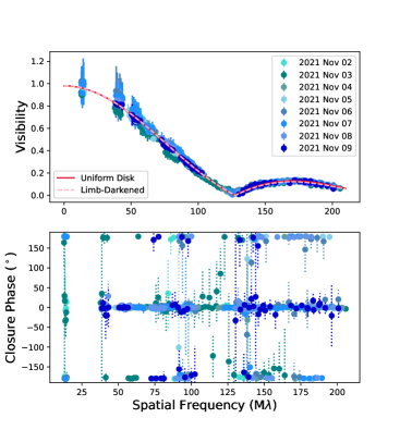
Figure 1: Plot (top) of normalized visibility amplitude versus spatial frequency ($B_{\bot}/\lambda$). The data combines all eight nights of observation for a total of 613 data points. Plot (bottom) of closure phases for all eight nights of observation, showing non-zero phases.

As a star is not expected to be a uniform disk, but should exhibit limb-darkening, the data were also fit to a power-law limb-darkened model,

$$I(\mu)=I_{0}\mu^{\alpha},$$ (2)

where $I$ is intensity, $I_{0}$ is the intensity at the center of the stellar disk, $\mu$ is the cosine of the angle from the observer to the normal to the stellar surface, and $\alpha$ is the limb-darkening coefficient. Hestroffer (1997) showed that this modifies the visibility amplitude, $V$, to be

$$V=(\alpha+2)\int_{0}^{1}\!(1-r^{2})^{\alpha/2}\ J_{0}(rB_{\bot}/\lambda)\ r\,\mathrm{d}r,$$ (3)

where $J_{0}$ is the Bessel function of the zeroth order of the first kind and $r$ is the fractional radius of the star.

Fitting for the angular diameter, we determine it to be $\theta_{\mathrm{LD}}$ = $2.019\pm 0.012$ mas with $V_{0}=$ $0.983\pm 0.011$ mas and $\alpha=$ $0.14\pm 0.03$. The value for $\alpha$ is consistent with values reported by Kervella et al. (2017) for similar stars: $\alpha$ Centauri A (G2V), $\alpha=0.1404\pm 0.0050$; $\alpha$ Centauri B (K1V), $\alpha=0.1545\pm 0.0044$; and the Sun, $\alpha=0.15027$.

For both the uniform and limb-darkened disks, the values presented here have had a factor of $1.0054\pm 0.0006$ divided from them, in accordance with a scaling found by Gardner et al. (2022) and an update by J. Monnier (private communication).

Both our uniform disk result ($1.979\pm 0.006$ mas) and our limb-darkened result ($2.019\pm 0.012$ mas) are within the range of previous literature values, seen in Table 4. Discrepancies are likely due to the amount or quality of the data used in the analyses. The measurement given here used significantly more data than those from the literature, both due to using all six CHARA Array telescopes and multiple nights of observation.

Using the Gaia parallax of $\pi=$ $273.8097\pm 0.1701$ mas (distance, $d=$ $3.652\pm 0.003$ parsecs (pc); Gaia Collaboration et al., 2022), we determine $\tau$ Ceti has a radius of $R=$ $0.793\pm 0.004$ $R_{\odot}$.

In the following calculations, we use the limb-darkened disk angular diameter and resultant radius estimate.

3.2 Temperature

We analyzed all of the EXPRES spectra following the procedure of Brewer et al. (2016) to derive abundances and global stellar parameters, including $T_{\mathrm{eff}}$, $\log{g}$, metallicity, rotational broadening, and projected rotational velocity ($v\sin{i}$), along with abundances for a few $\alpha$-elements. In this first stage, other abundances are scaled solar values. We then perturb the resulting temperature by $\pm 100$ K and re-fit. The global parameters from the weighted mean of the three models are fixed while abundances for 15 elements are fit. This new abundance pattern is adopted and the above two steps are repeated to get a final model.

From the EXPRES spectra and the analysis described, we determine an effective temperature of $T_{\mathrm{eff}}=$ $5320\pm 40$  K for $\tau$ Ceti.

The effective temperature can also be calculated from the angular diameter and bolometric flux with the relation

$$T_{\mathrm{eff}}=\left(\frac{4F_{\mathrm{bol}}}{\sigma\theta_{\mathrm{LD}}^{2}}\right)^{1/4}$$ (4)

where $F_{\mathrm{bol}}$ is the bolometric flux and $\sigma$ is the Stefan-Boltzmann constant. For the bolometric flux, we used the value for $\tau$ Ceti determined by Boyajian et al. (2013), $F_{\mathrm{bol}}=(112.60000\pm 0.0787)\times 10^{-8}$ erg s^-1 cm^-2. This gives $T_{\mathrm{eff}}=5370\pm 20$ K. The 1-$\sigma$ errors of this and the EXPRES $T_{\mathrm{eff}}$ overlap, showing agreement.

3.3 Projected Rotational Velocity from Spectra

During this spectral fitting, the “total rotational broadening” $v_{\mathrm{rot}}$ is the combined broadening from $v\sin{i}$ and macroturbulence, $v_{\mathrm{mac}}$. The two different broadening kernels are similar, although $v\sin{i}$ can be thought of as being nearly constant on vertical slices parallel to the spin axis of the star, whereas $v_{\mathrm{mac}}$ is nearly constant in annuli centered on the star. This is due to the varying radial and tangential components of the bulk motion caused by convection. Microturbulence, Doppler broadening due to lower velocity thermal motions, is fixed at 1 km s^-1 in this analysis.

Brewer et al. (2016) derived a macrotubulence relation as a function of $T_{\mathrm{eff}}$ for both dwarf stars and subgiants from their sample of $\sim 1600$ stars observed with Keck HIRES. They did this by assuming that the floor of the distribution of $v_{\mathrm{rot}}$ would be pole-on or non-rotating stars. The analysis then fixes the parameters derived from the first two stages, fixes $v_{\mathrm{mac}}$ using the relation, and fits for $v\sin{i}$.

$\tau$ Ceti was included as part of the Brewer et al. (2016) analysis, but it was an outlier with all five spectra analyzed having total rotational broadening 1.5 $\sigma$ below the floor of the distribution. Although the same procedure was used to analyze the EXPRES spectra, including the same line list, differences in the instrumental profile and spectral format can result in small differences between instruments. In general, stellar parameters between stars in common between the two instruments agreed within the uncertainties. The mean of the EXPRES measurements were $v_{\mathrm{rot}}=2.14\pm 0.05$ km s^-1. This still falls below the mean of the macrotubulence relation of Brewer et al. (2016). The final fitting stage then resulted in $v\sin{i}=0.08\pm 0.03$ km s^-1. Due to the uncertainty arising from the modeling, a more reasonable uncertainty would be 0.1 km s^-1, or about double the standard deviation in $v_{\mathrm{rot}}$. We use $v\sin i$ = $0.1\pm 0.1$ km s^-1 for our further analyses of $\tau$ Ceti.

We performed an additional test to verify that the $v\sin{i}$ was consistent with zero. We performed the same analysis described above on a total of 2,934 $\tau$ Ceti spectra from CHIRON (Tokovinin et al., 2013), EXPRES, and HARPS. No attempt was made to normalize the resulting parameters between the different spectrographs, since the parameters generally agreed to within the uncertainties. The resulting rotational broadening was $v_{\mathrm{rot}}=2.19\pm 0.07\ \mbox{km s${}^{-1}$}$, falling below the relation from Brewer et al. (2016) for $T_{\mathrm{eff}}\gtrsim 5280$ K, lower than the EXPRES value of $T_{\mathrm{eff}}=$ $5320\pm 40$  K (see Figure 2).

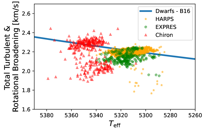
Figure 2: Total rotational broadening of 2934 spectra of $\tau$ Ceti from three different spectrographs. The Chiron spectra (red) show a bimodal distribution caused by poor characterization of the instrumental profile when using the fiber slicer versus the slit, which has a higher resolution. The dwarf macroturbulence relation from Brewer et al. (2016) (blue line) shows that, for most of the spectra, there is no appreciable rotation beyond that likely due to macroturbulence, resulting in our low estimate of $v\sin i$ = $0.1\pm 0.1$km s^-1.

3.4 Age

Age estimates for $\tau$ Ceti range from 4.4–12.4 Gyr (Lachaume et al., 1999; Pijpers et al., 2003; Di Folco et al., 2004; Mamajek & Hillenbrand, 2008; Baum et al., 2022). The values from Lachaume et al. (1999); Pijpers et al. (2003); Mamajek & Hillenbrand (2008); Baum et al. (2022) all depend upon estimates for the rotation period, $P_{\mathrm{rot}}$. However, with a $v\sin i=$ $0.1\pm 0.1$ km s^-1, which is consistent with little to no rotational velocity—potentially an indication of a pole-on orientation—we aim to investigate $\tau$ Ceti without the assumption that a periodic signal requiring rotation modulation has been detected. Di Folco et al. (2004) does not use a rotation period but rather a stellar evolution code that takes mass, luminosity, effective temperature, and initial chemical abundance as input. They give an age estimate of 10 Gyr.

3.5 Rotation Period and Inclination

With gyrochronology, the age of the star, rotation period, and color index are related. As derived in Barnes (2007), the age of the star can be expressed as follows:

$$\log{t}=\frac{1}{n}\left(\log{P_{\mathrm{rot}}}-\log{a}-b\log{((B-V)-0.4)}\right),$$ (5)

where $t$ is the age of the star in Myr, parameters $a$, $b$, and $n$ are constants, $P_{\mathrm{rot}}$ is the rotation period in days, and $B-V$ is the color index of the star. The constants are determined by Barnes (2007) to be $a=0.7725\pm 0.011$, $b=0.601\pm 0.024$, and $n=0.5189\pm 0.0070$. $B-V=0.72$ for $\tau$ Ceti (Ducati, 2002).

Using the age estimate from Di Folco et al. (2004) in Equation 5 and solving for the rotation period, we find $P_{\mathrm{rot}}=$ $46\pm 4$ days.

To determine the inclination of $\tau$ Ceti, we use the range of rotation periods based on the age range from Di Folco et al. (2004), the gyrochronology relationship given in Equation 5, the interferometrically determined stellar radius, and the spectroscopic $v\sin i$ to give an inclination of $7\pm 7^{\circ}$.

With this range of inclinations, rotational variations may be visible, but only on the stellar limb. We investigate possible indications of the rotation period of $\tau$ Ceti.

We note that the periodograms in the next three subsections led to a few peaks nearly equal in power. The strongest peaks for each are consistent with a nearly-pole-on orientation and we discuss those below.

3.5.1 MWO HK Project Rotation Period

We extracted a periodic signal from stellar chromospheric activity data from the MWO HK Project using a Lomb-Scargle periodogram. From this periodic signal, which we assume is due to rotation, we determined the rotation period to be $32\pm 9$ days, as seen in Figure 3. The errors were calculated using the bootstrap method, where we selected 1,784 points with replacement and found the best-fit $P_{\mathrm{rot}}$ 1,000 times. The standard deviation of those 1,000 iterations is the 9-day error. This relatively large error of 9 days is consistent with the fact that other significant peaks seen in the periodogram are included within this range. The false alarm probability of the peak in the periodogram is 0.004, indicating that the peak is statistically significant. Since a period was detected with significance, an inclination slightly larger than $0^{\circ}$ is suggested, consistent with the results described above. If this is the case, it implies that the periodic signal extracted from the data could be attributed to a rotational surface feature, such as starspots. This agrees with prior values from the literature of $34$ days (Baliunas et al., 1996), which uses the previous processing of the MWO data set, and $34.5$ days (Saar & Osten, 1997), which uses Ca II flux modulations.

Combining our MWO rotation period and rotational velocity, we determined the star’s inclination to be $5\pm 5$^∘. Other peaks within the errors of the rotation period lead to inclinations within the errors of $5\pm 5$^∘. The relatively weak signals in the periodogram are consistent with the pole-on inclination of the star, as the low inclination makes the rotation difficult to detect. Other comparatively strong peaks, such as that at $45$ days, are not far from the $P_{\mathrm{rot}}$ we derived with an age of $10$ Gyr.

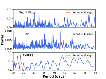
Figure 3: Periodogram created by chromospheric data from the Mount Wilson Observatory HK Project, photometric data from the Automatic Photoelectric Telescope at the Fairborn Observatory, and RV data from EXPRES. The red line shows the rotation period of the star at 32 days (MWO), 43 days (APT), and 23 days (EXPRES).

3.5.2 APT Rotation Period

We performed a periodogram analysis of the ground-based APT data to determine the rotation period of $\tau$ Ceti, $P_{\mathrm{rot}}=43\pm 7$ days. The errors were determined through the bootstrap method where 1,000 light curves containing 1,369 points (the number of points in the observed APT light curve) were randomly chosen with replacement. The power in the periodogram is very low, and there are several comparable peaks at other periods, including 35 days, which is consistent with our MWO $P_{\mathrm{rot}}$. Using our radius and $v\sin i$ values, the inclination is calculated to be $6\pm 6^{\circ}$ for a rotation period of $43\pm 7$ days.

While these results are consistent with our analyses described above, we note that the peaks in the periodogram are weak. The false-alarm probability of all peaks in this periodogram is near 1, which is consistent with a pole-on star and little rotational variation.

3.5.3 EXPRES RV Rotation Period

We performed a periodogram analysis on the EXPRES RVs to determine a rotation period. There were, however, no strong signals in this data set (see Figure 3). The strongest peak in the EXPRES data is found at 23 days and gives $i=3\pm 3^{\circ}$. It is possible with a longer temporal baseline of monitoring that a signal associated with the rotation period may be detected with more significance.

3.6 Surface Gravity

Like the values for $v\sin i$ and $T_{\mathrm{eff}}$, surface gravity, $\log g$, is determined from EXPRES data and model fitting described above in Section 3.3. These give a value of $\log g=$ $4.48\pm 0.05$.

3.7 Mass

From $\log g=$ $4.48\pm 0.05$ and the interferometric radius, we find a mass of $0.69\pm 0.09$ $M_{\odot}$.

A star’s mass can also be calculated using asteroseismic scaling relations for $\nu_{\mathrm{max}}$ and $\Delta\nu$:

$$\nu_{\mathrm{max}}=\left(\frac{M}{M_{\odot}}\right)\left(\frac{R}{R_{\odot}}\right)^{-2}\left(\frac{T}{T_{\odot}}\right)^{-1/2}\nu_{\mathrm{max}\odot}$$ (6)

and

$$\Delta\nu=\left(\frac{M}{M_{\odot}}\right)^{1/2}\left(\frac{R}{R_{\odot}}\right)^{-3/2}\Delta\nu_{\odot},$$ (7)

where $M$, $R$, and $T$ are the mass, radius, and temperature of $\tau$ Ceti, respectively. $M_{\odot}$, $R_{\odot}$, and $T_{\odot}$ are the solar values for these parameters. We used solar asteroseismic values from Huber et al. (2011) and $\tau$ Ceti’s asteroseismic values from Teixeira et al. (2009): $\nu_{\mathrm{max}}=4100\ \mu$Hz and $\Delta\nu=169\ \mu$Hz. Thus, from the frequency of maximum power and effective temperature $5320\pm 40$ K and the limb-darkened radius of $0.793\pm 0.004$ mas determined above, we calculate $\tau$ Ceti’s mass to be $0.800\pm 0.008$ $M_{\odot}$. From the large frequency separation and the limb-darkened radius, the mass is calculated to be $0.780\pm 0.012$ $M_{\odot}$, which is within the $1\sigma$ error of our mass derived above. These values are also consistent with literature values, which average around $0.78\ M_{\odot}$ (see values in Table 4 in the Appendix). The mass errors were calculated using the standard deviation of masses calculated by randomly picking a value from the Gaussian distribution of the other terms’ errors.

4 Dynamical Stability

The new constraints on the inclination of the stellar spin axis presented in this work have significant consequences for RV planets detected in the $\tau$ Ceti system. Feng et al. (2017) and Tuomi (2013) reported the discovery of four exoplanets orbiting $\tau$ Ceti, with orbital periods in the range of 20–636 days and semi-major axes of 0.133–1.334 AU, interior to the debris disk reported by MacGregor et al. (2016). The planets are reported to have masses ($m\sin i$) in the range of 1.75–3.93 $M_{\oplus}$. The reported planetary masses are minimum masses for the specific case of co-planar orbits that are aligned with the line of sight ($i=90^{\circ}$). It has been suggested that the planets are rocky and that additional planets may exist in the system within the orbital gaps (Dietrich & Apai, 2021). However, assuming that the planetary orbits are co-planar (Masuda et al., 2020) and possess a low obliquity with respect to the stellar spin axis (Albrecht et al., 2022), which is likely given the age of the system, the results presented in this paper imply a dramatic increase in the planetary masses. For example, inclinations of $i=6^{\circ}$ and $i=1^{\circ}$ increase the planetary masses by factors of $\sim$10 and $\sim$60, respectively. This means that the four known planets are likely substantially more massive than the minimum masses provided by Feng et al. (2017), such that they are not terrestrial in nature with masses that exceed that of Uranus and Neptune.

Given the planetary mass increase, we conducted a suite of dynamical simulations to test the dynamical integrity of the system. The N-body integrations were performed via the Mercury Integrator Package (Chambers, 1999) using methodology similar to that described by Kane (2015, 2016, 2019). Based upon our inclination range, we investigated orbital inclinations in the range 1–10$\arcdeg$ in steps of 1^∘, adjusting the Feng et al. (2017) planetary masses accordingly. Each simulation was run for $10$ Myr. Based on the inner planet orbital period of 20 days, we adopted a conservative time step for the simulations of 0.1 days to assure perturbative reliability. As quantified by Duncan et al. (1998), the time step should be, at minimum, 1/20 of the shortest orbital period; our time step is 1/200. Our simulations show that there is a significant transfer of angular momentum that occurs between the planets with all simulations that increases the eccentricity range of the planets compared to the initial values, suggesting that long-term stability is unlikely to be viable within the tested inclination regime. Importantly, the system is rendered unstable in less than $0.1$ Myr for the case of $i=1^{\circ}$ of both the star and the planets, implying that the planetary architecture described by Feng et al. (2017) cannot exist for that inclination scenario. Due to uncertainties in the orbital parameters, there is limited reliability in the dynamical simulation results when integrating beyond $10$ Myr. For simulations run for $10$ Myr with an inclination of $7^{\circ}$, the planets are nearing the instability threshold suggesting that, given more time, the system would also become unstable.

A face-on inclination for the $\tau$ Ceti system increases its viability as a direct imaging target from the perspective of planetary orbit visibility (Kane, 2013; Dulz et al., 2020). Direct imaging observations of the system thus far have placed upper limits on the presence of giant planets at large separations from the host star (Pathak et al., 2021). Further observations with the Roman Space Telescope will provide valuable additional constraints on possible giant planets present in the system (Turnbull et al., 2021).

5 Conclusion

We revised stellar parameters for $\tau$ Ceti with the assistance of new optical interferometric and spectroscopic data. Building upon fundamental observations, we formed a consistent picture of $\tau$ Ceti that shows it is nearly pole-on. As a result of the inclination, there are difficulties in reliably determining a rotation period and detecting planets with any method other than potentially future direct imaging. The orientation of the stellar rotation axis makes the detection of surface features like starspots difficult because their rotational modulations will only be detectable should they be nearly equatorial to allow for rotation over the stellar limb. This alignment also makes observing transits or RV shifts unlikely, unless the planets are significantly misaligned with the stellar rotation axis.

Because the potential planets described by Feng et al. (2017) fall between 0.133-1.33 AU, we assumed that their orbital plane would be aligned with the stellar rotation axis in our analysis in Section 4. While still within 3-$\sigma$ errors, our nearly pole-on inclination of $7\pm 7^{\circ}$ differs from the debris disk inclination of $35\pm 10^{\circ}$ (Lawler et al., 2014), which used observations from the Herschel satellite and had a beam size comparable to the size of the debris disk. A more recent study with ALMA data (MacGregor et al., 2016) assumed the inclination of $35^{\circ}$ from Lawler et al. (2014) and did not provide an independent fit to either the ALMA or Herschel data. If the difference in inclinations is real, this could imply that the disk and potential planets are misaligned with the star, or—since the debris disk result agreed with previous stellar inclination measurements of $0-40^{\circ}$ (Greaves et al., 2004)—it could suggest that a more accurate measurement of the debris disk inclination would be consistent with our pole-on stellar inclination. The possible misalignment between the stellar rotation axis and the debris disk potentially indicates a complicated formation scenario.

More interferometric observations would allow for imaging of the stellar surface potentially to see the rotation of surface structures, which may not modulate photometric or spectroscopic observations. Our current data, however, are not sufficient for imaging, as it is too limited in $uv$ coverage and time. A new set of data obtained during a single stellar rotation would allow for the unambiguous confirmation of the stellar inclination and help place limits on the spottedness of the stellar surface. Observations taken throughout the stellar rotation, maximizing the $uv$ coverage across the stellar surface and with sufficient resolution to resolve surface features can be obtained with the six-telescope beam combiners at the CHARA Array. While MIRC-X can provide these capabilities in $H$-band, the Stellar Parameters and Images with a Cophased Array (SPICA) beam combiner (Mourard et al., 2022) will operate in optical wavelengths and will soon be available to the public. SPICA will provide the opportunity to achieve higher-resolution images of stellar surfaces than is currently possible. Such a precise new data set is needed to improve upon our results and is necessary for characterizing both the star and any planets it hosts.

Appendix A Literature Table

For a detailed comparison of the values determined by the methods described above, we include the stellar parameters determined by previous studies. In Table 4, we include literature values and notes on how those values were obtained.

Table 4: Recent $\tau$ Ceti Literature Values

Reference	Temperature	Mass	Radius	Luminosity	Age	Angular	Angular	Method
	(K)	($M_{\odot}$)	($R_{\odot}$)	($L_{\odot}$)	(Gyr)	Diameter	Diameter
						(mas; UD)	(mas; LD)
This work	$5320\pm 40$	$0.69\pm 0.09$	$0.793\pm 0.004$	$0.45\pm 0.02$	–	$1.979\pm 0.006$	$2.019\pm 0.012$	interferometry + spectroscopy
Baum et al. (2022)	5333	0.990	–	–	12.4	–	–	spectroscopy
Tabernero et al. (2021)	$5400\pm 60$	$0.760\pm.017$	$0.750\pm.015$	–	–	–	–	spectroscopic modelling
Esposito et al. (2020)	5750	$0.85\pm.01$	0.75	$0.56\pm 0.23$	–	–	–	optical photometry
Rains et al. (2020)	$5347\pm 18$	–	$0.796\pm.004$	$0.47\pm 0.01$	–	$2.005\pm 0.011$	$2.054\pm 0.011$	interferometry + flux
Chaplin et al. (2019)	5290	0.79	0.85	0.51	–	–	–	spectroscopy
Kervella et al. (2019)	–	$0.900\pm.045$	$0.751\pm.014$	–	–	–	–	isochrone fitting + surface
								brightness-color relation
France et al. (2018)	$5340\pm 36$	–	$0.793\pm.036$	–	–	–	–	spectral type
Fuhrmann et al. (2017)	–	0.78	–	–	–	–	–	stellar evolutionary track
Brewer et al. (2016)	$5344\pm 60$	$0.78\pm.02$	0.82	–	–	–	–	spectroscopy
Heiter et al. (2015)	$5326\pm 45$	$0.71\pm.03$	–	$0.447\pm 0.005$	–	–	–	spectroscopy + isochrone
Pagano et al. (2015)	5387	0.78	0.69	0.504	–	–	–	spectroscopy
Baines et al. (2014)	–	–	–	–	–	$1.952\pm 0.003$	$2.072\pm 0.010$	interferometry
Absil et al. (2013)	–	–	–	–	–	–	$2.015\pm 0.004$	interferometry
Boyajian et al. (2013)	$5290\pm 39$	0.733	$0.815\pm.012$	$0.4674\pm 0.0007$	–	–	–	parallax/flux + isochrone
Jofre et al. (2013)	$5414\pm 21$	$0.78\pm.01$	0.69	–	–	–	–	spectroscopy
Tang & Gai (2011)	5409	0.775	0.790	0.47985	–	–	–	asteroseismology model 1
Tang & Gai (2011)	5387	0.785	0.793	0.47612	–	–	–	asteroseismology model 2
Tang & Gai (2011)	$5264\pm 100$	–	0.87	$0.52\pm 0.03$	–	–	–	spectroscopy
Tang & Gai (2011)	$5525\pm 12$	–	0.77	$0.50\pm 0.006$	–	–	–	spectroscopy + interferometry
Bruntt et al. (2010)	$5383\pm 47$	$0.79\pm.03$	$0.794\pm.005$	$0.47\pm 0.02$	–	–	–	interferometry + photometry
Teixeira et al. (2009)	5418	$0.783\pm.012$	$0.793\pm.004$	$0.488\pm 0.010$	–	–	–	parallax + asteroseismology
Mamajek & Hillenbrand (2008)	–	–	–	–	5.8	–	–	activity-rotation
Sousa & Cunha (2008)	$5310\pm 17$	0.627	0.62	$0.495\pm 0.003$	–	–	–	spectroscopy
di Folco et al. (2007)	5400	0.72	$0.790\pm.005$	–	–	–	–	parallax
Di Folco et al. (2004)	$5264\pm 100$	$0.85\pm.14$	$0.806\pm.013$	–	–	$2.005\pm 0.034$	–	spectrophotometry + interferometry
Di Folco et al. (2004)	5377	0.83	0.821	–	10	–	–	stellar evolutionary track
Pijpers et al. (2003)	$5264\pm 100$	0.50	$0.773\pm.004$	$0.52\pm 0.03$	9-10	$1.933\pm 0.009$	$1.971\pm 0.009$	interferometry + spectroscopy

Note. — Some references are listed multiple times, as multiple methods were used to determine the stellar parameters

References

- Absil et al. (2013) Absil, O., Defrère, D., Coudé du Foresto, V., et al. 2013, A&A, 555, A104, doi: 10.1051/0004-6361/201321673
- Adams (1916) Adams, W. S. 1916, PASP, 28, 279, doi: 10.1086/122555
- Albrecht et al. (2022) Albrecht, S. H., Dawson, R. I., & Winn, J. N. 2022, PASP, 134, 082001, doi: 10.1088/1538-3873/ac6c09
- Anugu et al. (2020) Anugu, N., Le Bouquin, J.-B., Monnier, J. D., et al. 2020, AJ, 160, 158, doi: 10.3847/1538-3881/aba957
- Astropy Collaboration et al. (2013) Astropy Collaboration, Robitaille, T. P., Tollerud, E. J., et al. 2013, A&A, 558, A33, doi: 10.1051/0004-6361/201322068
- Astropy Collaboration et al. (2018) Astropy Collaboration, Price-Whelan, A. M., Sipőcz, B. M., et al. 2018, AJ, 156, 123, doi: 10.3847/1538-3881/aabc4f
- Baines et al. (2014) Baines, E. K., Armstrong, J. T., Schmitt, H. R., et al. 2014, ApJ, 781, 90, doi: 10.1088/0004-637X/781/2/90
- Baliunas et al. (1996) Baliunas, S., Sokoloff, D., & Soon, W. 1996, ApJ, 457, L99, doi: 10.1086/309891
- Baliunas et al. (1995) Baliunas, S. L., Donahue, R. A., Soon, W. H., et al. 1995, ApJ, 438, 269, doi: 10.1086/175072
- Barnes (2007) Barnes, S. A. 2007, ApJ, 669, 1167, doi: 10.1086/519295
- Baum et al. (2022) Baum, A. C., Wright, J. T., Luhn, J. K., & Isaacson, H. 2022, AJ, 163, 183, doi: 10.3847/1538-3881/ac5683
- Blackman et al. (2020) Blackman, R. T., Fischer, D. A., Jurgenson, C. A., et al. 2020, AJ, 159, 238, doi: 10.3847/1538-3881/ab811d
- Boyajian et al. (2013) Boyajian, T. S., von Braun, K., van Belle, G., et al. 2013, ApJ, 771, 40, doi: 10.1088/0004-637X/771/1/40
- Brewer et al. (2016) Brewer, J. M., Fischer, D. A., Valenti, J. A., & Piskunov, N. 2016, ApJS, 225, 32, doi: 10.3847/0067-0049/225/2/32
- Bruntt et al. (2010) Bruntt, H., Bedding, T. R., Quirion, P. O., et al. 2010, MNRAS, 405, 1907, doi: 10.1111/j.1365-2966.2010.16575.x
- Chambers (1999) Chambers, J. E. 1999, MNRAS, 304, 793, doi: 10.1046/j.1365-8711.1999.02379.x
- Chaplin et al. (2019) Chaplin, W. J., Cegla, H. M., Watson, C. A., Davies, G. R., & Ball, W. H. 2019, AJ, 157, 163, doi: 10.3847/1538-3881/ab0c01
- Chelli et al. (2016) Chelli, A., Duvert, G., Bourgès, L., et al. 2016, A&A, 589, A112, doi: 10.1051/0004-6361/201527484
- Di Folco et al. (2004) Di Folco, E., Thévenin, F., Kervella, P., et al. 2004, A&A, 426, 601, doi: 10.1051/0004-6361:20047189
- di Folco et al. (2007) di Folco, E., Absil, O., Augereau, J. C., et al. 2007, A&A, 475, 243, doi: 10.1051/0004-6361:20077625
- Dietrich & Apai (2021) Dietrich, J., & Apai, D. 2021, AJ, 161, 17, doi: 10.3847/1538-3881/abc560
- Ducati (2002) Ducati, J. R. 2002, VizieR Online Data Catalog
- Dulz et al. (2020) Dulz, S. D., Plavchan, P., Crepp, J. R., et al. 2020, ApJ, 893, 122, doi: 10.3847/1538-4357/ab7b73
- Duncan et al. (1991) Duncan, D. K., Vaughan, A. H., Wilson, O. C., et al. 1991, ApJS, 76, 383, doi: 10.1086/191572
- Duncan et al. (1998) Duncan, M. J., Levison, H. F., & Lee, M. H. 1998, AJ, 116, 2067, doi: 10.1086/300541
- Esposito et al. (2020) Esposito, T. M., Kalas, P., Fitzgerald, M. P., et al. 2020, AJ, 160, 24, doi: 10.3847/1538-3881/ab9199
- Feng et al. (2017) Feng, F., Tuomi, M., Jones, H. R. A., et al. 2017, AJ, 154, 135, doi: 10.3847/1538-3881/aa83b4
- France et al. (2018) France, K., Arulanantham, N., Fossati, L., et al. 2018, ApJS, 239, 16, doi: 10.3847/1538-4365/aae1a3
- Fuhrmann et al. (2017) Fuhrmann, K., Chini, R., Kaderhandt, L., & Chen, Z. 2017, ApJ, 836, 139, doi: 10.3847/1538-4357/836/1/139
- Gaia Collaboration et al. (2022) Gaia Collaboration, Klioner, S. A., Lindegren, L., et al. 2022, arXiv e-prints, arXiv:2204.12574. https://arxiv.org/abs/2204.12574
- Gardner et al. (2022) Gardner, T., Monnier, J. D., Fekel, F. C., et al. 2022, AJ, 164, 184, doi: 10.3847/1538-3881/ac8eae
- Ginsburg et al. (2019) Ginsburg, A., Sipőcz, B. M., Brasseur, C. E., et al. 2019, AJ, 157, 98, doi: 10.3847/1538-3881/aafc33
- Greaves et al. (2004) Greaves, J. S., Wyatt, M. C., Holland, W. S., & Dent, W. R. F. 2004, MNRAS, 351, L54, doi: 10.1111/j.1365-2966.2004.07957.x
- Handler (2013) Handler, G. 2013, in Planets, Stars and Stellar Systems. Volume 4: Stellar Structure and Evolution, ed. T. D. Oswalt & M. A. Barstow, Vol. 4, 207, doi: 10.1007/978-94-007-5615-1_4
- Harris et al. (2020) Harris, C. R., Millman, K. J., van der Walt, S. J., et al. 2020, Nature, 585, 357, doi: 10.1038/s41586-020-2649-2
- Heiter et al. (2015) Heiter, U., Jofré, P., Gustafsson, B., et al. 2015, A&A, 582, A49, doi: 10.1051/0004-6361/201526319
- Henry (1999) Henry, G. W. 1999, PASP, 111, 845, doi: 10.1086/316388
- Hestroffer (1997) Hestroffer, D. 1997, A&A, 327, 199
- Huber et al. (2011) Huber, D., Bedding, T. R., Stello, D., et al. 2011, ApJ, 743, 143, doi: 10.1088/0004-637X/743/2/143
- Hunter (2007) Hunter, J. D. 2007, Computing in Science & Engineering, 9, 90, doi: 10.1109/MCSE.2007.55
- Jofre et al. (2013) Jofre, R., Brito-Castillo, L., Tereshchenko, I., & Atmospheric Sciences Climatology Climate Variability. 2013, in AGU Spring Meeting Abstracts, Vol. 2013, A31A–08
- Kane (2013) Kane, S. R. 2013, ApJ, 766, 10, doi: 10.1088/0004-637X/766/1/10
- Kane (2015) —. 2015, ApJ, 814, L9, doi: 10.1088/2041-8205/814/1/L9
- Kane (2016) —. 2016, ApJ, 830, 105, doi: 10.3847/0004-637X/830/2/105
- Kane (2019) —. 2019, AJ, 158, 72, doi: 10.3847/1538-3881/ab2a09
- Keenan & McNeil (1989) Keenan, P. C., & McNeil, R. C. 1989, ApJS, 71, 245, doi: 10.1086/191373
- Kervella et al. (2019) Kervella, P., Arenou, F., Mignard, F., & Thévenin, F. 2019, A&A, 623, A72, doi: 10.1051/0004-6361/201834371
- Kervella et al. (2017) Kervella, P., Bigot, L., Gallenne, A., & Thévenin, F. 2017, A&A, 597, A137, doi: 10.1051/0004-6361/201629505
- Kjeldsen & Bedding (1995) Kjeldsen, H., & Bedding, T. R. 1995, A&A, 293, 87. https://arxiv.org/abs/astro-ph/9403015
- Kopparapu (2014) Kopparapu, R. 2014, in Habitable Worlds Across Time and Space, 25
- Lachaume et al. (1999) Lachaume, R., Dominik, C., Lanz, T., & Habing, H. J. 1999, A&A, 348, 897
- Lawler et al. (2014) Lawler, S. M., Di Francesco, J., Kennedy, G. M., et al. 2014, MNRAS, 444, 2665, doi: 10.1093/mnras/stu1641
- MacGregor et al. (2016) MacGregor, M. A., Lawler, S. M., Wilner, D. J., et al. 2016, ApJ, 828, 113, doi: 10.3847/0004-637X/828/2/113