How Gubser flow ends in a holographic conformal theory

Abstract

Gubser flow is an axis-symmetric and boost-invariant evolution in a relativistic quantum field theory, providing a model for the evolution of matter produced in the wake of heavy-ion collisions. It is best studied by mapping $\mathbf{R}^{3,1}$ to $dS_{3}\times\mathbf{R}$ when the field theory has conformal symmetry. We show that at late de-Sitter time, which corresponds to large proper time and central region in the future wedge within $\mathbf{R}^{3,1}$, the holographic conformal field theory plasma can reach a state in which $\varepsilon=P_{T}=-P_{L}$, with $\varepsilon$, $P_{T}$ and $P_{L}$ being the energy density, transverse and longitudinal pressures, respectively. We also show that the general late de-Sitter time expansion can systematically determine both the Minkowksi early proper time behavior and the profile at large distance from the beam axis at any Minkowski proper time. Particularly, $\varepsilon=P_{T}=-P_{L}$ is also realized at early Minkowski proper time, and we can determine the initial conditions in such situations. Furthermore, we determine subleading corrections. Hydrodynamic modes appear at intermediate times.

I Introduction

Gubser flow Gubser (2010); Gubser and Yarom (2011) is a time-dependent evolution of a relativistic many-body system which is boost invariant and has a rotational symmetry about an axis. The original context of study of the Gubser flow is the evolution of QCD matter produced in central heavy ion collisions, in which case the axis of rotational symmetry is the beam axis.

Gubser flow in conformal field theory can be studied by mapping Minkowski space ($\mathbf{R}^{3,1}$) to a product of three dimensional de Sitter space and the real line ($dS_{3}\times\mathbf{R}$), which makes the symmetries manifest Gubser and Yarom (2011).The most remarkable feature of Gubser flow is that at late de Sitter time, $\rho$, the evolution cannot be described by relativistic hydrodynamics Gubser and Yarom (2011); Denicol et al. (2014a, b); Denicol and Noronha (2019); Chattopadhyay et al. (2019); Behtash et al. (2020); Dash and Roy (2020). This large $\rho$ regime is large proper time and the central region of the flow in Minkowski space.

Our study of the holographic Gubser flow sets a primary example in which one can exactly determine how a system can evolve out of hydrodynamic regime due to expansion of some directions of space in a quantum field theory, and is relevant to understanding evolution of quantum matter in Kasner geometries Berger (2002) describing spacetime singularities, etc.

In kinetic theories without particle production, it has been shown Denicol et al. (2014a, b); Denicol and Noronha (2019); Chattopadhyay et al. (2019); Behtash et al. (2020); Dash and Roy (2020) that the large $\rho$ behavior is free-streaming where inter-particle interactions disappear. However, such ultra dilute regime is better studied in quantum field theory. Here, we show that in a holographic conformal theory, the deconfined plasma can reach a phase in which the energy density $\varepsilon$, the transverse pressure $P_{T}$ and the longitudinal pressure $P_{L}$ satisfy $P_{L}=-P_{T}$, and $\varepsilon=P_{T}$ in the large $\rho$ limit indepedently of the details of the state of the system at an early time. Remarkably, this phase is similar to the color glass condensate regime described by perturbative physics of saturated gluons Epelbaum and Gelis (2013); Müller (2019); Berges et al. (2021).

Furthermore, we establish that the general late de Sitter time expansion can systematically determine both the early Minkowski proper time behavior and the behavior at large distance from the beam axis at any fixed Minkowski proper time. Particularly, the color glass condensate behavior $\varepsilon=P_{T}=-P_{L}$ is also realized at early proper time, as in actual heavy-ion collisions, while hydrodynamic modes appear at intermediate times.

II Preliminaries

For a conformal system on $\mathbf{R}^{3,1}$, the full symmetry of the Gubser flow is $SO(3)_{q}\otimes SO(1,1)\otimes Z_{2}$. These symmetries can be made manifest by performing diffeomorphism and Weyl rescaling of $\mathbf{R}^{3,1}$ to $dS_{3}\times\mathbf{R}$ Gubser and Yarom (2011). The $SO(1,1)$ boost symmetry acts additively and $Z_{2}$, the reflection symmetry about the collision plane, acts reflexively on the $\mathbf{R}$ factor, which is physically the rapidity. Furthermore, $dS_{3}$ is a contracting and then expanding $S^{2}$ on which $SO(3)$ has a natural action. The variable $q$ parametrizes inequivalent ways of embedding $SO(3)\otimes SO(1,1)$ in the full conformal group $SO(4,2)$. Also, $q^{-1}$ has the dimension of length and is essentially the size of the colliding systems.

The explicit map from $\mathbf{R}^{3,1}$ to $dS_{3}\times\mathbf{R}$ is via the Milne coordinates, which are the proper time $\tau=\sqrt{t^{2}-z^{2}}$, the rapidity $\eta={\rm arctan}(z/t)$, the radial coordinate $x_{\perp}$ and the angular coordinate $\phi$ of the plane transverse to the $z$-axis (the beam axis). In Milne coordinates, the metric on $\mathbf{R}^{3,1}$ is

$${\rm d}s^{2}=-{\rm d}\tau^{2}+\tau^{2}{\rm d}\eta^{2}+{\rm d}x_{\perp}^{2}+x_{\perp}^{2}{\rm d}\phi^{2}.$$ (1)

The $dS_{3}\times\mathbf{R}$ coordinates are $\rho$, $\theta$, $\phi$ and $\eta$, where

$$\rho = -L\,\,{\rm arcsinh}\left(\frac{1-q^{2}\tau^{2}+q^{2}x_{\perp}^{2}}{2q\tau}\right),$$ (2)

$$\theta = {\rm arctan}\left(\frac{2qx_{\perp}}{1+q^{2}\tau^{2}-q^{2}x_{\perp}^{2}}\right).$$ (3)

Crucially, the future wedge, which is the causal future of the plane of the collision at $\tau=0$, is contained in $dS_{3}\times\mathbf{R}$. The corresponding metric

$${\rm d}\hat{s}^{2} =\frac{L^{2}}{\tau^{2}}{\rm d}s^{2}$$ (4)

$$=-{\rm d}\rho^{2}+L^{2}\cosh^{2}\left(\frac{\rho}{L}\right)\left({\rm d}\theta^{2}+\sin^{2}\theta{\rm d}\phi^{2}\right)+L^{2}{\rm d}\eta^{2},$$

is Weyl equivalent to the flat metric. From our discussion above, it is clear that $\rho$ is invariant under $SO(3)_{q}\otimes SO(1,1)\otimes Z_{2}$, and therefore physical quantities like the energy density should depend only on $\rho$ explicitly up to the Weyl rescaling. We will denote physical quantities measured in $dS_{3}\times\mathbf{R}$ with a hat.

The conformal Ward identites for the energy-momentum tensor are:

$$\hat{\nabla}_{\mu}\hat{T}^{\mu}_{\,\,\nu}=0,\quad\hat{T}^{\mu}_{\,\,\mu}=\mathcal{A},$$ (5)

where $\mathcal{A}$ is the Weyl anomaly. The $SO(3)_{q}\otimes SO(1,1)\otimes Z_{2}$ symmetries and these Ward identities imply that $\hat{T}^{\mu}_{\nu}$ should be of the form

$$\hat{T}^{\mu}_{\,\,\nu}=\hat{t}^{\mu}_{\,\,\nu}+\hat{\mathcal{A}}^{\mu}_{\,\,\nu}$$ (6)

where

$$\hat{t}^{\rho}_{\,\,\rho}=-\hat{\varepsilon}\left(\frac{\rho}{L}\right),$$ (7)

$$\hat{t}^{\theta}_{\,\,\theta}=\hat{t}^{\phi}_{\,\,\phi}=\hat{P}_{T}(\rho)=-\frac{1}{2}\coth\left(\frac{\rho}{L}\right)\hat{\varepsilon}^{\prime}\left(\frac{\rho}{L}\right)-\hat{\varepsilon}\left(\frac{\rho}{L}\right),$$ (8)

$$\hat{t}^{\eta}_{\,\,\eta}=\hat{P}_{L}(\rho)=\coth\left(\frac{\rho}{L}\right)\hat{\varepsilon}^{\prime}\left(\frac{\rho}{L}\right)+3\hat{\varepsilon}\left(\frac{\rho}{L}\right).$$ (9)

Here, ^′ denotes a derivative w.r.t. to the argument. It is easy to check that $\hat{t}^{\mu}_{\,\,\nu}$ is separately conserved (i.e. $\hat{\nabla}_{\mu}\hat{t}^{\mu}_{\,\,\nu}=0$) and is traceless. The anomalous term $\hat{\mathcal{A}}^{\mu}_{\,\,\nu}$ (which is state-independent) is explicitly

$$\hat{\mathcal{A}}^{\mu}_{\,\,\nu}=\frac{N^{2}}{32\pi^{2}}{\rm diag}\left(1,1,1,-3\right)L^{-4}$$ (10)

for $\mathcal{N}=4$ $SU(N)$ super Yang-Mills-theory (SYM) Henningson and Skenderis (1998); Balasubramanian and Kraus (1999). We note that $\mathcal{A}=\hat{\mathcal{A}}^{\mu}_{\,\,\mu}=0$.

It is clear from the above that the only input from the microscopic dynamics that is needed to determine the energy-momentum tensor is the evolution of the energy density $\hat{\varepsilon}(\rho)$, because the latter determines the transverse pressure $\hat{P}_{T}$ and the longitudinal pressure $\hat{P}_{L}$ via (8) and (9), respectively. Weyl transformation yields the energy-momentum tensor in Minkowski space:

$${T}^{\mu}_{\,\,\nu}=\frac{L^{4}}{\tau^{4}}\hat{t}^{\mu}_{\,\,\nu},\,\,{\rm i.e.}\,\,\varepsilon=L^{4}\tau^{-4}\hat{\varepsilon}.$$ (11)

Note that the anomalous term disappears.

In the hydrodynamic regime, the general form of the energy-momentum tensor given by (7)-(9) implies that the fluid is static in the ${\rm d}S_{3}\times\mathbf{R}$ frame, i.e. the velocity field is of the form $\hat{u}^{\rho}=1$ with other components vanishing. The hydrodynamic equations determine $\hat{\varepsilon}(\rho)$. For a perfect conformal fluid, $\hat{\varepsilon}(\rho)=\hat{\varepsilon}_{0}\cosh^{-8/3}(\rho/L)$, whereas for a viscous flow (see Appendix A for an explicit solution), $\hat{\varepsilon}$ goes to a constant at large $\rho$ indicating the breakdown of the derivative expansion. However, at $\rho\sim 0$, the Knudsen number is small, and the derivative expansion is equivalent to

$$\hat{\varepsilon}(\rho)=\hat{\varepsilon}_{0}-\frac{4}{3}\hat{\varepsilon}_{0}\frac{\rho^{2}}{L^{2}}+\frac{16}{27}H_{0}\hat{\varepsilon}_{0}^{3/4}\frac{\rho^{3}}{L^{4}}+\mathcal{O}(\rho^{4}),$$ (12)

with $H_{0}$ being the dimensionless (and constant) shear viscosity (see Appendix A). This hydrodynamic evolution is only transitory.

III Holographic Gubser flow

Any state in the universal sector of a holographic conformal gauge theory, such as $\mathcal{N}=4$ SYM with $SU(N)$ gauge group, has a dual description as a solution of pure classical Einstein’s gravity with a negative cosmological constant in one higher spacetime dimension in infinite ’t Hooft coupling and large $N$ limits Maldacena (1998); Witten (1998); Gubser et al. (1998). Such a solution should be regular, i.e. without any naked singularity, and with boundary metric $g^{(b)}_{\mu\nu}$ defined in terms of the bulk metric $G_{\mu\nu}$ via

$$\lim_{r\rightarrow 0}\frac{r^{2}}{l^{2}}G_{\mu\nu}\equiv g^{(b)}_{\mu\nu},$$ (13)

coinciding with the physical background metric on which the gauge theory lives. Above, $r$ is the holographic radial coordinate, which has an interpretation in terms of the energy scale of the dual theory Freedman et al. (1999); Heemskerk and Polchinski (2011); Bredberg et al. (2011); Kuperstein and Mukhopadhyay (2011, 2013); Behr and Mukhopadhyay (2016); Behr et al. (2016); Mukhopadhyay (2016), while $\mu$ and $\nu$ indices represent the directions spanning the boundary of spacetime at $r=0$. The bulk cosmological constant is $\Lambda=-6/l^{2}$.

Any five-dimensional gravitational solution dual to a Gubser flow of the dual gauge theory in $dS_{3}\times\mathbf{R}$ can be written in the form

$${\rm d}s^{2}=-\frac{2l^{2}}{r^{2}}{\rm d}r{\rm d}\rho-\frac{l^{2}}{r^{2}}\left(1-\frac{r^{2}}{L^{2}}+A\left(\frac{r}{L},\frac{\rho}{L}\right)\right){\rm d}\rho^{2}$$

$$+\frac{l^{2}(L\cosh(\rho/L)+r\sinh(\rho/L))^{2}}{r^{2}}$$

$$\times e^{B\left(\frac{r}{L},\frac{\rho}{L}\right)}\,\Big{(}{\rm d}\theta^{2}+\sin^{2}\theta{\rm d}\phi^{2}\Big{)}$$

$$+\frac{l^{2}}{r^{2}}e^{C\left(\frac{r}{L},\frac{\rho}{L}\right)-2B\left(\frac{r}{L},\frac{\rho}{L}\right)}\,L^{2}{\rm d}\eta^{2}.$$ (14)

We have chosen the ingoing Eddington-Finkelstein gauge in which the regularity of the future horizon can be readily examined. For the boundary metric to be the metric (4) on ${\rm d}S_{3}\times\mathbf{R}$, we need

$$A(r=0,\rho/L)=B(r=0,\rho/L)=C(r=0,\rho/L)=0.$$ (15)

The solution dual to the vacuum state corresponds to $A=B=C=0.$ This solution is locally $AdS_{5}$. Generally, as detailed in Appendix B, $A$, $B$ and $C$ have radial expansions of the form

$$A=\sum_{n=0}^{\infty}a_{(n)}(\rho/L)\frac{r^{n}}{L^{n}},\,\,B=\sum_{n=0}^{\infty}b_{(n)}(\rho/L)\frac{r^{n}}{L^{n}},$$

$$C=\sum_{n=0}^{\infty}c_{(n)}(\rho/L)\frac{r^{n}}{L^{n}}$$ (16)

Plugging these in Einstein’s equation, we find that the entire solution is determined just by two inputs: $a_{(1)}(\rho/L)$, which is related to a proper residual diffeomorphism that does not affect the boundary data, and $a_{(4)}(\rho/L)$ which is physical and should be chosen such that no naked singularity is present.

Physically $a_{(4)}(\rho/L)$ determines with the energy-momentum tensor of the dual gauge theory state. The latter can be obtained systematically via the standard holographic dictionary (see Appendix B) Henningson and Skenderis (1998); Balasubramanian and Kraus (1999); de Haro et al. (2001); Skenderis (2002). Noting that $l^{3}/G_{N}=(2/\pi)N^{2}$ Maldacena (1998), we find that the dual energy-momentum tensor has the same form as that given by (6)-(10) (including the anomalous term) with the identification

$$\hat{\varepsilon}\left(\frac{\rho}{L}\right)=-\frac{3l^{3}}{16\pi G_{N}}a_{(4)}\left(\frac{\rho}{L}\right)=-\frac{3N^{2}}{8\pi^{2}}a_{(4)}\left(\frac{\rho}{L}\right).$$ (17)

Since a Weyl transformation at the boundary can be lifted to a bulk diffeomorphism Henningson and Skenderis (1998); de Haro et al. (2001), we can readily obtain the Minkowski boundary metric (1) and the energy-momentum tensor (11) via an appropriate bulk diffeomorphism.

IV Finding the late time solution in ${\rm d}S_{3}\times\mathbf{R}$

The problem of finding generic late time behavior amounts to setting up a suitable late time expansion and determining the set of conditions which lead to a regular future horizon in this expansion perturbatively. Furthermore, the solution has to be normalizable, i.e. satisfy (15). Due to the exponential expansion of $S^{2}$, the energy density in ${\rm d}S_{3}\times\mathbf{R}$ should dilute and we should eventually reach the vacuum. Therefore, in the dual gravitational solution (III), $A$, $B$ and $C$ must eventually vanish. The latter solution with $A=B=C=0$ has a horizon at $r=L$ where $\partial_{\rho}$ has vanishing norm. (Note this is not a Killing horizon.) Therefore at large $\rho$, the horizon should be at $r=L$ at leading order in the late time expansion, and just like in the case of fluid-gravity correspondence Rangamani (2009), we should require that at each order in the perturbative expansion, the behavior of $A$, $B$ and $C$ are smooth at $r=L$ implying regularity of the future horizon.

It is instructive to first discuss the example of a massless scalar field $\Phi$ which satisfies the Klein-Gordon equation $\nabla^{2}\Phi=0$, where $\nabla^{2}$ is the Laplacian operator in the five-dimensional metric (III) dual to the vacuum and with $A=B=C=0$. Demanding $SO(3)_{q}\otimes SO(1,1)\otimes Z_{2}$ symmetry amounts to requiring that $\Phi$ depends only on $r$ and $\rho$. It is easy to see that the background five dimensional metric is a rational function of $\sigma=\exp(\rho/L)$. Therefore, we will expect that at late time $\Phi(r,\rho)$ should behave as $\sigma^{-\alpha}\sim\exp(-\alpha\rho/L)$.The consistent ansatz which fits this late time behavior (at large $\sigma$) is

$$\Phi(r,\rho)=\sigma^{-\alpha}\sum_{n=0}^{\infty}\phi_{n}(v)\sigma^{-2n}$$ (18)

where $v=r/L$. However, if the solution is analytic at the horizon $r=L$, we should expect the behavior near $r=L$ (i.e. $v=1$) to be given by

$$\phi_{n}(v)=\sum_{m=0}^{\infty}\lambda_{n,m}(1-v)^{m},$$ (19)

where $\lambda_{n,m}$ are pure numbers. Substituting (18) and (19) in the Klein-Gordon equation, we can readily solve all other $\lambda_{n,m}$ in terms of $\lambda_{0,m}$ which can be chosen freely. Finally, we would require the condition of normalizability, i.e.

$$\phi_{n}(v=0)=0.$$ (20)

Solving $\lambda_{n,0}$ explicitly in terms of $\lambda_{0,0}$, we would get

$$\phi_{0}(v=0)=\lambda_{0,0}f_{0}(\alpha).$$ (21)

The allowed values of $\alpha$ are simply the roots of $f_{0}(\alpha)$. Solving for $\lambda_{n,0}$ to very high orders, we get stable roots, which are $4+2k$, for $k=0,1,2,\ldots$ From the ansatz (18) and the allowed values of $\alpha$, it follows that if $\phi_{0}$ is normalizable then so is $\phi_{n}$ for $n\geq 1$. Since $\phi_{0}$ determines the source term in the linear equation for $\phi_{1}$ (and so on) which produces a normalizable particular solution, and the boundary value of the homogeneous solution should vanish since it coincides with the leading order normalizable solution with $\alpha=4+2k$ for $k\geq 1$, it follows that the generic late time behavior is simply (18) with $\alpha=4$.

The expectation value (e.v.) of the marginal operator $\hat{O}$ in the gauge theory dual to the massless scalar field is essentially the $r^{4}$ coefficient in the radial expansion of $\Phi$. Ignoring backreaction of the dual bulk scalar field, the generic behavior of the vacuum e.v. of this operator with Gubser flow symmetries is thus

$$\hat{O}(\rho)\sim\sigma^{-4}\sum_{k=0}^{\infty}\hat{o}_{k}\sigma^{-2k},$$ (22)

where $\hat{o}_{k}$ are arbitrary real numbers.

The solutions for $\phi_{n}(v)$ turn out to be rational functions. Furthermore, with specific choices of particular solutions for the subleading $\phi_{n}$, we can sum over the entire late time expansion as well. For instance, when the leading behaviour is $\sigma^{-4}$ (i.e. $\hat{o}_{4}\neq 0$), the full summation yields

$$\Phi(r,\rho)=\Gamma_{4}\frac{\sigma^{-4}v^{4}}{(1+v)^{5}}\frac{(1+v)^{2}\sigma^{2}-3-v^{2}}{1+\sigma^{2}+v(\sigma^{2}-1)},$$ (23)

an exact normalizable solution of the Klein-Gordon equation with an arbitrary constant coefficient $\Gamma_{4}$. When the leading behaviour is $\sigma^{-6}$ (i.e. $\hat{o}_{4}=0$), we similarly obtain

$$\Phi(r,\rho)=\Gamma_{6}\frac{\sigma^{-6}v^{4}}{(1+v)^{7}}\frac{(1+v)^{2}(3+v^{2})\sigma^{2}-6-8v^{2}-v^{4}}{1+\sigma^{2}+v(\sigma^{2}-1)},$$ (24)

with an arbitrary constant coefficient $\Gamma_{6}$, and so on. Thus for each leading $\sigma^{-(4+2k)}$ behavior with $k=0,1,2,\ldots$, we obtain an exact normalizable solution with arbitrary constant coefficients $\Gamma_{4+2k}$.

We readily note that both (23) and (24) diverge in the infinite past $\sigma=0$ (i.e. for $\rho\rightarrow-\infty$) at the horizon $v=1$, and the corresponding $\hat{O}(\rho)$ also blows up. However, since we are setting up initial conditions at an arbitrary but finite time and looking into the future, this does not bother us, as in the case of fluid-gravity correspondence where generically we get singularities on the past horizon of the leading order static black brane geometry Rangamani (2009); Gupta and Mukhopadhyay (2009) even though the future horizon is regular for appropriate choice of transport coefficients. This singularity in the infinite past can be cured by appropriate initial conditions. Thus, (22) gives the generic late-time behavior of $\hat{O}(\rho)$ in the vacuum.

We can replicate the same strategy in full non-linear pure gravity with the following ansatz consistent with the gravitational equations

$$A(r,\rho)=\sum_{n=1}^{\infty}\sum_{m=0}^{\infty}\sigma^{-n\alpha-2m}A_{nm}(v),$$ (25)

and with similar expansions for $B(r,\rho)$ and $C(r,\rho)$ with coefficients $B_{nm}(v)$ and $C_{nm}(v)$, respectively. Normalizability implies that $A_{nm}(v)$, $B_{nm}(v)$ and $C_{nm}(v)$ should vanish at $v=0$. Compared to (18), we get a double summation here because of the non-linearity in the gravitational equations. As detailed in Appendix C, both normalizability and regularity at the late-horizon $v=1$ are obtained when $\alpha=0,2,4,6,\ldots$. However, we need to ensure that we get non-vanishing solutions which are not pure gauge. We have been able to find such physical solutions for

$$\alpha=4+2k,\,\,k=0,1,2,\ldots,$$ (26)

exactly as in the case of the massless scalar field. This implies that we can simplify the expansion (25) to

$$A(r,\rho)=\sum_{k=0}^{\infty}\sigma^{-4-2k}a_{k}(v),$$ (27)

with similar expansions for $B(r,\rho)$ and $C(r,\rho)$ with coefficients $b_{k}(v)$ and $c_{k}(v)$ respectively. Remarkably, these are of the same forms as (18) for the massless scalar case. It follows that the late de-Sitter time behavior of energy density is

$$\hat{\varepsilon}(\rho)=-\frac{3l^{3}}{16\pi G_{N}}\sigma^{-4}L^{-4}\sum_{k=0}^{\infty}\hat{e}_{k}\sigma^{-2k},$$ (28)

with $\hat{e}_{k}$ being arbitrary real numbers as $\hat{o}_{k}$ are in (22). The normalizable solutions which are regular at the late-time horizon $v=1$ and correspond to such late-time behavior (28) are given by the following explicit functions appearing in (27) up to $\mathcal{O}(\sigma^{-8})$:

$$a_{0}(v) =\frac{v^{4}}{(1+v)^{2}}\hat{e}_{0},\,\,b_{0}(v)=-\frac{v^{4}}{2(1+v)^{4}}\hat{e}_{0},\,\,c_{0}(v)=\frac{2v^{5}}{5(1+v)^{4}}\hat{e}_{0},$$ (29)

$$a_{1}(v) =\frac{12\hat{e}_{0}v^{6}}{5(v+1)^{4}}+\frac{\hat{e}_{1}\left(9v^{2}+10v+10\right)v^{4}}{10(v+1)^{4}},\,\,b_{1}(v)=\frac{\hat{e}_{0}\left(-8v^{2}+4v-15\right)v^{4}}{5(v+1)^{6}}+\frac{\hat{e}_{1}\left(-7v^{2}+4v-25\right)v^{4}}{20(v+1)^{6}},$$

$$c_{1}(v) =\frac{4\hat{e}_{0}\left(6v^{2}-7v+14\right)v^{5}}{35(v+1)^{6}}+\frac{\hat{e}_{1}\left(8v^{2}+7v+35\right)v^{5}}{35(v+1)^{6}},$$ (30)

$$a_{2}(v) =-\frac{\hat{e}_{0}^{2}v^{8}}{14(v+1)^{6}}+\frac{2\hat{e}_{0}\left(7v^{2}-4v-6\right)v^{6}}{5(v+1)^{6}}+\frac{6\hat{e}_{1}\left(13v^{2}+14v+21\right)v^{6}}{35(v+1)^{6}}+\frac{\hat{e}_{2}\left(29v^{4}+70v^{3}+126v^{2}+70v+35\right)v^{4}}{35(v+1)^{6}},$$

$$b_{2}(v) =\frac{5\hat{e}_{0}^{2}v^{8}}{28(v+1)^{8}}+\frac{\hat{e}_{0}\left(-91v^{4}+68v^{3}-364v^{2}-28v-105\right)v^{4}}{35(v+1)^{8}}+\frac{\hat{e}_{1}\left(-82v^{4}+84v^{3}-588v^{2}+56v-315\right)v^{4}}{70(v+1)^{8}}$$

$$+\frac{\hat{e}_{2}\left(-19v^{4}+20v^{3}-168v^{2}+28v-140\right)v^{4}}{70(v+1)^{8}},$$

$$c_{2}(v) =\frac{\hat{e}_{0}^{2}\left(-42v^{2}-250v-225\right)v^{8}}{1050(v+1)^{8}}+\frac{4\hat{e}_{0}\left(17v^{4}-63v^{3}+78v^{2}-84v-42\right)v^{5}}{105(v+1)^{8}}+\frac{2\hat{e}_{1}\left(8v^{4}-2v^{3}+66v^{2}-21v+28\right)v^{5}}{35(v+1)^{8}}$$

$$+\frac{2\hat{e}_{2}\left(8v^{4}+15v^{3}+90v^{2}+42v+84\right)v^{5}}{105(v+1)^{8}}.$$ (31)

It is obvious from the above expressions that the perturbative solution is regular at $v=1$ for arbitrary values of $\hat{e}_{0}$, $\hat{e}_{1}$, etc. When $\hat{e}_{0}\neq 0$, and (8) and (9) give $\hat{\varepsilon}=\hat{P}_{T}=-\hat{P}_{L}$ in the limit $\sigma\rightarrow\infty$, i.e. for $\rho\gg L$. We note that $\hat{e}_{n}$ can be of either sign. For the demonstration of monotonic entropy growth, see Appendix D.

As detailed further in Appendix C, we have not been able to rule out that no physical solution exists for the case $\alpha=2$. We have been able to find only a pure gauge solution at the leading order in this case. If a physical solution does exist, then it will give the leading late time behavior for generic states implying that $P_{T}/\varepsilon\rightarrow 0$ and $P_{L}/\varepsilon\rightarrow 1$ exactly like in kinetic theories. Nevertheless, our results above shows that with fine-tuned initial conditions, we can obtain a novel behavior at late time which is not realizable in kinetic theories where the energy density and the pressures should be positive. (Note even if $\alpha=2$ corresponds to physical solutions, we can get negative $\varepsilon$ and $P_{L}$ of equal magnitude, which is also not realizable in kinetic theories.)

V Beyond late de Sitter time

To understand the evolution from the Minkowski point of view, it is useful to refer to Fig. 1 where $\rho/L$ is plotted as a function of $qx_{\perp}$ for fixed values of $q\tau$ using (2). We note that for $q\tau<0.3$, the system is in the early regime where $\rho/L$ is of large magnitude and negative. For $0.3<q\tau<3$, we obtain $-1<\rho/L<1$ in the central region where hydrodynamic behavior should be expected. Also, for $q\tau\gg 3$, there is hydrodynamic regime on any constant $\tau$ slice, within the annulus $q\tau-1<qx_{\perp}<q\tau+1$ where $-1<\rho/L<1$. The large $qx_{\perp}$ region is always in the early regime from the de Sitter point of view. In the domain $q\tau\gg 3$ and $x_{\perp}<\tau$, we obtain $\rho/L\gg 1$, and here our late time behavior (28) is valid.

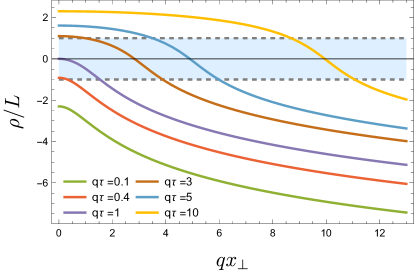
Figure 1: $\rho/L$ plotted as a function of $qx_{\perp}$ for various fixed values of $q\tau$. The gray dashed lines at $-1$ and 1 mark the boundary of the applicability of a hydro-like region (shaded blue).

In order to gain further insight, it is useful to rearrange (28) in a form that readily gives a profile which decays at large $x_{\perp}$ in Minkowski space. Each term in the sum (28), which is of the form $\exp(-(4+2n)\rho/L)$ with $n$ a non-negative integer, grows with $x_{\perp}$ in Minkowski space as $(x_{\perp}^{2}/\tau)^{4+2n}$ at any fixed $\tau>0$. It is easy to see that the following expansion

$$\hat{\varepsilon}(\rho) = \sum_{n=0}^{\infty}\frac{a_{n}}{\cosh^{4+2n}(\rho/L)}$$ (32)

$$+\sum_{n=0}^{\infty}\frac{b_{n}}{(2\cosh(\rho/L)+\sinh(\rho/L))^{4+2n}}$$

is equivalent to the general large $\rho$ expansion (28) for $\rho\gg L$, but with each term that decays along the transverse directions in Minkowski space at any fixed $\tau>0$. (Note ${\rm sech}(\rho/L)$ decays with large $x_{\perp}$ as $x_{\perp}^{-2}$ at any fixed $\tau>0$, etc.) In the second set of terms above, we have used $2\cosh(x)+\sinh(x)$ instead of $\sinh(x)$, since then the denominator does not vanish at any value of $\rho$. Also note that without the second set of terms we get an additional $\rho\rightarrow-\rho$ (de Sitter time-reversal) symmetry which is not a feature of generic Gubser flow.

Clearly, (32) implies that $\hat{\epsilon}(\rho)\sim\exp(4\rho/L)$ gives regular bulk geometry at small $\tau$ (large and negative $\rho$). This needs to be verified explicitly. We note that the exact solutions of the massless scalar field (23) and (24) indeed realize such an early time behavior for the expectation value of the marginal operator which behaves at late time identically as $\hat{\varepsilon}(\rho)$ (see (22)). These solutions are indeed regular for $\tau>0$ (the entire future wedge). Furthermore, (32) is consistent with the hydrodynamic expansion (12) at $\rho=0$, and in fact predicts that $\hat{\varepsilon}$ is just a power series at $\rho=0$ even after including all the other non-hydrodynamic transients. This needs to be explicitly verified as well. With such caveats, we proceed to see what follows from using this general form (32) on the entire future wedge beyond the large $\rho$ domain.

After changing to Minkowski frame using (11), we find that (32) gives the small $\tau$ behavior (with $x=qx_{\perp}$ and $t=q\tau$):

$$\varepsilon(x_{\perp},\tau)=q^{4}L^{4}\Bigg{(}\frac{16(a_{0}+b_{0})}{(x^{2}+1)^{4}}$$

$$+\frac{64(a_{1}+b_{1}+b_{0}(-3+x^{2})+a_{0}(-1+x^{2}))}{(x^{2}+1)^{4}}t^{2}+\mathcal{O}(t^{3})\Bigg{)}.$$ (33)

Remarkably, only $a_{0}$ and $b_{0}$ determine the leading universal form of $\varepsilon$ at $\tau\rightarrow 0$. At the next order ($\tau^{2}$), only the sub-leading terms in (32), namely $a_{1}$ and $b_{1}$, appear, and so on. Thus the late time expansion (28) can be systematically matched with that at early time with the same pair of coefficients appearing in both at each order.

Furthermore, the leading term in (V) implies that, in the limit $\tau\rightarrow 0$, we also obtain $\varepsilon=P_{T}=-P_{L}$ exactly like in the large $\rho$ domain. This matches with the color glass condensate behavior Epelbaum and Gelis (2013); Müller (2019); Berges et al. (2021) expected in the initial stages of actual heavy-ion collision experiments. Irrespectively, such initial conditions are special, and not of the colliding shock wave type studied numerically by Chesler and Yaffe Chesler and Yaffe (2011) where hydrodynamics dominates late time behavior.

It also follows that $\varepsilon$ takes the following general form:

$$\varepsilon(x_{\perp},\tau)=\frac{A}{\left(x^{2}\exp\left(-\sum_{n=1}^{\infty}\frac{\beta_{n}(t)}{x^{4n}}-\sum_{n=0}^{\infty}\frac{\gamma_{n}(t)}{x^{4n+2}}\right)+1\right)^{4}}.$$ (34)

We note that (V) implies that $\beta_{n}(0)=\gamma_{n}(0)=0$. To determine $A$, $\beta_{n}(t)$ and $\gamma_{n}(t)$, we need to compare the large $x_{\perp}$ expansion of (32) obtained after changing to Minkowski frame via (11) with the same expansion of (34). This systematic matching gives

$$A=16(a_{0}+b_{0})q^{4}L^{4},\,\,\gamma_{0}(t)=t^{2},$$

$$\beta_{1}(t)=\frac{t^{2}(2(a_{1}+b_{1})+b_{0}(-8+t^{2})+a_{0}(-4+t^{2}))}{2(a_{0}+b_{0})},\ldots$$ (35)

We find that $\beta_{n}(t)$ and $\gamma_{n}(t)$ are polynomials of $t$ of orders $4n$ and $(4n+2)$, respectively. Thus the behavior of $\varepsilon$ in the large $x_{\perp}$ (peripheral) region ($x_{\perp}\gg\tau$) for any fixed $\tau$ is also determined systematically by (32).

In the future, we plan to find the generic behavior at $\rho=0$, study matching with early and late time while comparing with trans-series discussed in Behtash et al. (2018); Denicol and Noronha (2019); Behtash et al. (2020); Dash and Roy (2020); Soloviev (2022).

VI Discussion

We have provided some exact results on how relativistic quantum matter evolves in Gubser flow in large $N$ holographic strongly coupled conformal field theories. The most generic behaviour is yet to established and further progress can be made by employing numerical relativity in this context.

The main implications of our results for the holographic conformal Gubser flow that, in flows with such special symmetries, a relativistic quantum system can evolve out of hydrodynamics into a new regime that can mirror the initial conditions while finally entering into a novel phase which is universal in the sense that it is independent of the state of the system at early time. Furthermore, such flows require special initial conditions which satisfy more restrictions beyond those implied by the symmetries. Nevertheless, such evolutions, if realized, can reveal many fundamental features of the underlying microscopic theory, and thus further investigations on the Gubser flow are relevant for the phenomenology of the heavy ion collisions and understanding the nature of strong interactions. Therefore, we plan to study Gubser flow in holographic non-conformal/confining gauge theories Gursoy et al. (2016); Chattopadhyay et al. (2022); Jaiswal et al. (2022); Chen and Yan (2022) and in semi-holographic Iancu and Mukhopadhyay (2015); Banerjee et al. (2017); Kurkela et al. (2018); Mitra et al. (2020, 2022) scenarios and see how both, the initial conditions and the late de-Sitter regime for the Gubser flow distinguishes confining behaviour from an emergent infrared critical point. It would be interesting to understand the likelihood of such initial conditions in actual heavy-ion collisions.

The advantage of studying Gubser flow in a holographic theory is that we can understand the quantum information theoretic aspects of such a scenario in which a many-body system can escape hydrodynamization. Many novel aspects of quantum thermodynamics Landi and Paternostro (2021) can be understood via explicit computations of entanglement measures (see for example Kibe et al. (2022); Banerjee et al. (2022)). A preliminary discussion on the entropy production captured by the growth of the area of the horizons, and puzzles regarding its interpretation has been presented in the Supplementary Material.

Appendix A Viscous Hydrodynamics

The conformal viscous Gubser flow has been studied in Gubser and Yarom (2011). The conformal perfect fluid energy-momentum tensor is $\hat{t}^{\mu\nu}_{0}=\varepsilon(T)(4u^{\mu}u^{\nu}+g^{\mu\nu})$, where $\varepsilon(T)\propto T^{4}$ is determined by the equation of state in terms of the temperature $T$. Including the first order viscous correction, we have

$$\hat{t}^{\mu\nu}=\hat{t}^{\mu\nu}_{0}-2\eta(T)\sigma^{\mu\nu},$$ (36)

where $\sigma^{\mu\nu}$ is the shear stress tensor defined as

$$\sigma^{\mu\nu}=\frac{1}{2}\Delta^{\alpha\mu}\Delta^{\beta\nu}\left(\nabla_{\alpha}u_{\beta}+\nabla_{\beta}u_{\alpha}\right)-\frac{1}{3}\nabla_{\lambda}u^{\lambda}\Delta^{\mu\nu},$$ (37)

and $\eta(T)\propto T^{3}$ is the shear viscosity. It is useful to define $H_{0}=\eta(T)\hat{\varepsilon}^{-3/4}(T)$ which is a constant in a conformal field theory and is determined by microscopic dynamics. Above, $\Delta^{\mu\nu}=u^{\mu}u^{\nu}+g^{\mu\nu}$. The conservation of the energy-momentum tensor (i.e. the hydrodynamic equations) for the Gubser flow in ${\rm d}S_{3}\times\mathbf{R}$ frame is simply

$$\hat{\varepsilon}^{\prime}({\tilde{\rho}})+\frac{8}{3}\tanh({\tilde{\rho}})\hat{\varepsilon}({\tilde{\rho}})-\frac{16}{9}H_{0}\tanh^{2}({\tilde{\rho}})\hat{\varepsilon}({\tilde{\rho}})^{3/4}=0,$$ (38)

with ${\tilde{\rho}}=\rho/L$. The solution of this equation is

$$\varepsilon({\tilde{\rho}}) =\frac{\text{sech}^{4}({\tilde{\rho}})}{531441}\Big{(}4H_{0}L^{-1}\sinh^{3}({\tilde{\rho}}){\cosh^{1/3}({\tilde{\rho}})}$$

$${}_{2}F_{1}\left(\frac{7}{6},\frac{3}{2};\frac{5}{2};-\sinh^{2}({\tilde{\rho}})\right)+27\hat{\varepsilon}_{0}^{1/4}{\cosh^{1/3}({\tilde{\rho}})}\Big{)}{}^{4}.$$ (39)

The viscous energy density $\hat{\varepsilon}$ in the limit ${\tilde{\rho}}\rightarrow 0$ gives the derivative expansion (12) as mentioned in the main text. However, in the limit ${\tilde{\rho}}\rightarrow\infty$ the energy density has the following expansion dominated by viscous term at the leading order:

$$\hat{\varepsilon}({\tilde{\rho}})=\frac{16}{81}H_{0}^{4}L^{-4}+\mathcal{O}(\cosh({\tilde{\rho}})^{-2/3})+\ldots$$ (40)

This indicates the breakdown of derivative expansion in the large ${\tilde{\rho}}$ limit.

Appendix B Holographic renormalization

For compactness, we define ${\tilde{\rho}}=\rho/L$ and also use the variable $v$ with $v=r/L$ as in the main text. We can solve for the metric functions $A(v,{\tilde{\rho}}),B(v,{\tilde{\rho}})$ and $C(v,{\tilde{\rho}})$ in the radial expansion near the boundary $v=0$ as indicated in (III) and obtain,

$$A(v,{\tilde{\rho}})=a_{(1)}\left({\tilde{\rho}}\right)v+\frac{1}{4}\left(a_{(1)}^{2}\left({\tilde{\rho}}\right)-4a_{(1)}^{\prime}\left({\tilde{\rho}}\right)\right)v^{2}$$

$$+a_{(4)}\left({\tilde{\rho}}\right)v^{4}+\ldots,$$ (41)

$$B(v,{\tilde{\rho}})=a_{(1)}({\tilde{\rho}})\cosh^{2}({\tilde{\rho}})~{}v$$

$$-\frac{1}{4}a_{(1)}({\tilde{\rho}})\left(a_{(1)}({\tilde{\rho}})+4\tanh({\tilde{\rho}})\right)~{}v^{2}$$

$$+\frac{1}{12}a_{(1)}({\tilde{\rho}})\Big{(}\left(a_{(1)}({\tilde{\rho}})+3\tanh\left({\tilde{\rho}}\right)\right)^{2}+3\tanh^{2}\left({\tilde{\rho}}\right)\Big{)}~{}v^{3}$$

$$+b_{(4)}({\tilde{\rho}})~{}v^{4}+\ldots,$$ (42)

$$C(v,{\tilde{\rho}})=3a_{(1)}({\tilde{\rho}})~{}v-\frac{1}{4}a_{(1)}({\tilde{\rho}})\Big{(}8\tanh({\tilde{\rho}})+3a_{(1)}({\tilde{\rho}})\Big{)}~{}v^{2}$$

$$+\frac{1}{4}a_{(1)}({\tilde{\rho}})\left(\left(a_{(1)}({\tilde{\rho}})+2\tanh({\tilde{\rho}})\right)^{2}+4\tanh^{2}({\tilde{\rho}})\right)~{}v^{3}$$

$$+s_{(4)}({\tilde{\rho}})~{}v^{4}+\ldots,$$ (43)

where $a_{(1)}\left({\tilde{\rho}}\right)$ is an arbitrary function. The functions $b_{(4)}\left({\tilde{\rho}}\right)$ and $s_{(4)}\left({\tilde{\rho}}\right)$ are determined by $a_{(4)}\left({\tilde{\rho}}\right)$ and $a_{(1)}\left({\tilde{\rho}}\right)$ by the constraints of Einstein’s equations:

$$s_{(4)}\left({\tilde{\rho}}\right)=-\frac{1}{32}a_{(1)}\left({\tilde{\rho}}\right)\Big{(}a_{(1)}^{2}\left({\tilde{\rho}}\right)+4\tanh^{2}\left({\tilde{\rho}}\right)\Big{)}$$

$$\Big{(}3a_{(1)}\left({\tilde{\rho}}\right)+16\tanh\left({\tilde{\rho}}\right)\Big{)}+\frac{9}{8}a_{(1)}^{2}\left({\tilde{\rho}}\right)\tanh^{2}\left({\tilde{\rho}}\right),$$

$$a_{(4)}^{\prime}\left({\tilde{\rho}}\right)=\frac{8}{3}\tanh\left({\tilde{\rho}}\right)\Big{(}b_{(4)}\left({\tilde{\rho}}\right)-a_{(4)}\left({\tilde{\rho}}\right)\Big{)}$$

$$+\frac{1}{12}\Big{(}a_{(1)}^{3}\left({\tilde{\rho}}\right)+4a_{(1)}\left({\tilde{\rho}}\right)\tanh^{2}\left(\frac{\rho}{L}\right)\Big{)}$$

$$\Big{(}a_{(1)}\left({\tilde{\rho}}\right)+8\tanh\left({\tilde{\rho}}\right)\Big{)}+\frac{5}{6}a_{(1)}^{2}\left({\tilde{\rho}}\right)\tanh^{2}\left({\tilde{\rho}}\right).$$ (44)

We find that the radial expansions and thus $A$, $B$ and $C$ are entirely determined by the two functions $a_{(4)}\left({\tilde{\rho}}\right)$ and $a_{(1)}\left({\tilde{\rho}}\right)$.

However, $a_{(1)}\left({\tilde{\rho}}\right)$ is a residual gauge freedom and can be set to zero by the diffeomorphism $v\rightarrow v+f({\tilde{\rho}})$ which preserves the ingoing Eddington-Finkelstein gauge. Furthermore, the latter is a proper diffeomorphism, meaning that $a_{(1)}\left({\tilde{\rho}}\right)$ does not affect boundary data. Indeed extracting the dual energy-momentum tensor $\langle T^{\mu}_{\,\nu}\rangle$ at the boundary from the renormalized on-shell gravitational action following Henningson and Skenderis (1998); Balasubramanian and Kraus (1999); de Haro et al. (2001) and using (B), we find that $a_{(1)}\left({\tilde{\rho}}\right)$ disappears. Explicitly, we obtain

$$\langle T^{\mu}_{\,\nu}\rangle=\begin{pmatrix}\hat{t}^{\rho}_{\,\rho}&0&0&0\\ 0&\hat{t}^{\theta}_{\,\theta}&0&0\\ 0&0&\hat{t}^{\phi}_{\,\phi}&0\\ 0&0&0&\hat{t}^{\eta}_{\,\eta}\end{pmatrix}+\mathcal{A}^{\mu}_{\,\nu}$$ (45)

where

$$\hat{t}^{\rho}_{\,\rho}\equiv-\hat{\varepsilon}\left({\tilde{\rho}}\right)=\frac{3l^{3}}{16\pi G_{N}}a_{(4)}\left({\tilde{\rho}}\right),$$

$$\hat{t}^{\theta}_{\,\theta}\equiv\hat{P_{T}}\left({\tilde{\rho}}\right)=\frac{3l^{3}}{16\pi G_{N}}\left(\frac{1}{2}\coth\left({\tilde{\rho}}\right)a_{(4)}^{\prime}\left({\tilde{\rho}}\right)+a_{(4)}\left({\tilde{\rho}}\right)\right),$$

$$\hat{t}^{\phi}_{\,\phi}\equiv\hat{P_{T}}\left({\tilde{\rho}}\right)=\hat{t}^{\theta}_{\,\theta},$$

$$\hat{t}^{\eta}_{\,\eta}\equiv\hat{P_{L}}\left({\tilde{\rho}}\right)=-\frac{3l^{3}}{16\pi G_{N}}\Big{(}\coth\left({\tilde{\rho}}\right)a_{(4)}^{\prime}\left({\tilde{\rho}}\right)+3a_{(4)}\left({\tilde{\rho}}\right)\Big{)}.$$ (46)

and $\mathcal{A}^{\mu}_{\,\nu}$ is the Weyl anomaly given by

$$\hat{\mathcal{A}}^{\mu}_{\,\nu} = \frac{l^{3}}{128\pi G_{N}}\Big{(}\frac{4}{3}R^{\mu}_{\,\nu}R-2R^{\mu}_{\,\kappa}R^{\kappa}_{\,\nu}-\delta^{\mu}_{\,\nu}\Big{(}\frac{1}{2}R^{2}-R_{\kappa\sigma}R^{\kappa\sigma}\Big{)}\Big{)}$$ (47)

$$= \frac{l^{3}}{64\pi G_{N}}diag\left(1,1,1,-3\right)L^{-4},$$

where the curvatures refer to those of the background metric (4) for the dual theory (which is also the boundary metric of the five-dimensional bulk spacetime). With the identification $l^{3}/G_{N}=2N^{2}/\pi$, we obtain (10).

Appendix C Finding values of $\alpha$ for pure gravity

Here we give details of how $\alpha$ has been determined replicating the strategy for the massless scalar field discussed in the main text. The ansatz (25) is a double expansion in $\sigma$. Assuming analytic behavior at the future horizon $r=L$ (i.e. $v=1$), we obtain the near horizon expansion (with numerical coefficients $a_{nm,p}$)

$$A_{nm}(v)=\sum_{p=0}^{\infty}a_{nm,p}(1-v)^{p},$$ (48)

and similarly for $B_{nm}(v)$ and $C_{nm}(v)$ in terms of the numerical coefficients $b_{nm,p}$ and $c_{nm,p}$, respectively. Solving the gravitational equations in this near-horizon expansion, we find that $A_{10}(v)$, $B_{10}(v)$ and $C_{10}(v)$ are determined by the three integration constants $a_{10,0}$, $b_{10,0}$ and $c_{10,0}$. Explicitly,

$$A_{10}(v)=a_{10,0}\left(1-(\alpha+1)(1-v)+\mathcal{O}((1-v)^{2})\ldots\right)$$

$$+b_{10,0}\left(-2\alpha(1-v)+\mathcal{O}((1-v)^{2})+\ldots\right)$$

$$+c_{10,0}\left(\frac{1}{2}\alpha(1+\alpha)(1-v)+\mathcal{O}((1-v)^{2})+\ldots\right),$$ (49)

and also similarly for $B_{10}(v)$ and $C_{10}(v)$.

Normalizable solutions can be matched to the near-boundary expansion (B)-(B). However, the solution of $A_{10}(v)$ given by (C) when expanded near the boundary $v=0$ reads as

$$A_{10}(v) =P(\alpha)(a_{10,0}+(1+\alpha)(2b_{10,0}-c_{10,0}))$$ (50)

$$+\mathcal{O}(v)+\ldots$$

where $P(\alpha)$ is polynomial in $\alpha$. Therefore, for normalizability, $\alpha$ should be the roots of $P(\alpha)$ and these are $\alpha=2k$, with $k=0,1,2,\ldots$. This can be found by performing the expansion (C) to high orders and then re-expanding it as a Taylor series about $v=0$ as in the case of the massless scalar.

For $k=0$, $A_{10}$, $B_{10}$ and $C_{10}$ vanish. For the case $k=1$ we have been able to find a solution which corresponds to the boundary expansion (B)-(B) with $a_{(1)}({\tilde{\rho}})\neq 0$ but $a_{(4)}({\tilde{\rho}})=0$. Since $a_{(1)}({\tilde{\rho}})$ corresponds to a pure residual (proper) gauge freedom, this solution for the case $k=1$ yields just a pure gauge deformation. However, we cannot rule out this case completely as another physical solution may exist. For $k=2,3,\ldots$, we are able to find physical solutions as reported in the main text.

To see how we reach these conclusions, it is useful to use the residual gauge freedom to set $a_{(1)}({\tilde{\rho}})=0$. In this case, the near boundary expansions (B)-(B) start from $v^{4}$. For the comparison with near-horizon expansions for $A_{10}$, $B_{10}$ and $C_{10}$ we should further impose a late-time expansion of $a_{4}({\tilde{\rho}})$ of the form

$$a_{(4)}({\tilde{\rho}})=\sum_{n=1}^{\infty}\sum_{m=0}^{\infty}\sigma^{-n\alpha-2m}a_{(4)nm}$$ (51)

that follows from (25) with constant coefficients $a_{(4)nm}$. Setting the coefficients of $v$ and $v^{2}$ to zero in (50), we get two relations between the three integration constants $a_{10,0}$, $b_{10,0}$ and $c_{10,0}$. For $k=0$, these simply set $a_{10.0}=0$ and then requiring that the boundary values of $B_{10}$ and $C_{10}$ to vanish (so that we get normalizable solutions) we obtain $b_{10.0}=c_{10.0}=0$. Then $A_{10}$, $B_{10}$ and $C_{10}$ have to vanish. For $k\geq 2$, setting the coefficients of $v$ and $v^{2}$ to zero in (50) give two relations to determine $b_{10,0}$ and $c_{10,0}$ in terms of $a_{10,0}$. Using these values of $b_{10,0}$ and $c_{10,0}$, we find a perfect agreement with the near boundary expansions (B)-(B) corresponding to normalizable solutions where the residual gauge freedom has been fixed with $a_{(1)}=0$. The remaining integration constant $a_{10,0}$ simply determines the leading term in $a_{(4)}({\tilde{\rho}})$ in (51), i.e. $a_{(4)10}$. For the allowed values of $\alpha$ which are $4+2n$, with $n=0,1,2,\ldots$ the ansatz (25) can be simplified to (27), as mentioned before. (Then $a_{(4)10}$ identified with $\hat{e}_{0}$ up to a numerical constant, etc.) The case $k=1$ is somewhat tricky because the series expansion of the equations near the horizon themselves do not have unique solutions. One way of solving it leads to a pure gauge solution. We have not been able to show that physical solutions do not exist for this case.

At higher orders in the late de-Sitter time expansion in case of $\alpha=4+2n$ and $n=0,1,2,\ldots$, we obtain normalizable solutions because the lower orders source only normalizable particular solutions, while the homogeneous solutions are also normalizable with a new arbitrary integration constant at each order since $\alpha=6,8,\ldots$ are allowed to be the leading order behavior also (when the lower order coefficients vanish). This argument is similar to the case of the massless bulk scalar. We thus establish that (28) gives realizable late de Sitter time expansion for the dual energy density.

Appendix D Examining the entropy

Let us first examine the entropy $S$ in the de Sitter frame. The entropy $S$ of the black hole given by (III) is given by the area $\Sigma_{H}$ of the apparent or event horizon located at $v=v_{h}({\tilde{\rho}})$

$$S=\frac{\Sigma_{H}}{4G_{N}}$$ (52)

where $G_{N}$ is the Newton constant. Here we will examine the event horizon. The area can be computed via $\Sigma_{H}=\int_{v=v_{h}}\sqrt{\gamma}~{}d\theta~{}d\phi~{}d\eta$ with $\gamma$ being the induced metric on the spatial sections of the event horizon (generated by a congruence of null geodesics). Explicitly,

$$\gamma=l^{6}\frac{e^{C(v_{h}({\tilde{\rho}}),{\tilde{\rho}})}\sin^{2}\theta\left(\cosh\left({\tilde{\rho}}\right)+v_{h}({\tilde{\rho}})\sinh\left({\tilde{\rho}}\right)\right)^{4}}{v_{h}^{6}({\tilde{\rho}})}.$$ (53)

Here $\theta\in[0,\pi]$, $\phi\in[0,2\pi]$ and $\eta\in[-\infty,\infty]$. Due to the infinite extent of $\eta$, it is better to define the entropy per unit rapidity which is

$$\frac{dS}{d\eta}=\pi\frac{l^{3}}{G_{N}}\frac{e^{\frac{C(v_{h}({\tilde{\rho}}),{\tilde{\rho}})}{2}}\left(\cosh\left({\tilde{\rho}}\right)+v_{h}({\tilde{\rho}})\sinh\left({\tilde{\rho}}\right)\right)^{2}}{v_{h}^{3}({\tilde{\rho}})}.$$ (54)

The corresponding entropy density per unit rapidity reads

$$\frac{ds}{d\eta}=\frac{1}{4\pi L^{3}\cosh^{2}\left({\tilde{\rho}}\right)}\frac{dS}{d\eta}.$$ (55)

The factor of $4\pi\cosh^{2}\left({\tilde{\rho}}\right)$ is the area of the sphere at the boundary (measured by the background metric (4)). The location of the event horizon $v_{h}({\tilde{\rho}})$ can be determined by the radial null geodesic equation, i.e.

$$\frac{{\rm d}v_{h}({\tilde{\rho}})}{{\rm d}{\tilde{\rho}}}+\frac{1-v_{h}^{2}({\tilde{\rho}})+A(v_{h}({\tilde{\rho}}),{\tilde{\rho}})}{2}=0$$ (56)

with the condition that $v_{h}({\tilde{\rho}}=\infty)=1$, since the horizon coincides with that of the solution dual to the vacuum in the limit ${\tilde{\rho}}\rightarrow\infty$.

In the state dual to the vacuum, we simply have

$$\frac{ds}{d\eta}=\frac{l^{3}}{4L^{3}\cosh^{2}\left({\tilde{\rho}}\right)G_{N}}\left(\cosh\left({\tilde{\rho}}\right)+\sinh\left({\tilde{\rho}}\right)\right)^{2},$$

$$=\frac{l^{3}}{L^{3}G_{N}}\times\frac{1}{4}\left(1+\tanh\left({\tilde{\rho}}\right)\right)^{2}.$$ (57)

This implies that the entropy density per unit rapidity monotonically increases from zero to a constant value with the de Sitter time as shown in Fig. 2.

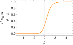
Figure 2: Vacuum entropy density per unit rapidity plotted as a function of ${\tilde{\rho}}$. The figure shows that at late-time $ds/d\eta$ goes to a constant.

At this point, it would seem strange to associate an entropy to the vacuum state in the Gubser flow. However, this is the entropy associated with an accelerated observer, since the de Sitter frame is accelerating from the Minkowski point of view (like the Rindler observer is accelerating and one can also associate an entropy with such an observer). Since, the de Sitter frame is the co-moving frame for the flow, it is natural to associate an entropy with such a frame. In the bulk, this entropy is realized via the bulk diffeomorphism which implements the necessary Weyl transformation (4) at the boundary. (A bulk diffeomorphism can produce a non-trivial entropy as in the case of the map from pure three-dimensional anti-de Sitter space ($AdS_{3}$) to the Banados Teitelboim Zanelli (BTZ) black hole Banados et al. (1992), however the physical interpretation of the entropy in our case is more similar to that in Emparan (1999).)

The bulk dual of aGubser flow admits the late-time expansion (27), and thus the location of the event horizon which is a solution of (56) with the condition $v_{h}({\tilde{\rho}}=\infty)=1$, admits the following expansion

$$v_{h}({\tilde{\rho}})=1+\sum_{m=0}^{\infty}v_{h,m}e^{-(4+2m){\tilde{\rho}}}$$ (58)

at late time. Using the explicit perturbative solution for the metric given by (29)-(31), we obtain

$$v_{h,0}=\frac{\hat{e}_{0}}{40},\quad v_{h,1}=\frac{24\hat{e}_{0}+29\hat{e}_{1}}{2240},\quad\ldots$$ (59)

and

$$L^{3}\frac{G_{N}}{l^{3}}\frac{ds}{d\eta}=1-2e^{-2{\tilde{\rho}}}+3\left(1-\frac{\hat{e}_{0}}{80}\right)e^{-4{\tilde{\rho}}}+\ldots$$ (60)

In the case of the vacuum with $0=\hat{e}_{0}=\ldots$, the above series has alternating signs. However, the function is monotonically increasing (and assuming the value $1$ in the limit ${\tilde{\rho}}\rightarrow\infty$) as evident from the exact expression (D) (that is plotted in Fig. 2). The monotonic growth of the entropy density per unit rapidity is not affected perturbatively and it reaches the constant vacuum value at late time. It has been shown in Maldacena and Pimentel (2013) that the entanglement entropy can scale as the volume in de Sitter space with a numerical factor which has a maximal value. If $\hat{e}_{0}$ is positive, then the energy density at leading order is negative, and $ds/d\eta$ is less than in the vacuum. On the other hand if $\hat{e}_{0}$ is negative, then the energy density at leading order is positive, and $ds/d\eta$ is larger than that in the vacuum. Here, it is also useful to note that it has been argued that the entropy of an excited state in de Sitter space is expected to be less than that of the vacuum Chandrasekaran et al. (2023). It will be useful to understand the case of the holographic Gubser flow better with a clear algebraic interpretation of $ds/d\eta$ computed here.

References

- Gubser (2010) S. S. Gubser, Phys. Rev. D 82, 085027 (2010), arXiv:1006.0006 [hep-th] .
- Gubser and Yarom (2011) S. S. Gubser and A. Yarom, Nucl. Phys. B 846, 469 (2011), arXiv:1012.1314 [hep-th] .
- Denicol et al. (2014a) G. S. Denicol, U. W. Heinz, M. Martinez, J. Noronha, and M. Strickland, Phys. Rev. Lett. 113, 202301 (2014a), arXiv:1408.5646 [hep-ph] .
- Denicol et al. (2014b) G. S. Denicol, U. W. Heinz, M. Martinez, J. Noronha, and M. Strickland, Phys. Rev. D 90, 125026 (2014b), arXiv:1408.7048 [hep-ph] .
- Denicol and Noronha (2019) G. S. Denicol and J. Noronha, Phys. Rev. D 99, 116004 (2019), arXiv:1804.04771 [nucl-th] .
- Chattopadhyay et al. (2019) C. Chattopadhyay, U. Heinz, S. Pal, and G. Vujanovic, Nucl. Phys. A 982, 287 (2019), arXiv:1807.05462 [nucl-th] .
- Behtash et al. (2020) A. Behtash, S. Kamata, M. Martinez, and H. Shi, JHEP 07, 226 (2020), arXiv:1911.06406 [hep-th] .
- Dash and Roy (2020) A. Dash and V. Roy, Phys. Lett. B 806, 135481 (2020), arXiv:2001.10756 [nucl-th] .
- Berger (2002) B. K. Berger, Living Rev. Rel. 5, 1 (2002), arXiv:gr-qc/0201056 .
- Epelbaum and Gelis (2013) T. Epelbaum and F. Gelis, Phys. Rev. Lett. 111, 232301 (2013), arXiv:1307.2214 [hep-ph] .
- Müller (2019) D. Müller, Simulations of the Glasma in 3+1D, Ph.D. thesis, Vienna, Tech. U. (2019), arXiv:1904.04267 [hep-ph] .
- Berges et al. (2021) J. Berges, M. P. Heller, A. Mazeliauskas, and R. Venugopalan, Rev. Mod. Phys. 93, 035003 (2021), arXiv:2005.12299 [hep-th] .
- Henningson and Skenderis (1998) M. Henningson and K. Skenderis, JHEP 07, 023 (1998), arXiv:hep-th/9806087 .
- Balasubramanian and Kraus (1999) V. Balasubramanian and P. Kraus, Commun. Math. Phys. 208, 413 (1999), arXiv:hep-th/9902121 .
- Maldacena (1998) J. M. Maldacena, Adv. Theor. Math. Phys. 2, 231 (1998), arXiv:hep-th/9711200 .
- Witten (1998) E. Witten, Adv. Theor. Math. Phys. 2, 253 (1998), arXiv:hep-th/9802150 .
- Gubser et al. (1998) S. S. Gubser, I. R. Klebanov, and A. M. Polyakov, Phys. Lett. B 428, 105 (1998), arXiv:hep-th/9802109 .
- Freedman et al. (1999) D. Z. Freedman, S. S. Gubser, K. Pilch, and N. P. Warner, Adv. Theor. Math. Phys. 3, 363 (1999), arXiv:hep-th/9904017 .
- Heemskerk and Polchinski (2011) I. Heemskerk and J. Polchinski, JHEP 06, 031 (2011), arXiv:1010.1264 [hep-th] .
- Bredberg et al. (2011) I. Bredberg, C. Keeler, V. Lysov, and A. Strominger, JHEP 03, 141 (2011), arXiv:1006.1902 [hep-th] .
- Kuperstein and Mukhopadhyay (2011) S. Kuperstein and A. Mukhopadhyay, JHEP 11, 130 (2011), arXiv:1105.4530 [hep-th] .
- Kuperstein and Mukhopadhyay (2013) S. Kuperstein and A. Mukhopadhyay, JHEP 11, 086 (2013), arXiv:1307.1367 [hep-th] .
- Behr and Mukhopadhyay (2016) N. Behr and A. Mukhopadhyay, Phys. Rev. D 94, 026002 (2016), arXiv:1512.09055 [hep-th] .
- Behr et al. (2016) N. Behr, S. Kuperstein, and A. Mukhopadhyay, Phys. Rev. D 94, 026001 (2016), arXiv:1502.06619 [hep-th] .
- Mukhopadhyay (2016) A. Mukhopadhyay, Int. J. Mod. Phys. A 31, 1630059 (2016), arXiv:1612.00141 [hep-th] .
- de Haro et al. (2001) S. de Haro, S. N. Solodukhin, and K. Skenderis, Commun. Math. Phys. 217, 595 (2001), arXiv:hep-th/0002230 .
- Skenderis (2002) K. Skenderis, Class. Quant. Grav. 19, 5849 (2002), arXiv:hep-th/0209067 .
- Rangamani (2009) M. Rangamani, Class. Quant. Grav. 26, 224003 (2009), arXiv:0905.4352 [hep-th] .
- Gupta and Mukhopadhyay (2009) R. K. Gupta and A. Mukhopadhyay, JHEP 03, 067 (2009), arXiv:0810.4851 [hep-th] .
- Chesler and Yaffe (2011) P. M. Chesler and L. G. Yaffe, Phys. Rev. Lett. 106, 021601 (2011), arXiv:1011.3562 [hep-th] .
- Behtash et al. (2018) A. Behtash, C. N. Cruz-Camacho, and M. Martinez, Phys. Rev. D 97, 044041 (2018), arXiv:1711.01745 [hep-th] .
- Soloviev (2022) A. Soloviev, Eur. Phys. J. C 82, 319 (2022), arXiv:2109.15081 [hep-th] .
- Gursoy et al. (2016) U. Gursoy, M. Jarvinen, and G. Policastro, JHEP 01, 134 (2016), arXiv:1507.08628 [hep-th] .
- Chattopadhyay et al. (2022) C. Chattopadhyay, S. Jaiswal, L. Du, U. Heinz, and S. Pal, Phys. Lett. B 824, 136820 (2022), arXiv:2107.05500 [nucl-th] .
- Jaiswal et al. (2022) S. Jaiswal, C. Chattopadhyay, L. Du, U. Heinz, and S. Pal, Phys. Rev. C 105, 024911 (2022), arXiv:2107.10248 [hep-ph] .
- Chen and Yan (2022) Z. Chen and L. Yan, Phys. Rev. C 105, 024910 (2022), arXiv:2109.06658 [nucl-th] .
- Iancu and Mukhopadhyay (2015) E. Iancu and A. Mukhopadhyay, JHEP 06, 003 (2015), arXiv:1410.6448 [hep-th] .
- Banerjee et al. (2017) S. Banerjee, N. Gaddam, and A. Mukhopadhyay, Phys. Rev. D 95, 066017 (2017), arXiv:1701.01229 [hep-th] .
- Kurkela et al. (2018) A. Kurkela, A. Mukhopadhyay, F. Preis, A. Rebhan, and A. Soloviev, JHEP 08, 054 (2018), arXiv:1805.05213 [hep-ph] .
- Mitra et al. (2020) T. Mitra, S. Mondkar, A. Mukhopadhyay, A. Rebhan, and A. Soloviev, Phys. Rev. Res. 2, 043320 (2020), arXiv:2006.09383 [hep-ph] .
- Mitra et al. (2022) T. Mitra, S. Mondkar, A. Mukhopadhyay, A. Rebhan, and A. Soloviev, (2022), arXiv:2211.05480 [hep-ph] .
- Landi and Paternostro (2021) G. T. Landi and M. Paternostro, Rev. Mod. Phys. 93, 035008 (2021).
- Kibe et al. (2022) T. Kibe, A. Mukhopadhyay, and P. Roy, Phys. Rev. Lett. 128, 191602 (2022), arXiv:2109.09914 [hep-th] .
- Banerjee et al. (2022) A. Banerjee, T. Kibe, N. Mittal, A. Mukhopadhyay, and P. Roy, Phys. Rev. Lett. 129, 191601 (2022), arXiv:2202.00022 [hep-th] .
- Banados et al. (1992) M. Banados, C. Teitelboim, and J. Zanelli, Phys. Rev. Lett. 69, 1849 (1992), arXiv:hep-th/9204099 .
- Emparan (1999) R. Emparan, JHEP 06, 036 (1999), arXiv:hep-th/9906040 .
- Maldacena and Pimentel (2013) J. Maldacena and G. L. Pimentel, JHEP 02, 038 (2013), arXiv:1210.7244 [hep-th] .
- Chandrasekaran et al. (2023) V. Chandrasekaran, R. Longo, G. Penington, and E. Witten, JHEP 02, 082 (2023), arXiv:2206.10780 [hep-th] .