Alleviating the quantum Big- problem
Abstract
A major obstacle for quantum optimizers is the reformulation of constraints as a quadratic unconstrained binary optimization (QUBO). Current QUBO translators exaggerate the weight of the penalty terms. Classically known as the “Big-” problem, the issue becomes even more daunting for quantum solvers, since it affects the physical energy scale. We take a systematic, encompassing look at the quantum big- problem, revealing NP-hardness in finding the optimal and establishing bounds on the Hamiltonian spectral gap , inversely related to the expected run-time of quantum solvers. We propose a practical translation algorithm, based on SDP relaxation, that outperforms previous methods in numerical benchmarks. Our algorithm gives values of orders of magnitude greater, e.g. for portfolio optimization instances. Solving such instances with an adiabatic algorithm on 6-qubits of an IonQ device, we observe significant advantages in time to solution and average solution quality. Our findings are relevant to quantum and quantum-inspired solvers alike.
Quantum computing holds a great potential for speeding up combinatorial optimization [1]. From a distant-future perspective, the prospects are rooted in the fact that fault-tolerant quantum computers are envisioned to run quantum versions of state-of-the-art classical optimization algorithms more efficiently. In fact, there is sound theoretical evidence that such quantum algorithms offer a quadratic asymptotic speed-up over their classical counterparts [2, 3, 4]. In the short run, there is a direct relation between the ground state of physical systems and optimizations. The paradigmatic example is Ising models encoding quadratic unconstrained binary optimization (QUBO) problems. This has fueled a quest for ground-state preparation algorithms implementable on nearer-term quantum hardware. These include quantum annealing [5, 6, 7], quantum imaginary time evolution [8, 9, 10, 11, 12, 13, 14], and heuristics such as the quantum approximate optimization algorithm [15, 16, 17]. Moreover, apart from quantum solvers, the QUBO paradigm is giving rise to a variety of interesting quantum-inspired solvers as well [18, 19, 20].
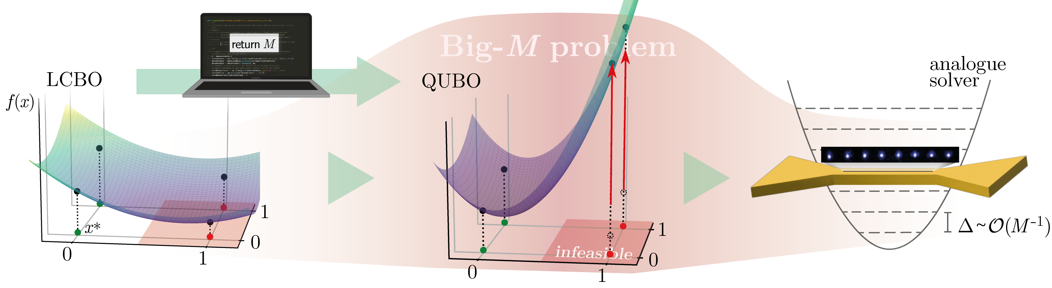
A prerequisite to apply such paradigm to more general quadratically constrained integer optimization problems is to recast them into an equivalent QUBO form. Recently, automatic QUBO translators have appeared [21, 22, 23]. The translation consists of lifting the constraints to penalty terms in the objective function. To ensure that the solution to the reformulated (unconstrained) problem coincides with that of the original (constrained) one, the weight of the penalty terms—often denoted as —has to be sufficiently large. At the same time, choosing an excessively large causes an increase in run-time due to precision issues in rounding and truncation, even for classical solvers. In the classical optimization community this problem is referred to as the Big- problem.
In contrast, quantum QUBO solvers are closer in spirit to analog computing devices. There, the value of directly affects the physical energy scale of the Hamiltonian whose ground state encodes the solution. Ground-state preparation schemes for physical systems are severely restricted by such scale [24, 25, 26]. More precisely, the penalty terms tend to have the undesired side effect of decreasing the spectral gap of the Hamiltonian. As a consequence, the precision required to resolve the states, and, hence, also the run-time, increases. A general rule of thumb is to choose as small as possible, while still successfully enforcing the constraints is highly non-trivial. In fact, the known computationally-efficient Big- recipes tend to largely over-estimate the required value [25, 27, 21]. Clearly, an efficient QUBO translator with improved spectral properties is highly desirable. Moreover, a formalization of the quantum big-M problem as a fundamental concept between quantum physics and computer science is missing too. A general framework should address key aspects such as how to quantify the Big- problem in terms of its impact on quantum solvers or the computational complexity of QUBO reformulations.
Here, we fill in this gap. We develop a theory of the quantum big-M problem and its impact on the spectral gap . We start with rigorous definitions for the notions of optimal and exact QUBO reformulations. We prove that finding the optimal is NP-hard and establish relevant upper bounds on the Hamiltonian spectral gap , both in terms of the original gap and of . One of these bounds formalizes the intuition that . Most importantly, we present a universal QUBO reformulation method with improved spectral properties. This is a simple but remarkably-powerful heuristic recipe for , based on standard SDP relaxation [28]. We perform exhaustive numerical tests on sparse linearly constrained binary optimizations, set partition problems, and portfolio optimizations from real S&P 500 data. For all three classes, we systematically obtain values of one order of magnitude smaller and of from one to two orders of magnitude larger than with state-of-the-art methods, with particularly promising results for portfolio optimization. In addition, in a proof-of-principle experiment, we solved 6-qubit PO instances with a Trotterized adiabatic algorithm deployed on IonQ’s trapped-ion device Aria-1. For the small system size one remains approximately adiabatic with the permissible circuit depth. We observed that our reformulation increases the probability of measuring the optimal solution by over an order of magnitude and improves the average approximation ratio. Our findings demonstrate crucial advantages of the proposed optimized QUBO reformulation over the currently known recipes.
The quantum Big- problem—.
Our starting point is a linearly-constrained binary quadratic optimization (LCBO) problem with binary decision variables and constraints,
| (1) |
specified in terms of , , and . Note that a general polynomially-constrained polynomial optimization problem with integer variables can always be cast into a linearly-constrained binary quadratic optimization problem of the form (1) by standard gadgets, as summarized in App. A. Furthermore, for the sake of clarity, we consider throughout exact optimization solvers. Clearly, near-term quantum optimization solvers are envisioned to be approximate solvers. However, our discussion can be extended to approximate solvers too, e.g. by considering all admissible approximate solutions as optimal points of problem (1).
To arrive at a QUBO formulation of (1), the best-known strategy (see Fig. 1) is to promote the constraints to a quadratic penalty term in the objective function using a suitable constant weight . The resulting QUBO reads,
| (2) |
We say that (2) is an exact reformulation of (1) if their optimal points coincide. The penalty term in (2) vanishes for every feasible point. To arrive at an exact reformulation, has to be chosen large enough for every unfeasible point of (1) to have a greater objective value than the original optimum. Denoting by an optimal point of (1), we have an exact reformulation if and only if there exists a gap s.t.
| (3) |
for all unfeasible points . There are simple choices of to ensure this condition, such as
| (4) |
with the vector -norm being the sum of all absolute entries. Since can be computed in polynomial time, it follows that (1) and (2) with are in the same complexity class. This choice of is common [25, 27, 21]; but, as we show below, it typically yields excessively large values.
We say that a reformulation (2) of (1) has a (-)optimal if it is exact with gap and minimal . Note that the minimal choice of guarantees only a difference between the optimal objective value and those of the unfeasible points. To avoid an arbitrarily small gap, can be chosen as a constant independent on the system size in Eq. (3). For specific classes of problems it is in fact possible to formulate strategies for optimal choices of , an example being the problem of finding maximum independent sets, where the optimal value of is apparent [29]. In general, however, this is intractable.
Observation 1:
Finding an optimal is NP-hard.
Intuitively, Eq. (3) already hints at the possibility that finding the optimal can be as hard as determining the optimal objective value of the original optimization problem. In App. B, we give a polynomial reduction of the problem of deciding if the optimum of is below a threshold to the problem of deciding if a given provides an exact reformulation.
From a pragmatic point of view though, it is nonetheless of utmost importance to find suboptimal but ‘good’ choices of using less resources than required for solving the original problem. In some specific cases (Travelling Salesman Problem [30], permutation problems [31], e.g.), there are recipes for a ‘reasonable’ value for . Here, we provide a generally applicable strategy to determine ‘good’ choices of . At the heart of our approach is the following observation.
Observation 2:
Proof.
Let be an unfeasible point and chosen according to Eq. (5). Since , . The second inequality follows from the definition of and the fact that for any feasible point . Thus, Eq. (3) holds.
While any choice of feasible point and lower bound yields an admissible value of , good choices of attempt to choose the with small objective and the bound as tight as possible. A universal strategy to this end is the following: i) Find a feasible point , by running a classical solver on (1) limited to some constant amount of time. ii) Solve the Semi-definite Programming (SDP) relaxation (see App. E) of the unconstrained minimization of . Use the resulting objective value as . This strategy is our main numerical tool. We denote the value given by it as .
We note that there exist problem instances where even finding a feasible point is hard. In practice, however, there exist efficient heuristics to determine feasible points. The underlying mindset of our strategy is that modern classical solvers can be powerful allies to quantum optimizers, e.g. performing tractable pre-computations to optimize the reformulation for the quantum hardware. As for concluding potential advantages of quantum solvers over classical solvers, with this strategy, one must of course be particularly careful not to accidentally reduce the complexity of the problem in the pre-computation. In the case of exact reformulations with optimized , we expect the complexity not to decrease even if an optimal is provided. This expectation is supported by the following analysis.

Spectral gap as a measure of the Big- problem—.
Near-term quantum (and quantum-inspired) solvers are based on ground-state optimization of an Ising Hamiltonian (see App. F for explicit expressions) that encodes the objective function in (2). The Hamiltonian encodes the objective function of the original problem, while encodes the constraint term . Hence, the choice of directly affects the spectral gap where , , and are respectively the lowest, next-to-lowest, and maximum energies of . In fact, a simple calculations (App. C) shows the following.
Observation 3:
If (2) is an exact reformulation, then ) ; ) for all , with the ‘spectral gap’ of the constrained optimization problem (1); and ) where is an optimal , as defined in the previous section, and and are the maximum energies of and , respectively. The first implication states simply that equals the optimal objective value of problem (1). The second one that no exact reformulation (2) can increase the spectral gap. Finally, since both and are independent of , the bound in ) implies that asymptotically. This is highly inconvenient for analogue solvers. For instance, in quantum annealers, adiabaticity requires a run-time [5, 6]. In turn, for imaginary time evolution, the inverse temperature required for constant-error ground-state approximation is [8, 9, 10, 11, 12, 13, 14]. For variational algorithms, also the training is affected: as grows, the sensitivity of the cost function (the energy) to parameter changes becomes increasingly dominated by and increasingly irrelevant [25, 27]. Hence, we propose as a natural measure for the Big- problem of a QUBO reformulation. This allows us to quantitatively benchmark our Big- recipe against the previous direct bounds, which we do next.
Numerical benchmarks—.
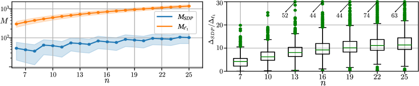
We evaluate the performance of reformulations with optimized , against the common choice for three examples of LCBO problem classes: Random sparse LCBOs, set partitioning problems (SPPs), and portfolio optimization (PO). Details on the model definitions and further results are presented in App. D.
For PO we use the well-known Markovitz model [32, 33, 34], i.e. the problem of selecting a set of assets maximizing returns while minimizing risk. The problem specification requires a vector of expected returns of a set of assets, their covariance matrix , a risk aversion , and a partition number defining the portfolio discretization. Denoting by the units of asset in the portfolio, the problem formulation reads
| (6) |
The constraint forces the budget to be totally invested. The QUBO reduction requires mapping each integer decision variable into binary variables. We generate problem instances from historic financial data on S&P 500 stocks.
We observe that the result of our algorithm is consistently one order of magnitude smaller than for random sparse LCBOs [Fig. 2 (a)] and SPPs [Fig. D.1 in App. D]. Concomitantly, the spectral gap is relatively increased by an order of magnitude [Fig. 2 (d)]. This corroborates our theoretic consideration relating optimized choices of to significantly improved spectral properties of the QUBO formulation. In the PO instances we additionally observe that the advantage in and further grows with the problem size [Fig. 2 (b) and (e)]. In contrast to random LCBOs and SPPs, PO has a single constraint independent of the problem size. While this allows for highly optimized choices of the penalty weight as exemplified by , the bound in Eq. (4) is oblivious to the intrinsic structure of PO. Using a greedy heuristic to determine (App. G), we further calculate for PO instances with up to binary variables and find that the improvements over persist [Fig. 2 (c)].
Quantum hardware deployment—.
Finally, after building our theoretical framework and numerical methods, we turn to the question of how relevant the Big- problem on actual noisy near-term hardware. To this end, we deployed toy instances of PO on the experimental -qubit trapped-ion quantum computer Aria-1 [35]. As an approximate solver, we executed a Trotterized adiabatic evolution to the Hamiltonians encoding QUBO reformulations (see App. F for implementation details). We executed a set of random six-qubit instances with a fixed budget of two-qubit gates for reformulations with and . The limit on the circuit size and a suitably chosen maximal evolution time determine the number of Trotterization steps. The parameter choice ensures approximate adiabaticity. We find that the probability of measuring the optimal solution is more than an order of magnitude higher with the reformulation than with [Fig. 2 (f)]. The probability of measuring the optimal solution determines the required number of repetitions and, thus, enters inversely into the time-to-solution. This behavior is consistently observed across all instances. Fig. 2 (g) shows the average approximation ratio—quantifying the quality of an approximate solution—over all measured outcomes that satisfy the budget constraint per instance. The formulations yield high ratios for most instances while the formulations perform comparable to classical uniform random sampling of solutions. Thus, already for small instances, we find that using an optimized is a prerequisite for deployment on noisy near-term hardware. Given the scaling observed in the numerical benchmarks, we expect that small values of are even more important for the performances that are not dominated by noise on intermediate sizes hardware.
Conclusions—.
On the conceptual side, we formalized the quantum big- problem, giving rigorous definitions, establishing its computational complexity, and giving bounds on the impact of on the spectral gap of the QUBO Hamiltonian. The latter relates the big- problem to performance guarantees of different solvers. From a practitioner’s viewpoint, our main contribution is a versatile QUBO reformulation algorithm with enhanced spectral properties, based on the SDP relaxation. Our mindset is that classical solvers should be leveraged to pre-condition problems so as to exploit quantum hardware to its maximal potential—near-term devices in particular. In numerical benchmarks, including Markovitz portfolio optimization (PO) instances from S&P 500 data, we consistently observe significant improvements in and the spectral gap using the proposed algorithm. In a six-qubit proof-of-principle experiment with trapped ions, we find that these improvements translate into a tangible advantage in the probability of measuring the correct solution.
Beyond near-term quantum devices, our analysis of the Big- problem also applies to future fault-tolerant quantum hardware, for instance in adiabatic schemes [5, 6] or quantum imaginary-time evolution simulations [8, 9, 10, 11, 12, 13, 14]. Besides, a particularly interesting question to explore is how beneficial our general big- recipe is for quantum-inspired, classical solvers [18, 19, 20]. Combining our approach with modern scalable randomized algorithms for SDPs [36] can potentially further reduce the complexity of calculating optimized values for . Finally, while our method was conceived for general instances, nuances of specific problems can enable heuristic tools for tighter lower bounds or feasible points, as already exemplified with the greedy heuristic for PO instances.
Acknowledgements—.
We thank Martin Kliesch and Marco Sciorilli for helpful comments.
References
- Abbas et al. [2023] A. Abbas et al., Quantum optimization: Potential, challenges, and the path forward, arXiv:2312.02279 [quant-ph] (2023).
- Montanaro [2015] A. Montanaro, Quantum algorithms: An overview, NPJ Quantum Information 2, 15023 (2015).
- Durr and Hoyer [1996] C. Durr and P. Hoyer, A quantum algorithm for finding the minimum, arXiv:quant-ph/9607014 (1996).
- Ambainis et al. [2019] A. Ambainis, K. Balodis, J. Iraids, M. Kokainis, K. Prūsis, and J. Vihrovs, Quantum speedups for exponential-time dynamic programming algorithms, in Proceedings of the Thirtieth Annual ACM-SIAM Symposium on Discrete Algorithms (SIAM, 2019) pp. 1783–1793.
- Farhi et al. [2000] E. Farhi, J. Goldstone, S. Gutmann, and M. Sipser, Quantum computation by adiabatic evolution, arXiv:quant-ph/0001106 (2000).
- Albash and Lidar [2018] T. Albash and D. A. Lidar, Adiabatic quantum computation, Rev. Mod. Phys. 90, 015002 (2018).
- Lang et al. [2022] J. Lang, S. Zielinski, and S. Feld, Strategic portfolio optimization using simulated, digital, and quantum annealing, Applied Sciences 12, 12288 (2022).
- McArdle et al. [2019] S. McArdle, T. Jones, S. Endo, Y. Li, S. Benjamin, and X. Yuan, Variational ansatz-based quantum simulation of imaginary time evolution, NPJ Quantum Information 5, 75 (2019).
- Motta et al. [2020] M. Motta, C. Sun, A. T. K. Tan, M. J. O’Rourke, E. Ye, A. J. Minnich, F. G. S. L. Brandão, and G. K.-L. Chan, Determining eigenstates and thermal states on a quantum computer using quantum imaginary time evolution, Nat. Phys. 16, 205 (2020).
- Nishi et al. [2021] H. Nishi, T. Kosugi, and Y. Matsushita, Implementation of quantum imaginary-time evolution method on nisq devices by introducing nonlocal approximation, NPJ Quantum Information 7, 85 (2021).
- Poulin and Wocjan [2009] D. Poulin and P. Wocjan, Sampling from the Thermal Quantum Gibbs State and Evaluating Partition Functions with a Quantum Computer, Physical Review Letters 103, 220502 (2009).
- Chowdhury and Somma [2017] A. N. Chowdhury and R. D. Somma, Quantum algorithms for gibbs sampling and hitting-time estimation, Quantum Inf. Comput. 17, 41 (2017).
- Wang et al. [2021] Y. Wang, G. Li, and X. Wang, Variational quantum gibbs state preparation with a truncated taylor series, arXiv:2005.08797 [quant-ph] (2021).
- Silva et al. [2023] T. d. L. Silva, M. M. Taddei, S. Carrazza, and L. Aolita, Fragmented imaginary-time evolution for early-stage quantum signal processors, Scientific Reports 13, 18258 (2023).
- Farhi et al. [2014] E. Farhi, J. Goldstone, and S. Gutmann, A quantum approximate optimization algorithm, arXiv:1411.4028 [quant-ph] (2014).
- Basso et al. [2022] J. Basso, E. Farhi, K. Marwaha, B. Villalonga, and L. Zhou, The Quantum Approximate Optimization Algorithm at High Depth for MaxCut on Large-Girth Regular Graphs and the Sherrington-Kirkpatrick Model, in 17th Conference on the Theory of Quantum Computation, Communication and Cryptography (TQC 2022), Vol. 232 (2022) pp. 7:1–7:21.
- He et al. [2023] Z. He et al., Alignment between initial state and mixer improves qaoa performance for constrained portfolio optimization, arXiv:2305.03857 [quant-ph] (2023).
- Goto et al. [2019] H. Goto, K. Tatsumura, and A. R. Dixon, Combinatorial optimization by simulating adiabatic bifurcations in nonlinear hamiltonian systems, Science Advances 5, eaav2372 (2019).
- Kanao and Goto [2022] T. Kanao and H. Goto, Simulated bifurcation assisted by thermal fluctuation, Nature Communications Physics 5, 153 (2022).
- Mohseni et al. [2022] N. Mohseni, P. L. McMahon, and T. Byrnes, Ising machines as hardware solvers of combinatorial optimization problems, Nature Review Physics 4, 363–379 (2022).
- Qiskit documentation [2022] Qiskit documentation, Converters for quadratic programs - linearequalitytopenalty (2022).
- Iosue [2020] J. T. Iosue, Welcome to qubovert’s documentation! (2020).
- Zaman et al. [2021] M. Zaman, K. Tanahashi, and S. Tanaka, Pyqubo: Python library for mapping combinatorial optimization problems to qubo form, IEEE Transactions on Computers 71, 838 (2021).
- Karimi and Ronagh [2019] S. Karimi and P. Ronagh, Practical integer-to-binary mapping for quantum annealers, Quantum Information Processing 18, 1 (2019).
- Harwood et al. [2021] S. Harwood, C. Gambella, D. Trenev, A. Simonetto, D. Bernal, and D. Greenberg, Formulating and solving routing problems on quantum computers, IEEE Transactions on Quantum Engineering 2, 1 (2021).
- Azad et al. [2023] U. Azad, B. K. Behera, E. A. Ahmed, P. K. Panigrahi, and A. Farouk, Solving vehicle routing problem using quantum approximate optimization algorithm, IEEE Transactions on Intelligent Transportation Systems 24, 7564 (2023).
- Leonidas et al. [2023] I. D. Leonidas, A. Dukakis, B. Tan, and D. G. Angelakis, Qubit efficient quantum algorithms for the vehicle routing problem on quantum computers of the nisq era, arXiv:2306.08507 (2023).
- Goemans and Williamson [1995] M. X. Goemans and D. P. Williamson, Improved approximation algorithms for maximum cut and satisfiability problems using semidefinite programming, Journal of the ACM (JACM) 42, 1115 (1995).
- Ebadi et al. [2022] S. Ebadi, A. Keesling, M. Cain, et al., Quantum optimization of maximum independent set using rydberg atom arrays, Science 376, 1209 (2022).
- Lucas [2014] A. Lucas, Ising formulations of many np problems, Frontiers in Physics 2, 5 (2014).
- Ayodele [2022] M. Ayodele, Penalty weights in qubo formulations: Permutation problems, in Evolutionary Computation in Combinatorial Optimization, Vol. 13222 (Springer International Publishing, 2022) pp. 159–174.
- Markowitz [1952] H. Markowitz, Portfolio selection, The Journal of Finance 7, 77 (1952).
- Grant et al. [2021] E. Grant, T. S. Humble, and B. Stump, Benchmarking quantum annealing controls with portfolio optimization, Phys. Rev. Applied 15, 014012 (2021).
- Rosenberg et al. [2016] G. Rosenberg, P. Haghnegahdar, P. Goddard, P. Carr, K. Wu, and M. L. de Prado, Solving the optimal trading trajectory problem using a quantum annealer, IEEE Journal of Selected Topics in Signal Processing 10, 1053 (2016).
- [35] Ionq trapped ion quantum computing.
- Yurtsever et al. [2021] A. Yurtsever, J. A. Tropp, O. Fercoq, M. Udell, and V. Cevher, Scalable semidefinite programming, SIAM Journal on Mathematics of Data Science 3, 171 (2021).
- McKay et al. [2017] D. C. McKay, C. J. Wood, S. Sheldon, J. M. Chow, and J. M. Gambetta, Efficient z gates for quantum computing, Physical Review A 96, 022330 (2017).
- Mølmer and Sørensen [1999] K. Mølmer and A. Sørensen, Multiparticle entanglement of hot trapped ions, Physical Review Letters 82, 1835 (1999).
- Solano et al. [1999] E. Solano, R. L. de Matos Filho, and N. Zagury, Deterministic bell states and measurement of the motional state of two trapped ions, Physical Review A 59, R2539 (1999).
- Trotter [1959] H. F. Trotter, On the product of semi-groups of operators, Proceedings of the American Mathematical Society 10, 545 (1959).
- Hatano and Suzuki [2005] N. Hatano and M. Suzuki, Finding exponential product formulas of higher orders, in Quantum annealing and other optimization methods, Vol. 679 (Springer Berlin Heidelberg, 2005) pp. 37–68.
- Efthymiou et al. [2021] S. Efthymiou, S. Ramos-Calderer, C. Bravo-Prieto, A. Pérez-Salinas, D. García-Martín, A. Garcia-Saez, J. I. Latorre, and S. Carrazza, Qibo: a framework for quantum simulation with hardware acceleration, Quantum Science and Technology 7, 015018 (2021).
- The Qibo team [2023] The Qibo team, qiboteam/qibo: Qibo 0.1.15 (2023).
- Ramos-Calderer [2023] S. Ramos-Calderer, quantum-bigm-trotterization (2023), https://github.com/igres26/quantum-bigM-trotterization.
Appendix A Gadgetization: from a general quadratically constrained quadratic optimization problem with integer variables to a linearly-constrained binary quadratic optimization problem
We present here the steps of a general procedure, often called gadgetization, consisting of elementary operations on the structure of a general combinatorial optimization problem, with the goal of reducing it to a simpler form, namely a quadratic binary problem with linear constraints. Let us consider a problem with quadratic objective function, integer decision variables and quadratic constraints which appear both with an equality and with an inequality condition. Notice that the mentioned formulation can also model polynomial functions, as one can map monomial terms with order greater than two to order two monomials, by adding additional variables to the model. This procedure is similar to what will be shown for the linearization of constraints. Such a problem will have the following form:
| (7) | ||||
| s.t. | (8) | |||
| (9) | ||||
| (10) | ||||
| (11) |
where and are, respectively, the number of equality and inequality constraints and the integer variables can have values in a finite set as they are upper bounded by some constants . Among the model parameters, , and are integer valued matrices and , and are -dimensional integer vectors. Notice that integer variables problems are often used to approximate real variables models. In such cases, by increasing the range that the integer variables span, it is possible to reach the desired correspondence between the discretized problem and the continuous one. As an example of this, the discretized Markowitz model in Portfolio Optimization has been analyzed in the present work.
In the rest of this section we present a four-step procedure that allows one to rewrite a problem in the form as a linearly-constrained binary quadratic optimization problem.
Step 1: rewriting the inequalities as equalities. In order to deal with equality constraints only, we first need to rewrite the inequalities as equalities, by using additional slack variables that compensate for the deviation between the two sides of the inequality. In this way, Eq. (9) will become
| (12) | |||
| (13) | |||
| (14) |
where . Observe that, although Eq. (13) may look like an inequality of the previous kind, it is actually much easier to deal with, since it does not relate variables among themselves. Rather, it only specifies the possible values every single integer variable can assume.
Step 2: binary expansion of the integer variables. Since the final formulation will have to contain binary decision variables only, a binary expansion of the integer variables is required, meaning that every integer variable will be replaced by a set of binary variables :
| (15) |
For the sake of clarity, in the following the superscript will be dropped from , as indicating to which integer variable every bit correspond to is not relevant in the present context. As for the expansion coefficients there exist many possible schemes, but here we pick a common one, called binary encoding, where .
Step 3: substitution of the quadratic terms in the quadratic equations. In order to deal with linear constraints only, we need to get rid of quadratic monomials of the form . It is possible to do so by defining a new binary variable
| (16) |
and substitute every appearance of such monomial with as a new decision variable. To enforce Eq. (16) it is enough to add to the objective function the term
| (17) |
Such a term adds a penalty factor only when Eq. (16) is not satisfied, therefore picking sufficiently large is equivalent to enforcing the substitution and therefore the linearization of the constraints overall.
Step 4: shifting the linear term in the objective function. In a model with only binary variables, it is possible to exploit the equivalence to rewrite the objective function as
| (18) |
The term indicates a square matrix with all the off-diagonal terms equal to zero, and the diagonal terms equal to . After the application of these four steps, we successfully recover the problem formulation in (1), the starting point in this present work.
Appendix B On the hardness of the quantum Big- problem
Here we formally establish that determining an optimal is in general as hard as finding the objective value of the original problem. We do this by proving a simple reduction from the decision-problem version of the latter to that of the former.
Finding the optimal objective value of a function under constraints is equivalent to an associated decision problem, decideF, which, given threshold and gap , decides if (‘smaller’) or if (‘greater’). Note that having access to an oracle for decideF allows one to efficiently find the optimal objective value via binary search. We want to relate the complexity of decideF to the following decision problem: Given an instance of (1), an , and a gap , decide if (2) with the given is an exact reformulation of (1) with gap at least (‘yes’) or (2) fails to be an exact reformulation (‘no’). We refer to this problem as decidePM. Note that decidePM is equivalent to the problem of finding the -optimal : Given an optimal value for , decidePM can be solved by comparing the under scrutiny to the optimal one. In turn, with an oracle for decidePM, the optimal can be found via binary search. Next, we prove the promised reduction.
Lemma 1.
The problem decideF reduces to decidePM.
Proof.
Consider an instance of decideF. W.l.o.g., we assume that the instance is unconstrained. For the constraint problem there exist a polynomial reduction to an unconstrained problem, e.g. using (2) with the value of defined in Eq. (4).
We will split decideF into decision problems where we decide the optimum for the subset with constant hamming weight . Deciding for all individually if (‘smaller’) or (‘greater’) allows us to solve decideF in the following way. If all constant-Hamming weight decisions return ‘greater’, we also conclude ‘greater’ for decideF. If at least one constant-Hamming weight decision returns ‘smaller’, we return ‘smaller’ for decideF. It is straight-forward to see that this strategy solves decideF correctly in both cases.
It remains to reduce the decision problem with constant Hamming weight to decidePM. For , i.e. , we can directly solve the decision problem by evaluation. If we find , we conclude ‘smaller’ for decideF. Thus, we can restrict our focus in the remainder to and assume that , where decideF is not yet decided. We choose , e.g. using defined in Eq. (4) for the quadratic form defining . Consider the following optimization problem:
| (19) |
The optimal point of (19) is the only feasible point with objective value . In other words, the constraint renders the optimization problem (19) trivial. Still of interest to us is the associated problem of deciding if certain values of yield unconstrained reformulations of (19). As formulated (19) is not an instance of (1), since the objective function is not quadratic. But the optimization problem (19) can be recast as the following binary quadratic problem:
| (20) |
Here the non-negative integer variables and can each be encoded with binary variables. The last summand dominates the objective function for all values of , and . Thus, at optimal and , it enforces the constraint . For the minimum of the objective function over and is attained when either or is equal to while the other variable vanishes. We conclude that for all the objective functions of (19) and (LABEL:eq:trivial_P_bqp) at optimal and coincide. Since (LABEL:eq:trivial_P_bqp) is an instance of (1), it defines instances of decidePM.
We now decide if (2) with is an exact reformulation with gap of (LABEL:eq:trivial_P_bqp). If the answer of decidePM is ‘yes’ (‘no’), we return ‘greater’ (‘smaller’). Our claim is that this strategy correctly solves the decision problem for the minimum of with constant Hamming-weight .
To see this, let us first consider the case ‘greater’, where . By our choice of , the QUBO reformulation of (LABEL:eq:trivial_P_bqp) with has an objective function that attains its minimum over the unfeasible points for . Thus, this minimum fulfills
| (21) |
Due to the trivializing constraint, is the optimal value of (LABEL:eq:trivial_P_bqp). Hence, (21) establishes the criterion Eq. (3) for an exact reformulation. As required in this case, decidePM, thus, returns ‘yes’ and we decide correctly.
Second, let us consider the case ‘smaller’, i.e. . By the same argument as before, we now find that the minimum of the objective function of the QUBO reformulation over the unfeasible points is smaller or equal than . Thus, decidePM returns ‘no’ in this case. Using decidePM, we therefore always arrive at the correct decision about the minimum of for constant Hamming-weight. ∎
Since decideF encompasses NP-complete problems like 3SAT, as a corollary of Lemma 1, we establish that finding the optimal value of is NP-hard.
Appendix C Bounds on the spectral gap of Big- QUBO reformulations
In this section, we provide the detailed argument for Observation 3 of the main text, and expand on some of its implications.
Let be a Hamiltonian encoding of (2). The normalized spectral gap of is defined as
| (22) |
where , and are the respective lowest, next-to-lowest and maximum energies of . We will study the behavior of compared to the corresponding quantity of the constraint optimization problem (1). To this end, let be an optimal point as before and let further be a next-to-optimal point of (1), i.e. the optimal point of (1) with the additional constraint . Denote by the constraint set and by its complement. We define the two upper bounds of the shifted objective function and . We refer to
| (23) |
as the spectral gap of (1).
(i) The Ising encoding ensures that for all , where denotes the basis vector that encodes the binary vector . For feasible, is in the kernel of . Thus, when is chosen such that (2) is an exact reformulation of (1), we have .
(ii) Analogously, is still in the spectrum of . Thus, . By Eq. (3) and assuming , we have . We conclude that (with the lower bound holding as long as does not exceed the upper bound). Note that the lower bound is saturated for the optimal . Also is still in the spectrum of . Hence, . All together, combined with (i) and its assumption, we arrive at the bound .
(iii) To infer the scaling of the spectral gap with , we note that , where we used the positivity of on the infeasible subspace and denote by the optimal , i.e. the minimal satisfying Eq. (3). Hence, . Thus, in particular .
Appendix D Benchmarked models
The present section illustrates the model definition and relevant details of the optimization problems tested, together with further results.
Random sparse LCBOs.
A general class of linearly-constrained binary quadratic optimization problems, whose formulation is (1), have been generated. We choose random instances for and with a bounded row-sparsity , i.e. , and similarly for . The non-vanishing entries of , and are uniformly drawn at random. We let the number of constraints grow linearly with the number of binary variables , specifically, .
Set partitioning problem (SPP).
Let be a subset of with an associated cost , for . A family of subsets is a partition of if and for all . The SPP consists of finding a partition of with minimal total cost:
| (24) |
The objective variables encode the subset family, with if is in the family and otherwise. The constraints force the family to be a partition of . We generate instances by randomly selecting constraint matrices with fixed density, i.e. number of non-zero entries over total number of entries. Fig. D.1 shows simulations results relative to this problem class.
Portfolio Optimization (PO).
The present paragraph illustrates how the data used in Portfolio Optimization instances were fetched from real data and adapted to Markowitz formulation (6). From stock market index S&P500, we downloaded the stock price history, referring to the 2 years period December 2020 until November 2022 with one-month interval, of 121 out of the 500 company stocks tracked by S&P500 (namely, the ones with no missing data in said intervals). Let us call such cost of an asset , with time index . The return at time step is defined as
| (25) |
from which the expected return vector and the covariance matrix can be easily computed:
We encode the real financial stock market data with decimal precision of .
Another parameter of the generated instances is the partition number [33], that describes the granularity of the portfolio discretization, since the budget is divided in equally large chunks. Each asset decision variable is an integer that can take values from up to , indicating how many of these partitions to allocate towards asset . This explains why the constraint enforces the budget to be totally invested. As a consequence, is also equal to the number of bits one needs to allocate for every integer and, by extension, asset. In the experiments we used a number of bits per asset .
Notice that is the expected return of a portfolio if represents the vector of the portions of the portfolio for each asset, i.e. and . In order to have integer decision variables, the number of chunks is used, and in the final formulation (6) of the Markowitz model the factors are absorbed in the objective function, defining and .
The last parameter that one needs to set to fully specify the instance is the risk aversion factor , weighting differently the return and the volatility in the objective function. In the experiments we used risk aversion factor .
Appendix E SDP Relaxation
The following optimization problem
| (26) | ||||
| (27) |
can be easily rewritten as
| (28) | ||||
| s.t. | (29) | |||
| (30) |
whereby we denote the dimensional column vector with as the first entry and as the remaining entries, while both and are matrices and denotes the inner product between matrices. In particular, the structure of the objective function is encapsulated in
| (31) |
The problem can be equivalently reformulated it in the context of convex optimization as
| (32) | ||||
| s.t. | (33) | |||
| (34) | ||||
| (35) | ||||
| (36) |
where we replaced condition (29) with (33), (34) and (35), while condition (30) becomes equivalent to (36), since .
Problem is thus equivalent to and its solution space can be viewed as a subset of the positive semi-definite matrices space, rather than the previous vector space. By removing constraints (34) and (35) we obtain formulation , also called SDP Relaxation, because it is a relaxation of formulation that consists of optimizing over the cone of semidefinite matrices intersected with linear constraints:
| (37) | ||||
| s.t. | (38) | |||
| (39) | ||||
| (40) |
In the formulation of an additional set of constraints (40) enforcing to have real entries in the interval is added to obtain stronger formulation. Clearly, solving provides a lower bound for , as .
Appendix F Experimental implementation
The adiabatic theorem [5, 6] states that a quantum system will remain in its instantaneous ground state through small perturbations to its Hamiltonian. Adiabatic quantum computation exploits this fact by preparing a system under the Hamiltonian
| (41) |
where is a Hamiltonian with an easy to prepare ground state, encodes the solution of a problem, and the schedule is evolved from to . If the evolution meets the conditions of the adiabatic theorem, the system will be at the ground state of at the end of the evolution, hence solving the problem.
A QUBO instance can be mapped into an Ising Hamiltonian by promoting each binary variable into quantum operators. Namely, by substituting for , where is the Pauli matrix acting on qubit . Namely, our problem Hamiltonian will be , by combining the objective function with the constraints . This way, we recover the diagonal matrix of the QUBO instance. The initial Hamiltonian is usually chosen as , as it has an easy to prepare ground state, the equal superposition of computational basis states. This is important, as one of the requirements for the evolution to work is a non-zero overlap between the initial and final ground states.
Deployment of algorithms on available quantum hardware requires precise fine-tuning as well as knowledge of the physical implementations of the device. In this work we target a gate-based ion trap quantum computer, as available through the IonQ cloud service [35]. The native interactions available in the device are the following: Single qubit gates are fixed and rotations along the plane, with precise control over the relative phase. Using this method, rotations around the axis are done virtually [37], and incur no noise. The IonQ aria-1 device allows for partially-entangling Mølmer-Sørenson [38, 39] gates, that is, a precisely tuned two qubit rotation along the plane with virtual control over the relative phases. Since the physics of the ion trap has access to a native interaction, we will perform a change of basis to the proposed Hamiltonian, so that the two-body terms in are combinations of , and comprises terms. Crucially, the ground state of the initial Hamiltonian is the starting state of the device, resulting in an even easier preparation for the purposes of our evolution.
The adiabatic evolution, ideally performed by slowly sweeping over the interaction parameters of the device, will need to be Trotterized [40, 41]. By selecting a total evolution time and a discretization step, the evolution can be approximately reproduced by single and two-qubit gates acting on the quantum device. Moreover, this method can be used to control the amount of quantum resources dedicated to solving the problem, which provides an equal starting point to test different QUBO encodings.
In order to conform with the device specifications, and compare different QUBO reformulations under the same conditions, we limit the number of two-qubit gates to . This corresponds to a final annealing time of with a Trotterization step of for the instances considered. The parameters used are far from an ideal adiabatic evolution, however, they should still result in an amplification of the ground state of the problem. As shown in Fig. 2 (f), this amplification is only significant using the reformulation, making it indispensable even for current noisy devices. This can also hint at advantages on more complex algorithms such as QAOA or VQE when encoding the problem using the proposed reformulation.
In approximate optimization, outputs that reach a high value for the objective function are desirable even if they do not maximize it. In order to quantify the quality of the solutions, we will use an approximation ratio. We define the approximation ratio used in this work as
| (42) |
if satisfies the constraints.
We build the Hamiltonian for the presented problem instances and Trotterize them using the quantum simulation library Qibo [42, 43]. Then, the resulting quantum circuits are parsed into native gate instructions for the IonQ aria-1 device. Code to reproduce this procedure is made available in the following Github repository [44].
Appendix G Greedy algorithm for Portfolio Optimization
Any strategy to get a feasible point using classical resources is a viable option to obtain via Eq. (5). For various classes of optimization problems, it is possible to apply a greedy heuristic algorithm to efficiently obtain a quasi-optimal point. To exemplify this, we describe a straight-forward greedy strategy for instances of Portfolio Optimization (6). Recall, that given assets and a partition number , the portfolio is discretized into equal fractions. The following algorithm aims at obtaining solutions by systematically allocating each portfolio portion to the asset that minimizes the objective function when evaluated on the existing segment of the portfolio.
Number of assets .
Partition number .