Cautious optimization via data informativity

Abstract

This paper deals with the problem of accurately determining guaranteed suboptimal values of an unknown cost function on the basis of noisy measurements. We consider a set-valued variant to regression where, instead of finding a best estimate of the cost function, we reason over all functions compatible with the measurements and apply robust methods explicitly in terms of the data. Our treatment provides data-based conditions under which closed-forms expressions of upper bounds of the unknown function can be obtained, and regularity properties like convexity and Lipschitzness can be established. These results allow us to provide tests for point- and set-wise verification of suboptimality, and tackle the cautious optimization of the unknown function in both one-shot and online scenarios. We showcase the versatility of the proposed methods in two control-relevant problems: data-driven contraction analysis of unknown nonlinear systems and suboptimal regulation with unknown dynamics and cost. Simulations illustrate our results.

1 Introduction

In many real-world applications involving optimization, the cost or reward function is not fully known and has to be ascertained from measurements. Such situations can arise due to a variety of factors, including system complexity, large-scale structure, or lack of access to the relevant information in unknown or adversarial scenarios. These considerations motivate the need for quantifiable performance guarantees that can be used for control and optimization in safety-critical applications. In this paper, we are therefore interested in cautious optimization of unknown functions, i.e., accurately determining guaranteed suboptimal values on the basis of noisy measurements. We consider both one-shot scenarios, where we are required to make decisions on the basis of a given set of data, and online scenarios, where the suboptimization of the unknown function can be repeatedly refined based on the collection of additional measurements. Our approach, based on data informativity, allows us to derive results which are robust against worst-case situations.

Literature review: Data-based optimization is a widely applicable and thoroughly investigated area. Giving a full overview of all methods and results is not possible, and thus we focus here on those most relevant to our treatment. The problems considered here are robust optimization programs, see e.g. [2, 3] and references therein. Solution approaches to data-based optimization problems usually start by using the data to obtain an estimate of the unknown function which in some sense ‘best’ explains the measurements. This requires the definition of the class of admissible functions. Popular nonparametric techniques are based on Gaussian processes, as in [4], the approximation properties of neural networks [8, 9], and of particular relevance to our analysis here is the work on set-membership identification [5, 6, 7]. These works consider similar set-valued uncertainties, on the basis of Lipschitz interpolation.

In contrast, we make use of basis functions, where the unknown function is parameterized by a linear combination of the basis. Choices that balance expressiveness and the number of parameters are linear, polynomials, Gaussian, and sigmoidal functions. Depending on the problem, one may also choose a basis by taking into account physical considerations or emplying spectral methods [10, 11, 12]. Once a basis is chosen, the data is used to perform regression [13, 14] on the parameters. What remains to be defined is then the metric chosen to decide the best estimate. Common methods are least squares (minimal Frobenius norm), ridge regression (minimal $L_{2}$ norm), sparse or Lasso regression (minimal $L_{1}$ norm). The nonlinear system-identification literature has also brought forward methods which determine models that are sparse [15], of low rank (via dynamic mode decomposition) [16, 17, 18], or both [19]. Regardless of how one obtains an estimate, the second step in data-based optimization is to employ either a certainty-equivalent or robust method to find optimal values.

The alternative approach we use here is in line with the literature of data-driven control methods on the basis of Willems’ fundamental lemma [20]. More specifically, we consider the concept of data informativity [21]. Simply put, these methods take the viewpoint that guaranteed conclusions can be drawn from data only if all systems compatible with the measurements have this property. Of specific interest to this paper are works that deal with nonlinear systems and a number of recent works have worked with systems given in terms of bilinear [22] or polynomial basis functions [23, 24], albeit in discrete time. Simultaneously, there haven been efforts in generalizing Willems’ lemma to continuous time [25, 26] and linking the results in discrete and continuous time by investigating sampling [27].

Our applications here concern data-based contraction analysis of nonlinear systems [28, 29] and the regulation of an unknown system to the suboptimal point of an unknown cost function. Data-based regulation with a known cost function has been investigated in a number of forms, including linear quadratic regulation, see [30] and references therein, and more general cost functions via optimization-based controllers [31, 32]. In [33], such controllers have been employed to optimize unknown cost functions. Finally, the online optimization scenario considered here is inspired by methods such as extremum-seeking control [34, 35, 36]. However, our implementation and performance guarantees are of a markedly different nature.

Statement of contributions: We tackle the data-based optimization of an unknown vector-valued function with the goal of obtaining quantifiable performance guarantees. Starting from the assumption that the unknown function is parameterized in terms of a finite number of basis functions, we consider set-valued regression, i.e., we reason with the set of all parameters compatible with the measurements for which the noise satisfies a bound given in terms of a quadratic matrix inequality. We take a worst-case approach regarding noise realizations, leading us to provide solutions to the following cautious optimization problems:

1. We provide conditions in terms of the measurements, basis functions, and noise model which guarantee that either the $2-$norm or a linear functional of the unknown function is upper bounded by a given $\delta\in\mathbb{R}$ for a given $z\in\mathbb{R}^{n}$. Moreover, these results make it possible for us to find the smallest worst-case bounds;

2. We also provide data-based conditions for convexity of either the true function or its worst-case norm bounds. These allow us to introduce a gradient-based method for finding the minimizer of the upper bound;

3. We also identify data-based conditions for Lipschitzness which, using interpolation, allows us to derive upper bounds guaranteed to hold over compact sets.

We illustrate the versatility of the results in two application scenarios: contraction analysis of nonlinear systems (for which we provide data-based tests to determine one-sided Lipschitz constants and use them to guarantee contractivity) and suboptimal regulation of unknown plants with unknown cost functions (for which we employ convexity and Lipschitzness to find a fixed input such that the value of the cost function at the corresponding fixed point can be explicitly bounded above). Our final contribution is to online data-based optimization. We describe a framework for incorporating new measurements of the unknown function which includes online local descent, a method that iteratively collects measurements locally and then minimizes an upper bound of the form described above. We prove that under mild assumptions on the collection of data, the set of parameters consistent with all collected measurements shrinks. This allows us to conclude that the upper bounds found with online local descent converge to the true optimizer of the unknown function.

Preliminary results of this paper were presented in the conference article [1], whose focus was restricted to scalar functions and provided upper bounds and analyzed convexity on the basis of data. The conference paper also presented a simplified version of online local descent for the scalar case. All of these are special cases of the present work. Note that the generalization here from scalar to vector-valued functions is instrumental in expanding the range of possibilities for application in analysis and control of the proposed data-based optimization framework.

Notation: Throughout the paper, we use the following notation. We denote by $\mathbb{N}$ and $\mathbb{R}$ the sets of nonnegative integer and real numbers, respectively. We let $\mathbb{R}^{n\times m}$ denote the space of $n\times m$ real matrices and $\mathbb{S}^{n}$ the space of symmetric $n\times n$ matrices. For a vector $x\in\mathbb{R}^{n}$ we denote the standard $p-$norm by $\|x\|_{p}$. Given $R\in\mathbb{R}^{n\times n}$, we define the weighted $p-$norm by $\|x\|_{p,R}:=\|Rx\|_{p}$. The $i^{\textrm{th}}$ standard basis vector is denoted $e_{i}$. The induced matrix norm w.r.t. to the $p-$norm is denoted $\|A\|_{p}$ for $A\in\mathbb{R}^{n\times m}$. For vectors $v\in\mathbb{R}^{n}$, we write $v\geqslant 0$ (resp. $v>0$) for elementwise nonnegativity (resp. positivity). The sets of such vectors are denoted $\mathbb{R}^{n}_{\geqslant 0}:=\{v\in\mathbb{R}^{n}|v\geqslant 0\}$ and $\mathbb{R}^{n}_{>0}:=\{v\in\mathbb{R}^{n}|v>0\}$. For $P\in\mathbb{S}^{n}$, $P\geqslant 0$ (resp. $P>0$) denotes that $P$ is symmetric positive semi-definite (resp. definite). For a square matrix $M$, we denote $\lambda_{\textup{min}}(M)$ and $\lambda_{\textup{max}}(M)$ for the smallest and largest eigenvalue of $M$. We denote the smallest singular value of $M\in\mathbb{R}^{n\times m}$ by $\sigma_{-}(M)$ and its Moore-Penrose pseudoinverse by $M^{\dagger}$. The convex hull and interior of $\mathcal{S}\subseteq\mathbb{R}^{n}$ are denoted by $\operatorname{conv}(\mathcal{S})$ and $\operatorname{int}(\mathcal{S})$, resp. Given a symmetric matrix $M\in\mathbb{S}^{u+v}$, when $u$ and $v$ are clear from context, we partition it as:

$$M=\bigg{[}\begin{matrix}M_{11}&M_{12}\\ M_{21}&M_{22}\end{matrix}\bigg{]},$$

where $M_{11}\in\mathbb{S}^{u}$ and $M_{22}\in\mathbb{S}^{v}$. We denote the Schur complement of $M$ with respect to $M_{22}$ by $M|M_{22}:=M_{11}-M_{12}M_{22}^{\dagger}M_{21}$. Lastly, a partitioned matrix gives rise to a a quadratic matrix inequality (QMI), whose set of solutions is denoted by

$$\mathcal{Z}(M):=\bigg{\{}Z\in\mathbb{R}^{v\times u}\mid\begin{bmatrix}I_{u}\\ Z\end{bmatrix}^{\top}\!\!M\begin{bmatrix}I_{u}\\ Z\end{bmatrix}\geqslant 0\bigg{\}}.$$

2 Problem formulation

Consider a collection of known basis functions (or features), denoted $\phi_{i}:\mathbb{R}^{n}\rightarrow\mathbb{R}$ for $i=1,\ldots,k$. For ease of notation, we collect the basis functions into a vector-function as

$$\vspace{-0.3em}b:\mathbb{R}^{n}\rightarrow\mathbb{R}^{k},\quad b(z):=\begin{bmatrix}\phi_{1}(z)^{\top}&\cdots&\phi_{k}(z)^{\top}\end{bmatrix}^{\top}.$$ (1)

On the basis of these basis functions, we define linear combinations as parameterized by $\theta\in\mathbb{R}^{k\times m}$:

$$\vspace{-0.3em}\phi^{\theta}:\mathbb{R}^{n}\rightarrow\mathbb{R}^{m},\quad\phi^{\theta}(z)=\theta^{\top}b(z).$$

Our starting point is an unknown function $\hat{\phi}:\mathbb{R}^{n}\rightarrow\mathbb{R}^{m}$ that can be expressed in this form: i.e., there exists $\hat{\theta}\in\mathbb{R}^{k\times m}$ such that $\hat{\phi}(z)=\hat{\theta}^{\top}b(z)$.

Our goal is to investigate properties and optimize the unknown function $\hat{\phi}$ on the basis of measurements at points $\{z_{i}\}_{i=1}^{T}$. We assume the measurements are noisy, that is, we collect $y_{i}=\hat{\phi}(z_{i})+w_{i}$, where $w_{i}$ denotes an unknown disturbance vector for each $i$. To express this in compact form, define the matrices $Y,W\in\mathbb{R}^{m\times T}$ and $\Phi\in\mathbb{R}^{k\times T}$ by

$$\begin{split}&Y:=\begin{bmatrix}y_{1}&\cdots&y_{T}\end{bmatrix},\;\quad W:=\begin{bmatrix}w_{1}&\cdots&w_{T}\end{bmatrix},\\ &\Phi:=\scriptsize\begin{bmatrix}b(z_{1})&\cdots&b(z_{T})\end{bmatrix}=\begin{bmatrix}\phi_{1}(z_{1})&\dots&\phi_{1}(z_{T})\\ \vdots&&\vdots\\ \phi_{k}(z_{1})&\dots&\phi_{k}(z_{T})\end{bmatrix}.\end{split}$$ (2)

Then, for the true value of $\hat{\theta}$, we have $Y=\hat{\theta}^{\top}\Phi+W$. In this equation, the matrices $Y$ and $\Phi$ are known, and $\hat{\theta}$ and $W$ are unknown.

A common line of reasoning (see e.g., [13]) to approximate the unknown function $\hat{\phi}$ is the following. Assuming that small noise samples are more probable than large noise samples, we attempt to find a solution $\theta$ to $Y=\theta^{\top}\Phi+W$ for which the Frobenius norm of $W$, denoted $\|W\|_{F}$, is as small as possible. This can be formulated as

$$\vspace{-0.3em}\operatorname*{arg\,min}_{\theta}\|Y-\theta^{\top}\Phi\|_{F}=(Y\Phi^{\dagger})^{\top}.$$

Here instead we consider bounded noise and reason with the set of functions consistent with the measurements. Formally, we assume that the noise conforms to a model defined by a QMI given in terms of a partitioned matrix. The following assumption describes the noise model.

Assumption 1 (Noise model).

We assume that the noise samples satisfy $W^{\top}\in\mathcal{Z}(\Pi)$, where $\Pi\in\mathbb{S}^{m+T}$ is such that $\Pi_{22}<0$ and $\Pi|\Pi_{22}\geqslant 0$.

According to [37, Thm. 3.2], under Assumption 1, the set $\mathcal{Z}(\Pi)$ is nonempty, convex, and bounded. A common example of such noise models is the case where $WW^{\top}=\sum_{i=1}^{T}w_{i}w_{i}^{\top}\leqslant Q$ for some $Q\geqslant 0$. In addition, in the setting of Gaussian noise, these noise models can be employed as confidence intervals corresponding to a given probability.

Under Assumption 1, one can describe the set of parameters consistent with the measurements as

$$\vspace{-0.3em}\Theta=\{\theta\in\mathbb{R}^{k\times m}\mid Y=\theta^{\top}\Phi+W,W^{\top}\in\mathcal{Z}(\Pi)\}.$$ (3)

Note that we can write

$$\vspace{-0.3em}Y=\theta^{\top}\Phi+W\iff\begin{bmatrix}I_{m}&W\end{bmatrix}=\begin{bmatrix}I_{m}&\theta^{\top}\end{bmatrix}\begin{bmatrix}I_{m}&Y\\ 0&-\Phi\end{bmatrix}.$$

Thus, if we define

$$\vspace{-0.3em}N:=\begin{bmatrix}I_{m}&Y\\ 0&-\Phi\end{bmatrix}\Pi\begin{bmatrix}I_{m}&Y\\ 0&-\Phi\end{bmatrix}^{\top},$$ (4)

it follows immediately that $\Theta=\mathcal{Z}(N)$. We refer to the procedure of obtaining the set of parameters $\Theta$ from the measurements as set-valued regression.

Remark 2.1.

(Sufficiently exciting measurements) Note that the set $\Theta$ is compact if and only if $N_{22}<0$. Since $N_{22}=\Phi\Pi_{22}\Phi^{\top}$ and $\Pi_{22}<0$, this holds if and only if $\Phi$ has full row rank. In turn, this requires that the basis functions are not identical and that the set of points $\{z_{i}\}_{i=1}^{T}$ where measurements are taken is ‘rich’ enough or sufficiently ‘exciting’, cf. [20]. $\bullet$

Remark 2.2.

(Least-squares estimate) One can check that, under Assumption 1, $\theta^{\operatorname{lse}}:=-N_{22}^{\dagger}N_{21}\in\Theta$. This means that the function $(\theta^{\operatorname{lse}})^{\top}b(z)$ is consistent with the measurements. In fact,

$$\scriptsize N|N_{22}=\begin{bmatrix}I_{m}\\ -N_{22}^{\dagger}N_{21}\end{bmatrix}^{\top}N\begin{bmatrix}I_{m}\\ -N_{22}^{\dagger}N_{21}\end{bmatrix}\geqslant\begin{bmatrix}I_{m}\\ \theta\end{bmatrix}^{\top}N\begin{bmatrix}I_{m}\\ \theta\end{bmatrix},$$

for any $\theta^{\top}\in\mathcal{Z}(N)$. Therefore, $\theta^{\operatorname{lse}}$ is the value that maximizes the value of the quadratic inequality. This leads us to refer to the function $\phi^{\operatorname{lse}}(z;\Theta):=(\theta^{\operatorname{lse}})^{\top}b(z)=-N_{12}N_{22}^{\dagger}b(z)$ as the least-squares estimate of $\hat{\phi}(z)$. $\bullet$

In regards to the optimization of $\hat{\phi}$, note that changes in the parameter $\theta$ might lead to changes in the quantitative behavior and in particular the location of optimal values of the functions $\phi^{\theta}$. This means that a small error in estimating the true parameter corresponding to the unknown function $\hat{\phi}$ might lead to significant error. This motivates us to focus on suboptimization problems instead. To be precise, we investigate whether, for a given $\delta\in\mathbb{R}$ and $c\in\mathbb{R}^{m}$, we can ensure that

$$\|\hat{\phi}(z)\|_{2}\leqslant\delta\quad\textrm{ or }\quad c^{\top}\hat{\phi}(z)\leqslant\delta.$$ (5)

Thus the following problem statement.

Problem 1 (Cautious optimization).

Consider an unknown function $\hat{\phi}:\mathbb{R}^{n}\rightarrow\mathbb{R}^{m}$, a noise model $\Pi$ such that Assumption 1 holds, data $(Y,\Phi)$ of the true function, and the set $\Theta$ as in (3). Then

1. (Verification of suboptimality) given $z\in\mathbb{R}^{n}$, determine the minimal value of $\delta\in\mathbb{R}$ for which we can guarantee that either inequality in (5) holds;

2. (One-shot cautious suboptimization) given a set $\mathcal{S}\subseteq\mathbb{R}^{n}$, find $z\in\mathcal{S}$ for which Problem 1(i) yields the minimal value of $\delta$;

3. (Set-wise verification of suboptimality) given a set $\mathcal{S}\subseteq\mathbb{R}^{n}$, find the minimal $\delta\in\mathbb{R}$ for which either inequality in (5) holds for all $z\in\mathcal{S}$.

We note that being able to resolve any of these problems can be viewed as a property of the measurements, which is the viewpoint taken in the data informativity framework, e.g., [21, 37]: given $\delta\in\mathbb{R}$ and $\mathcal{S}\subseteq\mathbb{R}^{n}$, one could say that the data $(Y,\Phi)$ is informative for $\delta$-suboptimization on $\mathcal{S}$ if there exists $z\in\mathcal{S}$ such that $\|\hat{\phi}(z)\|_{2}\leqslant\delta$.

We rely on the data informativity interpretation throughout our technical discussion in Section 3 to solve Problem 1. Then, in Section 4, we illustrate how to apply our results to solve various problems in data-driven analysis and control. First, we consider data-based contraction analysis for a class of nonlinear systems parameterized in terms of given basis functions. This essentially requires us to characterize one-sided Lipschitz constants for the unknown dynamics in terms of measured data. In terms of data-driven control, we consider the problem of data-based suboptimal regulation of unknown linear systems. Finally, in Section 5 we analyze various formulations of online suboptimization, where we iteratively optimize and collect new measurements to find the optimizer.

3 Cautious optimization

This section describes our solutions to Problem 1. Recall that, based on the data, we cannot distinguish $\hat{\phi}$ from any of the functions $\phi^{\theta}$ as long as $\theta\in\Theta$. This means that we can only guarantee that $\|\hat{\phi}(z)\|_{2}\leqslant\delta$ holds if $\sup_{\theta\in\Theta}\|\phi^{\theta}(z)\|_{2}\leqslant\delta$. Similarly, given a vector $c\in\mathbb{R}^{m}$, we can only conclude that $c^{\top}\hat{\phi}(z)\leqslant\delta$ if $\sup_{\theta\in\Theta}c^{\top}\phi^{\theta}(z)\leqslant\delta$. This motivates the following definitions:

$$g(z;\Theta):=\sup_{\theta\in\Theta}\|\phi^{\theta}(z)\|_{2},\quad g_{c}(z;\Theta):=\sup_{\theta\in\Theta}c^{\top}\phi^{\theta}(z).$$ (6)

These functions correspond to the elementwise worst-case realization of the unknown parameter $\hat{\theta}$. Therefore, we refer to $g(z;\Theta)$ as the worst-case norm bound and $g_{c}(z;\Theta)$ as the worst-case linear bound.

To draw conclusions regarding the true function $\hat{\phi}$, we investigate the functions $g(z;\Theta)$ and $g_{c}(z;\Theta)$. In fact, problems (i)-(iii) in Problem 1 can be recast as follows. Resolving Problem 1(i) (in Section 3.1) boils down to finding function values of $g(z;\Theta)$ or $g_{c}(z;\Theta)$. Resolving Problem 1(ii) (in Section 3.3) is equivalent to finding

$$\vspace{-0.3em}\min_{z\in\mathcal{S}}g(z;\Theta)\quad\textrm{ or }\quad\min_{z\in\mathcal{S}}g_{c}(z;\Theta).$$ (7)

Finally, resolving Problem 1(iii) (in Section 3.4) amounts to finding the minimal $\delta$ for which

$$\vspace{-0.3em}\max_{z\in\mathcal{S}}g(z;\Theta)\leqslant\delta\quad\textrm{ or }\quad\max_{z\in\mathcal{S}}g_{c}(z;\Theta)\leqslant\delta.$$ (8)

3.1 Pointwise verification of suboptimality

In order to resolve Problem 1(i), we are interested in obtaining values of the functions in (6). As a first observation, note that if the set $\Theta$ is compact (cf. Remark 2.1), then the supremum is attained, and we can replace it with a maximum. In this case, the worst-case norm bound and worst-case linear bound are finite-valued functions.

We rely on the following characterization to obtain function values of $g(z;\Theta)$.

Lemma 3.1.

(Data-based conditions for bounds on the norm) Given data $(Y,\Phi)$, let $\Theta=\mathcal{Z}(N)$, with $N$ as in (4). Suppose that $N$ has at least one positive eigenvalue. Let $\delta\geqslant 0$ and $z\in\mathbb{R}^{n}$. Then,

$$\vspace{-0.3em}\|\phi^{\theta}(z)\|_{2}\leqslant\delta\quad\textrm{ for all }\quad\theta\in\Theta$$ (9)

if and only if there exists $\alpha\geqslant 0$ such that

$$\vspace{-0.3em}\scriptsize\left[\vbox{\hbox{\kern-1.1563pt\raise 0.0pt\hbox{\kern 39.2118pt}\kern 0.0pt\vbox{}\kern-1.1563pt}}\right]\normalsize-\alpha\left[\vbox{\hbox{\kern-1.1563pt\raise 0.0pt\hbox{\kern 14.12498pt}\kern 0.0pt\vbox{}\kern-1.1563pt}}\right]\geqslant 0.$$ (10)

Note that $\|\phi^{\theta}(z)\|^{2}_{2}=b(z)^{\top}\theta\theta^{\top}b(z)$. This allows us to write (9) equivalently as

$$b(z)^{\top}\theta\theta^{\top}b(z)\leqslant\delta^{2}\iff\theta^{\top}b(z)b(z)^{\top}\theta\leqslant\delta^{2}I_{m},$$

which can also be expressed as

$$\vspace{-0.3em}\scriptsize\begin{bmatrix}I_{m}\\ \theta\end{bmatrix}^{\top}\begin{bmatrix}\delta^{2}I_{m}&0\\ 0&-b(z)b(z)^{\top}\end{bmatrix}\begin{bmatrix}I_{m}\\ \theta\end{bmatrix}\geqslant 0.$$ (11)

Thus (9) holds if and only if (11) holds for all $\theta\in\Theta$. Given that $\Theta=\mathcal{Z}(N)$, where $N$ has at least one positive eigenvalue, the statement follows from applying [37, Thm 4.7] to (11) and using a Schur complement. $\blacksquare$

The necessary and sufficient conditions of Lemma 3.1 allow us to provide an alternative expression for $g(z;\Theta)$ that allows us to compute its value efficiently.

Corollary 3.2.

(Values of the worst-case norm bound) Given data $(Y,\Phi)$, let $\Theta=\mathcal{Z}(N)$, with $N$ as in (4). Suppose that $N$ has at least one positive eigenvalue. For $z\in\mathbb{R}^{n}$, we have

$$g(z;\Theta)=\min\{\delta\geqslant 0\mid\exists\alpha\geqslant 0\textrm{ s.t. }\eqref{eq:LMI cond norm}\textrm{ holds}\}.$$ (12)

Note that technically, the statement (10) is not an LMI. However, since (10) is linear in $\delta^{2}$, function values of $g(z;\Theta)$ can be found efficiently via Corollary 3.2. Similar situations pass without mention in the remainder of this paper.

Remark 3.3.

(Weakening assumptions on data lead to conservative upper bound)If $N$ does not have positive eigenvalues, i.e., $N\leqslant 0$, then the ‘if’-side of Lemma 3.1 remains true. Therefore, we can conclude that (12) in Corollary 3.2 holds with ‘$\leqslant$’ replacing ‘$=$’. This means that we obtain an upper bound for $g(z;\Theta)$, leading to a conservative upper bound of $\hat{\phi}(z)$. $\bullet$

Moreover, we can use Corollary 3.2 to find bounds independent of the choice of $z$.

Remark 3.4.

(Relaxations of the conditions for bounds on the norm) If $M$ is such that $b(z)b(z)^{\top}\leqslant M$, then

$$\scriptsize\begin{bmatrix}\delta^{2}I_{m}&0\\ 0&-b(z)b(z)^{\top}\end{bmatrix}\geqslant\begin{bmatrix}\delta^{2}I_{m}&0\\ 0&-M\end{bmatrix}.$$

This implies that

$$\vspace{-0.3em}\scriptsize\begin{bmatrix}\delta^{2}I_{m}&0\\ 0&-M\end{bmatrix}\normalsize-\alpha N\geqslant 0$$ (13)

implies (10). In turn, this means that for any $M$ such that $b(z)b(z)^{\top}\leqslant M$ for all $z$, we have

$$g(z;\Theta)\leqslant\min\{\delta\geqslant 0\mid\exists\alpha\geqslant 0\textrm{ s.t. }\eqref{eq:cond in norm of b}\textrm{ holds}\},$$

which yields a bound independent from $z$. $\bullet$

We rely on the following characterization to obtain function values of $g_{c}(z;\Theta)$.

Lemma 3.5.

(Data-based conditions for scalar upper bounds) Given data $(Y,\Phi)$, let $\Theta=\mathcal{Z}(N)$, with $N$ as in (4). Let $\delta\in\mathbb{R}$, $z\in\mathbb{R}^{n}$, and $c\in\mathbb{R}^{m}$. Suppose $c^{\top}(N|N_{22})c>0$ and let

$$\vspace{-0.3em}N_{c}:=\begin{bmatrix}c^{\top}N_{11}c&c^{\top}N_{12}\\ N_{21}c&N_{22}\end{bmatrix}.$$ (14)

Then it holds that

$$c^{\top}\phi^{\theta}(z)\leqslant\delta\quad\textrm{ for all }\quad\theta\in\Theta$$ (15)

if and only if there exists $\alpha\geqslant 0$ such that

$$\begin{bmatrix}2\delta&-b(z)^{\top}\\ -b(z)&0\end{bmatrix}-\alpha N_{c}\geqslant 0.$$ (16)

We can rewrite $c^{\top}\phi^{\theta}(z)$ as $c^{\top}\theta^{\top}b(z)+b(z)^{\top}\theta c\leqslant 2\delta$. Thus, (15) holds if and only if

$$\gamma^{\top}b(z)+b(z)^{\top}\gamma\leqslant 2\delta\quad\textrm{ for all }\quad\gamma\in\mathcal{Z}(N)c,$$

where $\mathcal{Z}(N)c:=\{Zc\mid Z\in\mathcal{Z}(N)\}$. Since $c\neq 0$, by [37, Thm. 3.4], we have $\mathcal{Z}(N)c=\mathcal{Z}(N_{c})$. Therefore, (15) is equivalent to:

$$\vspace{-0.3em}\scriptsize{\begin{bmatrix}1\\ \gamma\end{bmatrix}^{\top}\begin{bmatrix}2\delta&-b(z)^{\top}\\ -b(z)&0\end{bmatrix}\begin{bmatrix}1\\ \gamma\end{bmatrix}}\normalsize\geqslant 0,\textrm{ for all }\gamma\in\mathcal{Z}(N_{c}).$$ (17)

Given that $N_{22}\leqslant 0$, we have that $c^{\top}(N|N_{22})c>0$ if and only if $N_{c}$ has a positive eigenvalue. Then, the statement follows from applying [37, Thm 4.7] to (17). $\blacksquare$ We leverage the characterization in Lemma 3.5 to provide a closed-form expression of $g_{c}(z;\Theta)$ in terms of the data.

Theorem 3.6.

(Explicit bounds in the scalar case) Given data $(Y,\Phi)$, let $\Theta=\mathcal{Z}(N)$, with $N$ as in (4). Let $z\in\mathbb{R}^{n}$ and $c\in\mathbb{R}^{m}$. If $b(z)\in\operatorname{im}\Phi$ or $c=0$, then

$$\begin{split}\vspace{-0.3em}g_{c}(z;\Theta)=&-c^{\top}N_{12}N_{22}^{\dagger}b(z)\\ &\quad+\sqrt{c^{\top}(N|N_{22})cb(z)^{\top}(-N_{22}^{\dagger})b(z)},\end{split}$$

and, if $c\neq 0$ and $b(z)\not\in\operatorname{im}\Phi$, then $g_{c}(z;\Theta)=\infty$.

Note that, if either $c=0$ or $b(z)=0$, then we have $g_{c}(z;\Theta)=0$, thus the result follows. Assume then that $c\neq 0$, $b(z)\neq 0$, and $b(z)\in\operatorname{im}\Phi$. If $c^{\top}(N|N_{22})c=0$, then $N_{c}\leqslant 0$. As such, $\gamma\in\mathcal{Z}(N_{c})$ if and only if

$$\vspace{-0.3em}N_{c}\begin{bmatrix}1\\ \gamma\end{bmatrix}=0\iff\gamma\in-N_{22}^{\dagger}N_{21}c+\ker N_{22}.$$

Using (17), we see that $c^{\top}\phi^{\theta}\leqslant\delta$ for all $\theta\in\Theta$ if and only if $\gamma^{\top}b(z)\leqslant\delta$ for all $\gamma\in\mathcal{Z}(N_{c})$. Combining the previous, we see that this holds if and only if $\delta\geqslant-c^{\top}N_{12}N_{22}^{\dagger}b(z)$ (where we have used that $b(z)\in\operatorname{im}\Phi$). Minimizing $\delta$ reveals that the statement holds for this case.

Consider the case when $c^{\top}(N|N_{22})c>0$. By Lemma 3.5, (15) holds if and only if (16) holds for some $\alpha\geq 0$. Since $b(z)\neq 0$, it must be that $\alpha>0$. Using the Schur complement on (16), we obtain

$$\vspace{-0.3em}0 \leqslant\!2\delta\!-\!\alpha c^{\!\top}N_{11}c+\alpha^{\!-1}(b(z)^{\!\top}+\alpha c^{\!\top}N_{12})N_{22}^{\dagger}(b(z)\!\!+\alpha N_{21}c)$$

$$=2\delta+c^{\top}N_{12}N_{22}^{\dagger}b(z)+b(z)^{\top}N_{22}^{\dagger}N_{21}c$$

$$\quad-\alpha c^{\top}(N|N_{22})c+\alpha^{-1}b(z)^{\top}N_{22}^{\dagger}b(z).$$

Clearly, there exists $\alpha$ for which this holds if and only if it holds for the value of $\alpha$ that maximizes the expression on the right. Note that $\ker N_{22}=\ker\Phi^{\top}$. Thus, since $b(z)\in\operatorname{im}\Phi$ and $b(z)\neq 0$, we see that $b(z)^{\top}N_{22}^{\dagger}b(z)<0$. The expression is then maximized over $\alpha\geqslant 0$ with

$$\vspace{-0.3em}\alpha=\sqrt{\frac{-b(z)^{\top}N_{22}^{\dagger}b(z)}{c^{\top}(N|N_{22})c}}.$$

This yields that (16) holds if and only if

$$2\delta+c^{\top}N_{12}N_{22}^{\dagger}b(z)+b(z)^{\top}N_{22}^{\dagger}N_{21}c$$

$$-2\sqrt{c^{\top}(N|N_{22})cb(z)^{\top}(-N_{22}^{\dagger})b(z)}\geqslant 0.$$

To obtain $g_{c}(z;\Theta)$, we minimize this over $\delta$, which yields the expression in the statement.

Finally, consider the case when $c\neq 0$ and $b(z)\not\in\operatorname{im}\Phi$. It is straightforward to check that if $\theta\in\Theta$, then $\theta+vw^{\top}\in\Theta$, for all $w\in\mathbb{R}^{m}$ and $v\in\ker\Phi^{\top}\subseteq\mathbb{R}^{k}$. Since $b(z)\not\in\operatorname{im}\Phi$ and $\operatorname{im}\Phi$ is orthogonal to $\ker\Phi^{\top}$, we can take $v$ such that $v^{\top}b(z)>0$. Now, for arbitrary $\beta\in\mathbb{R}$, take $w=\beta c$. Then,

$$\sup_{\theta\in\Theta}\phi^{\theta}(z)\geqslant c^{\top}(\theta+vw^{\top})^{\top}b(z)=c^{\top}\theta^{\top}b(z)+\beta c^{\top}cv^{\top}b(z).$$

Since $c^{\top}c>0$ and $v^{\top}b(z)>0$, and this is valid for any $\beta\in\mathbb{R}$, the last part of the statement follows. $\blacksquare$

Remark 3.7 (The special case of $N_{22}<0$).

Note that when $\Theta$ is compact (or equivalently, $\Phi$ has full row rank, cf. Remark 2.1), it is immediate that $b(z)\in\operatorname{im}\Phi$ for any $z\in\mathbb{R}^{n}$, and hence $g_{c}(z;\Theta)$ is always finite valued. $\bullet$

The following illustrates the introduced concepts in the familiar setting of linear regression.

Example 1 (Linear regression).

Suppose that $\hat{\phi}:\mathbb{R}^{2}\rightarrow\mathbb{R}^{2}$ and $k=3$. We consider basis functions $\phi_{1}(z)=1$ and $\phi_{2}(z)=\begin{pmatrix}1&0\end{pmatrix}z$, $\phi_{3}(z)=\begin{pmatrix}0&1\end{pmatrix}z$. In other words, we take $\theta\in\mathbb{R}^{3\times 2}$, and let $\phi^{\theta}(z)=\theta^{\top}\begin{bmatrix}1&z^{\top}\end{bmatrix}^{\!\top}$. We collect three measurements,

$$\begin{pmatrix}1\\ 1\end{pmatrix}=\hat{\phi}(0)+w_{1},\begin{pmatrix}0\\ 1\end{pmatrix}=\hat{\phi}(e_{1})+w_{2},\begin{pmatrix}1\\ 0\end{pmatrix}=\hat{\phi}(e_{2})+w_{3},$$

where we assume that $WW^{\top}\leqslant I_{2}$. This leads to $\Theta=\mathcal{Z}(N)$ with $N$ such that

$$N_{11}=\scriptsize\begin{bmatrix}1&0\\ 0&1\end{bmatrix},N_{12}=\scriptsize\begin{bmatrix}2&0&1\\ 2&1&0\end{bmatrix},N_{22}=\scriptsize\begin{bmatrix}-3&-1&-1\\ -1&-1&0\\ -1&0&-1\end{bmatrix}.\vspace{-0.5em}$$

Now, the least-squares estimate is equal to

$$\theta^{\operatorname{lse}}=\scriptsize{\begin{bmatrix}1&1\\ -1&0\\ 0&-1\end{bmatrix}},\quad\phi^{\operatorname{lse}}(z;\Theta)=\begin{pmatrix}1-z_{1}\\ 1-z_{2}\end{pmatrix}.\vspace{-0.5em}$$

In fact, using Theorem 3.6 we can conclude that

$$g_{c}(z;\Theta)=c^{\top}\!\!\scriptsize{\begin{pmatrix}1-z_{1}\\ 1-z_{2}\end{pmatrix}}+\sqrt{c^{\top}c}\sqrt{(1-z_{1}-z_{2})^{2}+z_{1}^{2}+z_{2}^{2}}.$$

As such, on the basis of the data we can guarantee that, for instance, $c^{\top}\hat{\phi}(0)\leqslant c^{\top}\scriptsize{\begin{pmatrix}1\\ 1\end{pmatrix}}+\|c\|_{2}$. $\bullet$

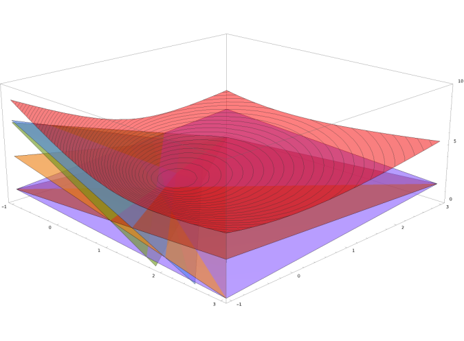
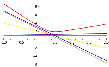
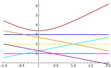
Figure 1: A plot depicting the situation of Example 1. For $c=\left(\begin{smallmatrix}1\\ 1\end{smallmatrix}\right)$, we plot a number function $c^{\top}\phi^{\theta}$, with $\theta$ consistent with the data. Any of these functions could be the unknown function. The least squares estimate is shown in yellow. If we are interested in bounds on $\hat{\phi}$, we can employ $g_{c}(z;\Theta)$ (shown in red). In particular note that this is not a linear map. Below the plot, we show the slices $z_{1}=z_{2}$ and $z_{1}=-z_{2}$ respectively.

3.2 Uncertainty on function values

The results in Section 3.1 allow us to find bounds for the unknown function $\hat{\phi}$, but do not consider how much these bounds deviate from its true value. For this, note that the result of Theorem 3.6 can be interpreted as quantifying the distance between the true function value and the least-squares estimate $\phi^{\operatorname{lse}}$ (defined in Remark 2.2) in terms of the basis functions and the data. This observation leads us to define the uncertainty corresponding to (6) at $z$ by

$$U(z;\Theta) :=\sup_{\theta\in\Theta}\|\phi^{\theta}(z)-\phi^{\operatorname{lse}}(z;\Theta)\|_{2},$$ (18a)

$$U_{c}(z;\Theta) :=\sup_{\theta\in\Theta}c^{\top}\big{(}\phi^{\theta}(z)-\phi^{\operatorname{lse}}(z;\Theta)\big{)}.$$ (18b)

Thus, if the uncertainty $U(z;\Theta)$ at $z$ is small, then $\phi^{\operatorname{lse}}(z;\Theta)$ is quantifiably a good estimate of $\hat{\phi}(z)$.

The uncertainty also allows us describe a useful variant to Problem 1(ii). In order to balance the demands of a low upper bound on the value of the true function with an associated low uncertainty, it is reasonable to consider the following generalization of the cautious suboptimization problem in (7): for $\lambda\geqslant 0$, consider

$$\min_{z\in\mathcal{S}}g(z;\Theta)+\lambda U(z;\Theta),$$ (19a)

$$\min_{z\in\mathcal{S}}g_{c}(z;\Theta)+\lambda U_{c}(z;\Theta).$$ (19b)

The following result provides a closed-form expression for the objective function in (19a).

Lemma 3.8.

(Explicit expression of uncertainty in norms) Given data $(Y,\Phi)$, let $\Theta=\mathcal{Z}(N)$, with $N$ as in (4). For $z\in\mathbb{R}^{n}$, if $b(z)\in\operatorname{im}\Phi$, then

$$U(z;\Theta)=\sqrt{\lambda_{\operatorname{max}}(N|N_{22})b(z)^{\top}(-N_{22}^{\dagger})b(z)}.$$ (20)

If $b(z)\not\in\operatorname{im}\Phi$, then $U(z;\Theta)=\infty$.

First suppose that $N$ has at least one positive eigenvalue. Similar to the proof of Lemma 3.1, we can conclude that that $\|\phi^{\theta}(z)-\phi^{\operatorname{lse}}(z;\Theta)\|_{2}\leqslant\varepsilon$ for $\varepsilon\geqslant 0$ and for all $\theta\in\Theta$ if and only if there exists $\alpha\geqslant 0$ such that

$$\begin{bmatrix}\varepsilon^{2}I&0\\ 0&-b(z)b(z)^{\top}\end{bmatrix}-\alpha\begin{bmatrix}N|N_{22}&0\\ 0&N_{22}\end{bmatrix}\geqslant 0.$$ (21)

Thus, in line with Corollary 3.2, we obtain

$$U(z;\Theta)=\min\{\varepsilon\geqslant 0\mid\exists\alpha\geqslant 0\textrm{ s.t. }\eqref{eq:LMI lse thing}\}.$$ (22)

If $b(z)\in\operatorname{im}\Phi$ then we can minimize $\varepsilon$ by taking $\alpha=b(z)^{\top}(-N_{22}^{\dagger})b(z)$, leading to (20). If $N$ does not have at least one positive eigenvalue, then $N|N_{22}=0$. As in Remark 3.3, we can conclude (22) with an inequality instead. Moreover, it immediately follows that $U(z;\Theta)\leqslant 0$, proving that (20) holds. The second part of the statement can be concluded in a similar fashion as the last part of the proof of Theorem 3.6. $\blacksquare$ In addition to expressing the uncertainty, this result also gives rise to a useful explicit bound on the function $g(z;\Theta)$.

Corollary 3.9.

(Explicit upper bound of the worst-case norm bound) Given data $(Y,\Phi)$, let $\Theta=\mathcal{Z}(N)$, with $N$ as in (4). For $z\in\mathbb{R}^{n}$, if $b(z)\in\operatorname{im}\Phi$, then

$$\begin{split}g(z;\Theta)&\leqslant\|\phi^{\operatorname{lse}}(z;\Theta)\|_{2}\\ &\quad+\sqrt{\lambda_{\operatorname{max}}(N|N_{22})b(z)^{\top}(-N_{22}^{\dagger})b(z)}.\end{split}$$ (23)

The following result provides a closed-form expression for the objective function in (19b).

Lemma 3.10.

(Explicit expression of scalar uncertainty) Given data $(Y,\Phi)$, let $\Theta=\mathcal{Z}(N)$, with $N$ as in (4). Let $z\in\mathbb{R}^{n}$ and $c\in\mathbb{R}^{m}$. If $b(z)\in\operatorname{im}\Phi$ or $c=0$, then

$$U_{c}(z;\Theta)=\sqrt{(c^{\top}(N|N_{22})c)(b(z)^{\top}(-N_{22}^{\dagger})b(z))}.$$

If $b(z)\not\in\operatorname{im}\Phi$ and $c\neq 0$, then $U_{c}(z;\Theta)=\infty$. Regardless, if $\lambda\geqslant 0$ and we define

$$\vspace{-0.3em}N_{\lambda}:=\begin{bmatrix}N_{11}&N_{12}\\ N_{21}&N_{22}\end{bmatrix}+\begin{bmatrix}\lambda(2+\lambda)(N|N_{22})&0\\ 0&0\end{bmatrix},$$

then $g_{c}(z;\Theta)+\lambda U_{c}(z;\Theta)=g_{c}(z;\mathcal{Z}(N_{\lambda}))$.

The first part follows immediately from Theorem 3.6. Now note that

$$\vspace{-0.3em}N_{\lambda}=\begin{bmatrix}(1+\lambda)^{2}(N|N_{22})+N_{12}N_{22}^{-1}N_{21}&N_{12}\\ N_{21}&N_{22}\end{bmatrix}.$$

Therefore $N_{\lambda}|N_{22}=(1+\lambda)^{2}(N|N_{22})$. Thus, the result follows from the application of Theorem 3.6. $\blacksquare$ Lemma 3.10 means that, even though problem (19b) is more general than the corresponding cautious suboptimization problem in (7), both problems can be resolved in the same fashion.

3.3 Convexity and suboptimization

In order to resolve the one-shot cautious suboptimization problem efficiently, cf. Problem 1(ii), we investigate conditions under which $g(\cdot;\Theta)$ and $g_{c}(z;\Theta)$ are convex. Towards this, we first investigate conditions under which we can guarantee that the true function $\hat{\phi}$ is convex. Since, nonnegative combinations of convex functions are convex, we provide conditions that ensure the set of parameters consistent with the measurements are nonnegative.

Lemma 3.11.

(Nonnegativity of parameters) Given data $(Y,\Phi)$, let $\Theta=\mathcal{Z}(N)$, with $N$ is as in (4). Let $c\neq 0$. Then, $\theta c\in\mathbb{R}^{k}_{\geqslant 0}$ for all $\theta\in\Theta$ if and only if $\Phi$ has full row rank and one of the following conditions hold

1. $c^{\top}(N|N_{22})c=0$ and $-N_{22}^{-1}N_{21}c\in\mathbb{R}^{k}_{\geqslant 0}$, or

2. $c^{\top}(N|N_{22})c>0$, $-N_{22}^{-1}N_{21}c\in\mathbb{R}^{k}_{>0}$ and for all $i=1,\ldots,k$,

   $$\vspace{-0.3em}c^{\top}(N|N_{22})c+\frac{(e_{i}^{\top}N_{22}^{-1}N_{21}c)^{2}}{e_{i}^{\top}N_{22}^{-1}e_{i}}\leqslant 0.$$

Recall the definition of $N_{c}$ from (14). Since $c\neq 0$ we have that $\mathcal{Z}(N)c=\mathcal{Z}(N_{c})$. Thus, $\theta c\in\mathbb{R}^{k}_{\geqslant 0}$ for all $\theta\in\Theta$ if and only if $\mathcal{Z}(N_{c})\subseteq\mathbb{R}^{k}_{\geqslant 0}$. Suppose that $\mathcal{Z}(N_{c})\subseteq\mathbb{R}^{k}_{\geqslant 0}$. This implies that the set $\mathcal{Z}(N_{c})$ contains no subspace, which implies that $N_{22}<0$. In turn, this holds if and only if $\Phi$ has full row rank.

To complete the proof, we prove that if $\Phi$ has full row rank, then $\mathcal{Z}(N_{c})\subseteq\mathbb{R}^{k}_{\geqslant 0}$ if and only if either (i) or (ii) holds. If $c^{\top}(N|N_{22})c=0$, then $N_{c}\leqslant 0$. As such, $\mathcal{Z}(N_{c})=\{-N_{22}^{-1}N_{21}\}$, that is, only the least-squares estimate is compatible with the data. The first part of the proof then follows immediately.

Next, consider $c^{\top}(N|N_{22})c>0$, that is, $N_{c}$ has one positive eigenvalue. Note that the Slater condition holds, and we can apply the S-Lemma [38, Thm 2.2] to see that $\mathcal{Z}(N_{c})\subseteq\mathbb{R}^{k}_{\geqslant 0}$ is equivalent to the existence of $\alpha_{1},\ldots,\alpha_{k}\geqslant 0$ such that

$$\vspace{-0.3em}\begin{bmatrix}0&e_{i}^{\top}\\ e_{i}&0\end{bmatrix}-\alpha_{i}N_{c}\geqslant 0,$$

for each standard basis vector $e_{i}$. This requires $\alpha_{i}\neq 0$ for each $i\in\{1,\dots,k\}$. Thus, this can equivalently written as

$$N_{c}-\frac{1}{\alpha_{i}}\begin{bmatrix}0&e_{i}^{\top}\\ e_{i}&0\end{bmatrix}\leqslant 0.$$

Since $N_{22}<0$, we can define $\beta_{i}=\tfrac{1}{\alpha_{i}}$ and conclude that the latter holds if and only if

$$c^{\top}N_{11}c-(c^{\top}N_{12}-\beta_{i}e_{i}^{\top})N_{22}^{-1}(N_{21}c-\beta_{i}e_{i})$$

$$\quad=c^{\top}(N|N_{22})c+\beta_{i}(c^{\top}N_{12}N_{22}^{-1}e_{i}+e_{i}^{\top}N_{22}^{-1}N_{21}c)$$

$$\qquad-\beta_{i}^{2}e_{i}^{\top}N_{22}^{-1}e_{i}\leqslant 0.$$

In turn, there exist such $\beta_{i}$ if and only if the minimal value over all $\beta_{i}>0$ satisfies this. Since this is a scalar expression, we can explicitly minimize it to prove the statement. $\blacksquare$

Now we can apply this result to identify conditions that ensure the convexity of $\hat{\phi}$ and its upper bound.

Corollary 3.12.

(Convexity of the true function) Given data $(Y,\Phi)$, let $\Theta=\mathcal{Z}(N)$, with $N$ is as in (4). Assume the basis functions $\phi_{i}$ are convex. Let $c\neq 0$ with $\theta c\in\mathbb{R}^{k}_{\geqslant 0}$ for all $\theta\in\Theta$. Then,

• $c^{\top}\phi^{\theta}$ is convex for all $\theta\in\Theta$ and $g_{c}(\cdot;\Theta)$ is a finite-valued convex function;

• If, in addition, the functions $\phi_{i}$ are strictly convex and $0\not\in\mathcal{Z}(N_{c})$, then $c^{\top}\phi^{\theta}$ is strictly convex for all $\theta\in\Theta$ and $g_{c}(\cdot;\Theta)$ is strictly convex.

Moreover, $\|\phi^{\theta}(\cdot)\|_{2}$ is convex if $e_{i}^{\top}\phi^{\theta}$ is convex and nonnegative for all $i=1,\ldots m$.

Lemma 3.11 shows that, if $\theta c\in\mathbb{R}^{k}_{\geqslant 0}$ for all $\theta\in\Theta$, then $\Phi$ has full row rank or, equivalently, $N_{22}<0$. This implies, cf. Remark 2.1, that $\mathcal{Z}(N)$ is compact and therefore $g_{c}(\cdot;\Theta)$ is finite-valued. The first result now follows from the facts that nonnegative combinations of convex functions are convex and that the maximum of any number of convex functions is also convex. The last part follows from standard composition rules for convexity, see e.g., [39, Example 3.14]. $\blacksquare$ Note that $0\in\mathcal{Z}(N_{c})$ if and only if $c^{\top}N_{11}c\geqslant 0$. Equivalently, this means that $Y^{\top}c\in\mathcal{Z}(\Pi_{c})$, where $\Pi_{c}$ is defined analogously to (14). This condition is easy to check in terms of data. Lemma 3.11 and Corollary 3.12 taken together mean that, if the basis functions are convex, we can test for convexity on the basis of data.

Looking back at Example 1, we can make two interesting observations. First, the conditions of Corollary 3.12 do not hold in the example, since for instance $\theta^{\operatorname{lse}}c\in\mathbb{R}^{3}_{\geqslant 0}$ only if $c=0$. Yet $c^{\top}\phi^{\theta}$ is convex for all $\theta\in\Theta$. This is because the basis functions $\phi_{i}$ are linear, and therefore the coefficients $\theta_{i}$ are not required to be nonnegative. Second, $g_{c}(\cdot;\Theta)$ in Example 1 is strictly convex for $c\neq 0$ even though the basis functions are not. Recall that we are interested in the optimization problem (7), and thus not necessarily in properties of the true function $\hat{\phi}$, but of the worst-case linear bound $g_{c}(\cdot;\Theta)$. These observations motivate our ensuing discussion to provide conditions for convexity of the upper bound instead. Under the assumptions of Theorem 3.6:

$$g_{c}(z;\Theta)=c^{\top}\phi^{\operatorname{lse}}(z;\Theta)+U_{c}(z;\Theta).$$

Thus, if (i) $c^{\top}\phi^{\operatorname{lse}}=-c^{\top}N_{12}N_{22}^{\dagger}b(\cdot)$ is convex and (ii) $U_{c}$ is convex, then so is $g_{c}$. Moreover, if in addition either is strictly convex, then so is $g_{c}$. Condition (i) can be checked directly if all basis functions $\phi_{i}$ are twice continuously differentiable by computing the Hessian of $c^{\top}\phi^{\operatorname{lse}}$. Here, we present a simple criterion, also derived from composition rules for convexity (again, see e.g., [39, Example 3.14]), to test for condition (ii).

Corollary 3.13.

(Convexity of the uncertainties) Given data $(Y,\Phi)$, let $\Theta=\mathcal{Z}(N)$ and assume $N_{22}<0$. Then both $U(\cdot;\Theta)$ and $U_{c}(\cdot;\Theta)$ are convex if each basis function $\phi_{i}$ is convex and $-N_{22}^{-1}b(z)\geqslant 0$ for all $z\in\mathbb{R}^{n}$.

In addition to guaranteeing that $g_{c}(\cdot;\Theta)$ is convex, this result can be used to find a convex upper bound when optimizing the norm, by bounding $g(\cdot;\Theta)$ using Corollary 3.9.

Equipped with the results of this section, one can solve the cautious suboptimization problems (7) efficiently. Under the assumptions of Theorem 3.6, we can write a closed-form expression for the function $g_{c}(\cdot;\Theta)$. This, in turn, allows us to test for (strict) convexity using e.g., Corollaries 3.12 or 3.13. If so, we can apply (projected) gradient descent for the optimization. For this, let $f:\mathbb{R}^{n}\rightarrow\mathbb{R}^{m}$ be differentiable, and denote its Jacobian by

$$J(f):=\begin{bmatrix}\tfrac{df}{dz_{1}}&\cdots&\tfrac{df}{dz_{n}}\end{bmatrix}=\scriptsize{\begin{bmatrix}\tfrac{df_{1}}{dz_{1}}&\cdots&\tfrac{df_{1}}{dz_{n}}\\ \vdots&&\vdots\\ \tfrac{df_{m}}{dz_{1}}&\cdots&\tfrac{df_{m}}{dz_{n}}\end{bmatrix}}.$$

Clearly, $J(\phi^{\theta})=\theta^{\top}J(b)$. The following result, consequence of Theorem 3.6, provides an expression for the Jacobian of the worst-case linear bound function.

Corollary 3.14.

(Jacobians of the worst-case linear bound) Given data $(Y,\Phi)$, let $\Theta=\mathcal{Z}(N)$ and assume $N_{22}<0$. Let the basis functions $\phi_{i}(z)$ be differentiable and such that $b(z)\neq 0$ for all $z$. Then

$$\begin{split}&J(g_{c}(z;\Theta))=\\ &\bigg{(}\!c^{\top}N_{12}+\frac{\sqrt{c^{\top}(N|N_{22})c}}{\sqrt{b(z)^{\!\top}(-N_{22}^{-1})b(z)}}b(z)^{\!\top}\bigg{)}(-N_{22}^{-1})J(b(z)).\end{split}$$

In a similar fashion, we can also obtain gradients of the bound of $g(z;\Theta)$ given in (23). Note that, if $N_{22}<0$ this requires that both $b(z)\neq 0$ and $\phi^{\operatorname{lse}}(z;\Theta)\neq 0$ for all $z$.

3.4 Set-wise verification of suboptimality

Here we solve Problem 1(iii) and provide upper (and lower) bounds as in (5) which are guaranteed to hold for all $z\in\mathcal{S}\subseteq\mathbb{R}^{n}$. In terms of $g$ and $g_{c}$, this holds only if (8) holds.

Note that $g_{-c}(z;\Theta)=-g_{c}(z;\Theta)$, and therefore $g_{c}(z;\Theta)$ is concave if and only if $g_{-c}(\cdot;\Theta)$ is convex. Moreover,

$$\max_{z\in\mathcal{S}}g_{c}(z;\Theta)=-\min_{z\in\mathcal{S}}g_{-c}(z;\Theta).$$

Therefore, we can test for concavity of $g_{c}$ and apply the minimization results to $g_{-c}$ of the Section 3.3. Beyond the case of concavity, we can also employ convexity in order to efficiently provide upper bounds over the convex hull of a finite set, as the following result shows.

Proposition 3.15.

(Convexity and maximal values) Given data $(Y,\Phi)$, let $\Theta=\mathcal{Z}(N)$. Let $\mathcal{F}\subseteq\mathbb{R}^{n}$ be a finite set and let $\mathcal{S}=\operatorname{conv}\mathcal{F}$. Suppose that $g(z;\Theta)$ is convex. Then (9) for all $z\in\mathcal{S}$ if and only if

$$g(z;\Theta)\leqslant\delta\quad\forall z\in\mathcal{F}.$$

Similarly, if $g_{c}(z;\Theta)$ is convex, then (15) for all $z\in\mathcal{S}$ if and only if

$$g_{c}(z;\Theta)\leqslant\delta\quad\forall z\in\mathcal{F}.$$

The proof of this result follows immediately from the fact that any convex function attains its maximum over $\mathcal{S}$ on $\mathcal{F}$. Thus, convexity (resp., concavity) allows us to find minimal upper bounds (resp., maximal lower bounds) over a set, leading to a solution of Problem 1.(iii). In order to provide bounds over sets in scenarios where convexity or concavity cannot be guaranteed, we investigate Lipschitz continuity. This leads to conditions that can be checked at a finite number of points. Therefore, we are first interested in the question whether for all $z,z^{\star}\in\mathcal{S}\subseteq\mathbb{R}^{n}$, it holds that

$$\|\hat{\phi}(z)-\hat{\phi}(z^{\star})\|_{2}\leqslant L\|z-z^{\star}\|_{2}.\vspace{-0.2em}$$

More generally, and for later reference, the following result considers the more general case of weighted norms.

Lemma 3.16.

(Lipschitz constants of functions consistent with the measurements) Given data $(Y,\Phi)$, let $\Theta=\mathcal{Z}(N)$, with $N$ as in (4), and assume $N$ has at least one positive eigenvalue. Let $P\in\mathbb{S}^{m}$ and $Q\in\mathbb{S}^{n}$ with $P>0$ and $Q>0$. For $L\geqslant 0$ and $z,z^{\star}\in\mathcal{S}\subseteq\mathbb{R}^{n}$, we have

$$\|\phi^{\theta}(z)-\phi^{\theta}(z^{\star})\|_{2,P^{1/2}}\leqslant L\|z-z^{\star}\|_{2,Q^{1/2}}\quad\textrm{ for all }\quad\theta\in\Theta$$

if and only if there exists $\alpha\geqslant 0$ such that

$$\scriptsize{\left[\vbox{\hbox{\kern-1.1563pt\raise 0.0pt\hbox{\kern 60.33533pt}\kern 0.0pt\vbox{}\kern-1.1563pt}}\right]}-\alpha\normalsize{\left[\vbox{\hbox{\kern-1.1563pt\raise 0.0pt\hbox{\kern 14.12498pt}\kern 0.0pt\vbox{}\kern-1.1563pt}}\right]}\geqslant 0.\vspace{-0.3em}$$ (24)

If, in addition the basis functions $\phi_{i}$ are differentiable, then

$$\vspace{-0.2em}\|J(\phi^{\theta})\|_{2}\leqslant L\quad\textrm{ for all }\quad\theta\in\Theta$$

if and only if there exists $\alpha\geqslant 0$ such that

$$\vspace{-0.2em}\scriptsize{\left[\vbox{\hbox{\kern-1.1563pt\raise 0.0pt\hbox{\kern 42.84792pt}\kern 0.0pt\vbox{}\kern-1.1563pt}}\right]-\normalsize{\alpha\left[\vbox{\hbox{\kern-1.1563pt\raise 0.0pt\hbox{\kern 14.12498pt}\kern 0.0pt\vbox{}\kern-1.1563pt}}\right]}\geqslant 0.}$$ (25)

Note that $\phi^{\theta}(z)-\phi^{\theta}(z^{\star})=\theta^{\top}(b(z)-b(z^{\star}))$. Similarly, $J(\phi^{\theta})=\theta^{\top}J(b)$. The result can then be proven by following the steps of the proof of Lemma 3.1. $\blacksquare$

Remark 3.17.

(Single check for establishing Lipschitz constant) To check for Lipschitzness, we can employ the method of Remark 3.4 to avoid checking (24) for all $z,z^{\star}\in\mathbb{R}^{n}$. Suppose the basis satisfies a Lipschitz condition of the form

$$\|b(z)-b(z^{\star})\|_{2}\leqslant L_{b}\|z-z^{\star}\|^{2}_{2,Q^{1/2}},$$

for all $z,z^{\star}\in\mathbb{R}^{n}$. Then,

$$\vspace{-0.2em}\frac{(b(z)-b(z^{\star}))(b(z)-b(z^{\star}))^{\top}}{\|z-z^{\star}\|^{2}_{2,Q^{1/2}}}\leqslant L_{b}^{2}I,\vspace{-0.2em}$$

and thus, as in Remark 3.4 we have

$$\scriptsize{\begin{bmatrix}L^{2}P^{-1}&0\\ 0&-L_{b}^{2}I_{k}\end{bmatrix}}-\normalsize{\alpha N\geqslant 0}$$ (26)

implies (24). This gives a single condition to check to establish a Lipschitz constant valid for all $z,z^{\star}\in\mathbb{R}^{n}$. $\bullet$

The characterization of Lipschitz constants in terms of data in Lemma 3.16 allows us to bound the unknown function $\hat{\phi}$ as follows. To do this, we use the following notion: The set $\mathcal{G}\subset\mathbb{R}^{n}$ is an $\varepsilon$-covering of $\mathcal{S}\subseteq\mathbb{R}^{n}$ if for every $z\in\mathcal{S}$ there exists $z^{\star}\in\mathcal{G}$ such that $\|z-z^{\star}\|_{2}\leqslant\varepsilon$. If $\mathcal{S}$ is a bounded set, then for any $\varepsilon>0$, there exists an $\varepsilon$-covering with finitely many elements.

Theorem 3.18.

(Coverings and bounds) Given data $(Y,\Phi)$, let $\Theta=\mathcal{Z}(N)$. For $\varepsilon>0$, let $\mathcal{G}$ be a finite $\varepsilon$-covering of $\mathcal{S}\subseteq\mathbb{R}^{n}$. Suppose that $g(z;\Theta)$ is Lipschitz with constant $L$ on $\mathcal{S}$. Then, for all $z\in\mathcal{S}$,

$$\min_{z^{\star}\in\mathcal{G}}g(z^{\star};\Theta)-\varepsilon L\leqslant g(z;\Theta)\leqslant\max_{z^{\star}\in\mathcal{G}}g(z^{\star};\Theta)+\varepsilon L.$$

If $g_{c}(z;\Theta)$ is Lipschitz with constant $L$, then for all $z\in\mathcal{S}$,

$$\min_{z^{\star}\in\mathcal{G}}g_{c}(z^{\star};\Theta)-\varepsilon L\leqslant g_{c}(z;\Theta)\leqslant\max_{z^{\star}\in\mathcal{G}}g_{c}(z^{\star};\Theta)+\varepsilon L.$$

We omit the proof, which follows directly from combining the definitions of Lipschitz continuity and $\varepsilon-$coverings.

This result means that we can find guaranteed upper and lower bounds of either $\|\hat{\phi}(z)\|$ or $c^{\top}\hat{\phi}(z)$ over the bounded set $\mathcal{S}$ in terms of a finite number of evaluations of $g(z;\Theta)$ or $g_{c}(z;\Theta)$, resp. In turn, recall that Corollary 3.2 allows us to efficiently find function values of $g(z;\Theta)$ on the basis of measurements and, similarly, Theorem 3.6 allows us to directly calculate values of $g_{c}(z;\Theta)$.

4 Applications to system analysis and control

In this section, we exploit the proposed solutions to Problem 1 in two applications: contraction analysis of unknown nonlinear systems and regulation of an unknown linear system to a suboptimal point of an unknown cost function.

4.1 Data-based contraction analysis for nonlinear systems

Consider the autonomous discrete- or continuous-time system given by either

$$z_{k+1}=\hat{\phi}(z_{k}),\textrm{ or}\quad\dot{z}(t)=\hat{\phi}(z(t)),\vspace{-0.3em}$$ (27)

where $\hat{\phi}:\mathbb{R}^{n}\rightarrow\mathbb{R}^{n}$ is an unknown function. We consider noisy measurements (2) as described in Section 2. Therefore $\hat{\phi}=\phi^{\theta}$ for some $\theta\in\Theta=\mathcal{Z}(N)$. In the continuous-time case, this means that we collect noisy measurements of the derivative of the state at a finite set of states (see [27] for a discussion on this assumption).

The discrete-time system in (27) is strongly contracting (cf. [29, Sec. 3.4]) with respect to the weighted norm $\|\cdot\|_{2,P^{1/2}}$ if $\hat{\phi}$ admits a Lipschitz constant $L<1$, that is,

$$\|\hat{\phi}(z)-\hat{\phi}(z^{\star})\|_{2,P^{1/2}}\leqslant L\|z-z^{\star}\|_{2,P^{1/2}}.$$

One can now directly employ Lemma 3.16 in order to obtain data-based conditions under which this property holds.

To deal with the situation of continuous-time systems, we first require a number of prerequisites. Given $P>0$, a function $f:\mathbb{R}^{n}\rightarrow\mathbb{R}^{n}$ is one-sided Lipschitz with respect to $\|\cdot\|_{2,P^{1/2}}$ if there exists $\gamma\in\mathbb{R}$ such that, for all $z,z^{\star}\in\mathbb{R}^{n}$,

$$(z-z^{\star})^{\top}P(f(z)-f(z^{\star}))\leqslant\gamma\|z-z^{\star}\|^{2}_{2,P^{1/2}}.\vspace{-0.3em}$$ (28)

Such $\gamma$ is called a one-sided Lipschitz constant and the smallest such $\gamma$ is denoted $\operatorname{osLip}(f)$. The autonomous system $\dot{z}(t)=f(z(t))$ is strictly contracting with rate $|b|$ if $\operatorname{osLip}(f)\leqslant b<0$. Given any two trajectories $x(t),\bar{x}(t)$ of a stricly contracting system, one has $\|x(t)-\bar{x}(t)\|_{2,P^{1/2}}\leqslant e^{b(t-s)}\|x(s)-\bar{x}(s)\|_{2,P^{1/2}}$ for any $t\geqslant s\geqslant 0$.

The following result, derived from Theorem 3.6, establishes a test for strict contractivity of the continuous-time system in (27) on the basis of a set of measurements of $\hat{\phi}$.

Theorem 4.1.

(Data-based test for strict contractivity) Given data $(Y,\Phi)$, let $\Theta=\mathcal{Z}(N)$, with $N$ as in (4). Let $P>0$ and $z,z^{\star}\in\mathbb{R}^{n}$. Assume $\Phi$ has full row rank. Then,

$$(z-z^{\star})^{\top}P\theta^{\top}(b(z)-b(z^{\star}))\leqslant\gamma\|z-z^{\star}\|^{2}_{2,P^{1/2}}$$

for all $\theta\in\Theta$ if and only if

$$(z-z^{\star})^{\top} P(-N_{12}N_{22}^{-1})(b(z)-b(z^{\star}))$$

$$+\sqrt{(z-z^{\star})^{\top}P(N|N_{22})P(z-z^{\star})}$$

$$\quad\cdot\sqrt{(b(z)-b(z^{\star}))^{\top}(-N_{22}^{-1})(b(z)-b(z^{\star}))}$$

$$\leqslant\gamma\|z-z^{\star}\|^{2}_{P^{1/2}}.\vspace{-0.5em}$$

As a consequence of this result, we can provide a test to establish strict contractivity in terms only of the least-squares estimate $\phi^{\operatorname{lse}}$, the data matrix $N$, and a Lipschitz constant for the basis functions.

Corollary 4.2.

(Strict contractivity in terms of the least-squares estimate) Given data $(Y,\Phi)$, let $\Theta=\mathcal{Z}(N)$, with $N$ as in (4). Assume $\Phi$ has full row rank. Let $L$ be such that $\|b(z)-b(z^{\star})\|_{2,(-N_{22})^{-1/2}}\leqslant L\|z-z^{\star}\|_{2}$, for all $z,z^{\star}\in\mathbb{R}^{n}$. Then, for $P>0$,

$$(z-z^{\star})^{\top}P\theta^{\top}(b(z)-b(z^{\star}))\leqslant\gamma\|z-z^{\star}\|^{2}_{2,P^{1/2}}$$

for all $\theta\in\Theta$ and $z,z^{\star}\in\mathbb{R}^{n}$ if

$$\operatorname{osLip}(\phi^{\operatorname{lse}})<\gamma-L\sqrt{\lambda_{\textup{max}}(N|N_{22})}\frac{\lambda_{\textup{max}}(P)}{\lambda_{\textup{min}}(P)}.\vspace{-0.3em}$$ (29)

Remark 4.3.

(Contraction w.r.t. different norms) The results of this section can be readily generalized to contractivity (and thus one-sided Lipschitzness) with respect to $\|\cdot\|_{p,R}$ for $p\in[1,\infty)$. To do this, one replaces the one-sided Lipschitz condition (28) with the respective condition from [40, Table I] and adjust the statements accordingly. Note that the case of $\|\cdot\|_{\infty,R}$ is not amenable to this treatment because the corresponding one-sided Lipschitz condition $\operatorname{osLip}(f)$ is not linear in $f$. $\bullet$

4.2 Suboptimal regulation of unknown systems

Consider the problem of regulating an unknown linear system to a suboptimal point of the norm of an unknown cost function $\hat{\phi}:\mathbb{R}^{n}\rightarrow\mathbb{R}^{m}$ on the basis of measurements. We consider noisy measurements (2) as described in Section 2. In short, $\hat{\phi}=\phi^{\theta}$ for some $\theta\in\Theta=\mathcal{Z}(N)$. Moreover, let

$$x_{k+1}=\hat{A}x_{k}+\hat{B}u_{k},$$

with state $x_{k}\in\mathbb{R}^{n}$ and input $u_{k}\in\mathbb{R}^{r}$. Here, $\hat{A}\in\mathbb{R}^{n\times n}$ and $\hat{B}\in\mathbb{R}^{n\times r}$. If $\hat{A}$ is stable, we know that any fixed point corresponds to a constant input $u^{\star}$. Indeed, if we apply the constant input $u_{k}=u^{\star}$, no matter the initial condition $x_{0}$, the state asymptotically converges to the fixed point

$$\vspace{-0.3em}\lim_{k\rightarrow\infty}x_{k}=x^{\star}:=(I\!-\!\hat{A})^{-1}\hat{B}u^{\star}.$$

This means that we can find a static input to regulate the system towards any state in $\operatorname{im}(I\!-\!\hat{A})^{-1}\hat{B}\subseteq\mathbb{R}^{n}$.

We are interested in regulating the state to a point $x^{\star}$ for which we can guarantee that $\|\hat{\phi}(x^{\star})\|_{2}\leqslant\delta$, with a value of $\delta$ as small as possible. If $\hat{A}$ and $\hat{B}$ are known, this corresponds to Problem 1(ii) with $\mathcal{S}=\operatorname{im}(I\!-\!\hat{A})^{-1}\hat{B}$.

Now assume that we do not have access to the matrices $\hat{A}$ and $\hat{B}$. Instead, we assume that we have not only measurements of $\hat{\phi}$, but additionally a set of noisy measurements corresponding to the unknown system. To be precise, we collect measurements of the system

$$x_{k+1}=\hat{A}x_{k}+\hat{B}u_{k}+w_{k}.$$ (30)

Using the basis functions

$$\psi_{i}(x,u)=\begin{cases}x_{i}&\textrm{ for }i=1,\ldots,n\\ u_{i}&\textrm{ for }i=n+1,\ldots n+r,\end{cases}$$

and collecting measurements of the state and input signals reduces the setup of Section 2 to that of e.g., [37]. To avoid some unnecessary repetition, we simply state here that on the basis of measurements, we can conclude that $(A,B)^{\top}\in\Sigma=\mathcal{Z}(M)$, where $M\in\mathbb{S}^{n+(n+r)}$ is analogous to $N$ in (4).

In order to be able to regulate the unknown system in the same manner as before, recall that we require that $\hat{A}$ is stable. Given that, on the basis of measurements we can not distinguish $\hat{A}$ from other matrices $A$ such that $(A,B)^{\top}\in\Sigma$, we therefore require all such $A$ to be stable. In the following, we describe a test for the existence of a shared quadratic Lyapunov function, which is a stronger stability condition. For a detailed discussion on the conservativeness of this assumption, see e.g., [41]. Now we can easily adapt e.g., [37, Thm. 5.1] to obtain the following.

Lemma 4.4 (Informativity for stability).

Let $\Sigma=\mathcal{Z}(M)$, where the corresponding noise model satisfies Assumption 1. Then, there exists $P\in\mathbb{S}^{n}$ with $P>0$ and $APA^{\top}<P$ for all $(A,B)^{\top}\in\Sigma$ if and only if there exist $\bar{P}\in\mathbb{S}^{n}$ with $\bar{P}>0$ and $\beta>0$ such that

$$\scriptsize{\left[\vbox{\hbox{\kern-1.1563pt\raise 0.0pt\hbox{\kern 29.6609pt}\kern 0.0pt\vbox{}\kern-1.1563pt}}\right]}\normalsize{-M\geqslant 0}.$$ (31)

Remark 4.5.

(Stability and contractivity) Applying a fixed input $u^{\star}$ to the unknown system yields an autonomous discrete-time system. We know that for any initial condition $x_{0}$, this system converges to a fixed point. Moreover, if $P>0$ and $APA^{\top}<P$ for all $(A,B)^{\top}\in\Sigma$, then $A^{\top}P^{-1}A<P^{-1}$. Therefore, one can see that the system is strongly contracting with respect to $\|\cdot\|_{2,P^{-1/2}}$. $\bullet$

When each system matrix $A$ in the set $\Sigma$ of systems consistent with the data is stable, we can characterize the fixed points resulting from applying the same input to each.

Lemma 4.6 (Characterizing fixed points).

Let $\Sigma=\mathcal{Z}(M)$, where the corresponding noise model satisfies Assumption 1 and $M$ has at least one positive eigenvalue. Assume $A$ is stable for all $(A,B)^{\top}\in\Sigma$. Given $x\in\mathbb{R}^{n}$ and $u\in\mathbb{R}^{r}$, $\|x-(I\!-\!A)^{-1}Bu\|_{2}\leqslant\varepsilon$ for all $(A,B)^{\top}\in\Sigma$ if and only if there exists $\gamma\geqslant 0$ such that

$$\scriptsize\left[\vbox{\hbox{\kern-1.1563pt\raise 0.0pt\hbox{\kern 39.64764pt}\kern 0.0pt\vbox{}\kern-1.1563pt}}\right]\normalsize-\gamma\left[\vbox{\hbox{\kern-1.1563pt\raise 0.0pt\hbox{\kern 15.79167pt}\kern 0.0pt\vbox{}\kern-1.1563pt}}\right]\geqslant 0\vspace{-0.4em}$$ (32)

Let $(A,B)^{\top}\in\Sigma$. First, note that we have

$$\qquad\|x-(I_{n}\!-\!A)^{-1}Bu\|_{2}\leqslant\varepsilon$$

$$\Leftrightarrow(x-(I_{n}\!-\!A)^{-1}Bu)(x-(I_{n}\!-\!A)^{-1}Bu)^{\top}\leqslant\varepsilon^{2}I.\vspace{-0.3em}$$

Since $A$ is stable, we know that $I-A$ is nonsingular. Thus, the previous holds if and only if

$$\vspace{-0.3em}((I\!-\!A)x-Bu)((I\!-\!A)x-Bu)^{\top}\!\leqslant\varepsilon^{2}(I\!-\!A)(I\!-\!A)^{\top},$$

or equivalently,

$$\vspace{-0.3em}\scriptsize\begin{bmatrix}I_{n}\\ A^{\top}\\ B^{\top}\end{bmatrix}^{\!\top}\!\!\left(\begin{bmatrix}\varepsilon^{2}I_{n}&-\varepsilon^{2}I_{n}\!&0\\ -\varepsilon^{2}I_{n}&\varepsilon^{2}I_{n}&0\\ 0&0&0\end{bmatrix}\!-\!\begin{pmatrix}x\\ -x\\ -u\end{pmatrix}\!\!\!\begin{pmatrix}x\\ -x\\ -u\end{pmatrix}^{\!\!\top}\right)\!\!\begin{bmatrix}I_{n}\\ A^{\top}\\ B^{\top}\end{bmatrix}\geqslant 0.$$

As such, the set of $(A,B)$ that satisfy the condition can be written as the solution set of a QMI. By assumption $\Sigma=\mathcal{Z}(M)$. We can then apply the matrix S-Lemma [37, Thm 4.7] and use a Schur complement to prove the statement. $\blacksquare$ Motivated by Lemma 4.6, we define

$$\varepsilon^{-}(x):=\min\{\varepsilon\mid\exists\gamma\geqslant 0,u\in\mathbb{R}^{r}\textrm{ s.t. }\eqref{eq:LMI bd i-o}\textrm{ holds}\}.$$ (33)

Given $x\in\mathbb{R}^{N}$, the function $\varepsilon^{-}(x)$ thus gives the minimal radius of a ball around $x$, for which there exists a $u^{\star}$ such that the corresponding set of fixed points of each system in $\Sigma$ is contained in this ball. The next result describes useful properties of this function.

Lemma 4.7.

(Properties of the minimal radius function) Let $\Sigma=\mathcal{Z}(M)$, where the corresponding noise model satisfies Assumption 1 and $M$ has at least one positive eigenvalue. Assume $A$ is stable for all $(A,B)^{\top}\in\Sigma$. Then $\varepsilon^{-}(x)\leqslant\|x\|_{2}$ for any $x\in\mathbb{R}^{n}$ and $\varepsilon^{-}$ is convex.

The statement $\varepsilon^{-}(x)\leqslant\|x\|_{2}$ follows by noting that, for any $x$ and $M$, (32) holds with $u=0$, $\gamma=0$ and $\varepsilon=\|x\|_{2}$. Next, suppose that for all $(A,B)^{\top}\in\Sigma$,

$$\|x-(I\!-\!A)^{-1}Bu\|_{2}\leqslant\varepsilon,\quad\|\bar{x}-(I\!-\!A)^{-1}B\bar{u}\|_{2}\leqslant\bar{\varepsilon}.$$

Let $\lambda\in[0,1]$ and define $x_{\lambda}:=\lambda x+(1-\lambda)\bar{x}$ and similarly for $u_{\lambda}$ and $\varepsilon_{\lambda}$. Then,

$$\|x_{\lambda}-(I\!-\!A)^{-1}Bu_{\lambda}\|_{2}\leqslant\lambda\|x-(I\!-\!A)^{-1}Bu\|_{2}$$

$$+(1-\lambda)\|\bar{x}-(I\!-\!A)^{-1}B\bar{u}\|_{2}\leqslant\varepsilon_{\lambda}.$$

Therefore, $\varepsilon^{-}(x_{\lambda})\leqslant\varepsilon_{\lambda}$, proving that $\varepsilon^{-}$ is convex in $x$. $\blacksquare$

The following result uses this function in order to provide conditions for suboptimal regulation.

Theorem 4.8.

(Suboptimal regulation) Let $\Sigma=\mathcal{Z}(M)$ and $\Theta=\mathcal{Z}(N)$, where the corresponding noise models satisfy Assumption 1. Assume $A$ is stable for all $(A,B)^{\top}\in\Sigma$ and $\phi^{\theta}$ is Lipschitz with constant $L$ for all $\theta\in\Theta$. Then

$$\min_{u}\|\hat{\phi}((I-\hat{A})^{-1}\hat{B}u)\|_{2}\leqslant\min_{x}\,\big{(}g(x;\Theta)+L\varepsilon^{-}(x)\big{)}.$$

Using the triangle inequality and Lipschitzness,

$$\|\hat{\phi}((I-\hat{A})^{-1}\hat{B}u)\|_{2}\leqslant\|\hat{\phi}(x)\|_{2}+L\|x-(I\!-\!\hat{A})^{-1}\hat{B}u\|_{2},$$

for any $x\in\mathbb{R}^{n}$. Note that this separates the unknown parameter $\hat{\theta}$ from the unknown pair $(\hat{A},\hat{B})$. From here, we deduce

$$\min_{u}\|\hat{\phi}((I-\hat{A})^{-1}\hat{B}u)\|_{2}$$

$$\leqslant\min_{x,u}\Big{(}\max_{\theta\in\Theta}\|\phi^{\theta}(x)\|+L\Big{(}\max_{(A,B)\in\Sigma}\|x-(I\!-\!A)^{-1}Bu\|\Big{)}\Big{)}.$$

Since only the second term is dependent on $u$, we can use the definition of $\varepsilon^{-}(x)$ and Lemma 4.6 to conclude the statement. $\blacksquare$

Now, since we know that $\varepsilon^{-}$ is convex, we can resolve this problem efficiently if so is $g(\cdot,\Theta)$ (see Corollary 3.13). We conclude this section by noting that Theorem 4.8 requires only stability of each system matrix $A$. Under the stronger assumption of quadratic stability, which can be determined using Lemma 4.4, we can provide a transient guarantee on the values of the unknown function.

Theorem 4.9.

(Transient values of the cost function) Let $\Sigma=\mathcal{Z}(M)$ and $\Theta=\mathcal{Z}(N)$, where the corresponding noise models satisfy Assumption 1. Let $P>0$ such that $APA^{\top}<P$ for all $(A,B)^{\top}\in\Sigma$ and assume $\phi^{\theta}$ is Lipschitz with constant $L$ for all $\theta\in\Theta$. Let $\delta>0$ and $u^{\star}$ be a fixed input such that $\|\hat{\phi}((I-\hat{A})^{-1}\hat{B}u^{\star})\|_{2}\leqslant\delta$. Given an initial condition $\hat{x}_{0}\in\mathbb{R}^{n}$, let $\hat{x}_{k}$ denote the trajectory of the unknown system $(\hat{A},\hat{B})$ corresponding to the input $u^{\star}$ and starting from $\hat{x}_{0}$. Then, there exists $\lambda\in[0,1)$ such that

$$\vspace{-0.3em}\|\hat{\phi}(\hat{x}_{k})\|_{2}\leqslant\delta+\lambda^{k}L\frac{\lambda_{\textup{max}}(P)}{\lambda_{\textup{min}}(P)}\|\hat{x}_{0}-x^{\star}\|_{2}.$$

Let $x^{\star}$ be the fixed point corresponding to the input $u^{\star}$ for the system $(\hat{A},\hat{B})$. If $APA^{\top}<P$ for all $(A,B)^{\top}\in\Sigma$, then the set $\{A\mid(A,B)^{\top}\in\Sigma\}$ is bounded. Since the set is closed by definition, we can conclude that $APA^{\top}<P$ for all $(A,B)^{\top}\in\Sigma$ if and only if there exists $\lambda\in[0,1)$ such that $APA^{\top}<\lambda P$ for all $(A,B)^{\top}\in\Sigma$. In particular, this implies that the affine system resulting from the application of input $u^{\star}$ to $(\hat{A},\hat{B})$ is strongly contracting (cf. Remark 4.5). Thus, for any $k\geqslant 1$,

$$\|\hat{x}_{k}-x^{\star}\|_{2,P^{-1/2}}\leqslant\lambda\|\hat{x}_{k-1}-x^{\star}\|_{2,P^{-1/2}}.$$

By applying this repeatedly, we conclude $\|\hat{x}_{k}-x^{\star}\|_{2,P^{-1/2}}\leqslant\lambda^{k}\|\hat{x}_{0}-x^{\star}\|_{2,P^{-1/2}}$, and thus

$$\vspace{-0.3em}\|\hat{x}_{k}-x^{\star}\|_{2}\leqslant\lambda^{k}\frac{\lambda_{\textup{max}}(P^{-1})}{\lambda_{\textup{min}}(P^{-1})}\|\hat{x}_{0}-x^{\star}\|_{2}.$$

Using the triangle inequality and the fact that $\hat{\phi}$ is Lipschitz with constant $L$,

$$\|\hat{\phi}(\hat{x}_{k})\|_{2}\leqslant\|\hat{\phi}(x^{\star})\|_{2}+L\|\hat{x}_{k}-x^{\star}\|_{2}.$$

Combining this previous with the fact that $\lambda_{\textup{max}}(P^{-1})={1}/{\lambda_{\textup{min}}(P)}$ and $\lambda_{\textup{min}}(P^{-1})={1}/{\lambda_{\textup{max}}(P)}$ yields

$$\vspace{-0.3em}\|\hat{\phi}(\hat{x}_{k})\|_{2}\leqslant\delta+\lambda^{k}L\frac{\lambda_{\textup{max}}(P)}{\lambda_{\textup{min}}(P)}\|\hat{x}_{0}-x^{\star}\|_{2}.$$

This proves the statement. $\blacksquare$

Remark 4.10.

(Suboptimal regulation of unstable systems) Our discussion above assumes that the unknown system and all of those consistent with the measurements are stable. When this is not the case, we can instead proceed by first testing if the data is sufficiently informative for quadratic stabilization, i.e., to guarantee the existence of a static feedback $K$ such that $(A+BK)P(A+BK)^{\top}<P$ for all $(A,B)^{\top}\in\Sigma$, cf [37, Thm. 5.1]. Then, we can characterize the behavior of the fixed points of the resulting systems by considering

$$\vspace{-0.3em}\|x-(I\!-\!A+BK)^{-1}Bu\|_{2}\leqslant\varepsilon.$$

Adapting Lemma 4.6 and the definition of $\varepsilon^{-}$ accordingly is then straightforward. This gives rise to a two-step approach: (i) determine a gain $K$ which stabilizes all systems in $\Sigma$ and (ii) minimize $g(x;\Theta)+L\varepsilon^{-}(x)$. Note that the choice of $K$ among potentially many stabilizing gains influences the resulting $\varepsilon^{-}$ in a nontrivial way. We leave the analysis of jointly minimizing $g(x;\Theta)+L\varepsilon^{-}(x)$ over all $x$ and all possible choices $K$ as an open problem. $\bullet$

5 Online cautious optimization

Our exposition so far has considered one-shot optimization settings where, given a set of measurements, we determine regularity properties and address suboptimization of the unknown function. In this section, we consider online scenarios, where one can repeatedly combine optimization of the unknown function with the collection of additional measurements, aiming at reducing the optimality gap. Consistent with our exposition, this means that we are interested in finding guaranteed upper bounds on $c^{\top}\hat{\phi}$ on the basis of initial measurements, then refining this bound on the basis of newly collected measurements. We aim at doing this in a monotonic fashion, that is, in a way that has the obtained upper bounds do not increase as time progresses.

Consider repeated measurements of the form

$$Y_{k}=\hat{\theta}^{\top}\Phi_{k}+W_{k},\textrm{ with }W_{k}^{\top}\in\mathcal{Z}(\Pi),$$ (34)

where $Y_{k}$ and $W_{k}$ are as in (2) and $k\in\mathbb{N}$. Let $\Theta_{k}:=\mathcal{Z}(N_{k})$ be the set of of parameters which are compatible with the $k^{\textup{th}}$ set of measurements, where

$$\vspace{-0.3em}N_{k}:=\begin{bmatrix}I&Y_{k}\\ 0&-\Phi_{k}\end{bmatrix}\Pi\begin{bmatrix}I&Y_{k}\\ 0&-\Phi_{k}\end{bmatrix}^{\top}.$$

Our online optimization strategy is described as follows.

Algorithm 1.

(Online cautious optimization) Consider an initial candidate optimizer $z_{0}\in\mathbb{R}^{n}$, an initial set of data $(Y_{0},\Phi_{0})$, and $c\in\mathbb{R}^{m}$. Define the initial set of compatible parameters as $\bar{\Theta}_{0}=\mathcal{Z}(N_{0})$, where $N_{0}$ is given as in (4). For $k\geqslant 1$, we alternate two steps:

1. Employ the set $\bar{\Theta}_{k-1}$ to improve the candidate optimizer by finding $z_{k}$ such that

   $$g_{c}(z_{k};\bar{\Theta}_{k-1})\leqslant g_{c}(z_{k-1};\bar{\Theta}_{k-1}).$$ (35)

2. Measure the function as in (34) and update the set of parameters by finding a set $\bar{\Theta}_{k}$ such that $\hat{\theta}\in\bar{\Theta}_{k}$ and

   $$g_{c}(z_{k};\bar{\Theta}_{k})\leqslant g_{c}(z_{k};\bar{\Theta}_{k-1}).$$ (36)

In the following, we enforce (36) by considering parameters consistent with all previous measurements,

$$\vspace{-0.3em}\bar{\Theta}_{k}:=\Theta_{0}\cap\ldots\cap\Theta_{k}.$$ (37)

Note that Algorithm 1 provides a sequence of upper bounds to true function values, on the basis of measurements. This means that after any number of iterations, we obtain a worst-case estimate of the function value $c^{\top}\hat{\phi}(z_{k})$ and, as such, for the minimum of $c^{\top}\hat{\phi}$. To be precise, for each $k\geqslant 1$,

$$\vspace{-0.3em}\min_{z\in\mathbb{R}^{n}}c^{\top}\hat{\phi}(z)\leqslant c^{\top}\hat{\phi}(z_{k})\leqslant g_{c}(z_{k};\bar{\Theta}_{k-1}),$$ (38)

and these bounds are monotonically nonincreasing

$$\vspace{-0.3em}g_{c}(z_{k+1};\bar{\Theta}_{k})\leqslant g_{c}(z_{k};\bar{\Theta}_{k-1})$$ (39)

Therefore this sequence of upper bounds is nonincreasing and bounded below, and we can conclude that the algorithm converges. However, without further assumptions, one cannot guarantee convergence of the upper bounds to the minimal value of $c^{\top}\hat{\phi}$, or respectively of $z_{k}$ to the global minimum of $c^{\top}\hat{\phi}$. This is because, even though when repeatedly collecting measurements, it is reasonable to assume that the set of consistent parameters would decrease in size, this is not necessarily the case in general. In particular, a situation might arise where repeated measurements corresponding to a worst-case, or adversarial, noise signal give rise to convergence to a fixed bound with nonzero uncertainty. This is the point we address next by considering random noise realizations.

5.1 Collection of uniformly distributed measurements

We consider a scenario where the noise samples are not only bounded but distributed uniformly over the set $\mathcal{Z}(\Pi)$. To formalize this, let $\Pi$ be such that $\mathcal{Z}(\Pi)$ is bounded. Consider a measure $\mu$, and probability distribution $p$,

$$p(W):=\begin{cases}\frac{1}{\mu(\mathcal{Z}(\Pi))}&W^{\top}\in\mathcal{Z}(\Pi),\\ 0&\textrm{otherwise}.\end{cases}$$

As a notational shorthand, we write $W^{\top}\sim\operatorname{Uni}(\mathcal{Z}(\Pi))$. The following result shows that, under such uniformly distributed noise samples, the size of the set of parameters indeed shrinks with increasing $k$.

Theorem 5.1.

(Repeated measurements leading to shrinking set of consistent parameters) Suppose that the measurements $(Y_{k},\Phi_{k})$ are collected such that $W_{k}^{\top}\sim\operatorname{Uni}(\mathcal{Z}(\Pi))$ and $\sigma_{-}(\Phi_{k}(z))\geqslant a$ for some $a\in\mathbb{R}_{>0}$ and all $z\in\mathbb{R}^{n}$. Then, for any probability $0<\pi<1$ and any $\varepsilon>0$, there exists $k$ such that if $B_{\varepsilon}(\hat{\theta})$ denotes the ball of radius $\varepsilon>0$ centered at $\hat{\theta}$ in $\mathbb{R}^{k\times m}$, then

$$\vspace{-0.3em}p(\Theta_{0}\cap\ldots\cap\Theta_{k-1}\subseteq B_{\varepsilon}(\hat{\theta}))>\pi.$$ (40)

Let $k\geqslant 0$ and consider the set $\Theta_{k}=\mathcal{Z}(N_{k})$. In terms of the true parameter $\hat{\theta}$, we obtain $Y_{k}=\hat{\theta}^{\top}\Phi_{k}+W_{k}$, with $W_{k}^{\top}\sim\operatorname{Uni}(\mathcal{Z}(\Pi))$. This implies that

$$\vspace{-0.3em}Y_{k}^{\top}\sim\operatorname{Uni}(\mathcal{Z}(\Pi)+\Phi_{k}^{\top}\hat{\theta}).$$

For $\theta\in\mathbb{R}^{k}$, we know that $\theta\in\Theta_{k}$ if and only if $Y_{k}^{\top}-\Phi_{k}^{\top}\theta\in\mathcal{Z}(\Pi)$. Therefore, $Y_{k}^{\top}-\Phi_{k}^{\top}\theta\sim\operatorname{Uni}(\mathcal{Z}(\Pi)+\Phi_{k}^{\top}(\hat{\theta}-\theta))$. We can now calculate the probability of $\theta\in\Theta_{k}$ to be

$$p(\theta\in\Theta_{k})=\frac{\mu((\Phi_{k}^{\top}(\hat{\theta}-\theta)+\mathcal{Z}(\Pi))\cap\mathcal{Z}(\Pi))}{\mu(\mathcal{Z}(\Pi))}.\vspace{-0.3em}$$

Recall, however, that the true parameter $\hat{\theta}$ is unknown. Let $\theta\not\in B_{\varepsilon}(\hat{\theta})$, then, since by assumption $\sigma_{-}(\Phi_{k})\geqslant a$, we can derive that

$$p(\theta\in\Theta_{k})\leqslant\max_{\|V\|_{2}=1}\frac{\mu((a\varepsilon V+\mathcal{Z}(\Pi))\cap\mathcal{Z}(\Pi))}{\mu(\mathcal{Z}(\Pi))}=:\eta(a\varepsilon).\vspace{-0.3em}$$

Note that, since $\mathcal{Z}(\Pi)$ is bounded and convex, we have in addition that $\eta(\lambda)<1$ for $\lambda>0$. This means that, regardless of the values of the measurements, the probability that $\theta\in\Theta_{k}$ is strictly less than 1. Now, by repeating such measurements, we see that for $\theta\not\in B_{\varepsilon}(\hat{\theta})$, we have

$$p(\theta\in\Theta_{0}\cap\ldots\cap\Theta_{k-1})=p(\theta\in\Theta_{0})\cdots p(\theta\in\Theta_{k-1})\leqslant\eta(a\varepsilon)^{k}.\vspace{-0.3em}$$

From this, if $k$ is large enough, then (40) holds. $\blacksquare$

Remark 5.2.

(Extension to other probability distributions) Note that the proof of Theorem 5.1 essentially depends on the fact that $p(W)\neq 0$ for all $W^{\top}\in\mathcal{Z}(\Pi)$. Therefore, we can draw the same conclusion for other probability distributions that satisfy this assumption, such as truncated Gaussian distributions. $\bullet$

Thus, if the noise is uniformly random, Theorem 5.1 guarantees that the set of parameters converges. This allows us to conclude that, under Algorithm 1, the sequence $g_{c}(z_{k};\bar{\Theta}_{k})$ converges to the sequence $c^{\top}\hat{\phi}(z_{k})$ pointwise.

5.2 Methods to improve the candidate optimizer

In this section we discuss methods to guarantee that (35) holds. A direct way of enforcing this is by simply optimizing the expression, that is, updating $z_{k}$ as

$$z_{k}:=\operatorname*{arg\,min}_{z\in\mathbb{R}^{n}}g_{c}(z;\bar{\Theta}_{k-1}).\vspace{-0.3em}$$ (41)

However, this requires us to find a global optimizer of the function $g_{c}(z;\bar{\Theta}_{k-1})$, which might be difficult to obtain depending on the scenario. As an alternative, we devise a procedure where the property (35) is guaranteed by locally updating the candidate optimizer along with collecting new measurements near the candidate optimizer. We show that, using only local information in this manner, the algorithm converges to the true optimizer under appropriate technical assumptions.

In order to formalize this notion of ‘local’, we both measure and optimize on a polyhedral set around the candidate optimizer. For this, let $\mathcal{F}=\{f_{i}\}_{i=1}^{T}\subseteq\mathbb{R}^{n}$ be a finite set such that $0\in\operatorname{int}(\operatorname{conv}\mathcal{F})$. Let $\mathcal{S}(z):=z+\operatorname{conv}\mathcal{F}$. Then, (35) holds if we update the optimizer by

$$z_{k}:=\operatorname*{arg\,min}_{z\in\mathcal{S}(z_{k-1})}g_{c}(z;\Theta_{0}\cap\ldots\cap\Theta_{k-1}).$$ (42)

We measure the function at all points in $z_{k}+\mathcal{F}$, that is, we take $\Phi_{k}=\Phi^{\mathcal{F}}(z_{k})$, where

$$\Phi^{\mathcal{F}}(z):=\begin{bmatrix}\phi_{1}(z+f_{1})&\dots&\phi_{1}(z+f_{T})\\ \vdots&&\vdots\\ \phi_{k}(z+f_{1})&\dots&\phi_{k}(z+f_{T})\end{bmatrix}.$$

The online optimization procedure then incrementally incorporates these measurements to refine the computation of the candidate optimizer. The following result investigates the properties of the resulting online local descent.

Theorem 5.3 (Online local descent).

Let $\mathcal{F}$ be a finite set such that $0\in\operatorname{int}(\operatorname{conv}\mathcal{F})$. Let $\mathcal{S}(z):=z+\operatorname{conv}\mathcal{F}$. Consider Algorithm 1, employing local update rules (42) and (37), where $\theta_{k}=\mathcal{Z}(N_{k})$ and $\Phi_{k}=\Phi^{\mathcal{F}}(z_{k})$. Suppose that the initial point $z_{0}\in\mathbb{R}^{n}$ and the data $(Y_{0},\Phi^{\mathcal{F}}(z_{0}))$ are such that $c^{\top}\phi^{\theta}$ is strictly convex for all $\theta\in\Theta_{0}$. Then the following hold:

1. For any $k\geqslant 1$, the problem (42) is strictly convex;

2. If $z_{k}\neq z_{k+1}$, then

   $$g_{c}(z_{k+1};\bar{\Theta}_{k})<g_{c}(z_{k};\bar{\Theta}_{k-1}),$$

   that is, (39) holds with a strict inequality.

Statement (i) follows from Corollary 3.12. Then, note that if $z_{k}\neq z_{k+1}$, we have that

$$g_{c}(z_{k+1};\Theta_{0}\cap\ldots\cap\Theta_{k})<g_{c}(z_{k};\Theta_{0}\cap\ldots\cap\Theta_{k}),$$

thus proving (ii). $\blacksquare$

Remark 5.4.

(Reduction of the complexity) Most optimization schemes require a large number of function evaluations in order to find an optimizer of e.g., (42). In turn, finding values of $g_{c}(\cdot;\bar{\Theta}_{k})$ requires us to resolve another optimization problem. This nested nature of the problem means that reducing the number of evaluations can speed up computation significantly. This can be done by relaxing (42) as follows. Assume a Lipschitz constant of $c^{\top}\hat{\phi}$ is known or obtained from measurements. Since $\mathcal{F}$ is a finite set, there exists $\nu\in\mathbb{R}_{\geqslant 0}$ such that each $z\in\mathcal{S}(z_{k-1})$ is at most a distance $\nu$ from a point in $z_{k-1}+\mathcal{F}$. As such, we can instead find

$$z_{k}:=\operatorname*{arg\,min}_{z\in z_{k-1}+\mathcal{F}}g_{c}(z;\Theta_{0}\cap\ldots\cap\Theta_{k-1}),$$

and employ the value of $\nu$ and the Lipschitz constant to approximate the optimal value of (42). $\bullet$

Recall that, without making further assumptions, we can only guarantee that the algorithm converges, but not that it converges to the true optimizer. Moreover, even when the assumptions of Theorem 5.1 hold, we do not yet have a way of concluding that the algorithm has converged. The following result employs the uncertainty near the optimizer, to provide a criterion for convergence.

Lemma 5.5 (Stopping criterion).

Let $\Theta$ be compact and $\mathcal{S}\subseteq\mathbb{R}^{n}$ closed. Define

$$\vspace{-0.3em}\bar{z}:=\operatorname*{arg\,min}_{z\in\mathcal{S}}g_{c}(z;\Theta),\quad\hat{z}:=\operatorname*{arg\,min}_{z\in\mathcal{S}}c^{\top}\hat{\phi}(z).$$

Then $g_{c}(\bar{z};\Theta)\geqslant c^{\top}\hat{\phi}(\hat{z})\geqslant g_{c}(\bar{z};\Theta)-2\max_{z\in\mathcal{S}}U_{c}(z;\Theta)$.

For the first inequality, note that by definition,

$$\vspace{-0.3em}g_{c}(\bar{z};\Theta)\geqslant c^{\top}\hat{\phi}(\bar{z})\geqslant c^{\top}\hat{\phi}(\hat{z}).$$

To show the second inequality, note that $g_{c}(\bar{z};\Theta)\leqslant g_{c}(\hat{z};\Theta)$, and

$$\vspace{-0.3em}2\max_{z\in\mathcal{S}}U_{c}(z;\Theta)\geqslant g_{c}(\hat{z};\Theta)-c^{\top}\hat{\phi}(\hat{z};\Theta).$$

Combining these, we obtain

$$\vspace{-0.3em}g_{c}(\bar{z};\Theta)-2\max_{z\in\mathcal{S}}U(z;\Theta)\leqslant c^{\top}\hat{\phi}(\hat{z};\Theta),$$

which proves the result. $\blacksquare$ Importantly, we note that the upper and lower bounds in Lemma 5.5 can be computed purely in terms of data.

If the maximal uncertainty on the set $\mathcal{S}$ is equal to zero, then the local minima of $g_{c}$ and $c^{\top}\hat{\phi}$ coincide. In addition, if $c^{\top}\hat{\phi}$ is strictly convex, we have that any local minimum in the interior of $\mathcal{S}$ is a global minimum.

Corollary 5.6.

(Uncertainty under repetition) Under the assumptions of Theorem 5.3, suppose in addition that for $k\geqslant 1$, the measurements $(Y_{k},\Phi^{\mathcal{F}}(z_{k}))$ are collected such that $W_{k}^{\top}\sim\operatorname{Uni}(\mathcal{Z}(\Pi))$ and $\sigma_{-}(\Phi^{\mathcal{F}}(z_{k}))\geqslant a$ for some $a\in\mathbb{R}_{>0}$ and all $k$. Then, for any $z\in\mathbb{R}^{n}$, the expected value of the uncertainty monotonically converges to 0, that is,

$$U_{c}(z;\Theta_{0}\cap\ldots\cap\Theta_{k-1})\geqslant U_{c}(z;\Theta_{0}\cap\ldots\cap\Theta_{k}),$$

and $\lim_{k\rightarrow\infty}\mathbb{E}(U_{c}(z;\Theta_{0}\cap\ldots\cap\Theta_{k}))=0$.

The monotonic decrease of the uncertainty readily follows from its definition. If $\Theta_{0}\cap\ldots\cap\Theta_{k-1}\subseteq B_{\varepsilon}(\hat{\theta})$, then it is immediate from the definitions that

$$U_{c}(z;\Theta_{0}\cap\ldots\cap\Theta_{k-1})\leqslant U_{c}(z;B_{\varepsilon}(\hat{\theta})).$$

Given that the map $\theta\mapsto c^{\top}\phi^{\theta}(z)$ is linear in $\theta$, the right-hand side can be seen to converge to 0 for $\epsilon\rightarrow 0$. Combining these pieces with Theorem 5.1 proves the statement. $\blacksquare$

As a consequence of Lemma 5.5 and Corollary 5.6, we conclude that the expected difference between the optimal value $\min_{z\in\mathcal{S}}c^{\top}\hat{\phi}(z)$ of the unknown function and the optimal value $\min_{z\in\mathcal{S}}g_{c}(z;\Theta_{0}\cap\dots\cap\Theta_{k})$ provided by online local descent both converge to zero.

6 Simulation examples

Here we provide two simulation examples to illustrate the proposed framework and our results. We consider an application to data-based contraction analysis based on Section 4.1, and the data-based suboptimal regulation of an unmanned aerial vehicle, using Section 4.2. We refer the interested reader to our conference paper [1] for an illustration of a simplified version of online cautious suboptimization, cf. Section 5.

6.1 Application to data-based contraction analysis

Consider continuous-time systems $\dot{z}=\phi^{\theta}(z)$, where $z\in\mathbb{R}^{2}$, the parameter $\theta\in\mathbb{R}^{6\times 2}$, and with basis functions

$$\phi_{1}(z)=z_{1},\hskip 10.00002pt \phi_{3}(z)=\sin(z_{1})-1, \phi_{5}(z)=\cos(z_{1}),$$

$$\phi_{2}(z)=z_{2},\hskip 10.00002pt \phi_{4}(z)=\sin(z_{2})-1, \phi_{6}(z)=\cos(z_{2}).\vspace{-0.3em}$$

These define the vector-function $b:\mathbb{R}^{2}\rightarrow\mathbb{R}^{6}$, cf. (1). Suppose that the parameter of the unknown function $\hat{\phi}$ is

$$\vspace{-0.3em}\hat{\theta}^{\top}=\scriptsize\begin{bmatrix}-6&\hphantom{-}1&-1&\hphantom{-}1&-1&\hphantom{-}1\\ \hphantom{-}0&-6&\hphantom{-}1&-1&\hphantom{-}1&-1\end{bmatrix}.$$

We are interested in determining whether the system $\dot{z}=\hat{\phi}(z)$ is strictly contracting with respect to the unweighted $2-$norm on the basis of noisy measurements.

As a first step, note that $\|J(b)\|_{2}=\sqrt{2}$. Then writing $\hat{\phi}(z)=-6z+h(z)$, we can conclude that

$$\operatorname{osLip}(\hat{\phi}) \leqslant-6+\operatorname{osLip}(h)\leqslant-6+\|J(h)\|_{2}$$ (43)

$$\leqslant-6+\|\left[\begin{smallmatrix}0&\hphantom{-}1&-1&\hphantom{-}1&-1&\hphantom{-}1\\ 0&\hphantom{-}0&\hphantom{-}1&-1&\hphantom{-}1&-1\end{smallmatrix}\right]\|_{2}\cdot\|J(b)\|_{2}$$

$$\approx-1.8694.$$

Thus, the system $\dot{z}=\hat{\phi}(z)$ is indeed strictly contracting.

However, as before we assume that we do not have access to the value of $\hat{\theta}$ and can only assess contractivity based on measurements of $\hat{\phi}$. To be precise, we assume that we have access to samples of a single continuous-time trajectory starting from $z(0)=(10,-20)^{\top}$ at the time instances

$$t\in\{0,0.01,\ldots,0.25\}.$$

The noise is assumed to satisfy $WW^{\top}\leqslant 10\cdot I_{2}$, giving rise to a set $\Theta=\mathcal{Z}(N)$. Two examples of parameters compatible with the measurements are given by

$$\scriptsize\begin{bmatrix}-5.2588&\hphantom{-}1.3807&-1.4810&\hphantom{-}0.8087&-0.8825&\hphantom{-}1.5444\\ -0.2166&-6.1490&\hphantom{-}1.1110&-0.5087&\hphantom{-}0.4157&-0.6826\end{bmatrix},$$

$$\scriptsize\begin{bmatrix}-6.3111&\hphantom{-}0.8091&-0.6433&\hphantom{-}1.0725&-0.5355&\hphantom{-}0.9938\\ \hphantom{-}0.7750&-5.6377&\hphantom{-}0.9785&-1.1375&\hphantom{-}1.3976&-0.8905\end{bmatrix}.$$

To illustrate the different systems compatible with the measurements, Figure 2 shows the trajectories emanating from the origin for a number of such systems.

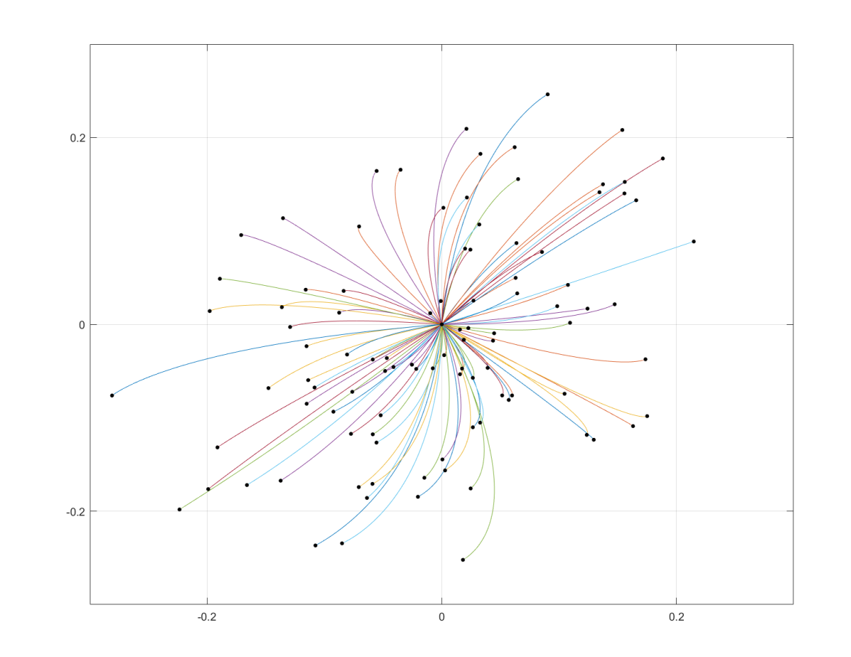
Figure 2: Trajectories of $\dot{z}=\phi^{\theta}(z)$ from the origin for 100 randomly generated realization of the parameter $\theta\in\Theta$. The black dots indicate the resulting equilibria.

In order to guarantee strict contraction in terms of the measurements, we employ the condition of Corollary 4.2. With these measurements $\Phi$ has full row rank and thus $\Theta=\mathcal{Z}(N)$ is compact. For the last assumption, from the fact that $\|J(b)\|_{2}=\sqrt{2}$, we obtain that for any $z,z^{\star}\in\mathbb{R}^{2}$,

$$\vspace{-0.3em}\|b(z)-b(z^{\star})\|_{2,(-N_{22})^{-1/2}}\leqslant\frac{\sqrt{2}}{\sqrt{-\lambda_{\textrm{max}}(N_{22})}}\|z-z^{\star}\|_{2}.$$

This means that we can use Corollary 4.2, which shows that the unknown system is strictly contracting if

$$\vspace{-0.3em}\operatorname{osLip}(\phi^{\operatorname{lse}})<-\frac{\sqrt{2\lambda_{\textup{max}}(N|N_{22})}}{\sqrt{-\lambda_{\textrm{max}}(N_{22})}}\approx-1.78.$$

Using a line of reasoning as in (43) allows us to conclude that this indeed holds. As such, the system $\dot{z}=\phi^{\theta}$ is strictly contracting for all $\theta\in\Theta$. We plot a number of trajectories of the systems corresponding to 4 different realizations of the parameter $\theta$ in Figure 3. It can be seen that each is strictly contracting.

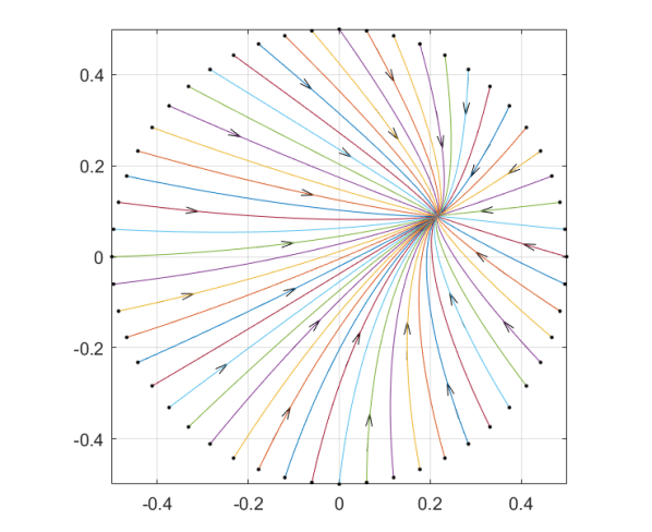
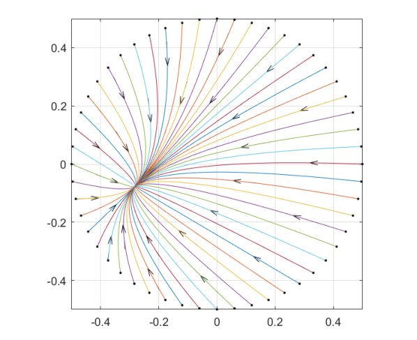
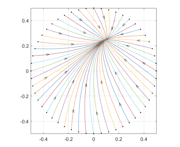
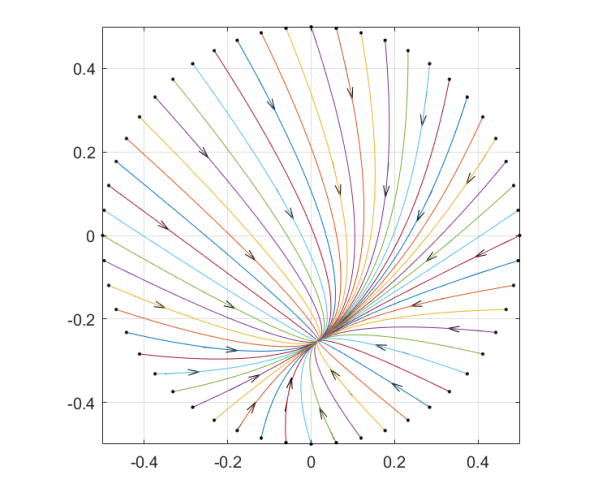
Figure 3: Trajectories of $\dot{z}=\phi^{\theta}(z)$ starting from a number of different initial conditions on the circle with radius $\tfrac{1}{2}$ for four different realizations of $\theta\in\Theta$.

6.2 Suboptimal regulation of unmanned aerial vehicle

This example considers the suboptimal regulation of a fixed-wing unmanned aerial vehicle (UAV). We consider a model of the longitudinal motion for which the relevant equations of motion are derived in e.g., [42, Ch. 2]. For the values of the parameters and the linearization we follow [43], which derives a benchmark model on the basis of 10 different models of real-world UAV’s of different specifications. The derived system is a state-space model

$$\dot{x}(t)=A_{\textrm{cont}}x(t)+B_{\textrm{cont}}u(t),$$

given in [43, Eq. (8)-(10)], with states $x(t)\in\mathbb{R}^{4}$ and inputs $u(t)\in\mathbb{R}$. Here, $x_{1}(t)$ denotes the deviation from the nominal forward velocity, $x_{2}(t)$ the deviation from the nominal angle of attack, $x_{3}(t)$ the pitch angle, and $x_{4}(t)$ the pitch rate. The input $u(t)$ represents the elevator deflection. We use the parameters derived in [43, Eq. (13)-(14)], and thus

$$A_{\textrm{cont}}\!\!=\!\!\scriptsize{\begin{bmatrix}-0.240&0.345&\!\!-0.411&0\\ -1.905&-10.695\!\!&0&\!0.941\\ 0&0&0&1\\ 0.457&-250.513\!\!&0&\!-8.844\end{bmatrix}}\!,B_{\textrm{cont}}\!\!=\!\!\begin{bmatrix}0\\ -0.301\\ 0\\ -98.658\end{bmatrix}\!.\vspace{-0.3em}$$

We consider a discretization of this model with stepsize $\tfrac{1}{20}$, thus arriving at a system of the form (30), where $\hat{A}=I_{4}+\tfrac{1}{20}A_{\textrm{cont}}$ and $\hat{B}=\tfrac{1}{20}B_{\textrm{cont}}$. These matrices are unknown to us, and instead we have access to a single second-long trajectory of measurements of the state $x(t)$ with $x(0)=\tiny{\begin{pmatrix}1&1&1&1\end{pmatrix}^{\top}}$, and fixed input $u(t)=-4$. Thus, $T=20$. Denoting the matrix collecting the noise samples by $W_{s}$, we assume that the noise on the measurements is such that $W_{s}W_{s}^{\top}\leqslant 10^{-4}I_{4}$. These measurements give rise to a set of systems consistent with the data given by $\Sigma=\mathcal{Z}(M)$.

Following Section 4.2, we aim at finding suboptimal values of the norm of an unknown cost function. In this example, we consider a simple cost function $\hat{\phi}:\mathbb{R}^{4}\rightarrow\mathbb{R}^{4}$ of the form $\hat{\phi}(x)=x-\hat{x}$, where $\hat{x}=\tiny{\begin{pmatrix}1&0&0&0\end{pmatrix}^{\top}}$. This situation might arise, for instance, when the UAV is tasked to mirror the orientation and speed of another UAV on the basis of noisy measurements. If the cost function were known, the problem of minimizing $\|\hat{\phi}\|_{2}$ would be to simply regulate $x$ as close to $\hat{x}$ as possible. However, we assume that we only know that $\hat{\phi}$ is affine in $x$, and thus of the form

$$\phi^{\theta}(x):=\theta^{\top}\begin{pmatrix}1\\ x\end{pmatrix},\textrm{ where }\hat{\theta}=\begin{bmatrix}-\hat{x}^{\top}\\ I_{4}\end{bmatrix}.$$

We assume that the measurements available to us are collected concurrently with the collection of the measurements of the unknown system. In line with Section 2, this means that we measure at $z_{i}:=x(i-1)$ for $i=1,\ldots,T=20$. We assume a noise model of the form $WW^{\top}\leqslant I_{4}$, and obtain a set of parameters consistent with the measurements given by $\Theta=\mathcal{Z}(N)$.

We are interested in finding upper bounds for the quantity

$$\vspace{-0.3em}\min_{u}\|\hat{\phi}((I-\hat{A})^{-1}\hat{B}u)\|_{2}.$$

Before applying Theorem 4.8, we need to check its assumptions. First, we employ Lemma 4.4 in order to check whether each $A$ consistent with the measurements is stable. Solving the LMI (31) yields

$$\vspace{-0.3em}\bar{P}\approx\scriptsize{\begin{bmatrix}\vphantom{-}0.0072&0.0015&\vphantom{-}0.0004&-0.0102\\ \vphantom{-}0.0015&0.1665&\vphantom{-}0.1218&\vphantom{-}0.1496\\ \vphantom{-}0.0004&0.1218&\vphantom{-}0.1648&-1.3489\\ -0.0102&0.1496&-1.3489&45.00437\end{bmatrix}}.$$

Next, we employ Lemma 3.16 to obtain a Lipschitz constant. Given that the basis functions are linear, we can easily minimize $L$ over (25) to obtain $L=2.0171$. Thus, $L$ is a Lipschitz constant for $\phi^{\theta}$ for all $\theta\in\mathcal{Z}(N)$.

Therefore, the required pieces are in place, and we can employ Theorem 4.8 to show that

$$\min_{u}\|\hat{\phi}((I-\hat{A})^{-1}\hat{B}u)\|_{2}\leqslant 2.3347.$$ (44)

This value in attained for the input $u^{\star}=0.2321$ and the minimizer in the state is $x=\scriptsize\begin{pmatrix}0.809&0.054&-0.355&-0.006\end{pmatrix}^{\!\top}$.

Figure 4 shows the results of applying this input to different realizations of the system matrices compatible with the measurements. We make the following observations. First, one can see that each of the systems converges to a fixed point, and each of these fixed points are within a distance $\varepsilon^{-}(x)=0.4491$ of $x$. Second, for certain systems the transients, especially in states $x_{1}$ and $x_{2}$, converge quite slowly. This holds because the true system is marginally stable and the same holds for elements of set $\mathcal{Z}(M)$ (to be precise, the upper bound of Theorem 4.9 can only be shown to hold for $0.999<\lambda<1$).

Corresponding to these trajectories, Figure 5 shows the resulting values of $\|\phi^{\theta}(x_{k})\|_{2}$, for both the true value and for different realizations of $\theta\in\mathcal{Z}(N)$. The plot reveals shows that, with the true parameter $\hat{\theta}$, the values at the fixed points are well below the bound (44). In fact, resolving the problem with known $\hat{\phi}$ yields $u^{\star}=0.1820$ and an upper bound of $0.7963$. Indeed, as the left plot shows, the unknown nature of $\hat{\phi}$ has a large effect and therefore has to be taken into account when providing formal guarantees.

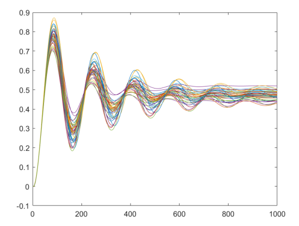
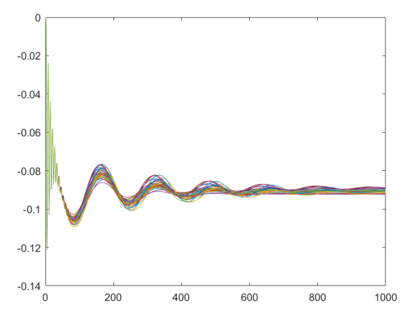
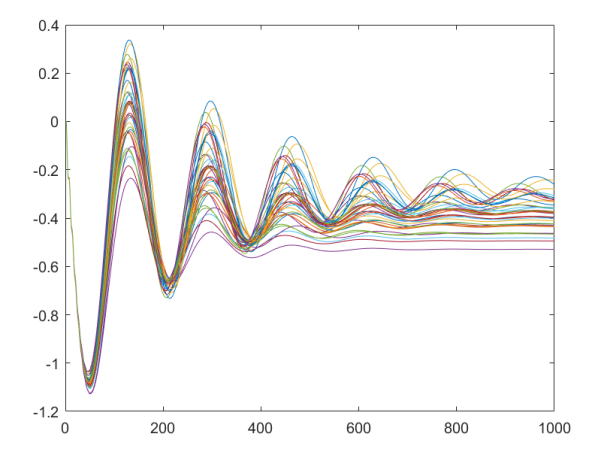
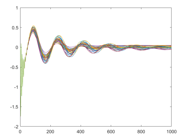
Figure 4: State trajectory corresponding to the found input $u^{\star}=0.2321$ for 40 different realizations of the matrices $(A,B)$ consistent with the measurements.

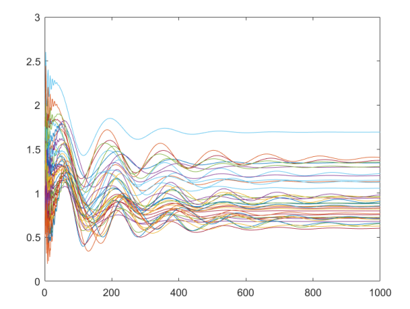
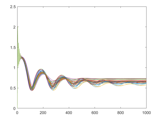
Figure 5: Values of $\|\phi^{\theta}(x_{k})\|_{2}$ for the state trajectories of Figure 4. On the left, we pick for each system a different realization of $\theta\in\mathcal{Z}(N)$. On the right, we use the true value of $\hat{\theta}$.

7 Conclusions

We have developed a set-valued regression approach to data-based optimization of an unknown vector-valued function. Taking a worst-case perspective, we have provided a range of guarantees in terms of measurements on the minimization of least conservative upper bounds of both the norm and any linear combination of the components of the unknown function. Our analysis has yielded closed-form expressions for the proposed upper bounds, conditions to ensure their convexity (as an enabler for the use of gradient-based methods for their optimization), and Lipschitzness characterizations to facilitate simplifications based on interpolation. We have illustrated the applicability of the proposed cautious optimization approach in systems and control scenarios with unknown dynamics: first, by providing conditions on the data which guarantee that the dynamics is strongly contracting and, second, by providing conditions under which we can regulate an unknown system to a point with a guaranteed maximal value of an unknown cost function. Finally, we have considered online scenarios, where one repeatedly combines the optimization of the unknown function with the collection of additional data. Under mild assumptions, we show that repeated measurements lead to a strictly shrinking set of compatible parameters and we build on this result to design an online procedure that provides sequential upper bounds which converge to a true optimizer.

Future work will investigate conditions to ensure other regularity properties of the unknown function and its least conservative upper bounds, the impact of the choice of basis functions on the guarantees and computational efficiency of the proposed cautious optimization methods (particularly, the use of polynomial bases coupled with sum-of-squares optimization techniques), and the application of the results to the certification of Lyapunov stability and controller design for nonlinear systems.

References

• [1] J. Eising and J. Cortés, “Set-valued regression and cautious suboptimization: from noisy data to optimality,” in IEEE Conf. on Decision and Control, Singapore, 2023, submitted.
• [2] A. Ben-Tal, L. E. Ghaoui, and A. Nemirovski, Robust Optimization, ser. Applied Mathematics Series.   Princeton, NJ: Princeton University Press, 2009.
• [3] D. Bertsimas, D. B. Brown, and C. Caramanis, “Theory and applications of robust optimization,” SIAM Review, vol. 53, no. 3, pp. 464–501, 2011.
• [4] C. E. Rasmussen and C. K. I. Williams, Gaussian Processes for Machine Learning.   The MIT Press, Nov. 2005.
• [5] M. Milanese and A. Vicino, “Optimal estimation theory for dynamic systems with set membership uncertainty: An overview,” Automatica, vol. 27, no. 6, pp. 997–1009, 1991.
• [6] M. Milanese and C. Novara, “Set membership estimation of nonlinear regressions,” in IFAC World Congress, vol. 35, no. 1, Barcelona, Spain, 2002, pp. 7–12.
• [7] J. Calliess, S. J. Roberts, C. E. Rasmussen, and J. Maciejowski, “Lazily adapted constant kinky inference for nonparametric regression and model-reference adaptive control,” Automatica, vol. 122, p. 109216, 2020.
• [8] G. Cybenko, “Dynamic load balancing for distributed memory multiprocessors,” Journal of Parallel and Distributed Computing, vol. 7, no. 2, pp. 279–301, 1989.
• [9] P. Tabuada and B. Gharesifard, “Universal approximation power of deep residual neural networks through the lens of control,” IEEE Transactions on Automatic Control, vol. 68, no. 5, pp. 2715–2728, 2023.
• [10] M. Budišić, R. Mohr, and I. Mezić, “Applied Koopmanism,” Chaos, vol. 22, no. 4, p. 047510, 2012.
• [11] M. Korda and I. Mezic, “Optimal construction of Koopman eigenfunctions for prediction and control,” IEEE Transactions on Automatic Control, vol. 65, no. 12, pp. 5114–5129, 2020.
• [12] M. Haseli and J. Cortés, “Generalizing dynamic mode decomposition: balancing accuracy and expressiveness in Koopman approximations,” Automatica, vol. 153, p. 111001, 2023.
• [13] T. Hastie, R. Tibshirani, and J. Friedman, The Elements of Statistical Learning: Data Mining, Inference, and Prediction, 2nd ed., ser. Springer Series in Statistics.   New York: Springer, 2013.
• [14] R. Tibshirani, “Regression shrinkage and selection via the Lasso,” Journal of the Royal Statistical Society. Series B, vol. 58, no. 1, pp. 267–288, 1996.
• [15] S. L. Brunton, J. L. Proctor, and J. N. Kutz, “Discovering governing equations from data by sparse identification of nonlinear dynamical systems,” Proceedings of the National Academy of Sciences, vol. 113, no. 15, pp. 3932–3937, 2016.
• [16] P. J. Schmid, “Dynamic mode decomposition of numerical and experimental data,” Journal of Fluid Mechanics, vol. 656, pp. 5–28, 2010.
• [17] ——, “Dynamic mode decomposition and its variants,” Annual Review of Fluid Mechanics, vol. 54, no. 1, pp. 225–254, 2022.
• [18] J. N. Kutz, S. L. Brunton, B. W. Brunton, and J. L. Proctor, Dynamic Mode Decomposition: Data-Driven Modeling of Complex Systems, ser. Other Titles in Applied Mathematics.   Philadelphia, PA: SIAM, 2016, vol. 149.
• [19] M. R. Jovanović, P. J. Schmid, and J. W. Nichols, “Sparsity-promoting dynamic mode decomposition,” Physics of Fluids, vol. 26, no. 2, p. 024103, 2014.
• [20] J. C. Willems, P. Rapisarda, I. Markovsky, and B. L. M. De Moor, “A note on persistency of excitation,” Systems & Control Letters, vol. 54, no. 4, pp. 325–329, 2005.
• [21] H. J. van Waarde, J. Eising, H. L. Trentelman, and M. K. Camlibel, “Data informativity: a new perspective on data-driven analysis and control,” IEEE Transactions on Automatic Control, vol. 65, no. 11, pp. 4753–4768, 2020.
• [22] I. Markovsky, “Data-driven simulation of generalized bilinear systems via linear time-invariant embedding,” IEEE Transactions on Automatic Control, vol. 68, no. 2, pp. 1101–1106, 2022.
• [23] M. Guo, C. D. Persis, and P. Tesi, “Data-driven stabilization of nonlinear polynomial systems with noisy data,” IEEE Transactions on Automatic Control, vol. 67, no. 8, pp. 4210–4217, 2021.
• [24] C. De Persis, M. Rotulo, and P. Tesi, “Learning controllers from data via approximate nonlinearity cancellation,” IEEE Transactions on Automatic Control, 2023, to appear.
• [25] V. G. Lopez and M. A. Müller, “On a continuous-time version of Willems’ lemma,” arXiv preprint arxiv:2203.03702, 2022.
• [26] P. Rapisarda, M. K. Camlibel, and H. van Waarde, “A persistency of excitation condition for continuous-time systems,” IEEE Control Systems Letters, vol. 7, pp. 589–594, 2022.
• [27] J. Eising and J. Cortés, “When sampling works in data-driven control: informativity for stabilization in continuous time,” IEEE Transactions on Automatic Control, 2023, submitted. Available at https://arxiv.org/abs/2301.10873.
• [28] W. Lohmiller and J.-J. E. Slotine, “On contraction analysis for non-linear systems,” Automatica, vol. 34, no. 6, pp. 683–696, 1998.
• [29] F. Bullo, Contraction Theory for Dynamical Systems, 1.1 ed.   Kindle Direct Publishing, 2023.
• [30] F. Dörfler, P. Tesi, and C. De Persis, “On the certainty-equivalence approach to direct data-driven LQR design,” IEEE Transactions on Automatic Control, 2023, to appear.
• [31] G. Bianchin, M. Vaquero, J. Cortés, and E. Dall’Anese, “Online stochastic optimization of unknown linear dynamical systems: data-driven controller synthesis and analysis,” IEEE Transactions on Automatic Control, 2021, submitted.
• [32] A. Hauswirth, S. Bolognani, G. Hug, and F. Dörfler, “Optimization algorithms as robust feedback controllers,” arXiv preprint arXiv:2103.11329, 2021.
• [33] L. Cothren, G. Bianchin, and E. Dall’Anese, “Data-enabled gradient flow as feedback controller: Regulation of linear dynamical systems to minimizers of unknown functions,” in Conference on Learning for Dynamics and Control, ser. Proceedings of Machine Learning Research, vol. 168.   PMLR, 2022, pp. 234–247.
• [34] M. Krstić and H.-H. Wang, “Stability of extremum seeking feedback for general nonlinear dynamic systems,” Automatica, vol. 36, no. 4, pp. 595–601, 2000.
• [35] K. B. Ariyur and M. Krstić, Real-Time Optimization by Extremum-Seeking Control.   New York: Wiley, 2003.
• [36] A. Teel and D. Popovic, “Solving smooth and nonsmooth multivariable extremum seeking problems by the methods of nonlinear programming,” in American Control Conference, Arlington, VA, 2001, pp. 2394–2399.
• [37] H. J. van Waarde, M. K. Camlibel, J. Eising, and H. L. Trentelman, “Quadratic matrix inequalities with applications to data-based control,” arXiv preprint arXiv:2203.12959, 2022.
• [38] I. Pólik and T. Terlaky, “A survey of the S-Lemma,” SIAM Review, vol. 49, no. 3, pp. 371–418, 2007.
• [39] S. Boyd and L. Vandenberghe, Convex Optimization.   Cambridge, UK: Cambridge University Press, 2009.
• [40] A. Davydov, S. Jafarpour, and F. Bullo, “Non-Euclidean contraction theory for robust nonlinear stability,” IEEE Transactions on Automatic Control, vol. 67, no. 12, pp. 6667–6681, 2022.
• [41] H. J. van Waarde, M. K. Camlibel, and H. L. Trentelman, “Data-driven analysis and design beyond common Lyapunov functions,” in IEEE Conf. on Decision and Control, 2022, pp. 2783–2788.
• [42] J. H. Blakelock, Automatic Control of Aircraft and Missiles.   John Wiley & Sons, 1991.
• [43] E. Bertran, P. Tercero, and A. Sànchez-Cerdà, “UAV generalized longitudinal model for autopilot controller designs,” Aircraft Engineering and Aerospace Technology, vol. 94, no. 3, pp. 380–391, 2022.