Volumetric Wireframe Parsing from Neural Attraction Fields

Abstract

The primal sketch is a fundamental representation in Marr’s vision theory, which allows for parsimonious image-level processing from 2D to 2.5D perception. This paper takes a further step by computing 3D primal sketch of wireframes from a set of images with known camera poses, in which we take the 2D wireframes in multi-view images as the basis to compute 3D wireframes in a volumetric rendering formulation. In our method, we first propose a NEural Attraction (NEAT) Fields that parameterizes the 3D line segments with coordinate Multi-Layer Perceptrons (MLPs), enabling us to learn the 3D line segments from 2D observation without incurring any explicit feature correspondences across views. We then present a novel Global Junction Perceiving (GJP) module to perceive meaningful 3D junctions from the NEAT Fields of 3D line segments by optimizing a randomly initialized high-dimensional latent array and a lightweight decoding MLP. Benefitting from our explicit modeling of 3D junctions, we finally compute the primal sketch of 3D wireframes by attracting the queried 3D line segments to the 3D junctions, significantly simplifying the computation paradigm of 3D wireframe parsing. In experiments, we evaluate our approach on the DTU and BlendedMVS datasets with promising performance obtained. As far as we know, our method is the first approach to achieve high-fidelity 3D wireframe parsing without requiring explicit matching.

1 Introduction

This paper studies the problem of multi-view 3D reconstruction from the perspective of primal sketch [22], aiming at explicitly computing a parsimonious and accurate representation of 3D scenes from posed multi-view images. Marr’s vision theory [22] has long laid out a computational paradigm in which 2D and 2.5D primal sketches are key representations for image and view-dependent scene geometry in perception and understanding, motivating us to move forward to computing primal sketches of 3D scenes.

In recent years, wireframes [51] has been proposed as a parsimonious yet expressive representation scheme focusing on the boundary-oriented primal sketch of 2D images. By unifying edge maps, line segments, and junctions all in one task of wireframe parsing, we have witnessed their great success in the geometric characterization of images for man-made environments and indoor images in wireframes. A wireframe consists of junctions as the graph vertices and line segments as the graph edges [50, 44, 28, 45, 27, 42, 43]. However, the current state of the art in wireframe-based scene characterization mainly focuses on either the image-level structural perception or the single-view 3D perception [51].

For the 3D wireframe parsing from multi-view images, it was studied as a line-based multi-view 3D reconstruction [14] problem in which the key is to build line correspondences across views. Because of the view-dependent occlusion of underlying 3D line segments in the detected 2D line segments, such a correspondence-based pipeline often does not work well on top of the holistic line segments from the wireframe graphs by the deep wireframe parsers [45]. As shown in the left of Fig. Volumetric Wireframe Parsing from Neural Attraction Fields, due to the difficulty of line segment matching between 2D wireframes, many meaningful 2D line segments are ignored by Line3D++ [14] to yield an incomplete 3D wireframe model from 2D detection results. Instead, the correspondence-based pipelines are built on the small line fragments by the traditional LSD approach [36], which leads to fragmented and noisy 3D wireframe parsing results. More importantly, 3D junctions (i.e. vertices of a 3D wireframe graph) are not explicitly computed in, and seem not practically feasible to be reliably tackled by, such a correspondence-based pipeline.

Most recently, we have witnessed the great success in neural implicit rendering for multi-view 3D reconstruction [24, 2, 3, 48, 47, 38, 25]. It highlights the exciting fact that the scene geometry can be optimized well via coordinate MLPs without entailing explicit cross-view correspondences. Accordingly, we raise a question:

Could we accomplish 3D wireframe parsing from multi-view input images without incurring explicit 2D wireframe correspondences?

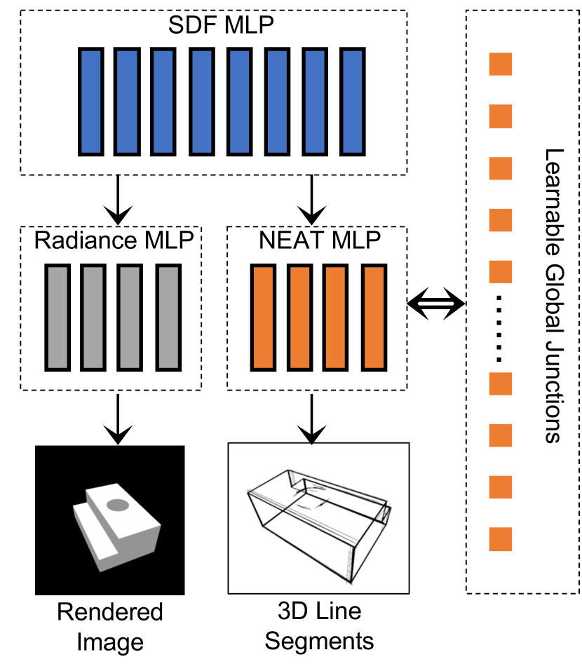
(a). NEAT Field Learning

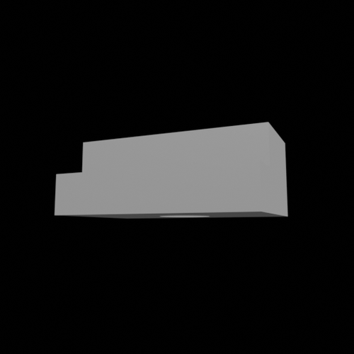
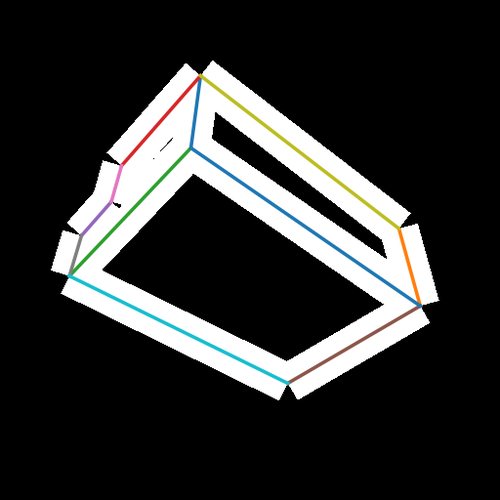
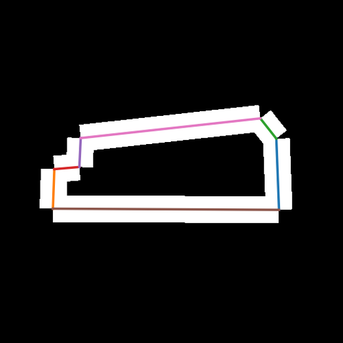
(b). Input Images and 2D Wireframes

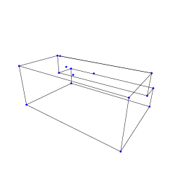
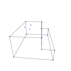
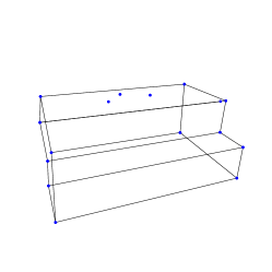
(c). 3D Wireframe Model by NEAT Field

Figure 2: The proposed NEAT field learning framework for volumetric wireframe parsing. For clarity, we use multi-view images of a synthetic 3D object in the ABC dataset [18] to illustrate the proposed method. (a) Our NEAT field is built on the Signed Distance Function (SDF) based density volume representation [47]. The NEAT field is used to render 3D line segments, and “interacts” with a Global 3D Junction Perceiving (GJP) module. (b) shows the two examples of the input images and the regional representation (white regions) of 2D wireframes (line segments in colors) computed by an off-the-shelf 2D wireframe parser [45]. We only query rays that intersect with the 2D attraction regions (white) during volume rendering. (c) 3D wireframe examples computed by our method. See text for details.

The answer is Yes! We firmly address it by proposing a novel approach, the NEural ATtraction (NEAT) field for 3D wireframe parsing (Fig. 2 (a)) in two-fold as follows.

The meaningfulness of rendering 3D line segments by querying 2D wireframe guided rays in the NEAT field. We use as inputs multi-view 2D wireframes computed by a state-of-the-art self-supervised 2D wireframe parser [45], together with raw input multi-view images (Fig. 2 (b)). To eliminate the need of building cross-view correspondences between the 2D wireframes, our NEAT-field directly renders 3D line segments by querying view-dependent rays that intersect with 2D wireframes (more specifically, the 2D attraction regions associated with 2D wireframes proposed in [44, 45]) under the volume rendering integral formulation [24]. We verified that by only querying the 2D wireframe guided rays (that are sparse compared with the counterparts in the vanilla volume rendering) the implicit scene geometry can still be optimized sufficiently well. The restulting 3D line segment cloud computed by our NEAT field is promising and meaningful, but noisy (Fig. Volumetric Wireframe Parsing from Neural Attraction Fields). 3D junctions are entailed to “clean up” the noisy rendered 3D line segments.

⬇ def __init__(self, num_junctions, dim=256, **kwargs): ... self.latents = nn.Parameters(num_junctions, dim,...) self.junction_mlp = nn.Sequential(nn.Linear(dim,dim),nn.ReLU(), nn.Linear(dim,dim),nn.ReLU(), nn.Linear(dim,3)) ... def compute_global_junctions(self): return self.junction_mlp(self.latents)

The surprising effectiveness of directly perceiving global 3D junctions in the NEAT field. It is tempting to render 3D junctions by querying rays passing through 2D junctions in the 2D wireframe, which does not work due to the intrinsic geometry ambiguity. Counterintuitively, we present a novel mechanism, the Global Junction Perceiving (GJP) to learn the 3D junctions across viewpoints, which is best illustrated by the code snippet shown above.

It is counterintuitive because the latent queries (as model parameters) are directly transformed into 3D junctions via an MLP. Both the latent queries and the junction MLP are learned on the fly, and yet they can coverge to predict the 3D junctions reliably (Fig. Volumetric Wireframe Parsing from Neural Attraction Fields). We exploit the synergies between 3D junctions and end-points of 3D line segments in a 3D wireframe in learning. Although noisy, the rendered 3D line segments provide sufficient “local evidence” in the 3D space for “regularizing” the learning of GJP. We utilize the Hungarian matching in learning to match the “local evidence” from volume rendering and the GJP outputs. After the GJP converges, the perceived global 3D junctions are stable and in turn provide binging forces to “clean up” the noisy rendered 3D line segments. Together, they form the reconstructed 3D wireframe. This surprising effectiveness of GJP reinforces the exciting fact that the implicit scene geometry that can be optimized well via coordinate MLPs in the volumetric rendering formulation can be concurrently optimized for volumetric 3D wireframe parsing with our NEAT field, but without entailing explicit cross-view correspondences.

We test our proposed NEAT field on the DTU [1] and BlendedMVS [46] datasets and promising results are obtained. In sum, this paper makes three main contributions to the field of volumen rendering and 3D wireframe parsing:

• To the best of our knowledge, we are the first to achieve the multi-view 3D wireframe reconstruction. Without leveraging any heuristic correspondence search across viewpoints, we exaggerate the powerful capability of coordinate MLPs (implicit neural networks) for implicit feature correspondences.

• We present a novel NEAT field to learn sparse structures (3D line segments and 3D junctions) from the dense volumetric representation of rendering. On the one hand, we demonstrated that the regional association between rays queried in rendering and 2D line segments is a powerful tool to learn the sparse representation of 3D line segments from the dense volume. On the other hand, our novel design of directly perceiving the global 3D junctions from the randomly initialized latent queries provides a promising way to represent the scene geometry in a parsimonous and unified way.

• In experiments, we show that our NEAT field significantly pushes the boundary of 3D wireframe reconstruction to simultaneously handle both straight-line dominated scenes and curve-based (or polygonal line segment dominated) scenes, paving a way towards learning 3D primal sketch. Our proposed GJP opens a door to characterize the scene geometry from 2D supervision in structured point-level 3D representations.

2 Related Work

Structured 3D Reconstruction with Lines.

Because of the inherent structural regularities for scene representation conveyed by line structures [22, 31, 21, 12, 34], there has been a vast body of literature on line-based multiview 3D reconstruction tasks including line-based SfM [30, 5], SLAM [29, 39], and multi-view stereo [14] based on the theory of multi-view geometry [13]. Due to the challenging difficulties of line segment detection and matching in 2D images, most of those studies expected the 2D line segments detected from input images to be redundant and small-length to maximize the possibility of line segment matching. As for the estimation of scene geometry and camera poses, the keypoint correspondences (even including the 3D point clouds) are usually required. For example in Line3D++ [14], given the known camera poses by keypoint-based SfM systems [32, 33, 35, 40], it is still challenging though to establish reliable correspondences for the pursuit of structural regularity for 3D line reconstruction. For our goal of wireframe reconstruction, because 2D wireframe parsers aim at producing parsimonious representations with a small number of 2D junctions and long-length line segments, those correspondence-based solutions pose a challenging scenario for cross-view wireframe matching, thus leading to inferior results than the ones using redundant and small-length 2D line segments detected by LSD [36]. To this end, we present a correspondence-free formulation based on coordinate MLPs, which provides a novel perspective to accomplish the goal of 3D wireframe reconstruction from the parsed 2D wireframes.

Neural Rendering for Geometry Primitives.

In recent years, the emergence of neural implicit representations [24, 2, 48, 23] have greatly renown the 3D vision community. By using coordinate MLPs to implicitly learn the scene geometry from multi-view inputs without knowing either the cross-view correspondences or the 3D priors, it has largely facilitated many 3D vision tasks including novel view synthesis, multi-view stereo, surface reconstruction, etc. Some recent studies further exploited the neural implicit representations by (explicitly and implicitly) taking the geometric primitives such as 2D segmentation masks into account to lift the 2D detection results into 3D space for scene understanding and interpretation [10, 20, 37, 41]. Most recently, nerf2nerf [11] exploited a geometric 3D representation, surface fields as a drop-in replacement for point clouds and polygonal meshes, and takes the keypoint correspondences to register two NeRF MLPs. Our study can be categorized as the exploration of geometric primitives in neural implicit representation, but we focus on computing a parsimonious representation by using the most fundamental geometric primitives, the junction (points) and line segments, to provide a compact and explicit representation from coordinate MLPs.

3 Problem Statement

In this section, we first define the problem, and give a high-level formulation, of lifting dense volume rendering of neural implicit surfaces to parsimonious 3D wireframe parsing (Sec. 3.1). Our formulation takes the multi-view images and the corresponding 2D wireframes detected by an off-the-shelf wireframe parser, HAWP [45] (Sec. 3.2). Building on the top of the volumetric surface rendering [47] along the queried rays emanating from the camera location $c$ with the view dicrection $v$

$$\hat{I}(c,v)=\int_{0}^{\infty}T(t)\cdot\sigma(x_{t})\cdot\mathbf{r}(x_{t},v,\mathbf{n}(x_{t}),z(x_{t}))dt,$$ (1)

with the transmittance $T(t)=\exp-\int_{0}^{t}\sigma\left(x(s)\right)ds$, we get rid of explicit feature correspondences for 3D wireframe parsing in Sec. 4.

3.1 The Problem of 3D Wireframe Parsing

Denoted by $x(t)=c+t\cdot v$ for a ray $x$ emanating from a camera center $c\in\mathbb{R}^{3}$ along the unit direction $v$, we formulate the problem of 3D wireframe parsing based on VolSDF, which learns the signed distance $d(x_{t})$ and the surface feature $z(x_{t})$ at the queried 3D location $x_{t}$ and then compute the radiance field $\mathbf{r}(x_{t},v,\mathbf{n}(x_{t}),z(x_{t})$, where $\mathbf{n}(x_{t})=\nabla_{x}d(x_{t})$ is the surface normal determined by the SDF. In practical computation, the coordinate MLPs are used for the learning of SDF and radiance field.

Intuitively, our proposed volumetric wireframe parsing is to compute the line drawing of those implicit surfaces using the 3D wireframe representation. A 3D wireframe of a scene is represented by a graph $\mathcal{G}=(\mathcal{J},\mathcal{L})$, where $\mathcal{J}$ is the vertex set consisting of 3D junctions, $J_{i}\in\mathbb{R}^{3}$, and $\mathcal{L}$ is the edge set consisting of 3D line segments. A 3D line segment, $L_{i,j}$, connects two 3D junctions (i.e., end-points), $J_{i}$ and $J_{j}$.

Our proposed volumetric wireframe parsing is built on top of the VolSDF and consists of three components:

• 3D Line Segment Rendering:

  $$\small(x_{t},v)\xrightarrow[]{}(x_{t},x_{t})+(\Delta x_{t}^{1},\Delta x_{t}^{2})=L(x_{t},v,\mathbf{n},z),$$ (2)

  where $(\Delta x_{t}^{1},\Delta x_{t}^{2})$ are the displacement/offset vectors of the 3D line segment at the 3D query point $x_{t}$. We will address the problem of which rays will be sampled in order to ensure the learning of both Eqn. 1 and Eqn. 2 based on the 2D wireframe observations, and compute the 3D line segment rendering integral to generate 3D line segment proposals.

• Global 3D Junction Percieving: Our 3D line segment rendering inherits the dense representation as the density field and the radiance field. To achieve parsimonious wireframes, we propose a novel query-based design to holistically perceive a predefined sparse set of $N$ 3D junctions by

  $$Q_{N\times C}\xrightarrow[]{\text{MLP}}J_{N\times 3},$$ (3)

  where $Q_{N\times C}$ are $C$-dim latent queries (randomly initialized in learning). Surprisingly, as we shall show in experiments, the underlying 3D scene geometry induced synergies (Sec. 4.2) between $J_{N\times 3}$ and the above 3D line segment rendering integral enable us to learn a very meaningful global 3D junction perceiver. To put it in another way, the 3D junction perceiver is learned to geometrically attract the dense 3D line segment rendering integral to a sparse set of junctions in the 3D space. Due to this attraction nature, we dub the proposed representation scheme short in NEAT.

• 3D Wireframe Reconstruction: With the 3D line segment proposals (Eqn. 2) and the 3D junction proposals (Eqn. 3), we extend the 2D wireframe parsing method proposed in [45] for 3D wireframe reconstruction as the final step in Sec. 4.3.

3.2 2D Wireframes and the Ray Sampling

In this section, we elaborate on the inputs that are needed in the proposed 3D line segment rendering (Eqn. 2) and on what rays to be sampled in learning to satisfy both Eqn. 1 and Eqn. 2. We leverage the self-supervised HAWPv3 [45] model (trained on a subset of ImageNet data)  as the wireframe parser due to their outperforming OOD performance throughout our experiments.

For simplicity, consider an image $I$ in a given set of multi-view images in learning, we denote by $L^{\rm 2D}=\{\ddot{l}_{i}=(\mathbf{x}_{i}^{1},\mathbf{x}_{i}^{2})\}_{i=1}^{M}$ the set of 2D line segments in the parsed 2D wireframe for $I$. In terms of ray sampling, one straightforward method is to only sample rays that intersect with a 2D line segment in $L$. Unfortunately, this will become too sparse to optimize the coordinate MLPs,which in turn impacts the learning of the 3D line segments (Eqn. 2). To address this issue, we exploit the basic idea of lifting a 2D line segment to its attraction region proposed in HAWP [45] to densify the sparse geometry with the non-edge pixels. The attraction region of a line segment $\ddot{l}_{i}$, denoted by $a(\ddot{l}_{i})$, consists of pixels whose distances to the line segment are smaller than a predefined threshold (e.g., 10 pixels). We will consider the set of all rays that intersect with any pixels in all the 2D attraction regions in ray sampling in learning.

With this relaxation, we verified that the ray sampling enables the high-fidelity rendering of images based on Eqn. 1, as shown in Fig. 2 and our supplementary materials. We also assign 2D line segments $\ddot{l}_{i}$ as the ground-truth 2D observation for 3D line segments rendered from any rays that intersect with a pixel in the attraction region $a(\ddot{l}_{i})$ based on Eqn. 2.

4 The Proposed NEAT Fields

In this section, we present details of the three components in our volumetric wireframe parsing.

4.1 3D Line Segment Rendering

Similar to the computation of the expected color (Eqn. 1), with the 3D line segment rendering (Eqn. 2), we compute the two displacement vectors of the expected 3D line segment along a ray $x(t)$ by,

$$\ddot{L}(c,v)=\int_{0}^{\infty}T(t)\cdot\sigma(x_{t})\cdot L(x_{t},v,\mathbf{n}(x_{t}),z(x_{t}))dt,$$ (4)

where $\ddot{L}(c,v)\in R^{2\times 3}$. We follow the point sampling algorithm proposed in VolSDF [47] in approximating the integral empirically.

Denote by $\Pi(\ddot{L}(c,v))$ the projected 2D line segment to the image plane of the camera emitting the ray $x(t)$, and by $\ddot{l}(c,v)$ the observed 2D line segment (computed by the HAWPv3) that intersects with the ray $x(t)$. The loss between $\Pi(\ddot{L}(c,v))$ and $\ddot{l}$ is defined by the minimum $l_{1}$ distance between the projected and observed 2D line segments over the permutation of the order of the two end-points,

$$\mathcal{L}_{\rm neat}(\ddot{L},\ddot{l})=\min_{\chi}\|\Pi(\ddot{L})-\chi(\ddot{l})\|_{1},$$ (5)

where $\chi$ represents the two permutations of swapping the two end points of a 2D line segment.

4.2 Global 3D Junction Perceiving

Due to the many-to-one mapping between the associated rays and a 2D line segment observation in 3D line segment rendering, we obtain many redundant 3D line segment proposals. To “clean up” them, global scene geometry is entailed. We present a counter-intuitive yet surprisingly effective query-based learning method for 3D junction perceiving (Eqn. 3), similar in spirit to the DETR [4] and the Perceivers [16, 15], but without using their sophisticated designs of self-attention and cross-attention. We use a plain MLP with randomly initialized queries as the inputs (Eqn. 3).

Since we do not have any well-defined ground-truth observations in learning 3D junctions, we exploit the end-points of the redundant rendered 3D line segments (Sec. 4.1) as the noisy labels. Denote by $\mathbf{J}_{M\times 3}$ the set of end-points from all the current rendered 3D line segments (Eqn. 4). To deal with the noisy labels, our 3D junction perceiving consists of three steps:

• Filtering $\mathbf{J}_{M\times 3}$ to remove the end-points that do not have observed 2D junction support after projection, that is their projections’ minimum distances to the set of observed 2D junctions are larger than a predefined threshold (e.g., 10 pixels). Denote by $\mathbf{J}_{M^{\prime}\times 3}$ the set of end-points after filtering.

• Clustering $\mathbf{J}_{M^{\prime}\times 3}$ to eliminate the redundance caused by the many-to-one relationships between rays and 2D line segement observation. We utilize the DBScan method [9] in clustering. Denote by $\mathbf{J}_{m\times 3}$ the set of end-points after clustering ($m<M$).

• Bi-pariate set-to-set matching between the perceived junctions $J_{N\times 3}$ (Eqn. 3) and the filtered and clustered noisy labels $\mathbf{J}_{m\times 3}$. We use the Hungarian algorithm [19]. The pair-wise matching cost is computed by the $\ell_{2}$ norm between 3D points. Denote by $\mathcal{J}=\{(J_{k\times 3},\mathbf{J}_{k\times 3})_{k=1}^{K}\}$ the set of matched junctions, where $K=\min(N,m)$.

Based on the bipartite matching results, the loss between a perceived junction $J_{k}$ and its assigned “ground-truth” $\mathbf{J}_{k}$ is defined by,

$$\mathcal{L}_{jc}(J_{k},\mathbf{J}_{k})=\left\|J_{k}-\mathbf{J}_{k}\right\|_{1}+\lambda\cdot\left\|\Pi(J_{k})-\Pi(\mathbf{J}_{k})\right\|_{1},$$ (6)

where $\Pi()$ is the 3D-to-2D projection, and $\lambda$ the trade-off parameters (e.g. 0.01 in our experiments).

4.3 3D Wireframe Reconstruction

After optimization, the $N$ global junctions $\{\mathcal{J}_{k}\}$ are saved as the model parameters and the dense 3D line segments (i.e., NEAT lines) are accessed by querying all the foreground rays across viewpoints from NEAT fields. In this stage, we use very “thin” attraction regions with the attraction threshold being 1 pixel for the computing of NEAT lines. Then, three key steps are used for the final 3D wireframe reconstruction.

3D Junction Refinement.

Thanks to the properties of SDF, the learned global junctions by the feed-forward layer can be further refined per the SDF values and their normals by

$$\mathcal{J}_{k}^{\rm refined}=\mathcal{J}_{k}-d(\mathcal{J}_{k})\nabla d(\mathcal{J}_{k}).$$ (7)

For the junctions that have larger SDF values (i.e., $|d(\mathcal{J}_{k})|>0.05$), we directly remove them as they are not reliable to yield the final 3D wireframe model.

The Attraction Scheme.

Similar to what HAWP done for 2D wireframe parsing [45], we use the junctions $\mathcal{J}^{\rm refined}$ as the final endpoints of the 3D line segments to attract the nearest 3D NEAT lines. Then, a wireframe model with $\{\mathcal{J}_{\rm refined}\}$ as the vertices, and the attracted indices $\{(k_{i}^{1},k_{i}^{2})\}$ can be directly transformed to the endpoint representation of the $i$-th 3D line segments. Benefitting from the global junctions, the Attraction Scheme could directly deduplicate the noisy and duplicated 3D line segments across multiview images without considering the cross-view correspondences beforehand. However, such a putative wireframe model would lead up to some unreasonable 3D line segments, which can be filtered by visibility checking to fit the 2D observations.

Visibility Checking.

We use the camera projection matrices to check the visibility of each 3D line segment by comparing their reprojected distance with the 2D detection results. Here, we use a relaxed threshold for each view but require the line segments in the final model should be visible on at least 5 views. See more details in the supplementary.

4.4 Implementation Details

Our NEAT approach is implemented on PyTorch [26] and the source code will be publicly available for reproducible research purposes. For the requirement of 2D wireframes, we use the self-supervised HAWPv3 model [45] trained on the ImageNet data as the detector and keep all the default configurations in our experiments.

The Specification of MLPs.

To keep the simplicity of designs simple enough, the specification of MLPs for the SDF and the radiance field is the same as VolSDF [47]. For the proposed NEAT field, we use a $4$-layer MLP to render the 3D line segments from the queried rays.

Total Loss Function.

For the optimization, we jointly learn the coordinate MLPs and the Global Junction Perceiving module from scratch by scenes. The total loss function $\mathcal{L}_{\text{total}}$ is a weighted-sum by all the mentioned loss items in

$$\mathcal{L}_{\text{total}}=\mathcal{L}_{\rm rend}+\lambda_{n}\mathcal{L}_{\rm neat}+\lambda_{e}\mathcal{L}_{\rm eikonal}+\lambda_{j}\mathcal{L}_{jc},$$ (8)

where the rendering loss $\mathcal{L}_{\rm rend}$ and Eikonal loss $\mathcal{L}_{\rm eikonal}$ are the same with VolSDF [47]. The weights $\lambda_{n},\lambda{e}$ and $\lambda_{j}$ are all set to $0.01$.

Optimizer and Hyperparameters.

We use ADAM [17] as our optimizer. In each iteration, the batch size of the ray sampling is $1024$, and the initial learning rate is set to $5\times 10^{4}$. The exponential learning rate schedule is used, which decays the learning rate in each step by a decay rate of 0.1.

5 Experiments

In experiments, we mainly testify our NEAT on two datasets (i.e., the DTU dataset [1] and the BMVS dataset [46]) for real-scene multiview images with known camera poses. In addition to those two datasets, in our supplementary materials, the experiments on the ABC dataset [18] evaluated by using the 3D wireframe annotations further verified our proposed NEAT approach for the 3D wireframe representation.

	NEAT (Ours)				Line3D++@HAWP
Scan	ACC-J $\downarrow$	ACC-L $\downarrow$	#Lines $\uparrow$	#Junctions	ACC-J $\downarrow$	ACC-L $\downarrow$	#Lines $\uparrow$
DTU Dataset
Avg.	0.4842	0.5368	476.8	353.1	0.9019	0.8028	246.7
16	0.5340	0.5241	566	432	0.7957	0.6991	388
17	0.6262	0.5556	661	452	0.8816	0.7778	395
18	0.4695	0.4555	544	403	0.7894	0.7531	305
19	0.3758	0.4439	493	367	0.6815	0.6702	301
21	0.5659	0.4873	587	437	0.9064	0.7954	330
22	0.4269	0.4645	533	413	0.7494	0.7078	328
23	0.4864	0.5415	656	493	0.8005	0.7357	320
24	0.4558	0.4196	578	528	0.7940	0.6807	366
37	0.6613	0.7512	185	168	1.1796	1.0285	60
40	0.3931	0.4280	587	267	0.8486	0.6876	83
65	0.3606	0.6367	67	73	1.1008	1.0695	23
105	0.4545	0.7333	265	204	1.2957	1.0286	61
BlendedMVS Dataset
Avg.	0.1553	0.1645	902	552.4	0.3747	0.3530	691
1	0.0303	0.0414	847	574	0.0682	0.0650	633
2	0.1620	0.1589	508	354	0.4327	0.4177	396
3	0.1787	0.1791	1193	657	0.3795	0.3582	931
4	0.2638	0.3028	867	551	0.6171	0.5774	876
5	0.1418	0.1401	1095	626	0.3761	0.3467	619

Table 1: Evaluation Results on the DTU and BlendedMVS datasets for the reconstructed 3D wireframes. ACC-J and ACC-L are the evaluation for junctions and line segments. For L3Dpp@HAWP, all the endpoints of line segments are treated as junctions.

5.1 Baselines, Datasets and Evaluation Metrics

Line3D++ Baselines.

We take the well-engineered Line3D++ [14] to build the baselines, which takes LSD [36] as the 2D line segment detector for input images and match the 2D line segments by using the known camera intrinsic and extrinsic parameters. Because our target is 3D wireframe reconstruction instead of 3D line segment reconstruction, for fair comparisons, we use HAWPv3 [45] as the alternative for 2D detection. We call this baseline Line3D++@HAWP. Besides this baseline, we also compared our method with Line3D++ by using LSD as the detector, but we defer the details in supplementary materials.

DTU [1] and BlendedMVS [46] Datasets.

These two datasets were mainly designed for multiview stereo (MVS), but they are applicable to 3D wireframe reconstruction as they provided high-quality 3D point clouds as annotations. For our experiments, we run our method on 12 scenes from DTU datasets and 5 scenes from BlendedMVS datasets. For the quantitative evaluation, we first convert the reconstructed wireframe model by NEAT (or the 3D line segment model by baselines) into the point cloud by sampling $32$ points on each line segment and computing the ACC metric to make comparisons. Because the reconstructed 3D wireframes (and line segments) are rather sparse than the dense surfaces, the COMP metric is not used for comparison. Instead, we use the number of reconstructed 3D line segments and junctions as the reference of completeness.

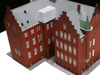
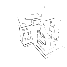
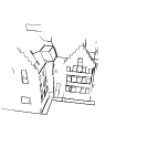
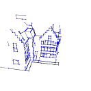
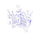
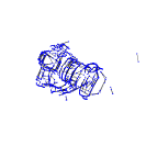
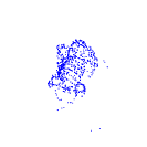
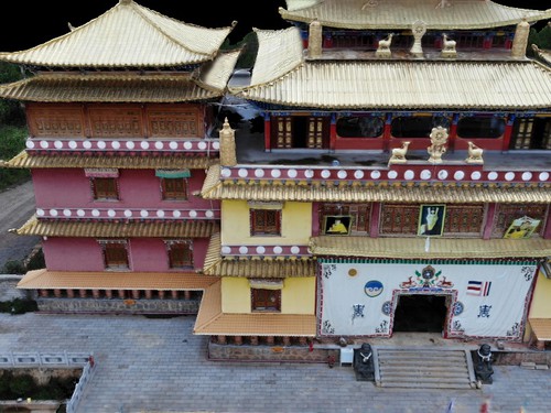
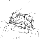
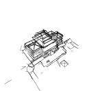
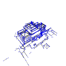
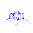
Scene Images	Line3D++@HAWP	NEAT (3D Line Segments)	NEAT (3D Wireframe)	NEAT (3D Junctions)

Figure 3: Quantative comparison between Line3D++@HAWP and our proposed method. We display the two scenes (scan24 and scan105) from DTU (at the top) and the other two scenes (scan1 and scan3) from BlendedMVS (at the bottom). From left to right, we show the scene images, the reconstructed 3D line segments by L3d@HAWP baseline, and our results. For the reconstructed 3D wireframes, we present 3 views to show the results in the view of 3D line segments, 3D wireframes, and 3D junction points, respectively. Video results are in the supplementary materials.

5.2 Main Comparisons

We compare our NEAT approach with three baselines on the scenes from DTU and BlendedMVS datasets, which include both the straight-line dominant scenes and some curve-based ones. In Tab. 1, we quantitatively report the ACCs for both 3D line segments and their junctions (or endpoints), as well as the number of geometric primitives. Compared to the baseline Line3D++@HAWP that takes the same 2D wireframes as input, our NEAT significantly outperforms it in all metrics, which indicates that NEAT is able to yield more accurate and complete 3D reconstruction results than L3D++ for HAWP inputs.

Fig. 3 shows the quantitative comparison results between Line3D++@HAWP and our method on the two real-scene datasets. As is shown, our approach can simultaneously handle both straight-line scenes and complicated ones with curved structures. That is to say, our NEAT is of great potential for the more general purpose of structural scene representation by 3D wireframes.

5.3 Ablation Studies

In our ablation study, two scenes (i.e., DTU-24 and DTU-105) are used as representative cases to discuss our NEAT approach. In the first, we qualitatively show the NEAT lines (i.e., raw output of 3D line segments by querying the NEAT field), the initial reconstruction by binding the queried NEAT lines to global junctions, and the final reconstruction results by the visibility checking. Then, we discuss our NEAT approach in the following two aspects: (1) the parameterization of NEAT Fields and (2) the view dependency issue for junction perceiving.

(a) 6416 lines

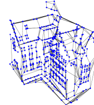
(b) 1165 lines

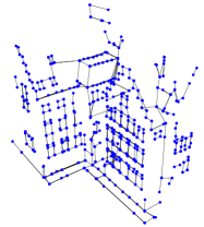
(c) 526 lines

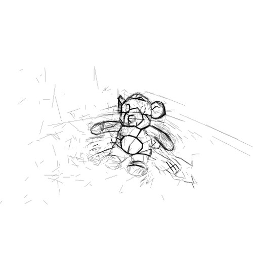
(d) 3792 lines

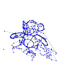
(e) 858 lines

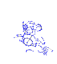
(f) 265 lines

Figure 4: Left: NEAT lines (by coordinate MLP); Middle: initial wireframes (without visibility checking); Right: the final wireframes (with visibility checking) in the right.

The Process of Wireframe Reconstruction.

Fig. 4 shows the three steps for wireframe reconstruction. In the first step, we query all possible 3D line segments from the optimized NEAT field. Then, the queried 3D line segments are binding to the global junctions. In the final step, by leveraging the visibility checking, the unstable 3D line segments are removed from the initial wireframe models. Benefitting from the proposed Global Junction Perceiving module, we largely simplified the way of removing duplicated and unreliable line segments without using either the known 3D points or the complicated line segment matching.

	View Dir.	Clustering	ACC (J)$\downarrow$	ACC (L)$\downarrow$	# Lines	# Junctions
DTU-24	No	No	0.755	0.537	446	520
	Yes	No	0.563	0.472	523	460
	Yes	Yes	0.456	0.420	578	528
DTU-105	No	No	0.575	0.738	252	220
	Yes	No	0.478	0.775	197	175
	Yes	Yes	0.455	0.733	265	204

Table 2: Quantatively evaluation results for ablation studies on the DTU-24 and DTU-105 scenes.

Parameterization of NEAT Fields.

We found that the parameterization of NEAT Fields learning is playing in a vital role in the wireframe reconstruction. Even though our NEAT field aims at representing 3D line segments by the displacement vectors of the 3D points, the localization error in the detected 2D wireframes will possibly lead to some 3D line segments that cannot be well supported by high-quality 2D detection results missing. The information on view direction is a key factor to avoid this issue and yield more complete results. According to Tab. 2, the parameterization without the viewing directions will result in a coarser reconstruction with larger ACC errors for both 3D junctions and line segments while having fewer line segments although the number of global junctions is similar to the final model.

Clustering in Junction Perceiving.

The DBScan [9] clustering is a key factor in accurately perceiving global junctions from the view-dependent coordinate MLP of the NEAT field. To verify this factor, we ablated the DBScan clustering to optimize MLPs on DTU-24 and DTU-105. Quantitatively reported in Tab. 2, although the parameterization of viewing direction largely reduced the ACC errors for both reconstructed junctions and line segments, the number of 3D junctions and line segments is also significantly reduced. When we enable the clustering during optimization, the lower-quality 3D local junctions (from the NEAT field) can be filtered, thus leading to an easy-to-optimize mode to yield more 3D junctions and line segments with fewer reconstruction errors.

5.4 Failure Mode and Limitations

Because our method is built on the top of VolSDF [47], the difficulties for the inside-out scenes for neural surface rendering solutions are inevitable in the current stage. The recent studies [49] that leverages the pre-trained monocular depth and normal maps [8] would overcome those difficulties, but it is out of the scope of this paper. We would leave it in our future work. The quality of 2D wireframe detection would be another key factor leading to the failures. Once the used HAWP model [45] fails to accurately detect wireframes, we cannot accomplish the goal of 3D wireframe reconstruction and parsing. Based on those two points, Fig. 5 provides a representative failure case, which is provided by the ScanNet [7] dataset. Due to the existence of motion blur, although the HAWP model detects the wireframes, the shifted locations with respect to motion blur will lead to many flying 3D line segments from the NEAT fields. Then, by attracting the flying line segments to the global junctions, the visibility checking will filter out many line segments as shown in Fig. 5(c). Even so, the learned global junctions shown in Fig. 5(d) seem to like faithfully learned from the blurry 2D wireframes. One possible reason is that our global design could average the 2D reprojection error during optimization. Such a phenomenon is possible to bring some new perspectives to rethink the relationship between junctions and line segments for the wireframe representation.

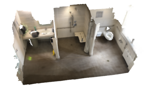
(a) Groundtruth 3D Mesh

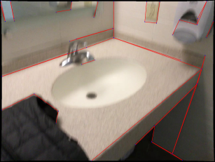
(b) Blur Images and Wireframes

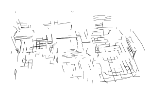
(c) Final Wireframe Model

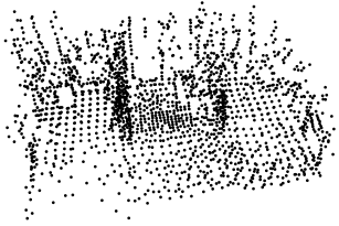
(d) Global 3D Junctions

Figure 5: A Representative Failure Mode on ScanNet.

6 Conclusion

This paper studied the problem of multi-view 3D wireframe parsing (reconstruction) to provide a novel viewpoint for compact 3D scene representation. Building on the basis of the volumetric rendering formulation, we propose a novel NEAT solution that simultaneously learns the coordinate MLPs for the implicit representation of the 3D line segments, and the global junction perceiving (GJP) to explicitly learn global junctions from the randomly-initialized latent arrays in a self-supervised paradigm. Based on new findings, we finally achieve our goal of computing a parsimonious 3D wireframe representation from 2D images and wireframes without considering any heuristic correspondence search for 2D wireframes. To our knowledge, we are the first to achieve multi-view 3D wireframe reconstruction with volumetric rendering. Our proposed novel GJP module opens a door to characterize the scene geometry from 2D supervision in structured point-level 3D representation.

Supplementary Material

The supplementary document is summarized as follows:

• Appx. A gives a summary of the submitted supplementary video.

• Appx. B elaborates on the technical details (introduced in Sec. 3.2 of the main paper)of the wireframe-driven ray sampling and the corresponding rendering results.

• Appx. C supplies the details for the NEAT field learning (introduced in Sec. 4), including the network architecture, visibility checking, and some additional experimental results.

• Appx. D illustrates the difference between 3D wireframe parsing and Line-based 3D reconstruction [14] in additional experiments.

• Appx. E presents the additional experiments on the ABC dataset [18] to discuss the performance given the ground-truth annotations of 3D wireframes.

• Appx. F shows the miscellaneous stuff.

Appendix A Video

In our video https://youtu.be/qtBQYbOpVpc, we first illustrate our key ideas by using a simple object from the ABC dataset as a running example for the learned 3D line segments by NEAT field, the global junction perceiving module, as well as the final 3D wireframe model. Then, we visualize the learned redundant 3D line segments and the optimization process of the global junctions on the DTU-24 as another running example. Finally, the qualitative evaluations on the DTU and BlendedMVS are presented, which are all aligned with the quantitative evaluations of our main paper.

Appendix B Wireframe-driven Ray Sampling

To demonstrate the wireframe-driven ray sampling, we run a set of experiments on the scene 24 from the DTU dataset [1]. Fig. 6 shows the feasibility of optimizing coordinate MLPs by using wireframe-driven ray sampling. As shown in Fig. 6(a), by masking more than 80% pixels out (with a distance threshold of 10 pixels), the optimization of coordinate MLPs also works to result in reasonable results in Fig. 6(b). Apart from the rendering results, we found that the increase in the distance threshold will lead to fewer line segments and junctions. As reported in Tab. 3, when we set the distance threshold to $\tau_{d}=20$, the number of 3D lines and junctions are all decreased even though the ACC errors are also reduced since the pixels far away from line segments may not be related to any line segments. When the distance threshold $\tau_{d}$ is set to $1$, due to the insufficient supervision signals, performance degeneration is observed across all the metrics.

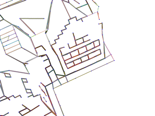
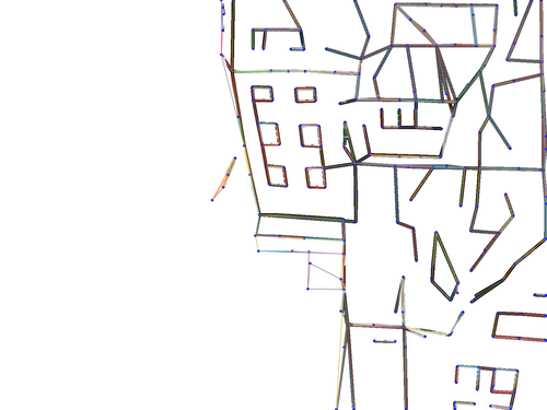
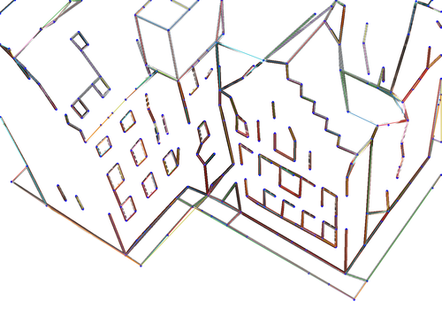
MR: 90.88%	MR: 91.42%	MR: 89.32%
(a). Foreground Pixels defined by 2D wireframes ($\tau_{d}=5$)
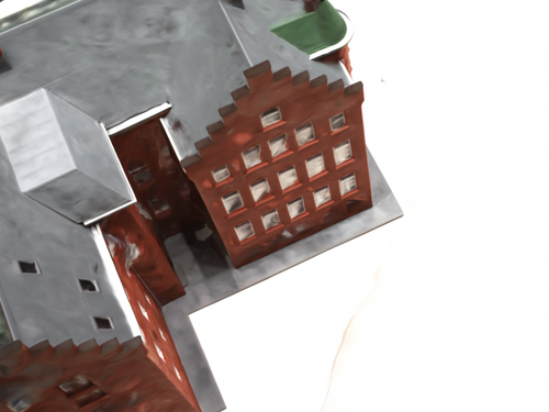
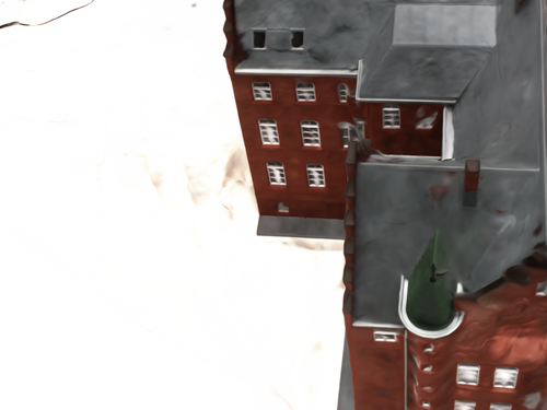
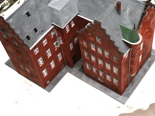
PSNR: 25.46	PSNR: 26.31	PSNR: 21.37
(b). Rendered Images by NEAT
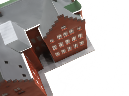
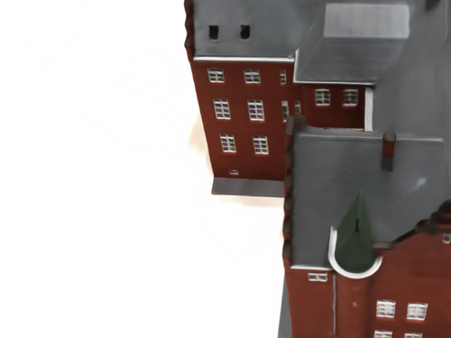
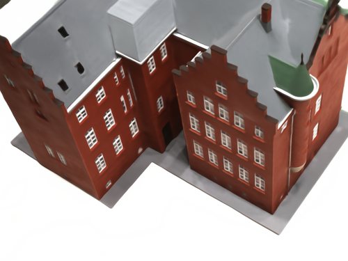
PSNR: 27.40	PSNR: 28.52	PSNR: 26.62
(c). Rendered Images by VolSDF [47]

Figure 6: A comparison for volumetric rendering learned from wireframe-related rays (pixels) vs. the vanilla ray sampling. In (a), we show the 2D line segments detected by HAWPv3 [45] and the used foreground pixels in each view. “MR” denotes the mask ratio (the number of foreground pixels among all the pixels). In (b), we show the corresponding views rendered by NEAT that are learned by the foreground pixels in (a). In the bottom (c), we show the rendered images by VolSDF [47] as the reference. In (b) and (c), the PSNR values are marked at the bottom for each view.

	ACC-J$\downarrow$	ACC-L$\downarrow$	#Lines	#Junctions	MR	PSNR
$\tau_{d}=1$	0.665	0.5374	589	402	97.49%	17.79
$\tau_{d}=5$	0.5368	0.4558	578	528	89.70%	21.55
$\tau_{d}=20$	0.3997	0.3655	430	366	66.10%	24.68

Table 3: The influence of wireframe reconstruction results from different distance thresholds. The larger $\tau_{d}$ value is, the more line segments are involved in the optimization/learning.

Appendix C Details of NEAT Field Learning

C.1 Additional Implementation Details

Network Architecture.

The coordinate MLPs used in our NEAT approach are derived from VolSDF [47], which contains three coordinate MLPs for SDF, the radiance field, and the NEAT field. For the MLP of SDF, it contains 8 layers with hidden layers of width 256 and a skip connection from the input to the 4th layer. The radiance field and the NEAT field share the same architecture with 4 layers with hidden layers of width 256 without skip connections. The proposed global junction perceiving (GJP) module contains two hidden layers and one decoding layer as described in the code snippets of Sec.  1 in our main paper.

Hyperparameters.

The distance threshold $\tau_{d}$ about the foreground pixel (ray) generation is set to $5$ by default. For the number of global junctions (i.e., the size of the latent), we set it to $1024$ on the DTU and BlendedMVS datasets. When the scene scale is larger (e.g., a scene from ScanNet mentioned in Fig. 5 of the main paper), the number of global junctions is set to $2048$. For DBScan [9], we use the implementation from sklearn package, set the epsilon (for the maximum distance between two samples) to 0.01 and the number of samples (in a neighborhood for a point to be considered as a core point) to 2.

The Definition of ACC Metric.

We follow the official evaluation protocol of the DTU dataset [1] to compute the reconstruction accuracy (ACC), which is defined to

$${\rm ACC}=\underset{\begin{subarray}{c}\mathbf{p}\in P\end{subarray}}{\mathrm{mean}}\left(\min_{\mathbf{p}^{*}\in P^{*}}\left\|\mathbf{p}-\mathbf{p}^{*}\right\|\right),$$ (9)

where $P$ and $P^{*}$ are the point clouds sampled from the predictions and the ground truth mesh. Because we pursue the parsimonious 3D representation, we did not use the reconstruction completeness (i.e., COMP) as the metric for evaluation. Instead, we use the number of 3D junctions and line segments to show the completeness of the reconstructed 3D wireframes.

C.2 Visibility Checking

As mentioned in Sec. 4.3 of the main paper, the visibility checking is leveraged to filter out the incorrect wireframe edges (i.e., 3D line segments). Considering the fact that 2D detection results by HAWPv3 [45] are not accurate enough, we would like to use a relaxed criterion to check if a 3D line segment is visible in $1$ view, and use the visibility count over all the queried views to filter out the incorrect 3D line segments. Given a 2D line segment $\ddot{l}_{p}=(\mathbf{x}_{1}^{p},\mathbf{x}_{2}^{p})$ by projecting a 3D line segment $\ddot{L}$ in the queried view with camera parameters ($K$, $R$, $T$), we define the visibility at the queried view by

$$\begin{split}{\rm Vis}(\ddot{l}_{p}|K,R,T)=\min_{\ddot{l}_{q}}(\left\|\mathbf{x}_{1}^{p}-\mathbf{x}_{1}^{q}\right\|_{2}^{2}+\left\|\mathbf{x}_{2}^{p}-\mathbf{x}_{2}^{q}\right\|_{2}^{2},\\ \left\|\mathbf{x}_{1}^{p}-\mathbf{x}_{2}^{q}\right\|_{2}^{2}+\left\|\mathbf{x}_{2}^{p}-\mathbf{x}_{1}^{q}\right\|_{2}^{2})<\tau_{v},\end{split}$$ (10)

where $\ddot{l}_{q}$ are the detected line segments in the queried view. By summing the visibility across viewpoints in

$${\rm Vis}(\ddot{L})=\sum_{K,R,T}{\rm Vis}(\ddot{l}_{p}|K,R,T),$$ (11)

the 3D line segments that are visible in less than $\tau_{\rm ck}\in\mathbb{Z}^{+}$ will be discarded. In our implementation, $\tau_{\rm ck}$ is set to $5$ and $\tau_{v}$ is set to $100$ for all scenes. More careful tuning of $\tau_{\rm ck}$ and $\tau_{v}$ would improve the final performance, but it is not our main scope.

C.3 SDF-based 3D Junction Refinement

To demonstrate the effectiveness of the junction refinement by the SDF, we provide an ablation study to obtain the 3D wireframe models with and without the SDF-based refinement in Tab. 4, which shows that the junction refinement is necessary to obtain significantly better results.

	NEAT (Final)				NEAT (w/o SDF-based Refinement)
Scan	ACC-J $\downarrow$	ACC-L $\downarrow$	#Lines	#Junctions	ACC-J $\downarrow$	ACC-L $\downarrow$	#Lines	#Junctions
DTU Dataset
Avg.	0.4842	0.5368	476.8	353.1	0.8827	0.6915	508.2	376.7
16	0.5340	0.5241	566	432	0.7752	0.6311	575	443
17	0.6262	0.5556	661	452	0.8596	0.6562	716	488
18	0.4695	0.4555	544	403	0.7328	0.6467	600	434
19	0.3758	0.4439	493	367	0.6739	0.5411	517	408
21	0.5659	0.4873	587	437	0.7417	0.5955	604	455
22	0.4269	0.4645	533	413	0.7392	0.6174	564	440
23	0.4864	0.5415	656	493	0.7567	0.6662	666	502
24	0.4558	0.4196	578	528	0.7284	0.5539	606	448
37	0.6613	0.7512	185	168	1.1781	1.0084	238	229
40	0.3931	0.4280	587	267	0.9160	0.6290	519	286
65	0.3606	0.6367	67	73	1.0392	0.7680	86	95
105	0.4545	0.7333	265	204	1.4516	0.9842	407	292
BlendedMVS Dataset
Avg.	0.1553	0.1645	902	552.4	0.2659	0.2182	934	595.4
1	0.0303	0.0414	847	574	0.0565	0.0483	874	592
2	0.1620	0.1589	508	354	0.2402	0.1925	559	419
3	0.1787	0.1791	1193	657	0.2372	0.2063	1198	676
4	0.2638	0.3028	867	551	0.5322	0.4454	871	614
5	0.1418	0.1401	1095	626	0.2636	0.1986	1168	676

Table 4: An Ablation study of the SDF-based 3D Junction Refinement on the DTU and BlendedMVS datasets for the reconstructed 3D wireframes. ACC-J and ACC-L are the evaluation for junctions and line segments.

	NEAT (Ours)					Line3D++@HAWP				Line3D++M				Line3D++O
Scan	ACC-J$\downarrow$	ACC-L$\downarrow$	#Junctions	#Lines	Avg. Length	ACC-J	ACC-L	#Lines	Avg. Length	ACC-J	ACC-L	#Lines	Avg. Length	ACC-J	ACC-L	#Lines	Avg. Length
16	0.5340	0.5241	432	566	20.73	0.7957	0.6991	388	19.65	0.6215	0.5602	821	20.13	0.4705	0.4388	3996	9.25
17	0.6262	0.5556	452	661	21.94	0.8816	0.7778	395	21.99	0.6967	0.6254	838	23.37	0.4731	0.4457	4485	10.16
18	0.4695	0.4555	403	544	22.90	0.7894	0.7531	305	21.63	0.6232	0.5714	843	24.78	0.5061	0.4841	4329	10.10
19	0.3758	0.4439	367	493	25.32	0.6815	0.6702	301	24.64	0.5540	0.5272	782	21.70	0.3828	0.3786	3940	8.93
21	0.5659	0.4873	437	587	26.39	0.9064	0.7954	330	23.03	0.6615	0.6064	883	25.38	0.4992	0.4635	4536	11.26
22	0.4269	0.4645	413	533	19.83	0.7494	0.7078	328	19.56	0.6401	0.5867	750	22.14	0.4446	0.4059	4151	9.57
23	0.4864	0.5415	493	656	24.11	0.8005	0.7357	320	24.28	0.7443	0.6877	885	26.32	0.4930	0.4502	4959	10.38
24	0.4558	0.4196	528	578	23.12	0.7940	0.6807	366	22.84	0.6724	0.6002	696	21.41	0.4737	0.4445	4573	8.39
37	0.6613	0.7512	168	185	28.48	1.1796	1.0285	60	30.16	1.0026	0.9727	189	21.12	0.7652	0.6917	872	8.89
40	0.3931	0.4280	267	587	44.48	0.8486	0.6876	83	37.69	0.5325	0.4886	184	14.28	0.2944	0.2896	932	4.84
65	0.3606	0.6367	73	67	24.02	1.1008	1.0695	23	20.86	0.6428	0.5495	260	11.58	0.4112	0.4112	973	5.73
105	0.4545	0.7333	204	265	23.71	1.2957	1.0286	61	26.16	0.7222	0.6033	225	13.31	0.4392	0.4059	824	6.06
avg.	0.4842	0.5368	353.1	476.8	25.42	0.9019	0.8028	246.7	24.37	0.6762	0.6149	613.0	20.5	0.4711	0.4425	3214.2	8.6300

Table 5: Evaluation Results on the DTU dataset for the reconstructed 3D wireframe and line segments for NEAT (Ours), Line3D++@HAWP, Line3D++M and Line3D++O. For the reconstruction accuracy ACC-J of junctions (or endpoints) and ACC-L of the line segments, we mark the best and the second-best numbers in bold and underline, respectively.

Appendix D NEAT vs. Line3D++

In this section, we present a more comprehensive comparison between our NEAT and Line3D++ [14]. Note that the original design of Line3D++ [14] favors high-resolution input images to obtain more 2D small-length line segments, we set up two additional baselines, Line3D++O and Line3D++M to indicate the original version and the modified version, respectively. In the modified version Line3D++M, we resize the input images into $512\times 512$ as what it did in HAWPv3 [45] for the detection.

Tab. 5 reports the evaluation results for NEAT and the three baselines of Line3D++ [14]. When comparing our proposed NEAT with Line3D++M that detect wireframes/line segments in images with the size of $512\times 512$, the overall ACC errors for 3D junctions and 3D line segments are significantly reduced by 71.6% and 87.3% relative improvements, respectively. As for the vanilla Line3D++ (i.e., Line3D++O), it obtains the best reconstruction accuracy with small-length line segments. Compared to all baselines, the average length of the reconstructed 3D line segments by our NEAT is 25.42, significantly longer than the LSD-based baselines. Although the average length of Line3D++@HAWP is similar to ours, its reconstruction error is also larger than other approaches.

Appendix E Experiments on the ABC Dataset

Images
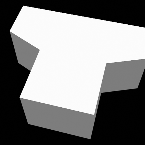
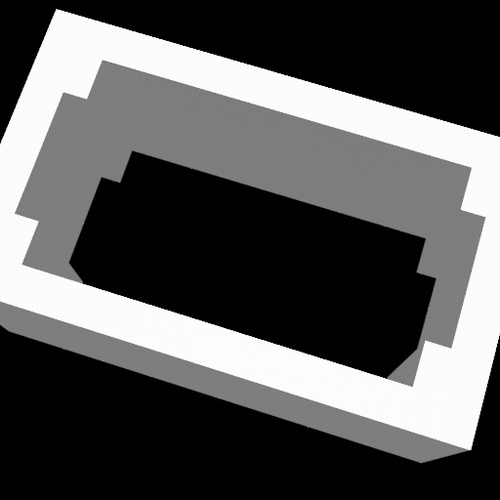
NEAT (Ours)
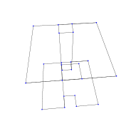
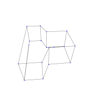
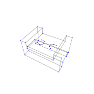
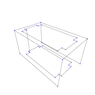
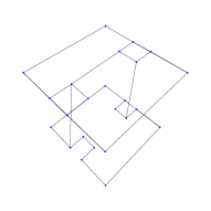
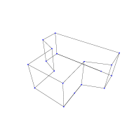
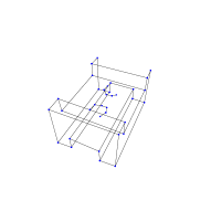
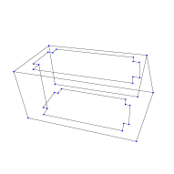
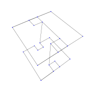
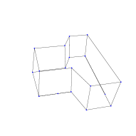
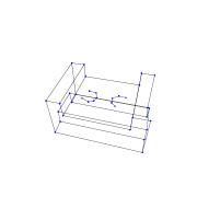
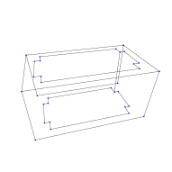
Ideal Baseline

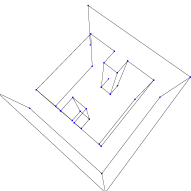
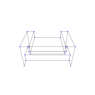
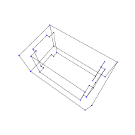
Figure 7: Qualitative Comparisons on ABC objects.

Because the 3D wireframe annotations are very difficult to obtain for real scene images, to better discuss the problem of 3D wireframe reconstruction and analyze our proposed NEAT approach, we conduct experiments on objects from ABC Datasets as it provides 3D wireframe annotations.

Data Preparation.

We use Blender [6] to render 4 objects from the ABC dataset. The object IDs are mentioned in Tab. 6. For each object, we first resize it into a unit cube by dividing the size of the longest side and then moving it to the origin center. Then, we randomly generate 100 camera locations, each of which is distant from the origin by $\sqrt{1.5^{2}+1.5^{2}}\approx 2.1213$ units. The setting of the distance, $\sqrt{1.5^{2}+1.5^{2}}$, is from our early-stage development for the rendering, in which we set a camera at $(0,1.5,1.5)$ location. By setting the cameras to look at the origin $(0,0,0)$, we obtain 100 camera poses. Considering the fact that the ABC dataset is relatively simple, we set the focal length to $60.00$mm to ensure the object is slightly occluded for rendering images. The sensor width and height of the camera in Blender are all set to $32$mm. The ground truth annotations of the 3D wireframe are from the corresponding STEP files. For the simplicity of evaluation, we only keep the straight-line structures and ignore the curvature structures to obtain the ground truth annotations. The rendered images are with the size of $512\times 512$.

Baseline Configuration.

Fig. 7 illustrates the rendered input images for the used four objects. Because the rendered images are textureless and with planar objects, the dependency of those baselines on the correspondence-based sparse reconstruction by SfM systems [32] is hardly satisfied to produce reliable line segment matches for 3D line reconstruction. Accordingly, we set up an ideal baseline instead of using Line3D++ [14] for comparison. Specifically, we first detect the 2D wireframes for the rendered input images and then project the junctions and line segments of the ground-truth 3D wireframe models onto the 2D image plane. For the 2D junctions, if a projected ground-truth junction can be supported by a detected one within $5$ pixels in any view, we keep the ground-truth junction as the reconstructed one in the ideal case. For the 2D line segments, we compute the minimal value for the distance of the two endpoints of a detected line segment to check if it can support a ground-truth 3D line. The threshold is also set to $5$ pixels. Then, we count the number of reconstructed 3D line segments and junctions in such an ideal case.

Evaluation Metrics.

For our method, we compute the precision and recall for the reconstructed 3D junctions and line segments under the given thresholds. Because the objects (and the ground-truth wireframes) are normalized in a unit cube, we set the matching thresholds to $\{0.01,0.02,0.05\}$ for evaluation. For the matching distance of line segments, we use the maximal value of the matching distance between two endpoints to identify if a line segment is successfully reconstructed under the specific distance threshold. For the ideal baseline, we report the number of ground-truth primitives (junctions or line segments), the number of reconstructed primitives, and the reconstruction rate.

Results and Discussion.

Tab. 6 quantitatively summarizes the evaluation results and the statistics on the used scenes. As it is reported, our NEAT approach could accurately reconstruct the wireframes from posed multiview images. The main performance bottleneck of our method comes from the 2D detection results. As shown in the ideal baseline, by projecting the 3D junctions and line segments into the image planes to obtain the ideal 2D detection results, the 2D detection results by HAWPv3 [45] did not perfectly hit all ground-truth annotations. Furthermore, suppose we use the hit (localization error is less than 5 pixels) ground truth for 3D wireframe reconstruction, there is a chance to miss some 3D junctions and more 3D line segments. In this sense, given a relaxed threshold of the reconstruction error for precision and recall computation, our NEAT approach is comparable with the performance of the ideal solution. For the first object (ID 4981), because of the severe self-occlusion, some line segments are not successfully reconstructed for both the ideal baseline and our approach. For object 17078, our NEAT approach reconstructed some parts of the two circles that are excluded from the ground truth, which leads to a relatively low precision rate. Fig. 7 also supported our results.

		Evaluation Results						Ideal Baseline
ID		$P_{0.01}$	$P_{0.02}$	$P_{0.05}$	$R_{0.01}$	$R_{0.02}$	$R_{0.05}$	#GT	# Reconstructed	Recon. Rate
4981	J	0.706	0.765	0.882	0.750	0.812	0.938	32	28	0.875
	L	0.758	0.758	0.758	0.521	0.521	0.521	48	41	0.854
13166	J	0.889	0.889	0.889	1.000	1.000	1.000	16	16	1.000
	L	1.000	1.000	1.000	1.000	1.000	1.000	24	24	1.000
17078	J	0.400	0.629	0.686	0.583	0.917	1.000	24	23	0.958
	L	0.408	0.653	0.714	0.556	0.889	0.972	36	32	0.889
19674	J	0.969	1.000	1.000	0.969	1.000	1.000	32	32	1.000
	L	0.969	1.000	1.000	0.969	1.000	1.000	48	40	0.833

Table 6: Evaluation Results and some Statistics on ABC objects. In each object, we evaluate the precision and recall rates for junctions (J) and line segments (L). For the ideal baseline, we count the number of ground-truth primitives, the number of reconstructed 3D primitives, and the reconstruction rate in the ideal baseline.

Appendix F Miscellaneous

The scene IDs and their MD5 code of the BlendedMVS scenes are:

• Scene-01: 5c34300a73a8df509add216d

• Scene-02: 5b6e716d67b396324c2d77cb

• Scene-03: 5b6eff8b67b396324c5b2672

• Scene-05: 5bf18642c50e6f7f8bdbd492

• Scene-04: 5af28cea59bc705737003253

References

- [1] Henrik Aanæs, Rasmus Ramsbøl Jensen, George Vogiatzis, Engin Tola, and Anders Bjorholm Dahl. Large-scale data for multiple-view stereopsis. Int. J. Comput. Vis., 120(2):153–168, 2016.
- [2] Jonathan T. Barron, Ben Mildenhall, Matthew Tancik, Peter Hedman, Ricardo Martin-Brualla, and Pratul P. Srinivasan. Mip-nerf: A multiscale representation for anti-aliasing neural radiance fields. In IEEE/CVF International Conference on Computer Vision (ICCV), pages 5835–5844, 2021.
- [3] Jonathan T. Barron, Ben Mildenhall, Dor Verbin, Pratul P. Srinivasan, and Peter Hedman. Mip-nerf 360: Unbounded anti-aliased neural radiance fields. In IEEE/CVF Conference on Computer Vision and Pattern Recognition (CVPR), pages 5460–5469, 2022.
- [4] Nicolas Carion, Francisco Massa, Gabriel Synnaeve, Nicolas Usunier, Alexander Kirillov, and Sergey Zagoruyko. End-to-end object detection with transformers. In European Conference on Computer Vision (ECCV), volume 12346, pages 213–229, 2020.
- [5] Manmohan Krishna Chandraker, Jongwoo Lim, and David J. Kriegman. Moving in stereo: Efficient structure and motion using lines. In IEEE/CVF International Conference on Computer Vision (ICCV), pages 1741–1748, 2009.
- [6] Blender Online Community. Blender - a 3D modelling and rendering package. Blender Foundation, Stichting Blender Foundation, Amsterdam, 2018.
- [7] Angela Dai, Angel X. Chang, Manolis Savva, Maciej Halber, Thomas A. Funkhouser, and Matthias Nießner. Scannet: Richly-annotated 3d reconstructions of indoor scenes. In IEEE/CVF Conference on Computer Vision and Pattern Recognition (CVPR), pages 2432–2443, 2017.
- [8] Ainaz Eftekhar, Alexander Sax, Jitendra Malik, and Amir Zamir. Omnidata: A scalable pipeline for making multi-task mid-level vision datasets from 3d scans. In IEEE/CVF International Conference on Computer Vision (ICCV), pages 10766–10776, 2021.
- [9] Martin Ester, Hans-Peter Kriegel, Jörg Sander, and Xiaowei Xu. Density-based spatial clustering of applications with noise. In International Conference on Knowledge Discovery and Data Mining (KDD), volume 240, 1996.
- [10] Xiao Fu, Shangzhan Zhang, Tianrun Chen, Yichong Lu, Lanyun Zhu, Xiaowei Zhou, Andreas Geiger, and Yiyi Liao. Panoptic nerf: 3d-to-2d label transfer for panoptic urban scene segmentation. In International Conference on 3D Vision (3DV), pages 1–11, 2022.
- [11] Lily Goli, Daniel Rebain, Sara Sabour, Animesh Garg, and Andrea Tagliasacchi. nerf2nerf: Pairwise registration of neural radiance fields. In IEEE International Conference on Robotics and Automation (ICRA), 2023.
- [12] Adolfo Guzmán. Decomposition of a visual scene into three-dimensional bodies. In Fall Joint Computer Conference, volume 33, pages 291–304, 1968.
- [13] Richard Hartley and Andrew Zisserman. Multiple View Geometry in Computer Vision. Cambridge university press, 2003.
- [14] Manuel Hofer, Michael Maurer, and Horst Bischof. Efficient 3d scene abstraction using line segments. Comput. Vis. Image Underst., 157:167–178, 2017.
- [15] Andrew Jaegle, Sebastian Borgeaud, Jean-Baptiste Alayrac, Carl Doersch, Catalin Ionescu, David Ding, Skanda Koppula, Daniel Zoran, Andrew Brock, Evan Shelhamer, Olivier J. Hénaff, Matthew M. Botvinick, Andrew Zisserman, Oriol Vinyals, and João Carreira. Perceiver IO: A general architecture for structured inputs & outputs. In International Conference on Learning Representations (ICLR), 2022.
- [16] Andrew Jaegle, Felix Gimeno, Andy Brock, Oriol Vinyals, Andrew Zisserman, and João Carreira. Perceiver: General perception with iterative attention. In International Conference on Machine Learning (ICML), volume 139, pages 4651–4664, 2021.
- [17] Diederik P. Kingma and Jimmy Ba. Adam: A method for stochastic optimization. In International Conference on Learning Representations (ICLR), 2015.
- [18] Sebastian Koch, Albert Matveev, Zhongshi Jiang, Francis Williams, Alexey Artemov, Evgeny Burnaev, Marc Alexa, Denis Zorin, and Daniele Panozzo. ABC: A big CAD model dataset for geometric deep learning. In IEEE/CVF Conference on Computer Vision and Pattern Recognition (CVPR), pages 9601–9611, 2019.
- [19] Harold W Kuhn. The hungarian method for the assignment problem. Naval Research Logistics Quarterly, 2(1-2):83–97, 1955.
- [20] Abhijit Kundu, Kyle Genova, Xiaoqi Yin, Alireza Fathi, Caroline Pantofaru, Leonidas J. Guibas, Andrea Tagliasacchi, Frank Dellaert, and Thomas A. Funkhouser. Panoptic neural fields: A semantic object-aware neural scene representation. In IEEE/CVF Conference on Computer Vision and Pattern Recognition (CVPR), pages 12861–12871, 2022.
- [21] David C. Lee, Martial Hebert, and Takeo Kanade. Geometric reasoning for single image structure recovery. In IEEE/CVF Conference on Computer Vision and Pattern Recognition (CVPR), pages 2136–2143, 2009.
- [22] David Marr. Vision: A computational investigation into the human representation and processing of visual information. MIT press, 2010.
- [23] Ishit Mehta, Manmohan Chandraker, and Ravi Ramamoorthi. A level set theory for neural implicit evolution under explicit flows. In European Conference on Computer Vision (ECCV), volume 13662, pages 711–729, 2022.
- [24] Ben Mildenhall, Pratul P. Srinivasan, Matthew Tancik, Jonathan T. Barron, Ravi Ramamoorthi, and Ren Ng. NeRF: representing scenes as neural radiance fields for view synthesis. In European Conference on Computer Vision (ECCV), volume 12346, pages 405–421, 2020.
- [25] Michael Oechsle, Songyou Peng, and Andreas Geiger. UNISURF: unifying neural implicit surfaces and radiance fields for multi-view reconstruction. In IEEE/CVF International Conference on Computer Vision (ICCV), pages 5569–5579, 2021.
- [26] Adam Paszke, Sam Gross, Francisco Massa, Adam Lerer, James Bradbury, Gregory Chanan, Trevor Killeen, Zeming Lin, Natalia Gimelshein, Luca Antiga, Alban Desmaison, Andreas Köpf, Edward Z. Yang, Zachary DeVito, Martin Raison, Alykhan Tejani, Sasank Chilamkurthy, Benoit Steiner, Lu Fang, Junjie Bai, and Soumith Chintala. Pytorch: An imperative style, high-performance deep learning library. In Advances in Neural Information Processing Systems (NeurIPS), pages 8024–8035, 2019.
- [27] Rémi Pautrat, Daniel Barath, Viktor Larsson, Martin R. Oswald, and Marc Pollefeys. Deeplsd: Line segment detection and refinement with deep image gradients. In IEEE/CVF Conference on Computer Vision and Pattern Recognition (CVPR), 2023.
- [28] Rémi Pautrat, Juan-Ting Lin, Viktor Larsson, Martin R. Oswald, and Marc Pollefeys. SOLD2: self-supervised occlusion-aware line description and detection. In IEEE/CVF Conference on Computer Vision and Pattern Recognition (CVPR), pages 11368–11378, 2021.
- [29] Albert Pumarola, Alexander Vakhitov, Antonio Agudo, Alberto Sanfeliu, and Francesc Moreno-Noguer. PL-SLAM: real-time monocular visual SLAM with points and lines. In IEEE International Conference on Robotics and Automation (ICRA), pages 4503–4508, 2017.
- [30] Yohann Salaün, Renaud Marlet, and Pascal Monasse. Multiscale line segment detector for robust and accurate sfm. In International Conference on Pattern Recognition (ICPR), pages 2000–2005, 2016.
- [31] Cordelia Schmid and Andrew Zisserman. Automatic line matching across views. In IEEE/CVF Conference on Computer Vision and Pattern Recognition (CVPR), pages 666–671, 1997.
- [32] Johannes L. Schönberger and Jan-Michael Frahm. Structure-from-motion revisited. In IEEE/CVF Conference on Computer Vision and Pattern Recognition (CVPR), pages 4104–4113, 2016.
- [33] Johannes L. Schönberger, Enliang Zheng, Jan-Michael Frahm, and Marc Pollefeys. Pixelwise view selection for unstructured multi-view stereo. In European Conference on Computer Vision (ECCV), volume 9907, pages 501–518, 2016.
- [34] Kokichi Sugihara. A necessary and sufficient condition for a picture to represent a polyhedral scene. IEEE Trans. Pattern Anal. Mach. Intell., 6(5):578–586, 1984.
- [35] Christopher Sweeney, Tobias Höllerer, and Matthew A. Turk. Theia: A fast and scalable structure-from-motion library. In ACM International Conference on Multimedia (ACMMM), pages 693–696, 2015.
- [36] Rafael Grompone von Gioi, Jérémie Jakubowicz, Jean-Michel Morel, and Gregory Randall. LSD: A fast line segment detector with a false detection control. IEEE Trans. Pattern Anal. Mach. Intell., 32(4):722–732, 2010.
- [37] Bing Wang, Lu Chen, and Bo Yang. Dm-nerf: 3d scene geometry decomposition and manipulation from 2d images. In International Conference on Learning Representations (ICLR), 2023.
- [38] Peng Wang, Lingjie Liu, Yuan Liu, Christian Theobalt, Taku Komura, and Wenping Wang. Neus: Learning neural implicit surfaces by volume rendering for multi-view reconstruction. In Advances in Neural Information Processing Systems (NeurIPS), pages 27171–27183, 2021.
- [39] Qiuyuan Wang, Zike Yan, Junqiu Wang, Fei Xue, Wei Ma, and Hongbin Zha. Line flow based simultaneous localization and mapping. IEEE Trans. Robotics, 37(5):1416–1432, 2021.
- [40] Changchang Wu. Towards linear-time incremental structure from motion. In International Conference on 3D Vision (3DV), pages 127–134, 2013.
- [41] Qianyi Wu, Xian Liu, Yuedong Chen, Kejie Li, Chuanxia Zheng, Jianfei Cai, and Jianmin Zheng. Object-compositional neural implicit surfaces. In European Conference on Computer Vision (ECCV), volume 13687, pages 197–213, 2022.
- [42] Nan Xue, Song Bai, Fudong Wang, Gui-Song Xia, Tianfu Wu, and Liangpei Zhang. Learning attraction field representation for robust line segment detection. In IEEE/CVF Conference on Computer Vision and Pattern Recognition (CVPR), pages 1595–1603, 2019.
- [43] Nan Xue, Song Bai, Fudong Wang, Gui-Song Xia, Tianfu Wu, Liangpei Zhang, and Philip H. S. Torr. Learning regional attraction for line segment detection. IEEE Trans. Pattern Anal. Mach. Intell., 43(6):1998–2013, 2021.
- [44] Nan Xue, Tianfu Wu, Song Bai, Fudong Wang, Gui-Song Xia, Liangpei Zhang, and Philip H. S. Torr. Holistically-attracted wireframe parsing. In IEEE/CVF Conference on Computer Vision and Pattern Recognition (CVPR), pages 2785–2794, 2020.
- [45] Nan Xue, Tianfu Wu, Song Bai, Fu-Dong Wang, Gui-Song Xia, Liangpei Zhang, and Philip H.S. Torr. Holistically-attracted wireframe parsing: From supervised to self-supervised learning. arXiv:2210.12971, 2022.
- [46] Yao Yao, Zixin Luo, Shiwei Li, Jingyang Zhang, Yufan Ren, Lei Zhou, Tian Fang, and Long Quan. Blendedmvs: A large-scale dataset for generalized multi-view stereo networks. In IEEE/CVF Conference on Computer Vision and Pattern Recognition (CVPR), pages 1787–1796, 2020.
- [47] Lior Yariv, Jiatao Gu, Yoni Kasten, and Yaron Lipman. Volume rendering of neural implicit surfaces. In Advances in Neural Information Processing Systems (NeurIPS), 2021.
- [48] Lior Yariv, Yoni Kasten, Dror Moran, Meirav Galun, Matan Atzmon, Ronen Basri, and Yaron Lipman. Multiview neural surface reconstruction by disentangling geometry and appearance. In Advances in Neural Information Processing Systems (NeurIPS), 2020.
- [49] Zehao Yu, Songyou Peng, Michael Niemeyer, Torsten Sattler, and Andreas Geiger. Monosdf: Exploring monocular geometric cues for neural implicit surface reconstruction. In Advances in Neural Information Processing Systems (NeurIPS), 2022.
- [50] Yichao Zhou, Haozhi Qi, and Yi Ma. End-to-end wireframe parsing. In IEEE/CVF International Conference on Computer Vision (ICCV), pages 962–971, 2019.
- [51] Yichao Zhou, Haozhi Qi, Yuexiang Zhai, Qi Sun, Zhili Chen, Li-Yi Wei, and Yi Ma. Learning to reconstruct 3d manhattan wireframes from a single image. In IEEE/CVF International Conference on Computer Vision (ICCV), pages 7697–7706, 2019.