Personalized Privacy Amplification via Importance Sampling

Abstract

We examine the privacy-enhancing properties of importance sampling. In importance sampling, selection probabilities are heterogeneous and each selected data point is weighted by the reciprocal of its selection probability. Due to the heterogeneity of importance sampling, we express our results within the framework of personalized differential privacy. We first consider the general case where an arbitrary personalized differentially private mechanism is subsampled with an arbitrary importance sampling distribution and show that the resulting mechanism also satisfies personalized differential privacy. This constitutes an extension of the established privacy amplification by subsampling result to importance sampling. Then, for any fixed mechanism, we derive the sampling distribution that achieves the optimal sampling rate subject to a worst-case privacy constraint. Empirically, we evaluate the privacy, efficiency, and accuracy of importance sampling on the example of $k$-means clustering.

1 Introduction

When deploying machine learning models in practice, two central challenges are the efficient handling of large data sets and the protection of user privacy. A common approach to the former challenge is subsampling, i.e., performing demanding computations only on a subset of the data. Here, importance sampling can improve the efficiency of subsampling by assigning higher sampling probabilities to data points that are more informative for the task at hand, while still retaining an unbiased estimate. For instance, importance sampling is commonly used to construct coresets, that is, subsets whose loss function value is provably close to the loss of the full data set, see, e.g., Bachem et al. (2018). For the latter challenge, differential privacy (Dwork et al., 2006b) offers a framework for publishing trained models in a way that respects the individual privacy of every user.

Differential privacy and subsampling are related via the concept of privacy amplification by subsampling (Kasiviswanathan et al., 2008; Balle et al., 2018), which states, loosely speaking, that subsampling with probability $p$ improves the privacy guarantees of a subsequently run differentially private algorithm by a factor of approximately $p$. A typical application of this result involves re-scaling the query by a factor of $1/p$ to offset the sampling bias, hence approximately canceling out the privacy amplification, but keeping the efficiency gain. It forms the theoretical foundation for many practical applications of differential privacy, such as differentially private stochastic gradient descent (Bassily et al., 2014). So far, privacy amplification by subsampling has been analyzed primarily in the uniform setting where each data point is sampled with the same probability.

We extend this analysis to the case of importance sampling, where each data point is sampled with a probability that depends on the data point itself and is weighted to produce an unbiased estimate. The primary motivation for importance sampling is that data points that induce the highest privacy loss are typically also the most informative for the task at hand. At first, it might seem that this puts privacy and utility at odds with each other. This intuition stems from thinking of subsampling as lowerering the privacy loss of the mechanism. However, when the sampled point is re-weighted by $1/p$, the privacy loss is, in fact, increased for typical mechanisms. Thus, by coupling the sampling probabilities to the individual privacy loss and/or a suitable measure of “informativeness”, we can improve the privacy and accuracy of the subsampled mechanism simultaneously. The primary challenges in this regard are to (i) account for the privacy leakage of the sampling probability itself and to (ii) ensure it can be computed efficiently. We propose two approaches that address these challenges, one based on equalizing the individual privacy losses and the other based on coresets. In our experiments, both appraoches achieve improved trade-offs between privacy, efficiency, and accuracy compared to uniform subsampling. The improvement is particularly pronounced in the medium-to-low privacy regime where uniform subsampling fails to provide meaningful privacy improvement. One practical implication is that importance sampling can be used effectively to subsample the data set once at the beginning of the computation, while uniform subsampling typically requires repeated subsampling at each iteration.

Specifically, we make the following contributions:

• We begin with a general amplification result that quantifies the privacy guarantee of an arbitrary mechanism when subsampled via importance sampling with an arbitrary distribution. We express this result within the framework of personalized differential privacy (Jorgensen et al., 2015; Ebadi et al., 2015; Alaggan et al., 2016), which allows us to quantify the privacy individually for each data point. This constitutes a natural extension of the established amplification results for uniform subsampling (Kasiviswanathan et al., 2008; Balle et al., 2018).

• Next, we describe two approaches for deriving sampling probabilites, each permitting a tight privacy analysis and efficient computation. The first approach is based on coupling the individual probabilities to the individual privacy losses. This approach optimizes the privacy-efficiency trade-off by minimizing the expected sample size subject to a worst-case (i.e., non-personalized) privacy constraint for a given mechanism. We provide an efficient algorithm that finds the optimal distribution numerically. The second approach is based on coupling the selection probability to a measure of “informativeness” that is used in the coreset literature.

• We evaluate the proposed approaches on a large-scale differentially private $k$-means clustering task on a variety of data sets. We compare both approaches to uniform sampling in terms of efficiency, privacy, and accuracy. We find that both approaches consistently outperform uniform sampling and provide meaningful privacy improvements even in the medium-to-low privacy regime. The results are consistent across data sets and are particularly pronounced for small sample sizes.

2 Preliminaries

We begin by stating the necessary concepts that also introduce the notation used in this paper. We denote by $\mathcal{X}\subseteq\mathbb{R}^{d}$ the set of all possible data points. A data set $\mathcal{D}$ is a finite subset of $\mathcal{X}$. We denote by $\mathcal{B}_{d,p}(r)=\{\mathbf{x}\in\mathbb{R}^{d}\mid\|\mathbf{x}\|_{p}\leq r\}$ the $\ell_{p}$-norm ball of radius $r$ in $d$ dimensions. When the dimension is clear from context, we omit the subscript $d$ and write $\mathcal{B}_{p}(r)$.

Differential Privacy.  Differential privacy (DP) is a formal notion of privacy stating that the output of a data processing method should be robust, in a probabilistic sense, to changes in the data set that affect individual data points. It was introduced by Dwork et al. (2006b) and has since become a standard tool for privacy-preserving data analysis (Ji et al., 2014). The notion of robustness is qualified by two parameters, $\epsilon\geq 0$ and $\delta\geq 0$, that relate to the error rate of any adversary that tries to infer whether a particular data point is present in the data set (Kairouz et al., 2015; Dong et al., 2019). Differential privacy is based on the formal notion of indistinguishability.

Definition 2.1 ($(\epsilon,\delta)$-indistinguishability).

Let $\epsilon\geq 0$ and $\delta\geq 0$. Two distributions $P,Q$ on a space $\mathcal{Y}$ are $(\epsilon,\delta)$-indistinguishable if $P(Y)\leq e^{\epsilon}Q(Y)+\delta$ and $Q(Y)\leq e^{\epsilon}P(Y)+\delta$ for all measurable $Y\subseteq\mathcal{Y}$.

Definition 2.2 ($(\epsilon,\delta)$-DP).

A randomized mechanism $\mathcal{M}\colon\mathcal{X}\to\mathcal{Y}$ is said to be $(\epsilon,\delta)$-differentially private ($(\epsilon,\delta)$-DP) if, for all neighboring data sets $\mathcal{D},\mathcal{D}^{\prime}\subseteq\mathcal{X}$, the distributions of $\mathcal{M}(\mathcal{D})$ and $\mathcal{M}(\mathcal{D}^{\prime})$ are $(\epsilon,\delta)$-indistinguishable. For $\delta=0$ we say $\mathcal{M}$ is $\epsilon$-DP. Two data sets $\mathcal{D},\mathcal{D}^{\prime}$ are neighboring if $\mathcal{D}=\mathcal{D}^{\prime}\cup\{\mathbf{x}\}$ or $\mathcal{D}^{\prime}=\mathcal{D}\cup\{\mathbf{x}\}$ for some $\mathbf{x}\in\mathcal{X}$.

Formally, we consider a randomized mechanism as a mapping from a data set to a random variable. Differential privacy satisfies a number of convenient analytical properties, including closedness under post-processing (Dwork et al., 2006b), composition (Dwork et al., 2006b, a, 2010; Kairouz et al., 2015), and sampling (Kasiviswanathan et al., 2008; Balle et al., 2018). The latter is called privacy amplification by subsampling.

Proposition 2.3 (Privacy Amplification by Subsampling).

Let $\mathcal{D}$ be a data set of size $n$, $\mathcal{S}$ be a subset of $\mathcal{D}$ where every $\mathbf{x}$ has a constant probability $p$ of being independently sampled, i.e., $q(\mathbf{x})=p\in(0,1]$, and $\mathcal{M}$ be a $(\epsilon,\delta)$-DP mechanism. Then, $\mathcal{M}(\mathcal{S})$ satisfies $(\epsilon^{\prime},\delta^{\prime})$-DP for $\epsilon^{\prime}=\log\mathopen{}\mathclose{{}\left(1+\mathopen{}\mathclose{{}\left(\exp(\epsilon)-1}\right)p}\right)$ and $\delta^{\prime}=p\delta$.

In the case of heterogeneous sampling probabilities $p_{1},\ldots,p_{n}$, the privacy amplification scales with $\max_{i}p_{i}$ instead of $p$. It is important to note that this only provides meaningful privacy amplification if $\epsilon$ is sufficiently small. For $\epsilon>1$, we only have $\epsilon^{\prime}\approx\epsilon-\log(1/p)$.

Personalized Differential Privacy.  In many applications, the privacy loss of a mechanism is not uniform across the data set. This heterogeneity can be captured by the notion of personalized differential privacy (PDP) (Jorgensen et al., 2015; Ebadi et al., 2015; Alaggan et al., 2016).

Definition 2.4 (Personalized differential privacy).

Let $\epsilon\colon\mathcal{X}\to\mathbb{R}_{\geq 0}$. A mechanism $\mathcal{M}:\mathcal{X}\to\mathcal{Y}$ is said to satisfy $\epsilon$-personalized differential privacy ($\epsilon$-PDP) if, for all data sets $\mathcal{D}$ and differing points $\mathbf{x}\in\mathcal{X}$, the distributions of $\mathcal{M}(\mathcal{D})$ and $\mathcal{M}(\mathcal{D}\cup\{\mathbf{x}\})$ are $\epsilon(\mathbf{x})$-indistinguishable. We call the function $\epsilon(\cdot)$ a PDP profile of $\mathcal{M}$.

Importance Sampling.  In learning problems, the (weighted) objective function that we optimize is often a sum over per-point losses, i.e., $\phi_{\mathcal{D}}=\sum_{\mathbf{x}\in\mathcal{D}}w(\mathbf{x})\ell(\mathbf{x})$. Here, we typically have $w(\mathbf{x})=1$ $\forall\mathbf{x}\in\mathcal{D}$ for the full data. Uniformly subsampling a data set yields an unbiased estimation of the mean. A common way to improve upon uniform sampling is to skew the sampling towards important data points while retaining an unbiased estimate of the objective function. Let $q$ be an importance sampling distribution on $\mathcal{D}$ which we use to sample a subset $\mathcal{S}$ of $m\ll n$ points and weight them with $w(\mathbf{x})=(mq(\mathbf{x}))^{-1}$. Then, the estimation of the objective function is unbiased, i.e., $\mathbb{E}_{\mathcal{S}}\mathopen{}\mathclose{{}\left[\phi_{\mathcal{S}}}\right]=\phi_{\mathcal{D}}$.

3 Privacy Amplification via Importance Sampling

In this section, we present our theoretical contributions on the amplification of personalized differential privacy via importance sampling. We first give a general amplification result in terms of PDP. Then, we describe how to construct sampling distributions that achieve a given DP guarantee with minimal sample size efficiently. We conclude with a numerical example that illustrates the aforementioned results for the Laplace mechanism. We defer the proofs to Appendix D.

General Sampling Distributions.  We begin by introducing the sampling strategy we use throughout the paper. It is a weighted version of the Poisson sampling strategy described in Proposition 2.3. We refer to it as Poisson importance sampling.

Definition 3.1 (Poisson Importance Sampling).

Let $q\colon\mathcal{X}\to[0,1]$ be a function, and $\mathcal{D}=\{\mathbf{x}_{1},\ldots,\mathbf{x}_{n}\}\subseteq\mathcal{X}$ be a data set. A Poisson importance sampler for $q$ is a randomized mechanism $S_{q}(\mathcal{D})=\{(w_{i},\mathbf{x}_{i})\mid\gamma_{i}=1\}$, where $w_{i}=1/q(\mathbf{x}_{i})$ are weights and $\gamma_{1},\ldots,\gamma_{n}$ are independent Bernoulli variables with parameters $p_{i}=q(\mathbf{x}_{i})$.

The function definition of $q$ should be considered public information, i.e., fixed before observing the data set. Note that $q$ is not a probability distribution over $\mathbf{x}$, but simply any function that assigns a number between 0 and 1 to each data point. The expected sample size is $\mathbb{E}[|S_{q}(\mathcal{D})|]=\sum_{i=1}^{n}q(\mathbf{x}_{i})$. With this notion in place, we are ready to state the first main result.

Theorem 3.2 (Amplification by Importance Sampling).

Let $\mathcal{M}:[1,\infty)\times\mathcal{X}\to\mathcal{Y}$ be a $\epsilon$-PDP mechanism that operates on weighted data sets, $q\colon\mathcal{X}\to[0,1]$ be a function, and $S_{q}(\cdot)$ be a Poisson importance sampler for $q$. The mechanism $\widehat{\mathcal{M}}=\mathcal{M}\circ S_{q}$ satisfies $\psi$-PDP with

$$\psi(\mathbf{x})=\log\mathopen{}\mathclose{{}\left(1+q(\mathbf{x})\mathopen{}\mathclose{{}\left(e^{\epsilon(w,\mathbf{x})}-1}\right)}\right),$$ (1)

where $w=1/q(\mathbf{x})$.

The sampled PDP profile in Equation 1 closely resembles the privacy amplification result for uniform sampling (Proposition 2.3) with the difference that $\epsilon(w,\mathbf{x})$ depends on $w$ and $\mathbf{x}$. Notably, $\psi$ is not necessarily monotonic in $q(\mathbf{x})$ for this reason. Moreover, $\psi$ is not guaranteed to be bounded, even when $\epsilon(w,\cdot)$ is. For instance, consider a weighted sum with Laplace noise: $\mathcal{M}_{\text{LWS}}(\mathcal{D})=\zeta+\sum_{i=1}^{n}w_{i}f(\mathbf{x}_{i})$, where $\zeta\sim\operatorname{Lap}(0,1)$. The PDP profile of $\mathcal{M}_{\text{LWS}}$ is $\epsilon_{\text{LWS}}(w,\mathbf{x})=w|f(\mathbf{x})|$. If we choose $q(\mathbf{x})\propto|f(\mathbf{x})|^{2}$, the resulting PDP profile $\psi_{\text{LWS}}$ of $\mathcal{M}_{\text{LWS}}\circ S_{q}$ diverges as $f(\mathbf{x})\to 0$. However, as we show in the next subsection, it is always possible to construct a sampling distribution $q$ that allows the PDP profile $\psi$ of $\mathcal{M}\circ S_{q}$ to be bounded. We provide a detailed discussion of monotonicity in Appendix A.

Sampling with optimal privacy-efficiency trade-off.  We now describe how to construct a sampling distribution that achieves a given privacy guarantee with minimal sample size. The motivation for this is two-fold. First, as we have seen in the previous subsection, not all sampling distributions guarantee a bounded PDP profile. By imposing a constant PDP bound as a constraint, we can ensure that the subsampled mechanism satisfies $\epsilon$-DP by design. Second, the subsample size is the primary indicator of the efficiency of mechanism. This is because the computational cost of computing the sampling distribution is negligible compared to the cost of running the mechanism itself.

Minimizing the expected sample size subject to a given $\epsilon^{\star}$-DP constraint can be described as the following optimization problem.

Problem 3.3 (Privacy-optimal sampling).

For a PDP profile $\epsilon\colon[1,\infty)\times\mathcal{X}\to\mathbb{R}_{\geq 0}$, a target privacy guarantee $\epsilon^{\star}$, and a data set $\mathcal{D}\subseteq\mathcal{X}$ of size $n$, we define the privacy-optimal sampling problem as

$$\min_{\mathbf{w}\in\mathbb{R}^{n}}\quad \sum_{i=1}^{n}\frac{1}{w_{i}}$$ (2a)

s.t. $$\log\mathopen{}\mathclose{{}\left(1+\frac{1}{w_{i}}\mathopen{}\mathclose{{}\left(e^{\epsilon(w_{i},\mathbf{x}_{i})}-1}\right)}\right)\leq\epsilon^{\star}, \forall i,$$ (2b)

$$w_{i}\geq 1, \forall i.$$ (2c)

The constraint in Equation (2b) captures the requirement that $\psi$ should be bounded by $\epsilon^{\star}$ for all $\mathbf{x}\in\mathcal{X}$, and the constraint in Equation (2c) ensures that $1/w_{i}$ is a probability. Note that, unless we make assumptions on the function $\epsilon$ and the target $\epsilon^{\star}$, the problem is not guaranteed to have a solution. First, if $\epsilon^{\star}$ is too small, the constraint in Equation (2b) might be infeasible for some $\mathbf{x}_{i}$. Second, Equation (2b) might reach equality infinitely often if the left hand-side oscillates, e.g., if $\epsilon(\cdot,\mathbf{x})$ is piecewise constant. Fortunately, under mild assumptions about $\epsilon(\cdot,\cdot)$ and $\epsilon^{\star}$, the problem is guaranteed to have a unique solution, and can be solved separately for each $\mathbf{x}\in\mathcal{D}$.

Assumption 3.4.

For all $\mathbf{x}\in\mathcal{X}$, $\epsilon^{\star}\geq\epsilon(1,\mathbf{x})$.

Assumption 3.5.

For all $\mathbf{x}\in\mathcal{X}$, there is a constant $v_{\mathbf{x}}\geq 1$ such that $\epsilon(w,\mathbf{x})>\log(1+w(e^{\epsilon^{\star}}-1))$ for all $w\geq v_{\mathbf{x}}$.

Assumption 3.4 ensures that the feasible region is non-empty, because $w_{1}=w_{2}=\cdots=w_{n}=1$ always satisfies the constraints, while Assumption 3.5 essentially states that, asymptotically, $\epsilon$ should grow at least logarithmically fast with $w$, ensuring that the feasible region is bounded. The second main result is as follows.

Theorem 3.6.

Let Assumptions 3.4 and 3.5 be satisfied. There is a data set-independent function $w\colon\mathcal{X}\to[1,\infty)$, such that, for all data sets $\mathcal{D}\subseteq\mathcal{X}$, Problem 3.3 has a unique solution $w^{\star}(\mathcal{D})=(w^{\star}_{1}(\mathcal{D}),\ldots,w_{n}^{\star}(\mathcal{D}))$ of the form $w_{i}^{\star}(\mathcal{D})=w(\mathbf{x}_{i})$. Furthermore, let $\mathcal{M}$ be a mechanism that admits the PDP profile $\epsilon$ and $S_{q}$ be a Poisson importance sampler for $q(\mathbf{x})=1/w(\mathbf{x})$. Then, $\mathcal{M}\circ S_{q}$ satisfies $\epsilon^{\star}$-DP.

We approach Problem 3.3 by reducing it to a scalar root-finding problem. For that, we introduce Assumption 3.7 which is slightly stronger than Assumption 3.5.

Assumption 3.7.

The function $\epsilon(w,\mathbf{x})$ is differentiable w.r.t. $w$ and $\exp\circ\,\epsilon$ is $\mu_{\mathbf{x}}$-strongly convex in $w$ for all $\mathbf{x}$.

Algorithm 1 Privacy-optimal importance weights

  Input: Data set $\mathcal{D}=\{\mathbf{x}_{1},\ldots,\mathbf{x}_{n}\}$, target privacy guarantee $\epsilon^{\star}>0$, PDP profile $\epsilon$, its derivative $\epsilon^{\prime}$ wrt $w$, and strong convexity constants $\mu_{1},\ldots,\mu_{n}$

  Output: Importance weights $w_{1},\ldots,w_{n}$

  for $i=1,\ldots,n$ do

     Define $g_{i}(w)=\frac{1}{w}\mathopen{}\mathclose{{}\left(e^{\epsilon(w,\mathbf{x}_{i})}-1}\right)-\mathopen{}\mathclose{{}\left(e^{\epsilon^{\star}}-1}\right)$

     $\bar{v}_{i}\leftarrow\min\{e^{\epsilon(1,\mathbf{x}_{i})}+\mu_{i}/2,\ \epsilon^{\prime}(1,\mathbf{x}_{i})e^{\epsilon(1,\mathbf{x}_{i})}+1\}$

     $b_{i}\leftarrow 2(e^{\epsilon^{\star}}-\bar{v}_{i})/\mu_{i}+1$

     if $\epsilon(1,\mathbf{x}_{i})=\epsilon^{\star}$ and $\epsilon^{\prime}(1,\mathbf{x}_{i})<0$ then

        $w_{i}\leftarrow$ Bisect $g_{i}$ with initial bracket $(1,b_{i}]$

     else

        $w_{i}\leftarrow$ Bisect $g_{i}$ with initial bracket $[1,b_{i}]$

     end if

  end for

As the following proposition shows, by using Assumptions 3.4 and 3.7, Algorithm 1 solves Problem 3.3 using only a small number of evaluations of $\epsilon(w,\mathbf{x})$.

Proposition 3.8.

Let Assumptions 3.4 and 3.7 be satisfied. Algorithm 1 solves Problem 3.3 up to accuracy $\alpha$ with at most $\sum_{\mathbf{x}\in\mathcal{D}}\log_{2}\lceil(e^{\epsilon^{\star}}-\bar{v}_{\mathbf{x}})/(\alpha\mu_{\mathbf{x}})\rceil$ evaluations of $\epsilon(w,\mathbf{x})$, where $\epsilon^{\prime}(w,\mathbf{x})=\partial/\partial w\,\epsilon(w,\mathbf{x})$ and $\bar{v}_{\mathbf{x}}=\min\{{e^{\epsilon(1,\mathbf{x})}+\mu_{\mathbf{x}}/2,}\ \epsilon^{\prime}(1,\mathbf{x})e^{\epsilon(1,\mathbf{x})}+1\}$.

Importance sampling for the Laplace mechanism

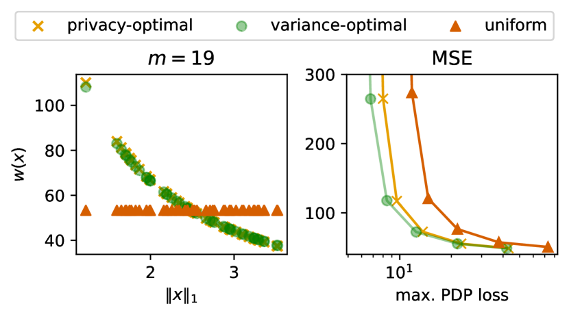
Figure 1: Comparison of sampling strategies for the Laplace sum mechanism. Left: The importance weight for each data point produced. Each dot in the plot represents a single data point. The points are ordered by their $\ell_{1}$-norm. Right: Estimation error for varying noise scales. Lower is better. The horizontal axis is the maximum PDP loss over the data set.

We conclude this section with a simple numerical example for Theorems 3.2 and 3.6 to illustrate that (i) privacy and accuracy are often well-aligned goals in importance sampling and (ii) uniform sampling is highly suboptimal even for very fundamental mechanisms. For this purpose, we generate synthetic data and compare informative importance sampling distributions to uniform sampling in terms of privacy and variance at a fixed expected sample size.

We return to the Laplacian weighted sum mechanism

$$\mathcal{M}_{\text{LWS}}(\widetilde{\mathcal{D}})=\zeta+\sum_{i=1}^{n}w_{i}\mathbf{x}_{i}$$

as an example, where $\widetilde{\mathcal{D}}=\{(w_{i},\mathbf{x}_{i})\}_{i\in\mathcal{I}}$ is a weighted data set and $\zeta$ is standard Laplace distributed. When $\widetilde{\mathcal{D}}$ is obtained by Poisson importance sampling $\mathcal{S}_{q}$ from a data set $\mathcal{D}=\{\mathbf{x}_{i}\}_{i=1}^{n}$, then the mechanism $\mathcal{M}_{\text{LWS}}\circ\mathcal{S}_{q}$ has variance

$$\operatorname{Var}\mathopen{}\mathclose{{}\left[\mathcal{M}_{\text{LWS}}(\widetilde{\mathcal{D}})_{j}}\right]=2+\sum_{i=1}^{n}\mathopen{}\mathclose{{}\left(\frac{1}{q(\mathbf{x}_{i})}-1}\right)\mathbf{x}_{ij}^{2}$$

in the $j$-th dimension. We compare three sampling strategies: uniform sampling $q_{\text{unif}}(\mathbf{x})=m/n$, privacy-optimal sampling $q_{\text{priv}}$ according to Theorem 3.6, and variance-optimal sampling $q_{\text{var}}$, defined as the solution to the following optimization problem:

$$\min_{q}\quad\operatorname{Var}\mathopen{}\mathclose{{}\left[\mathcal{M}_{\text{LWS}}(\widetilde{\mathcal{D}})}\right]\quad\textnormal{subject to}\quad \sum_{i=1}^{n}q(\mathbf{x}_{i})=m.$$

We generate $n=$1000$$ points from an isotropic multivariate normal distribution in $d=10$ dimensions with variance $\sigma^{2}=1/d$ in each dimension.

First, we visualize the importance weights $w(\mathbf{x}_{i})$ for each sampling strategy. For this, we fix a target sample size at $m=19$ and compute the weights $w(\mathbf{x}_{i})$ for each sampling strategy that achieve the target sample size in expectation. The results are shown in Figure 1 (left). Remarkably, the privacy-optimal weights and the variance-optimal weights are almost identical.

Next, we compare mean-squared error (MSE) and privacy loss of the sampling strategies at different privacy levels. For this, we vary the noise scale $b$ of the Laplace mechanism over a coarse grid in $[3,3000]$. For each $b$, we fix the expected sample size $m_{b}$ by computing the privacy-optimal weights. Then, we compute the corresponding weights for the other two sampling strategies such that they achieve $m_{b}$ in expectation. We then compute the individual PDP losses $\psi(\mathbf{x}_{i})$ for each sampling strategy and obtain their respective maximum over the data set. Finally, we compute the MSE of each sampling strategy by averaging over 1000 independent runs. The resulting PDP losses and MSEs are shown in Figure 1 (right).

4 Importance Sampling for DP $k$-means

In this section, we apply our results on privacy amplification for importance sampling to the DP $k$-means problem. We define a weighted version of the DP-Lloyd algorithm, and analyze its PDP profile. Then, we derive the required constants for the privacy-optimal distribution and estabilsh a privacy guarantee for the coreset-based sampling distribution. We provide proofs in Appendix D.

Differentially Private $k$-means Clustering.  Given a data set $\mathcal{D}$ as introduced before, the goal of $k$-means clustering is to find a set of $k\in\mathbb{N}$ cluster centers $\mathcal{C}=\{\mathbf{c}_{1},\ldots,\mathbf{c}_{k}\}$ that minimize the distance of the data points to their closest cluster center. The objective function is given as $\phi_{\mathcal{D}}(\mathcal{C})=\sum_{i=1}^{n}d(\mathbf{x}_{i},\mathcal{C})$, where $d(\cdot,\cdot)$ is the distance of a point $\mathbf{x}$ to its closest cluster center $\mathbf{c}_{j}$, which is $d(\mathbf{x},\mathcal{C})=\min_{j}\|\mathbf{x}-\mathbf{c}_{j}\|^{2}$. The standard approach of solving the $k$-means problem is Lloyd’s algorithm (Lloyd, 1982). It starts by initializing the cluster centers $\mathcal{C}$ and then alternates between two steps. First, given the current cluster centers $\mathcal{C}$, we compute the cluster assignments $\mathcal{C}_{j}=\{\mathbf{x}_{i}\mid j=\operatorname*{arg\,min}_{j}\|\mathbf{x}_{i}-\mathbf{c}_{j}\|^{2}\}$ for every $j=1,\ldots,k$. Second, we update all cluster centers to be the mean of their cluster $\mathbf{c}_{j}=\frac{1}{|\mathcal{C}_{j}|}\sum_{\mathbf{x}\in\mathcal{C}_{j}}\mathbf{x}$. Those two steps are iterated until convergence.

A generic way to make Lloyd’s algorithm differentially private is to add appropriately scaled noise to both steps of the algorithm. This was first suggested by Blum et al. (2005) and later refined by Su et al. (2016, 2017). In this paper, we follow the variant of Su et al. (2016), which we refer to as DP-Lloyd. Let $\xi\in\mathbb{R}^{k}$ be a random vector whose entries independently follow a zero mean Laplace distribution with scale $\beta_{\mathrm{count}}>0$. Furthermore, let $\zeta_{1},\ldots,\zeta_{k}\in\mathbb{R}^{d}$ be random vectors whose entries independently follow a zero mean Laplace distribution with scale $\beta_{\mathrm{sum}}>0$. The update of the cluster centers as well as the number of points per cluster are noisy:

$$\mathbf{c}_{j}=\frac{1}{\xi_{j}+|\mathcal{C}_{j}|}\mathopen{}\mathclose{{}\left(\zeta_{j}+\sum_{\mathbf{x}\in\mathcal{C}_{j}}\mathbf{x}}\right).$$

Assuming the points have bounded $\ell_{1}$-norm, i.e., $\mathcal{X}=\mathcal{B}_{1}(r)$ for some $r>0$, DP-Lloyd preserves $\epsilon$-DP with $\epsilon=\mathopen{}\mathclose{{}\left(r/\beta_{\mathrm{sum}}+1/\beta_{\mathrm{count}}}\right)T$ after $T$ iterations. Su et al. (2016) suggest allocating the noise variance across the two steps as $\beta_{\mathrm{count}}/\beta_{\mathrm{sum}}=\sqrt[3]{4d\rho^{2}}$, where $\rho\approx 0.225$ is an empirically derived constant.

Weighted DP Lloyd’s Algorithm.  In order to apply importance subsampling to $k$-means, we first define a weighted version of DP-Lloyd. Each iteration of DP-Lloyd consists of a counting query and a sum query, which generalize naturally to the weighted scenario. Specifically, for a weighted data set $\mathcal{S}=\{(w_{i},\mathbf{x}_{i})\}_{i=1}^{n}$ we define the update step to be

$$\mathbf{c}_{j}=\frac{1}{\xi_{j}+\sum_{(w,\mathbf{x})\in\mathcal{C}_{j}}w}\mathopen{}\mathclose{{}\left(\zeta_{j}+\sum_{(w,\mathbf{x})\in\mathcal{C}_{j}}w\mathbf{x}}\right).$$

Just as before, $\xi\in\mathbb{R}^{k}$ and $\zeta\in\mathbb{R}^{k\times d}$ each have iid Laplace-distributed entries with scale $\beta_{\mathrm{count}}>0$ and $\beta_{\mathrm{sum}}>0$, respectively. This approach admits a PDP profile that generalizes naturally from the $\epsilon$-DP guarantee without sampling and it is summarized in Algorithm 2 which can be found in Appendix D.

Proposition 4.1.

The weighted DP Lloyd algorithm (Algorithm 2) satisfies the PDP profile

$$\epsilon_{\mathrm{Lloyd}}(w,\mathbf{x})=\mathopen{}\mathclose{{}\left(\frac{1}{\beta_{\mathrm{count}}}+\frac{\|\mathbf{x}\|_{1}}{\beta_{\mathrm{sum}}}}\right)Tw.$$ (3)

Privacy-optimal sampling.  In order to compute the privacy-optimal weights via Algorithm 1, we need the strong convexity constant of $\epsilon_{\mathrm{Lloyd}}$, which is readily obtained via the second derivative:

$$\frac{\partial^{2}}{\partial^{2}w}\exp\mathopen{}\mathclose{{}\left(\epsilon_{\mathrm{Lloyd}}(w,\mathbf{x})}\right)$$

$$\geq T^{2}\mathopen{}\mathclose{{}\left(\frac{1}{\beta_{\mathrm{count}}}+\frac{\|\mathbf{x}\|_{1}}{\beta_{\mathrm{sum}}}}\right)\exp\mathopen{}\mathclose{{}\left(\mathopen{}\mathclose{{}\left(\frac{1}{\beta_{\mathrm{count}}}+\frac{\|\mathbf{x}\|_{1}}{\beta_{\mathrm{sum}}}}\right)T}\right)$$ (4)

$$=\colon\mu.$$

Besides the privacy-optimal distribution, we also consider a coreset-based sampling distribution. Before doing so, we first introduce the idea of a coreset.

Coresets for $k$-means.  A coreset is a weighted subset $\mathcal{S}\subseteq\mathcal{D}$ of the full data set $\mathcal{D}$ with cardinality $m\ll n$, on which a model performs provably competitive when compared to the performance of the model on $\mathcal{D}$. Since we are now dealing with weighted data sets, we define the weighted objective of $k$-means to be $\phi_{\mathcal{D}}(\mathcal{C})=\sum_{\mathbf{x}\in\mathcal{D}}w(\mathbf{x})d(\mathbf{x},\mathcal{C})$, where $w(\mathbf{x})\geq 0$ are the non-negative weights. In this paper, we use a sampling distribution inspired by a lightweight-coreset construction as introduced by Bachem et al. (2018).

Definition 4.2 (Lightweight coreset).

Let $\varepsilon>0$, $k\in\mathbb{N}$, and $\mathcal{D}\subseteq\mathcal{X}$ be a set of points with mean $\bar{\mathbf{x}}$. A weighted set $\mathcal{S}$ is a $(\varepsilon,k)$-lightweight-coreset of the data $\mathcal{D}$ if for any $\mathcal{C}\subseteq\mathbb{R}^{d}$ of cardinality at most $k$ we have $|\phi_{\mathcal{D}}(\mathcal{C})-\phi_{\mathcal{S}}(\mathcal{C})|\leq\frac{\varepsilon}{2}\phi_{\mathcal{D}}(\mathcal{C})+\frac{\varepsilon}{2}\phi_{\mathcal{D}}(\{\bar{\mathbf{x}}\})$.

Note that the definition holds for any choice of cluster centers $\mathcal{C}$. Bachem et al. (2018) propose the sampling distribution $q(\mathbf{x})=\frac{1}{2}\frac{1}{n}+\frac{1}{2}\frac{d(\mathbf{x},\bar{\mathbf{x}})}{\sum_{i=1}^{n}d(\mathbf{x}_{i},\bar{\mathbf{x}})}$ and assign each sampled point $\mathbf{x}$ the weight $(mq(\mathbf{x}))^{-1}$. This is a mixture distribution of a uniform and a data-dependent part. Note that by using these weights, $\phi_{\mathcal{S}}(\mathcal{C})$ yields an unbiased estimator of $\phi_{\mathcal{D}}(\mathcal{C})$. The following theorem shows that this sampling distribution yields a lightweight-coreset with high probability.

Theorem 4.3 (Bachem et al. (2018)).

Let $\varepsilon>0,\Delta\in(0,1)$, $k\in\mathbb{N}$, $\mathcal{D}$ be a set of points in $\mathcal{X}$, and $\mathcal{S}$ be the sampled subset according to $q$ with a sample size $m$ of at least $m\geq c\frac{kd\log k-\log\Delta}{\varepsilon^{2}}$, where $c>0$ is a constant. Then, with probability of at least $1-\Delta$, $\mathcal{S}$ is an $(\varepsilon,k)$-lightweight-coreset of $\mathcal{D}$.

Coreset-based sampling distribution.  We adapt the sampling distribution used in Theorem 4.3 slightly and propose $q(\mathbf{x})=\lambda\frac{m}{n}+(1-\lambda)\frac{m\|\mathbf{x}\|_{1}}{n\tilde{\mathbf{x}}}$, where $m\ll n$ is the expected subsample size and $\tilde{\mathbf{x}}=\frac{1}{n}\sum_{i=1}^{n}\|\mathbf{x}\|_{1}$ is the average $\ell_{1}$-norm. There are three changes: (i) we assume the data set $\mathcal{X}$ is centered, (ii) we introduce $\lambda\in[0,1]$ which yields a uniform sampler for the choice of $\lambda=1$, and (iii) we change the distance from $\|\cdot\|_{2}^{2}$ to $\|\cdot\|_{1}$ because the privacy of the Laplace mechanism is based on the $\ell_{1}$-norm. With this distribution, we have the following $\epsilon$-DP guarantee.

Proposition 4.4.

Let $\mathcal{X}=\mathcal{B}_{1}(r)$ for some $r>0$, $\mathcal{D}=\{\mathbf{x}_{i}\}_{i=1}^{n}\subseteq\mathcal{X}$ be a centered data set with $\sum_{i=1}^{n}\mathbf{x}_{i}=0$, and suppose $\tilde{\mathbf{x}}=\frac{1}{n}\sum_{i=1}^{n}\|\mathbf{x}\|_{1}$ is known. For any $\lambda\in[0,1]$ and $m\leq n{\tilde{\mathbf{x}}}/{r}$, let $q(\mathbf{x})=\lambda\frac{m}{n}+(1-\lambda)\frac{m\|\mathbf{x}\|_{1}}{n\tilde{\mathbf{x}}}$. Furthermore, let $\mathcal{M}(\cdot)$ be Algorithm 2. Then, $\mathbb{E}[|S_{q}(\mathcal{D})|]=m$ and $\mathcal{M}(S_{q}(\mathcal{D}))$ satisfies $\epsilon$-DP with

$$\epsilon=\log\mathopen{}\mathclose{{}\left(1+\max\mathopen{}\mathclose{{}\left\{\vartheta(A_{1},A_{2}),\ \vartheta(A_{1}^{\prime},A_{2}^{\prime})}\right\}}\right),$$ (5)

where $A_{1}=\mathopen{}\mathclose{{}\left(1/\beta_{\mathrm{count}}+r/\beta_{\mathrm{sum}}}\right)T$, $A_{1}^{\prime}=T/\beta_{\mathrm{count}}$, $A_{2}=m/n\mathopen{}\mathclose{{}\left(\lambda+(1-\lambda)r/\tilde{\mathbf{x}}}\right)$, $A_{2}^{\prime}=\lambda m/n$, and $\vartheta(u,v)=\mathopen{}\mathclose{{}\left(e^{u/v}-1}\right)v$.

Note that $A_{1}$ is simply the differential privacy guarantee of the standard DP-Lloyd algorithm without sampling and $A_{2}=\max_{\mathbf{x}\in\mathcal{X}}\,q(\mathbf{x})\leq 1$. The $\max$ in Equation (5) arises because the PDP profile $\psi(\mathbf{x})$ is not necessarily monotonic in $\mathbf{x}$, but is always maximized at the boundary of the domain, i.e., at $\|\mathbf{x}\|_{1}\in\{0,r\}$.

5 Experiments

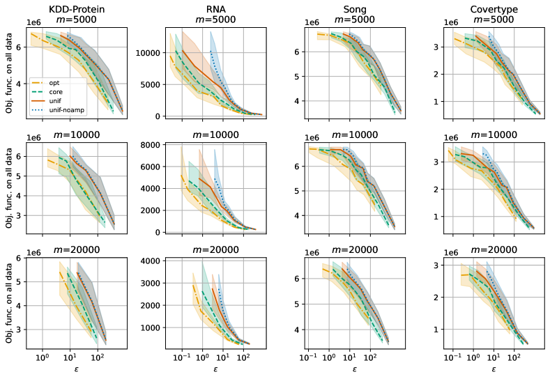
Figure 2: Cost-$\epsilon$-loss ratios on KDD-Protein, RNA, Song, and Covertype data.

We now evaluate our proposed sampling approaches (coreset-based and privacy-optimal) on the task of $k$-means clustering and we are interested in three objectives: privacy, efficiency, and accuracy. The point of the experiments is to investigate whether our proposed sampling strategies lead to improvements in terms of the three objectives when compared to uniform sampling. Our measure for efficiency is the subsample size $m$ produced by the sampling strategy. This is because Lloyd’s algorithm scales linearly in $m$ (for fixed $k$ and $T$) and the computing time of the sampling itself is negligible in comparison. We measure accuracy via the $k$-Means objective evaluated on the full data set and privacy as the $\epsilon$-DP guarantee of the sampled mechanism.

Data.  We use the following seven real-world data sets: Ijcnn1 (Chang & Lin, 2001) ($n=49,990$, $d=22$), Pose (Catalin Ionescu, 2011; Ionescu et al., 2014) ($n=35,832$, $d=48$), MiniBooNE (Dua & Graff, 2017) ($n=130,064$, $d=50$), KDD-Protein ($n=145,751$, $d=74$), RNA (Uzilov et al., 2006) ($n=488,565$, $d=8$), Song (Bertin-Mahieux et al., 2011) ($n=515,345$, $d=90$), and Covertype (Blackard & Dean, 1999) ($n=581,012$, $d=54$).

We pre-process the data sets to ensure each data point has bounded $\ell_{1}$-norm. Following the common approach in differential privacy to bound contributions at a quantile (Abadi et al., 2016; Geyer et al., 2017; Amin et al., 2019), we set the $\ell_{1}$ cut-off point $r$ to the 97.5 percentile and discard the points whose norm exceeds $r$. Moreover, we center each data set since this is a prerequisite for the coreset-based sampling distribution. We discuss possible limitations of this in Section 6.

Setup.  The specific task we consider is $k$-means for which we use the weighted version of DP-Lloyd. We fix the number of iterations of DP-Lloyd to $T=10$ and the number of clusters to $k=25$. The scale parameters are set to $\beta_{\mathrm{sum}}=\sqrt{\frac{Tr}{B}}\sqrt[3]{\frac{d}{2\rho}}$ and $\beta_{\mathrm{count}}=\sqrt[3]{4d\rho^{2}}\beta_{\mathrm{sum}}$, where $\rho=0.225$ and $B$ is a constant we vary between $B\in\{0.0001,0.001,0.01\}$ in order to compare performance at different privacy levels.

We evaluate the following three different importance samplers and use various sample sizes, i.e., $m\in\{5000,10000,20000\}$. For the coreset-based (core) sampling, the sampling distribution is $q_{\text{core}}(\mathbf{x})=\lambda\frac{m}{n}+(1-\lambda)\frac{m\|\mathbf{x}\|_{1}}{n\tilde{\mathbf{x}}}$, where we set $\lambda=\frac{1}{2}$. The privacy guarantee is computed via Proposition 4.4. The uniform (unif) sampling uses $q_{\text{unif}}(\mathbf{x})=m/n$ and we compute the privacy guarantee via Proposition 4.4. Note that it is the same $q$ as in core but with $\lambda=1$. For the privacy-optimal (opt) sampling, we compute $q_{\text{priv}}(\mathbf{x})$ numerically via Algorithm 1 for the target $\epsilon^{\star}=\mathopen{}\mathclose{{}\left(r/\beta_{\mathrm{sum}}+1/\beta_{\mathrm{count}}}\right)T$ using the strong convexity constant from Equation (4). For reference, we also include the performance of uniform sampling when amplification is not accounted for (unif-noamp).

Due to the stochasticity in the subsampling process and the noises within DP-Lloyd, we repeat each experiment 50 times with different seeds and report on median performances. In addition, we depict the 75% and 25% quartiles. Note that the weighted version of DP-Lloyd is only used when learning the cluster centers. For the sampling-based approaches, we re-compute the objective function (cost) on all data after optimization and report on the total cost scaled by the number of data points $n^{-1}$. The code is implemented in Python using numpy (Harris et al., 2020). All experiments run on an Intel Xeon machine with 28 cores with 2.60 GHz and 256 GB of memory.

Results.  Figure 2 depicts the results for KDD-Protein, RNA, Song, and Covertype. Within the figure, each column corresponds to a data set and the rows show different subsampling sizes $m$. The curves are obtained by varying $B$ and show the cost of $k$-means evaluated on all data as a function of the privacy loss $\epsilon$. Note that the $x$-axis is in log-scale, shared column-wise, and that the optimal location is the bottom left since it yields a low cost and a low privacy loss. Additional results on Ijcnn1, Pose, and MiniBooNE are shown in Figure 3 in Appendix B.

The performance of a uniform subsample of the data set of size $m$ with no privacy amplification is depicted as unif-noamp (blue line) and generally yields the worst results. Privacy amplification using a uniform subsampling strategy (unif, red line) performs similar in terms of cost but improves the privacy especially in low $\epsilon$ cases. Our proposed subsampling strategy core (green line) consistently outperforms unif as it yields a better cost-$\epsilon$-loss ratio. The opt (orange line) sampler often further improves upon core or performs on-par. Furthermore, we evaluate the cost as a function of the subsample size $m$ for a fix privacy budget $\epsilon$ in Appendix C.

As for the efficiency, the relative runtime matches the fraction of data used for the computation. For example, on KDD-Protein data, using subsets of 5k, 10k, and 20k data points corresponding to 3.5%, 7.0%, and 14.1% of the full data set, respectively, takes approx. 3.2%, 7.0%, and 13.4% of the computation time of DP-Lloyd on the full data set, respectively. Here, the construction time for the sampling distribution is negligible. We consistently observe these findings on the remaining data sets.

6 Discussion & Limitations

Ideally, our coreset-based sampling distribution would have use the squared $\ell_{2}$-norm instead of the $\ell_{1}$-norm in order to align with the theoretical guarantees from Theorem 4.3. The norm change was necessary since the Laplace noise scales with the $\ell_{1}$-norm, not the $\ell_{2}$-norm. Future work could address this by considering $\ell_{2}$-based noise distributions such as Hardt & Talwar (2010) use in Lloyd’s algorithm for $\epsilon$-DP. Despite the absence of a formal utility guarantee, the experiments have demonstrated that the $\ell_{1}$-norm is a suitable heuristic in this regard. Another limitation of the coreset-based approach is that it requires some data set statistics to be known exactly. We accomplished this by computing the data set mean and the average $\ell_{1}$-norm at the pre-processing stage. Strictly speaking, this additional privacy loss should be accounted for. Future work could investigate whether an equivalent utility guarantee could be obtained with approximate knowledge of these statistics. Note also that these limitations only apply to the coreset-based sampling distribution, not to the privacy-optimal distribution.

7 Related Work

The notion of personalized differential privacy is introduced by Jorgensen et al. (2015) and Ebadi et al. (2015), as well as by Alaggan et al. (2016) under the name of heterogeneous differential privacy. In Jorgensen et al. (2015), the privacy parameter is associated with a user, while it is associated with the value of a data point in the work of Ebadi et al. (2015) and ours. Jorgensen et al. (2015) achieve personalized DP by subsampling the data with heterogeneous probabilities, but without accounting for the bias introduced by the heterogeneity. Moreover, this privacy analysis is loose as it does not exploit the inherent heterogeneity of the original mechanism’s privacy guarantee.

Recently, there has been renewed interest in PDP due to its connection to individual privacy accounting and fully adaptive composition (Feldman & Zrnic, 2021; Koskela et al., 2022; Yu et al., 2023). In this context, privacy filters have been proposed as a means to answer more queries about a data set by reducing a PDP guarantee to its worst-case counterpart. Analogously, our privacy-optimal importance sampling distribution can be used to subsample a data set by reducing a PDP guarantee to its worst-case counterpart.

The idea of using importance sampling for differential privacy is not entirely new. Wei et al. (2022) propose a differentially private importance sampler for the mini-batch selection in differentially private stochastic gradient descent. Their sampling distribution resembles the variance-optimal distribution we display in Figure 1. The major drawback of this distribution is its intractability—it requires us to know the quantity we want to compute in the first place. Note that our privacy-optimal distribution is very close to the variance-optimal distribution while being efficient to compute. Moreover, their privacy analysis is restricted to the Gaussian mechanism and does not generalize to general DP or Rényi-DP mechanisms, because it is based on Mironov et al. (2019)’s analysis of the subsampled Gaussian mechanism.

The first differentially private version of $k$-means is introduced by Blum et al. (2005). They propose the Sub-Linear Queries (SuLQ) framework, which, for $k$-means, uses a noisy (Gaussian) estimate of the number of points per cluster and a noisy sum of distances. This is also reported by Su et al. (2016, 2017) which extend the analysis. Other variants of differentially private $k$-means were proposed, e.g., by Balcan et al. (2017); Huang & Liu (2018); Stemmer & Kaplan (2018); Shechner et al. (2020); Ghazi et al. (2020); Nguyen et al. (2021); Cohen-Addad et al. (2022).

Coresets are compact summaries of data sets on which learned models perform provably competitive. Feldman et al. (2007) propose a weak coreset construction for $k$-means clustering that samples points according to their squared distance to the preliminary solution of an approximation. Chen (2009) propose a similar idea. Langberg & Schulman (2010) introduce the notion of sensitivity which measures the importance of a point for preserving the cost over all possible solutions.

8 Conclusion

We analyzed importance sampling in the context of privacy amplification. We then presented a general amplification result for arbitrary PDP mechanisms as well as two distinct applications of this result: (i) deriving the sampling distribution that optimizes the privacy-efficiency trade-off; and (ii) a establishing a $\epsilon$-DP guarantee for a sampling distribution based on coresets. Finally, we evaluated both distributions for DP $k$-means clustering where both outperformed uniform sampling in terms of the privacy-accuracy-efficiency trade-off.

Promising directions for future work include extensions to $(\epsilon,\delta)$-DP or Rényi-DP as well as establishing formal utility guarantees via coresets. Moreover, the privacy-optimal distribution is directly applicable to a streaming setting, which provides an opportunity to improve efficiency further. Additionally, its connection to fairness could be explored where importance sampling is sometimes used to mitigate bias.

Broader impact

We see privacy preservation as an important contributor to making the training of machine learning models beneficial for the general public. This paper contributes methods that improve the practicality and efficiency of privacy-preserving machine learning and could hence accelerate its wider adoption.

Appendix

• Section A discusses the question of “When does sampling improve privacy?”.

• Section B includes experimental results on additional data sets.

• Section C provides empirical results on the accuracy for a fixed privacy budget $\epsilon$.

• Section D contains the proofs for Theorem 3.2, Proposition A.1, Proposition A.2, Theorem 3.2, Proposition 3.8, Proposition 4.1, and finally Proposition 4.4. Moreover, Algorithm 2 describes the weighted version of DP Lloyd.

Appendix A Can sampling improve privacy?

We have pointed out in Sections 1 and 3 that any privacy improvement due to uniform subsampling is typically canceled out by re-weighting the samples. In this section, we make this statement more precise and provide formal conditions on the PDP profile under which weighted sampling does or does not improve privacy when re-weighting is accounted for.

Trivially, any mechanism $\mathcal{M}$ that simply ignores the weights $\{w_{i}\}_{i=1}^{n}$ has a weighted PDP profile $\epsilon(w,\mathbf{x})$ that is constant in $w$. In this case, Theorem 3.2 reduces to the established amplification by subsampling result (Proposition 2.3), which indeed implies that $\widehat{\mathcal{M}}$ satisfies a stronger privacy guarantee than $\mathcal{M}$. The following proposition provides a more general condition under which $\widehat{\mathcal{M}}$ satisfies a stronger privacy guarantee than $\mathcal{M}$.

Proposition A.1.

Let $\mathcal{M}:\mathcal{X}\times[1,\infty)\to\mathcal{Y}$ be an $\epsilon$-PDP mechanism, $\widetilde{\mathcal{M}}$ be its unweighted counterpart defined as $\widetilde{\mathcal{M}}(\{\mathbf{x}_{i}\}_{i=1}^{n})=\mathcal{M}(\{(1,\ \mathbf{x}_{i})\}_{i=1}^{n})$, and $\tilde{\epsilon}(\mathbf{x})=\epsilon(1,\mathbf{x})$ be the PDP profile of $\widetilde{\mathcal{M}}$. Furthermore, let $\epsilon$ be differentiable in $w$ and $\epsilon^{\prime}(w,\mathbf{x})=\partial\epsilon(w,\mathbf{x})/\partial w$. Then, there is a Poisson importance sampler $S(\cdot)$ for which the following holds. Let $\psi$ be the PDP profile of $\mathcal{M}\circ S$ implied by Theorem 3.2. For any $\mathbf{x}\in\mathcal{X}$, if $\epsilon^{\prime}(1,\mathbf{x})<1-e^{-\epsilon(1,\mathbf{x})}$, then $\psi(\mathbf{x})<\tilde{\epsilon}(\mathbf{x})$.

Consequently, if the condition $\epsilon^{\prime}(1,\mathbf{x})<1-e^{-\epsilon(1,\mathbf{x})}$ holds in a neighborhood around the maximizer $\mathbf{x}^{\star}=\operatorname*{arg\,max}_{\mathbf{x}\in\mathcal{X}}\tilde{\epsilon}(\mathbf{x})$, then $\widehat{\mathcal{M}}$ satisfies DP with a strictly smaller privacy parameter than $\mathcal{M}$. However, for the following important class of mechanisms, $\widehat{\mathcal{M}}$ cannot satisfy a stronger privacy guarantee than $\mathcal{M}$.

Proposition A.2.

Let $\mathcal{M}$, $\widetilde{\mathcal{M}}$, $\epsilon$, $\epsilon^{\prime}$, and $\tilde{\epsilon}$ be as in Proposition A.1, $S(\cdot)$ be any Poisson importance sampler, $\psi$ be the PDP profile of $\mathcal{M}\circ S$ implied by Theorem 3.2, and $\mathbf{x}\in\mathcal{X}$. If $\epsilon(w,\mathbf{x})\leq w\epsilon^{\prime}(w,\mathbf{x})$ for all $w\geq 1$, then $\psi(\mathbf{x})\geq\tilde{\epsilon}(\mathbf{x})$.

For instance, the condition $\epsilon(w,\mathbf{x})\leq w\epsilon^{\prime}(w,\mathbf{x})$ is satisfied everywhere by any profile of the form $\epsilon(w,\mathbf{x})=f(\mathbf{x})w^{p}$, where $p\geq 1$ and $f$ is any non-negative function that does not depend on $w$. This includes the Laplacian weighted sum mechanism discussed above, as well as the weighted DP-Lloyd mechanism which we discuss in Section 4.

It is important to note that, even in a case where we cannot hope to improve upon the original mechanism, it is still possible to obtain a stronger privacy amplification than with uniform subsampling at the same sampling rate. Indeed, the uniform distribution is never optimal unless the PDP profile of the original mechanism is constant.

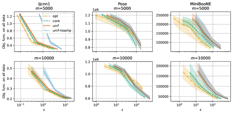
Figure 3: Cost-$\epsilon$-loss ratios on Ijcnn1, Pose, and MiniBooNE data.

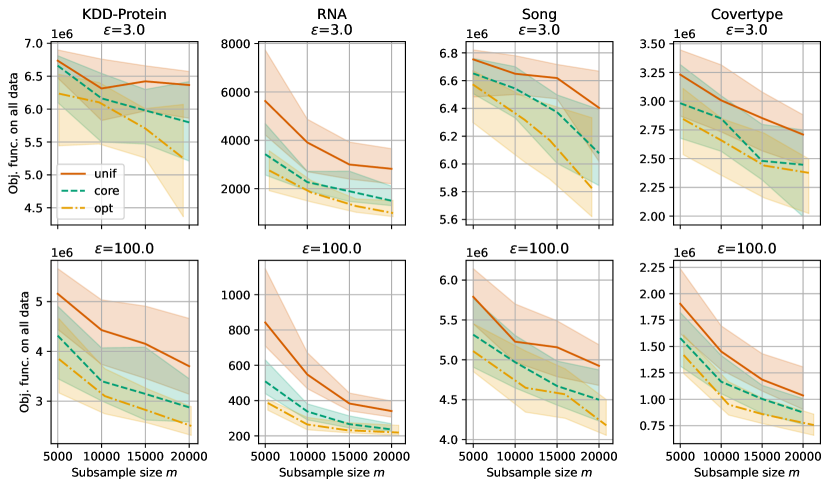
Figure 4: Cost-sample-size-$m$ ratios on KDD-Protein, RNA, Song, and Covertype data.

Figure 5: Cost-sample-size-$m$ ratios on Ijcnn1, Pose, and MiniBooNE data.

Appendix B Results on the Remaining Data Sets

Figure 3 depicts the results for the remaining data sets Ijcnn1, Pose, and MiniBooNE. Note that those data sets are slightly smaller in terms of the number of data points as the data sets shown in Figure 2, thus, we drop the $m=$20000$$ scenario. On Ijcnn1, there is a substantial privacy gain when compared to unif-noamp, where we do not account for privacy amplification. On Pose data, it appears that one choice of $B$ yields a worse result for the privacy-optimal sampling than for coreset-based sampling. This can happen because the privacy-optimal sampling strategy only optimizes two out of three objectives: privacy and efficiency but not accuracy. Although privacy and accuracy are often well aligned in this problem, there is no formal guarantee on the accuracy. In particular, the degree of alignment between privacy and accuracy depends on the specific mechanism and data set used. The performance on MiniBooNE is consistent with the performances of the data sets in Figure 2.

Appendix C Accuracy Results for a Fixed $\epsilon$

We now take a closer look on the performance of the subsampling strategies as a function of the subsample size $m$. For this scenario, we fix the privacy budget to either $\epsilon=3$ or $\epsilon=100$. Figure 4 depicts the results for the data sets KDD-Protein, RNA, Song, and Covertype while Figure 5 shows the results on Ijcnn1, Pose, and MiniBooNE data. As expected, the total cost decreases as we increase the subsample size $m$. Moreover, we can see that unif (red line) almost consistently performs worst while the coreset-inspired sampling core (green line) yields lower total cost for the same $m$ and $\epsilon$. The exception is on Ijcnn1 for the $\epsilon=100$ case where all methods perform alike. As in the previous experiment, the sampler using the privacy-optimal weights opt (orange line) further improves upon the performance of core by yielding even lower costs.

Appendix D Proofs

This section contains the proofs of all our theoretical results. For completeness, we do not only restate the theorems and propositions, but also the used algorithms, assumptions, and problems.

D.1 Theorem 3.2

See 3.2

Proof.

The proof is analogous to the proof of the regular privacy amplification theorem with $\delta=0$, see, e.g., Steinke (2022, Theorem 29). Let $\mathcal{A}$ be any measurable subset from the probability space of $\mathcal{M}(\mathcal{D})$. We begin by defining the functions $P(\mathcal{Z})=\Pr\mathopen{}\mathclose{{}\left[\widehat{\mathcal{M}}(\mathcal{D})\in\mathcal{A}\mid S_{q}(\mathcal{D})=\mathcal{Z}}\right]$ and $P^{\prime}(\mathcal{Z})=\Pr\mathopen{}\mathclose{{}\left[\widehat{\mathcal{M}}(\mathcal{D}^{\prime})\in\mathcal{A}\mid S_{q}(\mathcal{D}^{\prime})=\mathcal{Z}}\right]$. Let $\mathcal{D}=\mathcal{D}^{\prime}\cup\{\mathbf{x}\}$ for some $\mathbf{x}\in\mathcal{X}$. Note that

$$\begin{split}\Pr\mathopen{}\mathclose{{}\left[\widehat{\mathcal{M}}(\mathcal{D})\in\mathcal{A}}\right]&=\mathbb{E}\mathopen{}\mathclose{{}\left[P(S_{q}(\mathcal{D}))}\right]\\ &=(1-q(\mathbf{x}))\mathbb{E}\mathopen{}\mathclose{{}\left[P(S_{q}(\mathcal{D}))\mid\mathbf{x}\in S_{q}(\mathcal{D})}\right]+q(\mathbf{x})\mathbb{E}\mathopen{}\mathclose{{}\left[P(S_{q}(\mathcal{D}))\mid\mathbf{x}\notin S_{q}(\mathcal{D})}\right].\end{split}$$ (6)

We can analyze the events $\mathbf{x}\in S_{q}(\mathcal{D})$ and $\mathbf{x}\notin S_{q}(\mathcal{D})$ separately as follows. Conditioned on the event $\mathbf{x}\notin S_{q}(\mathcal{D})$, the distributions of $S_{q}(\mathcal{D})$ and $S_{q}(\mathcal{D}^{\prime})$ are identical since all selection events $\gamma_{i}$ are independent:

$$\mathbb{E}\mathopen{}\mathclose{{}\left[P(S_{q}(\mathcal{D}))\mid\mathbf{x}\notin S_{q}(\mathcal{D})}\right]=\mathbb{E}\mathopen{}\mathclose{{}\left[P(S_{q}(\mathcal{D}^{\prime}))\mid\mathbf{x}\notin S_{q}(\mathcal{D})}\right]=\mathbb{E}\mathopen{}\mathclose{{}\left[P^{\prime}(S_{q}(\mathcal{D}^{\prime}))}\right].$$ (7)

On the other hand, conditioned on the event $\mathbf{x}\in S_{q}(\mathcal{D})$, the sets $S_{q}(\mathcal{D})$ and $S_{q}(\mathcal{D})\setminus\{\mathbf{x}\}$ are neighboring, and the distributions of $S_{q}(\mathcal{D})\setminus\{\mathbf{x}\}$ and $S_{q}(\mathcal{D}^{\prime})$ are identical. We can use the PDP profile $\epsilon$ to bound

$$\begin{split}\mathbb{E}\mathopen{}\mathclose{{}\left[P(S_{q}(\mathcal{D}))\mid\mathbf{x}\in S_{q}(\mathcal{D})}\right]&\leq\mathbb{E}\mathopen{}\mathclose{{}\left[e^{\epsilon(1/q(\mathbf{x}),\mathbf{x})}P^{\prime}(S_{q}(\mathcal{D}^{\prime}))\mid\mathbf{x}\in S_{q}(\mathcal{D})}\right]\\ &=e^{\epsilon(1/q(\mathbf{x}),\mathbf{x})}\mathbb{E}\mathopen{}\mathclose{{}\left[P^{\prime}(S_{q}(\mathcal{D}^{\prime}))}\right].\end{split}$$ (8)

Plugging Equations (7) and (LABEL:eq:positive-case) into Equation (LABEL:eq:conditional-expectations) yields

$$\Pr\mathopen{}\mathclose{{}\left[\widehat{\mathcal{M}}(\mathcal{D})\in\mathcal{A}}\right] \leq(1-q(\mathbf{x}))\mathbb{E}\mathopen{}\mathclose{{}\left[P^{\prime}(S_{q}(\mathcal{D}^{\prime}))}\right]+q(\mathbf{x})e^{\epsilon(1/q(\mathbf{x}),\mathbf{x})}\mathbb{E}\mathopen{}\mathclose{{}\left[P^{\prime}(S_{q}(\mathcal{D}^{\prime}))}\right]$$

$$=\mathopen{}\mathclose{{}\left(1+q(\mathbf{x})\mathopen{}\mathclose{{}\left(e^{1/q(\mathbf{x})}-1}\right)}\right)\mathbb{E}\mathopen{}\mathclose{{}\left[P^{\prime}(S_{q}(\mathcal{D}^{\prime}))}\right]$$

$$=\mathopen{}\mathclose{{}\left(1+q(\mathbf{x})\mathopen{}\mathclose{{}\left(e^{1/q(\mathbf{x})}-1}\right)}\right)\Pr\mathopen{}\mathclose{{}\left[\widehat{\mathcal{M}}(\mathcal{D}^{\prime})\in\mathcal{A}}\right].$$

An identical argument shows that

$$\Pr\mathopen{}\mathclose{{}\left[\widehat{\mathcal{M}}(\mathcal{D})\in\mathcal{A}}\right] \geq\frac{1}{1+q(\mathbf{x})\mathopen{}\mathclose{{}\left(e^{1/q(\mathbf{x})}-1}\right)}\Pr\mathopen{}\mathclose{{}\left[\widehat{\mathcal{M}}(\mathcal{D}^{\prime})\in\mathcal{A}}\right].$$

∎

D.2 Proposition A.1

See A.1

Proof.

Let $\mathbf{x}\in\mathcal{X}$ be any data point for which $\epsilon^{\prime}(1,\mathbf{x})<1-e^{-\epsilon(1,\mathbf{x})}$ holds. The core idea of the proof is to treat $\psi(\mathbf{x})$ as a function of the selection probability $q(\mathbf{x})$ and show that it is increasing at $q(\mathbf{x})=1$. We write $\psi_{q(\mathbf{x})}(\mathbf{x})$ to make the dependence on $q(\mathbf{x})$ explicit and define $\omega(w)=\exp(\psi_{1/w}(\mathbf{x}))-1$. We have

$$\frac{\mathrm{d}\omega(1)}{\mathrm{d}w} =e^{\epsilon(1,\mathbf{x})}\mathopen{}\mathclose{{}\left(\epsilon^{\prime}(1,\mathbf{x})-1}\right)+1$$

$$<e^{\epsilon(1,\mathbf{x})}\mathopen{}\mathclose{{}\left(\mathopen{}\mathclose{{}\left(1-e^{-\epsilon(1,\mathbf{x})}}\right)-1}\right)+1$$

$$=0,$$

and, hence, $\mathrm{d}\psi_{q(\mathbf{x})}(\mathbf{x})/\mathrm{d}q(\mathbf{x})>0$ at $q(\mathbf{x})=1$. As a result, there is a probability $q(\mathbf{x})<1$ such that $\psi_{q(\mathbf{x})}(\mathbf{x})<\psi_{1}(\mathbf{x})=\tilde{\epsilon}(\mathbf{x})$. ∎

D.3 Proposition A.2

See A.2

Proof.

As in Proposition A.1, the core idea is to treat $\psi(\mathbf{x})$ as a function of the selection probability $q(\mathbf{x})$. We show that $\psi(\mathbf{x})$ is non-increasing in $q(\mathbf{x})$ if the condition $\epsilon(w,\mathbf{x})\leq w\epsilon^{\prime}(w,\mathbf{x})$ is satisfied for all $w$.

Let $q(\mathbf{x})$ be the selection probability of $\mathbf{x}$ under $S$. We write $\psi_{q}(\mathbf{x})$ to make the dependence on $q(\mathbf{x})$ explicit. Let $\mathbf{x}\in\mathcal{X}$ be arbitrary but fixed and define $\omega(w)=\exp(\psi_{1/w}(\mathbf{x}))-1$. We have

$$\frac{\mathrm{d}\omega(w)}{\mathrm{d}w} =\frac{e^{\epsilon(w,\mathbf{x})}\mathopen{}\mathclose{{}\left(w\epsilon^{\prime}(w,\mathbf{x})-1}\right)+1}{w^{2}}$$

$$\geq\frac{e^{\epsilon(w,\mathbf{x})}\mathopen{}\mathclose{{}\left(\epsilon(w,\mathbf{x})-1}\right)+1}{w^{2}}$$

$$\geq\frac{\mathopen{}\mathclose{{}\left(\epsilon(w,\mathbf{x})+1}\right)\mathopen{}\mathclose{{}\left(\epsilon(w,\mathbf{x})-1}\right)+1}{w^{2}}$$

$$\geq\frac{\epsilon(w,\mathbf{x})^{2}}{w^{2}}$$

$$\geq 0,$$

where we used the assumption $\epsilon(w,\mathbf{x})\leq w\epsilon^{\prime}(w,\mathbf{x})$ in the first inequality and the fact that $e^{z}\geq z+1$ for all $z\geq 0$ in the second inequality. As a result, $\omega$ is minimized at $w=1$ and, hence, $\psi_{q}$ is minimized at $q(\mathbf{x})=1$. To complete the proof, observe that $\psi_{q}(\mathbf{x})=\tilde{\epsilon}(\mathbf{x})$ for $q(\mathbf{x})=1$. ∎

D.4 Theorem 3.6

See 3.3

See 3.4 See 3.5 See 3.7

See 1

See 3.6

Proof.

Since the objective is additive over $w_{i}$ and each constraint only affects one $w_{i}$, we can consider each $w_{i}$ separately. An equivalent formulation of the problem is

$$\max_{w_{i}}\quad w_{i}$$

subject to $$\log\mathopen{}\mathclose{{}\left(1+\frac{1}{w_{i}}\mathopen{}\mathclose{{}\left(e^{\epsilon(w_{i},\mathbf{x}_{i})}-1}\right)}\right)\leq\epsilon^{\star}$$

$$w_{i}\geq 1.$$

Assumption 3.4 guarantees that the feasible region is bounded and Assumption 3.5 guarantees that it is non-empty. Since the objective is strictly monotonic, the solution must be unique. ∎

D.5 Proposition 3.8

See 3.8

Before beginning the proof, we state the definition of strong convexity for completeness.

Definition D.1 (Strong convexity).

Let $\mu>0$. A differentiable function $f:\mathbb{R}^{d}\to\mathbb{R}$ is $\mu$-strongly convex if

$$f(v)\geq f(u)+\nabla f(u)^{\mkern-1.5mu\mathsf{T}}(v-u)+\frac{\mu}{2}\|v-u\|_{2}^{2}\qquad\text{for all $u,v\in\mathbb{R}^{d}$}.$$ (9)

Proof of Proposition 3.8.

First, we show that Assumption 3.7 implies Assumption 3.5. That is, we want to find a value $v_{i}$ for each $i$ such that all $w_{i}\geq v_{i}$ are infeasible. For some fixed $i$, define $g(w)=\epsilon(w,\mathbf{x}_{i})$ and $g^{\prime}(w)=\frac{\mathrm{d}}{\mathrm{d}w}g(w)$. We apply the strong convexity condition from Equation (9) to $\exp\circ\,g$ at $u=1$ and $v=w$:

$$e^{g(w)} \geq e^{g(1)}+g^{\prime}(1)e^{g(1)}(w-1)+\frac{\mu_{i}}{2}\|w-1\|_{2}^{2}$$

$$\frac{1}{w}\mathopen{}\mathclose{{}\left(e^{g(w)}-1}\right) \geq\frac{\mu}{2}w+\mathopen{}\mathclose{{}\left(e^{g(1)}-g^{\prime}(1)e^{g(1)}+\frac{\mu}{2}-1}\right)\frac{1}{w}+g^{\prime}(1)e^{g(1)}-\mu$$

$$\frac{1}{w}\mathopen{}\mathclose{{}\left(e^{g(w)}-1}\right) \geq b_{1}w^{1}+b_{0}w^{0}+b_{-1}w^{-1}$$

for appropriately defined constants $b_{1}$, $b_{0}$, and $b_{-1}$. We need to distinguish two cases, based on the sign of $b_{-1}$.

Case 1: $b_{-1}<0$.  In this case, we have $b_{-1}w^{-1}\geq b_{-1}$ for all $w\geq 1$. A sufficient condition for infeasibility is

$$b_{1}w+b_{0}+b_{-1} \geq e^{\epsilon^{\star}}-1$$

$$w \geq\frac{e^{\epsilon^{\star}}-1-b_{0}-b_{-1}}{b_{1}}$$

$$w \geq\frac{e^{\epsilon^{\star}}-e^{g(1)}+\mu/2}{\mu/2}$$

$$w \geq 2\mathopen{}\mathclose{{}\left(\frac{e^{\epsilon^{\star}}-e^{g(1)}-\mu/2}{\mu}+1}\right).$$

Case 2: $b_{-1}\geq 0$.  In this case, we have $b_{-1}w^{-1}\geq 0$. Analogously to Case 1, the condition for infeasibility is

$$b_{1}w+b_{0} \geq e^{\epsilon^{\star}}-1$$

$$w \geq\frac{e^{\epsilon^{\star}}-1-b_{0}}{b_{1}}$$

$$w \geq\frac{e^{\epsilon^{\star}}-g^{\prime}(1)e^{g(1)}+\mu-1}{\mu/2}$$

$$w \geq 2\mathopen{}\mathclose{{}\left(\frac{e^{\epsilon^{\star}}-g^{\prime}(1)e^{g(1)}-1}{\mu}+1}\right).$$

We can summarize the two cases by defining

$$v_{i}=2\mathopen{}\mathclose{{}\left(\frac{e^{\epsilon^{\star}}-\bar{v}_{i}}{\mu}+1}\right),\quad\text{where}\quad\bar{v}_{i}=\min\mathopen{}\mathclose{{}\left\{e^{g(1)}+\frac{\mu}{2},\ g^{\prime}(1)e^{g(1)}+1}\right\}.$$

Then, $v_{i}$ is the desired constant for Assumption 3.5.

Having established that the optimal solution $w^{\star}_{i}$ is in the interval $[1,v_{i}]$, it remains to show that it can be found via bisection search. Bisection finds a solution to

$$\log\mathopen{}\mathclose{{}\left(1+\frac{1}{w}\mathopen{}\mathclose{{}\left(e^{g(w)}-1}\right)}\right)=\epsilon^{\star},$$

or, equivalently,

$$e^{g(w)}=w\mathopen{}\mathclose{{}\left(e^{\epsilon^{\star}}-1}\right)+1.$$ (10)

Since the left hand-side of Equation (10) is strongly convex and the right hand-side is linear, there can be at most two solutions to the equality. We distinguish two cases.

Case 1: $g(1)=\epsilon^{\star}$ and $g^{\prime}(1)<1-e^{-g(1)}$  In this case, there is a neighborhood around $w=1$ in which we have $e^{g(w)}<w\mathopen{}\mathclose{{}\left(e^{\epsilon^{\star}}-1}\right)+1$. This implies that there are two solutions to Equation (10), one at $w=1$ and one in $w\in(1,v_{i}]$. The latter is the desired solution.

Case 2: $g(1)<\epsilon^{\star}$ or $g^{\prime}(1)\geq 1-e^{-g(1)}$  In this case, either condition guarantees that there is exactly one solution to Equation (10) in $w\in[1,v_{i}]$. With the first condition, it follows from the convexity of $\exp\circ\,g$. If the first condition is not met but the second is, then we have $e^{g(w)}\geq w\mathopen{}\mathclose{{}\left(e^{\epsilon^{\star}}-1}\right)+1$ for all $w\geq 1$. Then, the uniqueness follows from strong convexity.

The two cases are implemented by the if-condition in Algorithm 1. ∎

Algorithm 2 Weighted DP Lloyd’s algorithm

  Input: Weighted data set $\mathcal{S}=\{(w_{i},\mathbf{x}_{i})\}_{i=1}^{n}$, initial cluster centers $\mathcal{C}$, number of iterations $T$, noise scales $\beta_{\mathrm{sum}},\beta_{\mathrm{count}}$

  Output: Cluster centers $\mathbf{c}_{1},\ldots,\mathbf{c}_{k}$

  for $t=1,\ldots,T$ do

     Compute cluster assignments $\mathcal{C}_{1},\ldots,\mathcal{C}_{k}$, where $\mathcal{C}_{j}=\{\mathbf{x}_{i}\mid j=\operatorname*{arg\,min}_{j}\|\mathbf{x}_{i}-\mathbf{c}_{j}\|^{2}\}$

     for $j=1,\ldots,k$ do

        Sample $\xi_{j}\sim\operatorname{Lap}(0,\beta_{\mathrm{count}})$

        Obtain $\zeta_{j}\in\mathbb{R}^{d}$ where each entry is sampled from $\operatorname{Lap}(0,\beta_{\mathrm{sum}})$

        Update $\mathbf{c}_{j}=\frac{1}{\xi_{j}+\sum_{(w,\mathbf{x})\in\mathcal{C}_{j}}w}\mathopen{}\mathclose{{}\left(\zeta_{j}+\sum_{(w,\mathbf{x})\in\mathcal{C}_{j}}w\mathbf{x}}\right)$

     end for

  end for

D.6 Proposition 4.1

Algorithm 2 summarizes the weighted version of differentially private Lloyd’s algorithm as introduced in Section 4.

See 4.1

Proof.

The weighted DP-Lloyd algorithm consists of $T$ weighted sum mechanisms and $T$ weighted count mechanisms. We analyze the PDP profile of each mechanism separately. Let $\mathcal{D}=\{(w_{i},\mathbf{x}_{i})\}_{i=1}^{n}\cup\{(w_{0},\mathbf{x}_{0})\}$ and $\mathcal{D}^{\prime}=\{(w_{i},\mathbf{x}_{i})\}_{i=1}^{n}$ be two neighboring data sets. Let $\mathcal{M}_{\text{sum}}(\{(w_{i},\mathbf{x}_{i})\}_{i=1}^{n})=\sum_{i=1}^{n}w_{i}g(\mathbf{x}_{i})+\zeta_{\text{sum}}$ be a weighted sum mechanism for some function $g:\mathcal{X}\to\mathcal{Y}$, where $\zeta_{\text{sum}}$ is a random vector whose entries are independently $\text{Laplace}(0,\beta_{\text{sum}})$ distributed and $\mathcal{Y}$ is a subset of $\mathbb{R}^{d}$. Let $\mathcal{M}_{\text{count}}(\{(w_{i},\mathbf{x}_{i})\}_{i=1}^{n})=\sum_{i=1}^{n}w_{i}h(\mathbf{x}_{i})+\zeta_{\text{count}}$ be a weighted count mechanism for some function $h:\mathcal{X}\to\{z\in\{0,1\}^{k}\mid\|z\|=1\}$, where $\zeta_{\text{sum}}$ is a random vector whose entries are independently $\text{Laplace}(0,\beta_{\text{sum}})$ distributed. Let $f_{\text{sum}}$ and $f^{\prime}_{\text{sum}}$ be the probability density functions of $\mathcal{M}_{\text{sum}}(\mathcal{D})$ and $\mathcal{M}_{\text{sum}}(\mathcal{D}^{\prime})$, respectively. We have

$$\mathopen{}\mathclose{{}\left|\log\frac{f_{\text{sum}}(y)}{f^{\prime}_{\text{sum}}(y)}}\right| =\mathopen{}\mathclose{{}\left|\log\frac{\frac{1}{2\beta_{\text{sum}}}\exp\mathopen{}\mathclose{{}\left(-\|y-\sum_{i=0}^{n}w_{i}g(\mathbf{x}_{i})\|_{1}/\beta_{\mathrm{sum}}}\right)}{\frac{1}{2\beta_{\text{sum}}}\exp\mathopen{}\mathclose{{}\left(-\|y-\sum_{i=1}^{n}w_{i}g(\mathbf{x}_{i})\|_{1}/\beta_{\mathrm{sum}}}\right)}}\right|$$

$$\leq\frac{\|\sum_{i=0}^{n}w_{i}g(\mathbf{x}_{i})-\sum_{i=1}^{n}w_{i}g(\mathbf{x}_{i})\|_{1}}{\beta_{\mathrm{sum}}}$$

$$=\frac{w_{0}\|g(\mathbf{x}_{0})\|_{1}}{\beta_{\mathrm{sum}}}$$

and, analogously, $\mathopen{}\mathclose{{}\left|\log(f^{\prime}_{\text{sum}}(y)/f_{\text{sum}}(y))}\right|\leq w_{0}\|g(\mathbf{x}_{0})\|_{1}/\beta_{\mathrm{sum}}$. Hence, $\mathcal{M}_{\text{sum}}$ satisfies $\epsilon_{\text{sum}}$-PDP with $\epsilon_{\text{sum}}(w,\mathbf{x})=w\|g(\mathbf{x})\|_{1}/\beta_{\mathrm{sum}}$. Note that $\mathcal{M}_{\text{count}}$ is a special case of a weighted sum mechanism where $\|h(\mathbf{x})\|_{1}=1$ for all $\mathbf{x}$, therefore it satisfies the weighted PDP profile $\epsilon_{\text{count}}(w,\mathbf{x})=w/\beta_{\mathrm{count}}$. The result then follows by adaptive composition. ∎

D.7 Proposition 4.4

See 4.4

Proof.

In order to obtain a $\epsilon$-DP guarantee for $\widehat{\mathcal{M}}$, we maximize its PDP profile $\psi(\mathbf{x})$ over the domain $\mathbf{x}\in\mathcal{B}_{1}(r)$. The key observation is that $e^{\psi(\mathbf{x})}-1$ is a convex function in $\|\mathbf{x}\|_{1}$, and, hence, $\psi(\mathbf{x})$ is maximized when $\|\mathbf{x}\|_{1}$ is at one of the endpoints of the interval $[0,r]$.

We begin by applying Theorem 3.6, which states that $\widehat{\mathcal{M}}$ admits the PDP profile

$$\psi(\mathbf{x})=\log\mathopen{}\mathclose{{}\left(1+\mathopen{}\mathclose{{}\left(e^{\epsilon\mathopen{}\mathclose{{}\left(\frac{1}{q(\mathbf{x})},\mathbf{x}}\right)}-1}\right)q(\mathbf{x})}\right),$$

where $\epsilon(w,\mathbf{x})=\mathopen{}\mathclose{{}\left(\frac{1}{\beta_{\mathrm{count}}}+\frac{\|\mathbf{x}\|_{1}}{\beta_{\mathrm{sum}}}}\right)Tw$ and $q(\mathbf{x})=\lambda\frac{m}{n}+(1-\lambda)\frac{m\|\mathbf{x}\|_{1}}{n\tilde{\mathbf{x}}}$. Next, we define the function $\theta:[0,r]\to\mathbb{R}_{\geq 0}$ by

$$\theta(z)=\mathopen{}\mathclose{{}\left(\exp\mathopen{}\mathclose{{}\left(\frac{a+tz}{b+sz}}\right)-1}\right)\mathopen{}\mathclose{{}\left(b+sz}\right),$$

where $a=T/\beta_{\mathrm{count}}$, $b=\lambda m/n$, $t=T/\beta_{\mathrm{sum}}$, and $s=(1-\lambda)m/(n\tilde{\mathbf{x}})$. We can see that $\theta$ is convex, because its second derivative

$$\frac{\mathrm{d}^{2}\theta(z)}{\mathrm{d}z^{2}}=\frac{(as-bt)^{2}\exp(\frac{a+tz}{b+sz})}{(b+sz)^{3}}$$

is non-negative, since $b$ and $s$ are non-negative. As a result, $\theta$ is maximized at one of the endpoints of the interval $[0,r]$. Note that, for any $\mathbf{x}\in\mathcal{B}_{1}(r)$, we have $e^{\psi(\mathbf{x})}-1=\theta(\|\mathbf{x}\|_{1})$. Thus, any maximizer of $\theta$ is also a maximizer of $\psi$. Putting all things together, we conclude

$$\theta(\|\mathbf{x}\|_{1}) \leq\max\mathopen{}\mathclose{{}\left\{\theta(0),\ \theta(r)}\right\}$$

$$\theta(\|\mathbf{x}\|_{1}) \leq\max\mathopen{}\mathclose{{}\left\{\vartheta(a,\,b),\ \vartheta(a+tr,\,b+sr)}\right\}$$

$$\theta(\|\mathbf{x}\|_{1}) \leq\max\mathopen{}\mathclose{{}\left\{\vartheta(A_{1}^{\prime},\,A_{2}^{\prime}),\ \vartheta(A_{1},\,A_{2})}\right\}$$

$$\psi(\mathbf{x}) \leq\log\mathopen{}\mathclose{{}\left(1+\max\mathopen{}\mathclose{{}\left\{\vartheta(A_{1},\,A_{2}),\ \vartheta(A_{1}^{\prime},\,A_{2}^{\prime})}\right\}}\right),$$

where $\vartheta,A_{1},A_{1}^{\prime},A_{2},A_{2}^{\prime}$ are as defined in the statement of the proposition. ∎

References

- Abadi et al. (2016) Abadi, M., Chu, A., Goodfellow, I., McMahan, H. B., Mironov, I., Talwar, K., and Zhang, L. Deep learning with differential privacy. In Proceedings of the 2016 ACM SIGSAC Conference on Computer and Communications Security, pp. 308–318. ACM, 2016.
- Alaggan et al. (2016) Alaggan, M., Gambs, S., and Kermarrec, A. Heterogeneous differential privacy. Journal of Privacy and Confidentiality, 7(2), 2016.
- Amin et al. (2019) Amin, K., Kulesza, A., Muñoz, A., and Vassilvtiskii, S. Bounding user contributions: A bias-variance trade-off in differential privacy. In International Conference on Machine Learning, pp. 263–271. PMLR, 2019.
- Bachem et al. (2018) Bachem, O., Lucic, M., and Krause, A. Scalable k-means clustering via lightweight coresets. In Proceedings of the 24th ACM SIGKDD International Conference on Knowledge Discovery & Data Mining, pp. 1119–1127. ACM, 2018.
- Balcan et al. (2017) Balcan, M.-F., Dick, T., Liang, Y., Mou, W., and Zhang, H. Differentially private clustering in high-dimensional euclidean spaces. In International Conference on Machine Learning, pp. 322–331. PMLR, 2017.
- Balle et al. (2018) Balle, B., Barthe, G., and Gaboardi, M. Privacy amplification by subsampling: Tight analyses via couplings and divergences. In Advances in Neural Information Processing Systems, volume 31, 2018.
- Bassily et al. (2014) Bassily, R., Smith, A., and Thakurta, A. Private empirical risk minimization: Efficient algorithms and tight error bounds. In Proceedings of the 55th Annual Symposium on Foundations of Computer Science, pp. 464–473. IEEE, 2014.
- Bertin-Mahieux et al. (2011) Bertin-Mahieux, T., Ellis, D. P., Whitman, B., and Lamere, P. The million song dataset. In Proceedings of the 12th International Conference on Music Information Retrieval, 2011.
- Blackard & Dean (1999) Blackard, J. A. and Dean, D. J. Comparative accuracies of artificial neural networks and discriminant analysis in predicting forest cover types from cartographic variables. Computers and Electronics in Agriculture, 24(3):131–151, 1999.
- Blum et al. (2005) Blum, A., Dwork, C., McSherry, F., and Nissim, K. Practical privacy: the sulq framework. In Proceedings of the Twenty-fourth ACM SIGMOD-SIGACT-SIGART symposium on Principles of Database Systems, pp. 128–138, 2005.
- Catalin Ionescu (2011) Catalin Ionescu, Fuxin Li, C. S. Latent structured models for human pose estimation. In International Conference on Computer Vision, pp. 2220–2227, 2011.
- Chang & Lin (2001) Chang, C.-c. and Lin, C.-J. IJCNN 2001 challenge: Generalization ability and text decoding. In Proceedings of International Joint Conference on Neural Networks, volume 2, pp. 1031–1036. IEEE, 2001.
- Chen (2009) Chen, K. On coresets for k-median and k-means clustering in metric and euclidean spaces and their applications. SIAM Journal on Computing, 39(3):923–947, 2009.
- Cohen-Addad et al. (2022) Cohen-Addad, V., Epasto, A., Mirrokni, V., Narayanan, S., and Zhong, P. Near-optimal private and scalable -clustering. In Advances in Neural Information Processing Systems, volume 35, pp. 10462–10475, 2022.
- Dong et al. (2019) Dong, J., Roth, A., and Su, W. J. Gaussian differential privacy. CoRR, abs/1905.02383, 2019.
- Dua & Graff (2017) Dua, D. and Graff, C. UCI machine learning repository, 2017. URL http://archive.ics.uci.edu/ml.
- Dwork et al. (2006a) Dwork, C., Kenthapadi, K., McSherry, F., Mironov, I., and Naor, M. Our data, ourselves: Privacy via distributed noise generation. In Advances in Cryptology-EUROCRYPT 2006: 24th Annual International Conference on the Theory and Applications of Cryptographic Techniques, pp. 486–503. Springer, 2006a.
- Dwork et al. (2006b) Dwork, C., McSherry, F., Nissim, K., and Smith, A. Calibrating noise to sensitivity in private data analysis. In Theory of Cryptography: Third Theory of Cryptography Conference, pp. 265–284. Springer, 2006b.
- Dwork et al. (2010) Dwork, C., Rothblum, G. N., and Vadhan, S. P. Boosting and differential privacy. In 51th Annual IEEE Symposium on Foundations of Computer Science, pp. 51–60. IEEE Computer Society, 2010.
- Ebadi et al. (2015) Ebadi, H., Sands, D., and Schneider, G. Differential privacy: Now it’s getting personal. In Rajamani, S. K. and Walker, D. (eds.), Proceedings of the 42nd Annual ACM SIGPLAN-SIGACT Symposium on Principles of Programming Languages, pp. 69–81. ACM, 2015.
- Feldman et al. (2007) Feldman, D., Monemizadeh, M., and Sohler, C. A ptas for k-means clustering based on weak coresets. In Proceedings of the Twenty-third Annual Symposium on Computational Geometry, pp. 11–18, 2007.
- Feldman & Zrnic (2021) Feldman, V. and Zrnic, T. Individual privacy accounting via a Rényi filter. In Advances in Neural Information Processing Systems, volume 34, pp. 28080–28091, 2021.
- Geyer et al. (2017) Geyer, R. C., Klein, T., and Nabi, M. Differentially private federated learning: A client level perspective. CoRR, abs/1712.07557, 2017.
- Ghazi et al. (2020) Ghazi, B., Kumar, R., and Manurangsi, P. Differentially private clustering: Tight approximation ratios. In Advances in Neural Information Processing Systems, volume 33, pp. 4040–4054, 2020.
- Hardt & Talwar (2010) Hardt, M. and Talwar, K. On the geometry of differential privacy. In Schulman, L. J. (ed.), Proceedings of the 42nd ACM Symposium on Theory of Computing, STOC 2010, Cambridge, Massachusetts, USA, 5-8 June 2010, pp. 705–714. ACM, 2010.
- Harris et al. (2020) Harris, C. R., Millman, K. J., van der Walt, S. J., Gommers, R., Virtanen, P., Cournapeau, D., Wieser, E., Taylor, J., Berg, S., Smith, N. J., Kern, R., Picus, M., Hoyer, S., van Kerkwijk, M. H., Brett, M., Haldane, A., del Río, J. F., Wiebe, M., Peterson, P., Gérard-Marchant, P., Sheppard, K., Reddy, T., Weckesser, W., Abbasi, H., Gohlke, C., and Oliphant, T. E. Array programming with NumPy. Nature, 585(7825):357–362, 2020.
- Huang & Liu (2018) Huang, Z. and Liu, J. Optimal differentially private algorithms for k-means clustering. In Proceedings of the 37th ACM SIGMOD-SIGACT-SIGAI Symposium on Principles of Database Systems, pp. 395–408, 2018.
- Ionescu et al. (2014) Ionescu, C., Papava, D., Olaru, V., and Sminchisescu, C. Human3.6M: Large Scale Datasets and Predictive Methods for 3D Human Sensing in Natural Environments. IEEE Transactions on Pattern Analysis and Machine Intelligence, 2014.
- Ji et al. (2014) Ji, Z., Lipton, Z. C., and Elkan, C. Differential privacy and machine learning: a survey and review. arXiv preprint arXiv:1412.7584, 2014.
- Jorgensen et al. (2015) Jorgensen, Z., Yu, T., and Cormode, G. Conservative or liberal? personalized differential privacy. In Gehrke, J., Lehner, W., Shim, K., Cha, S. K., and Lohman, G. M. (eds.), 31st IEEE International Conference on Data Engineering, pp. 1023–1034. IEEE Computer Society, 2015.
- Kairouz et al. (2015) Kairouz, P., Oh, S., and Viswanath, P. The composition theorem for differential privacy. In International Conference on Machine Learning, pp. 1376–1385. PMLR, 2015.
- Kasiviswanathan et al. (2008) Kasiviswanathan, S. P., Lee, H. K., Nissim, K., Raskhodnikova, S., and Smith, A. D. What can we learn privately? In 49th Annual IEEE Symposium on Foundations of Computer Science, pp. 531–540. IEEE Computer Society, 2008.
- Koskela et al. (2022) Koskela, A., Tobaben, M., and Honkela, A. Individual privacy accounting with Gaussian differential privacy. In Workshop on Trustworthy and Socially Responsible Machine Learning, NeurIPS, 2022.
- Langberg & Schulman (2010) Langberg, M. and Schulman, L. J. Universal -approximators for integrals. In Proceedings of the Twenty-first Annual ACM-SIAM Symposium on Discrete Algorithms, pp. 598–607. SIAM, 2010.
- Lloyd (1982) Lloyd, S. Least squares quantization in PCM. IEEE Transactions on Information Theory, 28(2):129–137, 1982.
- Mironov et al. (2019) Mironov, I., Talwar, K., and Zhang, L. Rényi differential privacy of the sampled Gaussian mechanism. ArXiv, abs/1908.10530, 2019.
- Nguyen et al. (2021) Nguyen, H. L., Chaturvedi, A., and Xu, E. Z. Differentially private k-means via exponential mechanism and max cover. In Proceedings of the AAAI Conference on Artificial Intelligence, volume 35, pp. 9101–9108, 2021.
- Shechner et al. (2020) Shechner, M., Sheffet, O., and Stemmer, U. Private k-means clustering with stability assumptions. In Artificial Intelligence and Statistics, pp. 2518–2528. PMLR, 2020.
- Steinke (2022) Steinke, T. Composition of differential privacy & privacy amplification by subsampling. arXiv preprint arXiv:2210.00597, 2022.
- Stemmer & Kaplan (2018) Stemmer, U. and Kaplan, H. Differentially private k-means with constant multiplicative error. In Advances in Neural Information Processing Systems, volume 31, 2018.
- Su et al. (2016) Su, D., Cao, J., Li, N., Bertino, E., and Jin, H. Differentially private k-means clustering. In Proceedings of the Sixth ACM Conference on Data and Application Security and Privacy, pp. 26–37, 2016.
- Su et al. (2017) Su, D., Cao, J., Li, N., Bertino, E., Lyu, M., and Jin, H. Differentially private k-means clustering and a hybrid approach to private optimization. ACM Transactions on Privacy and Security, 20(4):1–33, 2017.
- Uzilov et al. (2006) Uzilov, A. V., Keegan, J. M., and Mathews, D. H. Detection of non-coding rnas on the basis of predicted secondary structure formation free energy change. BMC Bioinformatics, 7(1):1–30, 2006.
- Wei et al. (2022) Wei, J., Bao, E., Xiao, X., and Yang, Y. Dpis: An enhanced mechanism for differentially private sgd with importance sampling. In Proceedings of the 2022 ACM SIGSAC Conference on Computer and Communications Security, pp. 2885–2899, 2022.
- Yu et al. (2023) Yu, D., Kamath, G., Kulkarni, J., Liu, T.-Y., Yin, J., and Zhang, H. Individual privacy accounting for differentially private stochastic gradient descent. Transactions on Machine Learning Research, 2023.