Enhancing Super-Resolution Networks through Realistic Thick-Slice CT Simulation

Abstract

This study aims to develop and evaluate an innovative simulation algorithm for generating thick-slice CT images that closely resemble actual images in the AAPM-Mayo’s 2016 Low Dose CT Grand Challenge dataset. The proposed method was evaluated using Peak Signal-to-Noise Ratio (PSNR) and Root Mean Square Error (RMSE) metrics, with the hypothesis that our simulation would produce images more congruent with their real counterparts. Our proposed method demonstrated substantial enhancements in terms of both PSNR and RMSE over other simulation methods. The highest PSNR values were obtained with the proposed method, yielding 49.7369 $\pm$ 2.5223 and 48.5801 $\pm$ 7.3271 for D45 and B30 reconstruction kernels, respectively. The proposed method also registered the lowest RMSE with values of 0.0068 $\pm$ 0.0020 and 0.0108 $\pm$ 0.0099 for D45 and B30, respectively, indicating a distribution more closely aligned with the authentic thick-slice image. Further validation of the proposed simulation algorithm was conducted using the TCIA LDCT-and-Projection-data dataset. The generated images were then leveraged to train four distinct super-resolution (SR) models, which were subsequently evaluated using the real thick-slice images from the 2016 Low Dose CT Grand Challenge dataset. When trained with data produced by our novel algorithm, all four SR models exhibited enhanced performance.

I Introduction

Around late 1980s, the concept of helical or spiral Computed Tomography (CT) emerged [1, 2, 3, 4]. This technique involves gathering data without interruption as the patient is moved at a consistent pace through the gantry. The distance the patient travels per gantry rotation during the helical scan is known as the table speed. Since there are no breaks in data collection, the duty cycle of the helical scan is significantly enhanced, reaching close to 100%. Nevertheless, a significant problem became evident: helical CT posed considerable strain on x-ray tubes. To address this problem of overheating, a potential solution was to optimize the utilization of the x-ray beam. By widening the x-ray beam in the z-direction (slice thickness) and employing multiple rows of detectors, it became possible to gather data for multiple slices simultaneously. Implementing this method would reduce the overall number of rotations required to cover the desired anatomy, consequently minimizing the x-ray tube usage. This concept forms the foundation of multi-slice helical CT [5, 6, 7].

I-A Clinical Application

Multi-slice helical CT has been extensively utilized as a non-intrusive imaging technique since then and has proven especially valuable in the examination of lung diseases like lung cancer [8, 9, 10], Chronic Obstructive Pulmonary Disease (COPD) [11, 12, 13], and Idiopathic Pulmonary Fibrosis (IPF) [14, 15, 16]. Moreover, the application of CT scans is not restricted to pulmonary investigations alone; it is greatly employed to examine other anatomical regions, including the head-neck [17, 18, 19], heart [20, 21, 22], kidney [23, 24, 25], and liver [26, 27, 28]. CT has indeed become the preferred method in medical practice for imaging and identifying these conditions, thanks to its remarkable sensitivity and specificity. The effective execution of a lung disease screening protocol is deeply contingent upon the precise identification and evaluation of biomarkers, including pulmonary nodules, thickening of the airway walls, and traction bronchiectasis. However, such elusive radiomics features (RF) are highly affected by he acquisition thickness of CT images shown in Figure 1. Previous research showed that RFs derived from thin-slice (1.25 mm) CT scans performed considerably better in differentiating benign from malignant solitary pulmonary nodules than those from thick-slice CT scans (5 mm). This indicates that thin-slice CT scans provide a richer source of information for radiomics analyses [29, 30, 31]. Nevertheless, it is essential to acknowledge that the acquiring of thin-slice CT images augments not only the requisites for data storage, but also escalates the radiation dose. To reduce the radiation exposure thereby diminishing the lifelong risk of secondary malignancies [32, 33] - notably among pediatric patients - thick slice CT images are customarily obtained across various anatomical sites of interest in clinical practice. Such practice further mitigates the complexity associated with contouring on an extensive series of slices. In summary, thin-slice CT scans provide richer information for identifying diseases but require more storage and increase radiation exposure, while thick-slice scans are safer and simpler but less detailed.

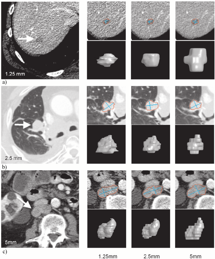
Figure 1: Examples of lesions in liver, lung and lymph nodes on 1.25, 2.5 and 5 mm slice interval images adopt from [31]. The left panel shows a close-up of (a) liver metastasis on a 1.25 mm slice interval image, (b) lung lesion on a 2.5 mm image, and (c) lymph node metastasis on a 5 mm image. The right panel shows the computer-aided contour, 2 maximal perpendicular diameters and three-dimensional views of each lesion on (from left to right, respectively) 1.25, 2.5 and 5 mm slice intervals.

I-B Super-Resolution

To get the best from both worlds, one potential strategy is the use of post-processing super-resolution (SR) algorithms. These algorithms are capable of generating high-resolution (HR) thin-slice CT images from low-resolution (LR) thick-slice CT images. Image SR is a sub-field of image processing that aims to generate a HR image from its corresponding LR counterpart. It is typically formulated as an inverse problem. The relationship between a LR image $Y$ and its corresponding HR image $X$ is often described using the following equation:

$${I_{LR}}=D\cdot S\cdot{I_{HR}}+N$$ (1)

Where $S$ is the downsampling operator, $D$ is the blurring operator (which represents the real-world degradation that often occurs when an image is captured), and $N$ is the noise. The aim of SR is to reverse this process, effectively trying to find the inverse of ${D}({S}(\cdot)+{N})$ to generate a super-resolved image ${I^{\prime}_{HR}}$ that is an approximation of the original ${I_{HR}}$. Ideally, we want ${I^{\prime}_{HR}}$ to minimize some loss function $L$ over inverse function parameters $\theta$ with respect to ${I_{HR}}$:

$${\hat{\theta}}=\arg\min_{{\theta}}L({I^{\prime}_{HR}},{I_{HR}})$$ (2)

In practice, ${I_{HR}}$ is unknown during the inference phase, and the model is trained on pairs of HR and LR images to learn the mapping from ${I_{LR}}$ to ${I_{HR}}$. A myriad of machine learning and deep learning models have been put forth to tackle the challenge of axial-plane SR. However, the lack of publicly available paired LR-HR training data forces researchers to create their own thick-slice CT images derived from thin-slice CT datasets. Regrettably, their simulation methods often overlook the crucial parameters of slice thickness and interval, leading to an inability to accurately capture the distribution of thick-slice images. This results in underperformance of the trained models when processing true thick-slice images.

I-C Aims and Objectives

The objective of this research is to present an innovative simulation algorithm that generates images closely resemble the actual thick-slice CT images found in the AAPM-Mayo’s 2016 Low Dose CT Grand Challenge (LDCT) dataset [34]. According to our current understanding, the AAPM-Mayo’s LDCT dataset stands as the sole public resource providing thin-thick slice pairs. We intend to utilise metrics such as the Peak Signal-to-Noise Ratio (PSNR) and the Root Mean Square Error (RMSE) to evaluate the quality of thick-slice images generated by different algorithms. The initial hypothesis posits that our proposed simulation method will yield thick-slice images more congruent with their real counterparts. Furthermore, a secondary hypothesis suggests that Super Resolution (SR) models trained on our dataset will demonstrate enhanced efficacy when applied to actual thick-slice images, in contrast to models trained on alternative simulated data. The evaluation of the SR model’s performance will also leverage PSNR and RMSE metrics.

II Related Works

Deep learning [35] has revolutionized the field of medical imaging super-resolution by enabling models to learn complex mappings from low to high-resolution images. Convolutional Neural Networks (CNNs) [36] and Generative Adversarial Networks (GANs) [37] are commonly used architectures in these tasks. These models are typically trained on pairs of low and high-resolution medical images, learning a function that can effectively upscale the low-resolution images. Their capacity to learn hierarchical features allows for the reconstruction of fine details in high-resolution images. Mansoor et al. [38] applied a 3D Gaussian smoothing filter on slices with 1mm thickness followed by downsampling to create slices with 4mm thickness on their in-house chest CT dataset. Subsequently, they utilized a VGG-like GAN model for the reconstruction of HR thin-slice images. Park et al. [39] employed a method for thick-slice image simulation that involved averaging five slices with a 3mm thickness to create a single slice with a 15mm slice thickness on their in-house Brain CT dataset. In this approach, the middle slice was selected as the ground truth high-resolution image. To reconstruct the HR thin-slice image from the LR thick-slice images, they employed a 2-D U-Net model. Wang et al. [40] generated thick slices by downsampling directly on the 1mm thin-slice images. They trained a CycleGAN in a self-supervised manner to recover the HR image. Xie et al. [41] employed a method for simulating thick-slice images by averaging three or seven slices with a 1mm thickness from their in-house brain CT dataset. This averaging process resulted in the creation of a single slice with a thickness of 3mm or 7mm, respectively. Additionally, they implemented a self-supervised CycleGAN model to synthesize HR thin-slice images. Park et al. [42] utilized a direct reconstruction approach from the sinogram in their in-house dataset to generate CT images with slice thicknesses of 1mm, 3mm, and 5mm. Their findings highlighted a significant variability in radiomic features across different CT slice thicknesses, particularly in the context of lung cancer. To address this variability, they proposed the use of a residual CNN-based SR algorithm. Wu et al. [43] simulated thick slices by downsampling directly on the 2.5mm thin-slice images. They proposed a parallel U-net architecture for CT slice reconstruction along the z-axis. Kudo et al. [44] simulated various combinations of slice thickness and slice interval by reducing the number of slices to either 1/4 or 1/8. They applied spline interpolation and random Gaussian noise to the reduced slices and utilized a 3D GAN model to convert the thick-slice images back to thin-slice images. In summary, prior simulation methodologies predominantly fall into three categories: Simple Averaging, Gaussian Averaging, and Direct Downsampling. Furthermore, the super-resolution models employed in these studies typically rely on CNN-based and GAN-based frameworks.

III Methods

III-A Dataset

This study principally utilized two data sets: the TCIA LDCT-and-Projection-data [45] and the 2016 Low Dose CT Grand Challenge [34]. We simulated thick-slice data based on the TCIA LDCT-and-Projection-data, employing it for the training phase. The 2016 Low Dose CT Grand Challenge was then deployed for testing purposes. Important features of these two datasets have been compiled and are presented in Table I and Table II for reference.

III-A1 TCIA LDCT-and-Projection-data

This compilation includes 99 neuro scans (denoted by N), 100 chest scans (denoted by C), and 100 liver scans (denoted by L). Half of each scan category comes from a SOMATOM Definition Flash CT scanner, a product of Siemens Healthcare from Forchheim, Germany. The remaining scans, consisting of 49 for the head, 50 for the chest, and 50 for the liver, were captured with a Lightspeed Volume Computed Tomography (VCT) CT scanner from GE Healthcare, based in Waukesha, WI. Some data in this collection might be utilized to reconstruct a human face. In order to protect the privacy of individuals involved, those accessing the data are required to sign and submit a TCIA Restricted License Agreement upon usage.

TABLE I: Key data acquisition parameters for each exam type in TCIA LDCT-and-Projection-data

Scanner	Parameters	Head CT (N)	Chest CT (C)	Abdomen CT (L)
GE Healthcare (Discovery CT750i)	Tube Potential (kV)	120	80-120	80-120
	Contrast Enhanced	No	No	Yes
	Field of View	200-260	282-423	315-500
	Reconstruction Algorithm	Standard	Standard	Standard
	Thickness/Increment (mm)	5/5	1.25/1	5/3
Siemens Healthineers (SOMATOM Definition AS+, SOMATOM Definition Flash)	Tube Potential (kV)	120	120	100-120
	Contrast Enhanced	No	No	Yes
	Field of View	250	300-350	300-350
	Reconstruction Kernel	H40	B50	B30
	Thickness/Increment (mm)	5/5	1.5/1	5/3

III-A2 2016 Low Dose CT Grand Challenge

The dataset consists of 30 deidentified contrast-enhanced abdominal CT patient scans, which were obtained using a Siemens SOMATOM Flash scanner in the portal venous phase. The data comprises two types: Full Dose (FD) data and Quarter Dose (QD) data. Full Dose data corresponds to scans acquired at 120 kV and 200 quality reference mAs (QRM), while Quarter Dose data refers to simulated scans acquired at 120 kV and 50 QRM. The provided dataset includes various components: 1) Projection data for all 30 patient scans, including 10 cases for training purposes (both FD and QD) and 20 cases for testing (QD only). 2) DICOM images for the 10 training cases, encompassing FD and QD data, with reconstructions using 1 mm thick B30 and D45 kernels, as well as 3 mm thick B30 and D45 kernels. 3) DICOM images for the 20 testing cases, consisting of QD data only, with the same reconstruction configurations as the training cases (1 mm thick B30 and D45 kernels, and 3 mm thick B30 and D45 kernels).

TABLE II: Key data acquisition parameters for each exam type in 2016 Low Dose CT Grand Challenge

Reconstruction Kernel	Parameters	Full Dosage (FD)	Quarter Dosage (QD)
D45	Tube Potential (kV)	100-120	100-120
	Tube Current (mAs)	200	50
	Contrast Enhanced	Yes	Yes
	Thickness/Increment (mm)	1/0.8 and 3/2	1/0.8 and 3/2
B30	Tube Potential (kV)	100-120	100-120
	Tube Current (mAs)	200	50
	Contrast Enhanced	Yes	Yes
	Thickness/Increment (mm)	1/0.8 and 3/2	1/0.8 and 3/2

III-B Evaluation Metrics

The Peak Signal-to-Noise Ratio (PSNR) and the Root Mean Square Error (RMSE) are two popular metrics used to measure the quality of image, particularly for comparing the differences between the original and reconstructed data. PSNR is defined as the ratio between the maximum possible power of a signal and the power of corrupting noise that affects the fidelity of its representation. Mathematically, PSNR is calculated using the following formula:

$$PSNR=20\cdot\log_{10}\left(\frac{MAX_{I}}{\sqrt{MSE}}\right)$$ (3)

Where $MAX_{I}$ is the maximum possible pixel value of the image. $MSE$ stands for Mean Squared Error, which is the mean of the squared differences between the original and the reconstructed image. The mathematical expression is as follows:

$$MSE=\frac{1}{mn}\sum_{i=0}^{m}\sum_{j=0}^{n}(I(i,j)-\hat{I}(i,j))^{2}$$ (4)

where, $I(i,j)$ is the original value, $\hat{I}(i,j)$ is the predicted value, and $m\times n$ is the image dimension (i.e. total number of pixels in an image). RMSE is a quadratic scoring rule that measures the average magnitude of the error, and it is defined as the square root of the average of squared differences between prediction and actual observation. The RMSE gives a relatively high weight to large errors, so it is especially useful when large errors are particularly undesirable. It can be calculated using equation 4:

$$RMSE=\sqrt{MSE}$$ (5)

Both PSNR and RMSE are higher-is-better metrics, with higher values indicating better match between the original and reconstructed data.

III-C Thick-slice Simulation

Drawing inspiration from the Weighted Filter Backprojection (wFBP) [46], we have crafted a weighted sum algorithm designed to simulate thick-slice images from thin-slice counterparts. Our initial step involves determining the new positions of the simulated-thick slices, which is based on the slice increment, $d$. This process is concisely delineated in Algorithm 1.

Algorithm 1 Slice location algorithm

1:start $s$, end $e$, slice increment $d$

2:slice locations $L_{\text{thick}}$

3:direction $D\leftarrow\frac{e-s}{|e-s|}$

4:Initialize $L_{\text{thick}}=[]$

5:$p\leftarrow s$

6:if $s=e$ then

7:     Append $s$ to $L_{\text{thick}}$

8:else

9:     while $(D=1\land s\leq p\leq e)\lor(D=-1\land e\leq p\leq s)$ do

10:         Append $p$ to $L_{\text{thick}}$

11:         $p\leftarrow p+D\cdot d$

12:     end while

13:end if

Subsequently, our focus shifts to estimating the extent to which contiguous thin-slice images at location $l\in L_{\text{thin}}$ contribute to the reconstruction of the thick-slice image at location $p\in L_{\text{thick}}$. To this end, we define a triangular weight function $g(s)$, where $s$ represents the slice thickness:

$$g(s)=\max\left(0,1-\frac{{\left|p-l\right|}}{s}\right)$$ (6)

The generated thick slices are weighted sums of the thin slices, normalized by the total weight of the slices used. The detailed steps for the generation of thick-slice images is illustrated in Algorithm 2. We applied our simulation algorithm to the 2016 Low Dose CT Grand Challenge dataset, thereby establishing the superior efficacy of our method compared to existing alternatives. Subsequently, we produced thick-slice data for the chest CT images from the TCIA LDCT-and-Projection-data dataset using Simple Averaging and our proposed method. These synthesized thick-thin image pairs served as the training set for the super-resolution models.

Algorithm 2 Weighted Sum of Images

1:$L_{\text{thick}}$ (thick-slice locations), $\bm{I}_{\text{thin}}\in\mathbb{R}^{512\times 512\times\text{depth}}$ (thin-slice images), $s$ (slice thickness)

2:$\bm{I}_{\text{thick}}\in\mathbb{R}^{512\times 512\times\text{depth}}\leftarrow$ Initialize With Zeros(depth of $L_{thick}$)

3:for each $l$ in $L_{\text{thick}}$ do

4:     $w_{\text{total}}\leftarrow$ 0

5:     for each $\bm{i}\in\mathbb{R}^{512\times 512}$ in $\bm{I}_{\text{thin}}$ do

6:         $w\leftarrow$ $g(s)$

7:         if $w=0$ then

8:              continue

9:         end if

10:         $\tilde{i}\leftarrow\tilde{i}+i\cdot w$

11:         $w_{\text{total}}\leftarrow$ $w_{\text{total}}+w$

12:     end for

13:     $\tilde{i}\leftarrow$ $\frac{1}{w_{\text{total}}}\cdot\tilde{i}$

14:     Append $\tilde{i}$ to $\bm{I}_{\text{thick}}$ along the depth dimension

15:end for

16:return $\bm{I}_{\text{thick}}$

III-D Super-Resolution Models

To fairly evaluate the quality of our simulated dataset in model training, We selected four SR models to benchmark our simulated thick-slice data.

III-D1 Convolutional Neural Network

Convolutional Neural Networks (CNNs), a class of artificial neural networks, have been instrumental in the evolution of deep learning, particularly in image analysis tasks. The basic underlying principle of CNNs is the application of a convolution operation, which uses a kernel or filter that passes over the input data. This kernel convolves with the input layer to compute the dot product of their entries, thereby preserving the spatial relationships in the image. Layers of these convolutional operations are often interspersed with other layers such as pooling (downsampling) and normalization layers. Over time, the CNN learns the optimal values for this kernel, allowing it to detect complex patterns in the input data. CNN-based Super-Resolution models revolutionized this field, with the most famous being the Super-Resolution Convolutional Neural Network (SRCNN) introduced by Dong et al. in 2014 [47]. This model uses a three-layer CNN to learn an end-to-end mapping of low-resolution images to their high-resolution counterparts. It applies a patch extraction and representation layer, a non-linear mapping layer, and a reconstruction layer. The learning objective of SRCNN is to minimize the Mean Squared Error (MSE) between the original high-resolution image and the super-resolved output. Since then, newer models like the very Deep Super-Resolution (VDSR) [48] have further improved super-resolution performance. We have re-engineered the VDSR architecture to better suit our needs, transforming all 2-D operations into 3-D. Further, we streamlined the structure by reducing the convolutional layer count to twelve and integrated a global residual connection. This refined model will serve as our first SR model for benchmarking our simulated dataset.

III-D2 U-Net

U-Net [49], a type of CNN that was first developed for biomedical image segmentation, has also been utilized in super-resolution tasks due to its unique architecture that excels in capturing both local features and global context. The U-Net architecture consists of a contracting (downsampling) path and an expansive (upsampling) path with skip connections between layers of the same level, which help in localizing the high resolution features. One example of a U-Net-based super-resolution model is the Enhanced Deep Residual Networks for Single Image Super-Resolution (EDSR) model [50] that’s been adapted into a U-Net-like structure. In this model, the downsampling path captures context information, while the upsampling path allows the model to make precise localization decisions to super-resolve the image. We have adapted the original U-Net architecture to better suit the 3-D medical image super-resolution task. Our modifications include transforming all 2-D operations into 3-D and introducing two additional residual blocks. This revised model now serves as our second benchmark SR model.

III-D3 Residual Neural Nerwork

ResNet, short for Residual Network, was introduced by He et al. in their 2015 paper [51]. This deep learning model, distinguished by its ”skip” or ”shortcut” connections, was developed to address the problem of vanishing gradients that plagued training of very deep neural networks. These shortcut connections allow the model to learn identity functions that effectively prevent the higher layers from destroying the learned information of lower layers, thereby enabling the successful training of networks that are significantly deeper than those previously possible. ResNet has had a significant impact on the field of computer vision, including the domain of super-resolution. SRResNet, or Super-Resolution Residual Network, is a direct adaptation of the principles of ResNet to super-resolution tasks. SRResNet was proposed by Ledig et al. in the SRGAN (Super-Resolution Generative Adversarial Networks) paper and serves as the backbone for the generator network in SRGAN [52]. SRResNet incorporates residual blocks to learn the residual mapping between the low-resolution and high-resolution images. It is designed with a shallow network at the beginning and end (for feature extraction and reconstruction) while having a deeper body composed of residual blocks. Building upon the success of SRResNet, researchers proposed an enhanced version known as Enhanced SRResNet (ESRResNet) [53]. The enhanced version incorporates several advancements in deep learning, like the use of dense connections (as seen in DenseNet [54]) and parameter-efficient convolutions to improve the network’s learning capacity while keeping the computational load manageable. In addition, one key feature of the ESRResNet is the use of Residual-in-Residual Dense Blocks (RRDBs) instead of the simple residual blocks in the original SRResNet. The RRDB is essentially a stack of residual blocks where the output of each residual block is added to its input (forming a local skip connection), and the output of the last residual block in the stack is also added to the input of the stack (forming a long skip connection). This architecture allows for better propagation of features and gradients through the network, making it easier for the network to learn the mapping from low-resolution to high-resolution images. The ESRResNet has proven to be highly effective in super-resolution tasks, leading to significant improvements over the original SRResNet in terms of both quantitative metrics and perceptual quality of the super-resolved images. Consequently, we selected the ESRResNet architecture, modifying all its 2-D operations to 3-D. This adaptation makes it more suitable for the specific demands of the medical imaging super-resolution task. This adaptation now constitutes our third super-resolution model for benchmarking purposes.

III-D4 Generative Adversarial Network

Generative Adversarial Networks (GANs) are a type of neural network architecture introduced by Ian Goodfellow et al. in 2014 [37]. GANs consist of two parts: a generator network, which produces synthetic data, and a discriminator network, which tries to distinguish between real and synthetic data. The two networks are trained together, with the generator network attempting to produce data that the discriminator network cannot distinguish from real data, and the discriminator network attempting to get better at distinguishing real data from the data generated by the generator. This adversarial process leads to the generator network producing high-quality synthetic data. In the context of image super-resolution, GANs have shown great potential. Ledig et al. introduced the Super-Resolution Generative Adversarial Network (SRGAN) in 2016 [52], which uses a GAN in combination with a super-resolution network (SRResNet, described in section III-D3). In this architecture, the generator is a super-resolution model that transforms a low-resolution input into a high-resolution output, and the discriminator is trained to distinguish the super-resolved images from real high-resolution images. The result is super-resolved images that are perceptually more similar to real high-resolution images compared to those produced by traditional super-resolution methods. ESRGAN [53], or Enhanced Super-Resolution Generative Adversarial Networks, is a direct and substantial improvement of SRGAN. It keeps the GAN structure of the original SRGAN model, with a generator and discriminator, but upgrades the generator with RRDB (desribed in section III-D3). RRDB allows the model to effectively capture more complex texture and detail information by encouraging both short and long skip connections. The discriminator in these networks is typically constructed as a deep CNN, with several layers of convolution, batch normalization, and activation function such as LeakyReLU, culminating in a final decision layer that outputs a probability indicating how likely it is that the input image is real. There are more advanced architectures such as PatchGAN [55]. Unlike traditional discriminators that try to classify the entire image as real or fake, a PatchGAN discriminator employs the concept of Markov Random Field and classifies individual patches of an image. The underlying assumption is that natural images are locally coherent, meaning that the authenticity of an image can be determined by examining its subregions or patches. In this study, we included the PatchGAN discriminator during the training of ESRResNet, adding it as our fourth SR model for benchmarking.

III-E Implementation Details

The scripts used in this study were developed in Python3 and the PyTorch framework, executed on Imperial College’s HPC Clusters. Computations were run on an NVIDIA RTX 6000 GPU with 24 GB of memory. Four distinct Super Resolution (SR) models: VDSR, U-Net, ESRResNet and ESRGAN (ESRResNet+PatchGAN Discriminator), were trained over 1000 epochs using the Adam solver (learning rate = 1e-4) and augmented with random horizontal flips during training. The source code can be accessed at: https://github.com/Feanor007/Thick2Thin.

IV Results

The results from all conducted experiments, represented as mean $\pm$ standard deviation, are tabulated in this section. We assessed the performance of our proposed simulation method against Simple Averaging, Gaussian Averaging, and Direct Downsampling. This was accomplished by simulating images with a thickness of 3mm from those with a thickness of 1mm, utilizing the 2016 Low Dose CT Grand Challenge dataset. The results outlined in Table III provide a comparative analysis of different thick-slice simulation methods used in two datasets from the 2016 Low Dose CT Grand Challenge. Both the PSNR and the RMSE were used as key performance indicators for these methods. The data clearly demonstrate that the proposed method significantly outperformed Simple Averaging, Gaussian Averaging, and Direct Downsampling in both datasets (D45 and B30). The highest PSNR values were obtained with the proposed method, yielding 49.7369 $\pm$ 2.5223 and 48.5801 $\pm$ 7.3271 for D45 and B30 datasets, respectively. The proposed method also registered the lowest RMSE with values of 0.0068 $\pm$ 0.0020 and 0.0108 $\pm$ 0.0099 for D45 and B30, respectively. These results indicate a superior level of accuracy and reliability in the proposed method. The statistically significant differences were confirmed by a Wilcoxon signed-rank test with p-value ¡ 0.05, implying that the improvements from the proposed method were not due to random chance. These findings support our first hypothesis that the proposed simulation method provides a more efficient and precise approach to thick-slice simulations compared to traditional methods. To provide a more comprehensive evaluation, visual comparisons from axial, coronal and sagittal plane were also undertaken, as depicted in Figures 2 to 4. In summary, Our proposed method demonstrated substantial enhancements in terms of both PSNR and RMSE, indicating a distribution more closely aligned with the authentic thick-slice image.

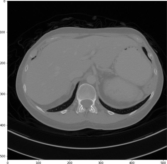
(a) True Thick-slice image

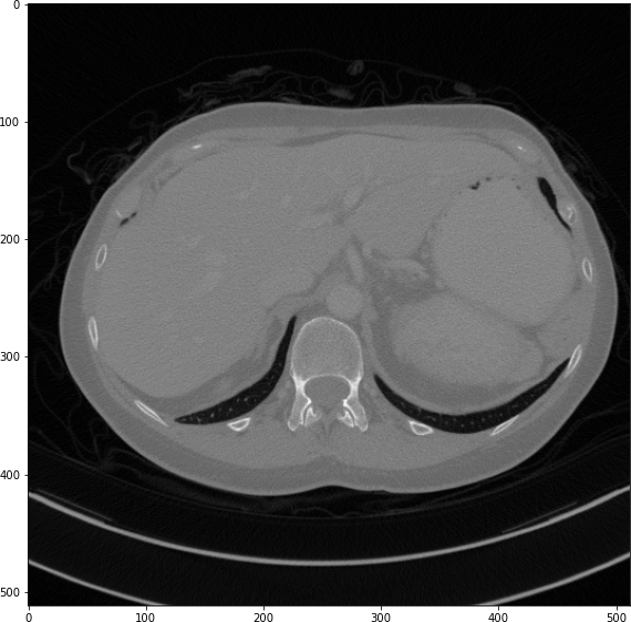
(b) Simple Averaging
RMSE: 0.0329, PSNR: 35.6776

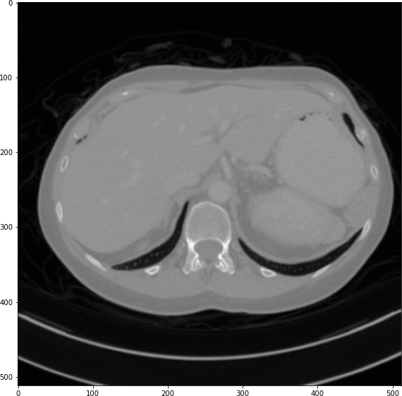
(c) Gaussian Averaging
RMSE: 0.0955, PSNR: 26.4221

(d) Direct Downsampling
RMSE: 0.0454, PSNR: 32.8776

(e) Proposed Simulation
RMSE: 0.0010, PSNR: 46.4076

Figure 2: Axial-plane thick-slice image quality comparison across four simulation methods.

(a) True Thick-slice image

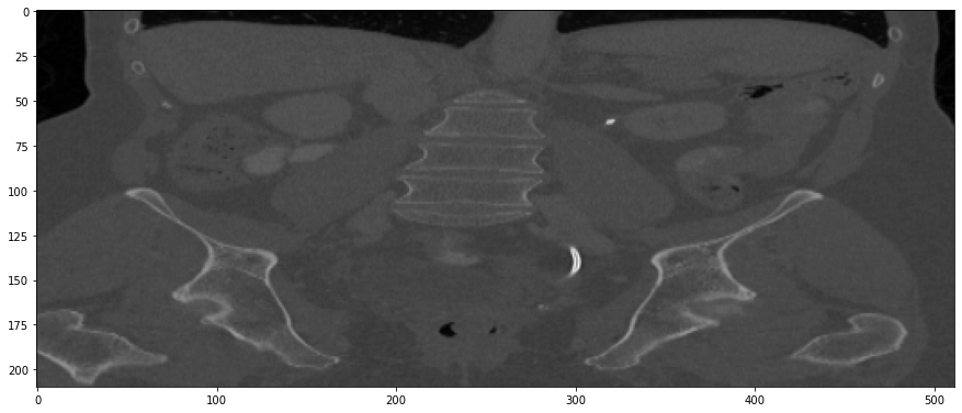
(b) Simple Averaging
RMSE: 0.0250, PSNR: 38.0530

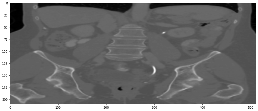
(c) Gaussian Averaging
RMSE: 0.1758, PSNR: 21.1182

(d) Direct Downsampling
RMSE: 0.0348, PSNR: 35.1697

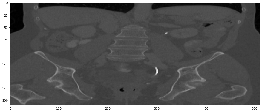
(e) Proposed Simulation
RMSE: 0.0051, PSNR: 51.8504

Figure 3: Coronal-plane thick-slice image quality comparison across four simulation methods.

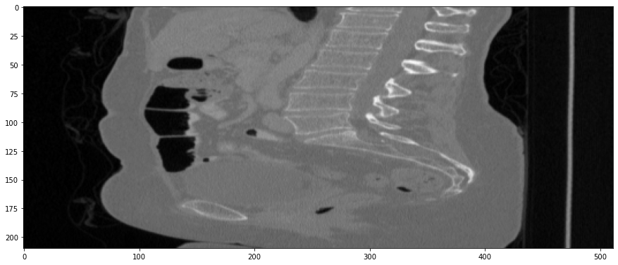
(a) True Thick-slice image

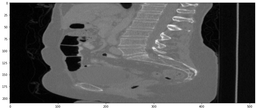
(b) Simple Averaging
RMSE: 0.0357, PSNR: 34.9781

(c) Gaussian Averaging
RMSE: 0.0454, PSNR: 32.8866

(d) Direct Downsampling
RMSE: 0.0486, PSNR: 32.2861

(e) Proposed Simulation
RMSE: 0.0070, PSNR: 49.1774

Figure 4: Sagittal-plane thick-slice image quality comparison across four simulation methods.

TABLE III: Comparison experiments on different thick-slice simulation methods

Dataset	Simulation Methods	PSNR	RMSE
2016 Low Dose CT Grand Challenge (D45)	Simple Averaging	38.5023 $\pm$ 2.5851$\dagger$	0.0249 $\pm$ 0.0081$\dagger$
	Gaussian Averaging	30.0969 $\pm$ 5.0047$\dagger$	0.0746 $\pm$ 0.0484$\dagger$
	Direct Downsampling	36.0757 $\pm$ 2.9024$\dagger$	0.0334 $\pm$ 0.0131$\dagger$
	Proposed	49.7369 $\pm$ 2.5223	0.0068 $\pm$ 0.0020
2016 Low Dose CT Grand Challenge (B30)	Simple Averaging	39.6945 $\pm$ 2.8208$\dagger$	0.0219 $\pm$ 0.0072$\dagger$
	Gaussian Averaging	33.4242 $\pm$ 4.9641$\dagger$	0.0521 $\pm$ 0.0412$\dagger$
	Direct Downsampling	36.2342 $\pm$ 3.3025$\dagger$	0.0334 $\pm$ 0.0150$\dagger$
	Proposed	48.5801 $\pm$ 7.3271	0.0108 $\pm$ 0.0099

• represents statistical significance (with Wilcoxon signed-rank test p-value ¡ 0.05) compared with the proposed method.

We investigated our second hypothesis by training four different SR models using the data generated by top two simulation methods, as referenced in III, which are our proposed method and Simple Averaging. The results in Table IV highlight the comparison of various super-resolution (SR) models trained by different simulation methods on two distinct datasets: 2016 Low Dose CT Grand Challenge (D45 and B30). In each case, the performance of the SR model trained by proposed simulation method outperforms itself trained by the Simple Averaging simulation method in terms of both PSNR and RMSE, indicating improved image quality and lower error rates, respectively. The differences observed were statistically significant as determined by the Wilcoxon signed-rank test (p-value ¡ 0.05). For the D45 dataset, the PSNR and RMSE of the proposed method ranged from 37.2176 $\pm$ 3.0876 and 0.0296 $\pm$ 0.0128 (for VDSR) to 37.9786 $\pm$ 2.4597 and 0.0264 $\pm$ 0.0089 (for ESRGAN). Similarly, for the B30 dataset, the proposed method’s PSNR and RMSE varied between 38.5657 $\pm$ 4.6613 and 0.0280 $\pm$ 0.0196 (for VDSR) and 40.5083 $\pm$ 3.8736 and 0.0215 $\pm$ 0.0144 (for ESRGAN). The SR model that demonstrated the best performance using the proposed method on the B30 dataset was the ESRGAN model, yielding the highest PSNR (40.5083 $\pm$ 3.8736) and the lowest RMSE (0.0215 $\pm$ 0.0144). In contrast, the lowest performance in the proposed method was observed in the VDSR model for the D45 dataset, exhibiting the lowest PSNR (37.2176 $\pm$ 3.0876) and the highest RMSE (0.0296 $\pm$ 0.0128). Regardless of the dataset and the SR model, the proposed simulation method consistently outperformed the simple averaging method, signifying its effectiveness in training super-resolution models in the task of thick-to-thin CT image transformation.

TABLE IV: Comparison experiments on models trained by different simulated thick-slice images

Dataset	Super-Resolution Model	Simulation Methods	PSNR	RMSE
2016 Low Dose CT	VDSR	Simple Averaging	36.4722 $\pm$ 2.9112$\dagger$	0.0320 $\pm$ 0.0131$\dagger$
Grand Challenge (D45)		Proposed	37.2176 $\pm$ 3.0876	0.0296 $\pm$ 0.0128
	U-Net	Simple Averaging	36.5079 $\pm$ 2.9129$\dagger$	0.0319 $\pm$ 0.0133$\dagger$
		Proposed	37.9405 $\pm$ 2.1842	0.0262 $\pm$ 0.0071
	ESRResNet	Simple Averaging	36.6322 $\pm$ 2.7383$\dagger$	0.0312 $\pm$ 0.0120$\dagger$
		Proposed	37.8946 $\pm$ 2.5350	0.0267 $\pm$ 0.0094
	ESRGAN	Simple Averaging	36.8371 $\pm$ 2.4522$\dagger$	0.0301 $\pm$ 0.0098$\dagger$
		Proposed	37.9786 $\pm$ 2.4597	0.0264 $\pm$ 0.0089
2016 Low Dose CT	VDSR	Simple Averaging	37.2458 $\pm$ 4.6983$\dagger$	0.0323 $\pm$ 0.0209$\dagger$
Grand Challenge (B30)		Proposed	38.5657 $\pm$ 4.6613	0.0280 $\pm$ 0.0196
	U-Net	Simple Averaging	37.4172 $\pm$ 4.4380$\dagger$	0.0311 $\pm$ 0.0185$\dagger$
		Proposed	39.7475 $\pm$ 3.5318	0.0226 $\pm$ 0.0112
	ESRResNet	Simple Averaging	37.9217 $\pm$ 4.1180$\dagger$	0.0289 $\pm$ 0.0171$\dagger$
		Proposed	40.2103 $\pm$ 3.9283	0.0223 $\pm$ 0.0150
	ESRGAN	Simple Averaging	38.2401 $\pm$ 3.6225$\dagger$	0.0270 $\pm$ 0.0136$\dagger$
		Proposed	40.5083 $\pm$ 3.8736	0.0215 $\pm$ 0.0144

• represents statistical significance (with Wilcoxon signed-rank test p-value ¡ 0.05) compared with the proposed method.

V Discussion and Conclusion

The findings from our study underscore the potential effectiveness of our proposed simulation algorithm in generating images that closely resemble authentic thick-slice CT images from the AAPM-Mayo’s 2016 Low Dose CT Grand Challenge dataset. According to the comparison metrics used, specifically PSNR and RMSE, our proposed method presented a significant improvement over previous simulation methods, implying an image distribution more closely aligned with the actual thick-slice images. This superior performance over the other methods (Simple Averaging, Gaussian Averaging and Direct Downsampling) demonstrates its potential as a reliable tool for training super-resolution (SR) models for the task of thick-to-thin CT image transformation. The positive results reaffirm our initial hypothesis and add to the growing body of evidence that highlights the importance of using high-fidelity simulated data in training deep learning models, especially in the realm of medical imaging. However, it is essential to acknowledge the limitations of our study. One of the significant limitations stems from the reliance on the AAPM-Mayo’s LDCT dataset, which, to the best of our knowledge, is the only public resource providing thin-thick slice pairs. The performance of our proposed method has been evaluated primarily with respect to recreating the specific image characteristics of the AAPM-Mayo’s LDCT dataset. It remains unclear how well our algorithm would perform with images obtained from patients with different health conditions. Furthermore, its exclusive provision of 3mm-1mm thick-thin slice pairs, presents an inherent constraint in our study. In clinical settings, various slice thicknesses, including 5mm, 10mm, or even 15mm, are commonly used depending on the particularities of the clinical question and the body region being scanned. The unique features and details that are present in thicker slices may be vital for diagnosing certain conditions or predicting disease progression. If our algorithm has only been validated for a 3mm-1mm pairing, it remains uncertain how well it can generate and maintain these crucial features in thicker slices. In addition, the evaluation metrics used (PSNR and RMSE) may not fully capture perceptual image quality and radiomics features as perceived by human experts, thereby potentially limiting the perceived accuracy of the simulation. Looking forward, further research could explore more advanced SR models, such as diffusion-based generative models [56]. Additionally, researchers could validate the utility of super-resolved CT images by applying segmentation models that delineate anatomical structures such as airway tree [57] and lung nodules [58]. Finally, these results should prompt a reconsideration of the role of simulated data in training SR models, urging further exploration and innovation in this area. By providing a robust simulation method, we can help ensure the best possible data for training these models, which in turn has the potential to improve the overall quality and accuracy of medical imaging, particularly in the realm of CT scanning.

In conclusion, this study successfully presented an innovative simulation algorithm capable of generating thick-slice CT images closely resembling the actual images in the AAPM-Mayo’s 2016 Low Dose CT Grand Challenge dataset. Furthermore, Our method demonstrated its potential utility for training super-resolution models aimed at the task of thick-to-thin CT image transformation.

References

- [1] I. Mori, “Computerized tomographic apparatus utilizing a radiation source,” US Patent 4 630 202, 1986.
- [2] H. Nishimura and O. Miyazaki, “Ct system for spirally scanning subject on a movable bed synchronized to x-ray tube revolution,” US Patent 4 789 929, 1988.
- [3] C. R. Crawford and K. F. King, “Computed tomography scanning with simultaneous patient translation,” Medical Physics, vol. 17, no. 6, pp. 967–982, Nov. 1990. [Online]. Available: https://doi.org/10.1118/1.596464
- [4] W. A. Kalender, W. Seissler, E. Klotz, and P. Vock, “Spiral volumetric CT with single-breath-hold technique, continuous transport, and continuous scanner rotation.” Radiology, vol. 176, no. 1, pp. 181–183, Jul. 1990. [Online]. Available: https://doi.org/10.1148/radiology.176.1.2353088
- [5] J. Rydberg, K. A. Buckwalter, K. S. Caldemeyer, M. D. Phillips, D. J. Conces, A. M. Aisen, S. A. Persohn, and K. K. Kopecky, “Multisection CT: Scanning techniques and clinical applications,” RadioGraphics, vol. 20, no. 6, pp. 1787–1806, Nov. 2000. [Online]. Available: https://doi.org/10.1148/radiographics.20.6.g00nv071787
- [6] L. W. Goldman, “Principles of CT: Multislice CT,” Journal of Nuclear Medicine Technology, vol. 36, no. 2, pp. 57–68, May 2008. [Online]. Available: https://doi.org/10.2967/jnmt.107.044826
- [7] H. Hu, “Multi-slice helical CT: Scan and reconstruction,” Medical Physics, vol. 26, no. 1, pp. 5–18, Jan. 1999. [Online]. Available: https://doi.org/10.1118/1.598470
- [8] C. V. Zwirewich, S. Vedal, R. R. Miller, and N. L. Müller, “Solitary pulmonary nodule: high-resolution CT and radiologic-pathologic correlation.” Radiology, vol. 179, no. 2, pp. 469–476, May 1991. [Online]. Available: https://doi.org/10.1148/radiology.179.2.2014294
- [9] C. I. Henschke, D. I. McCauley, D. F. Yankelevitz, D. P. Naidich, G. McGuinness, O. S. Miettinen, D. M. Libby, M. W. Pasmantier, J. Koizumi, N. K. Altorki, and J. P. Smith, “Early lung cancer action project: overall design and findings from baseline screening,” The Lancet, vol. 354, no. 9173, pp. 99–105, Jul. 1999. [Online]. Available: https://doi.org/10.1016/s0140-6736(99)06093-6
- [10] S. G. Armato, G. McLennan, L. Bidaut, M. F. McNitt-Gray, C. R. Meyer, A. P. Reeves, B. Zhao, D. R. Aberle, C. I. Henschke, E. A. Hoffman, E. A. Kazerooni, H. MacMahon, E. J. R. van Beek, D. Yankelevitz, A. M. Biancardi, P. H. Bland, M. S. Brown, R. M. Engelmann, G. E. Laderach, D. Max, R. C. Pais, D. P.-Y. Qing, R. Y. Roberts, A. R. Smith, A. Starkey, P. Batra, P. Caligiuri, A. Farooqi, G. W. Gladish, C. M. Jude, R. F. Munden, I. Petkovska, L. E. Quint, L. H. Schwartz, B. Sundaram, L. E. Dodd, C. Fenimore, D. Gur, N. Petrick, J. Freymann, J. Kirby, B. Hughes, A. V. Casteele, S. Gupte, M. Sallam, M. D. Heath, M. H. Kuhn, E. Dharaiya, R. Burns, D. S. Fryd, M. Salganicoff, V. Anand, U. Shreter, S. Vastagh, B. Y. Croft, and L. P. Clarke, “The lung image database consortium (LIDC) and image database resource initiative (IDRI): A completed reference database of lung nodules on CT scans,” Medical Physics, vol. 38, no. 2, pp. 915–931, Jan. 2011. [Online]. Available: https://doi.org/10.1118/1.3528204
- [11] E. A. Regan, J. E. Hokanson, J. R. Murphy, B. Make, D. A. Lynch, T. H. Beaty, D. Curran-Everett, E. K. Silverman, and J. D. Crapo, “Genetic epidemiology of COPD (COPDGene) study design,” COPD: Journal of Chronic Obstructive Pulmonary Disease, vol. 7, no. 1, pp. 32–43, Mar. 2010. [Online]. Available: https://doi.org/10.3109/15412550903499522
- [12] C. J. Galbán, M. K. Han, J. L. Boes, K. A. Chughtai, C. R. Meyer, T. D. Johnson, S. Galbán, A. Rehemtulla, E. A. Kazerooni, F. J. Martinez, and B. D. Ross, “Computed tomography-based biomarker provides unique signature for diagnosis of COPD phenotypes and disease progression,” Nature Medicine, vol. 18, no. 11, pp. 1711–1715, Oct. 2012. [Online]. Available: https://doi.org/10.1038/nm.2971
- [13] O. M. Mets, P. A. de Jong, B. van Ginneken, H. A. Gietema, and J. W. J. Lammers, “Quantitative computed tomography in COPD: Possibilities and limitations,” Lung, vol. 190, no. 2, pp. 133–145, Dec. 2011. [Online]. Available: https://doi.org/10.1007/s00408-011-9353-9
- [14] K. B. Baumgartner, J. M. Samet, C. A. Stidley, T. V. Colby, and J. A. Waldron, “Cigarette smoking: a risk factor for idiopathic pulmonary fibrosis.” American Journal of Respiratory and Critical Care Medicine, vol. 155, no. 1, pp. 242–248, Jan. 1997. [Online]. Available: https://doi.org/10.1164/ajrccm.155.1.9001319
- [15] A. U. Wells, S. R. Desai, M. B. Rubens, N. S. L. Goh, D. Cramer, A. G. Nicholson, T. V. Colby, R. M. du Bois, and D. M. Hansell, “Idiopathic pulmonary fibrosis,” American Journal of Respiratory and Critical Care Medicine, vol. 167, no. 7, pp. 962–969, Apr. 2003. [Online]. Available: https://doi.org/10.1164/rccm.2111053
- [16] D. A. Lynch, N. Sverzellati, W. D. Travis, K. K. Brown, T. V. Colby, J. R. Galvin, J. G. Goldin, D. M. Hansell, Y. Inoue, T. Johkoh, A. G. Nicholson, S. L. Knight, S. Raoof, L. Richeldi, C. J. Ryerson, J. H. Ryu, and A. U. Wells, “Diagnostic criteria for idiopathic pulmonary fibrosis: a fleischner society white paper,” The Lancet Respiratory Medicine, vol. 6, no. 2, pp. 138–153, Feb. 2018. [Online]. Available: https://doi.org/10.1016/s2213-2600(17)30433-2
- [17] P. Pape, A. H. Jensen, O. Bergdal, T. N. Munch, S. S. Rudolph, and L. S. Rasmussen, “Time to CT scan for patients with acute severe neurological symptoms: a quality assurance study,” Scientific Reports, vol. 12, no. 1, Sep. 2022. [Online]. Available: https://doi.org/10.1038/s41598-022-19512-x
- [18] V. Vishwanath, S. Jafarieh, and A. Rembielak, “The role of imaging in head and neck cancer: An overview of different imaging modalities in primary diagnosis and staging of the disease,” Journal of Contemporary Brachytherapy, vol. 12, no. 5, pp. 512–518, 2020. [Online]. Available: https://doi.org/10.5114/jcb.2020.100386
- [19] R. Grant, “Overview: brain tumour diagnosis and management/royal college of physicians guidelines,” Journal of Neurology, Neurosurgery & Psychiatry, vol. 75, no. suppl_2, pp. ii18–ii23, Jun. 2004. [Online]. Available: https://doi.org/10.1136/jnnp.2004.040360
- [20] H. W. Goo, “State-of-the-art CT imaging techniques for congenital heart disease,” Korean Journal of Radiology, vol. 11, no. 1, p. 4, 2010. [Online]. Available: https://doi.org/10.3348/kjr.2010.11.1.4
- [21] H. W. Goo, I.-S. Park, J. K. Ko, Y. H. Kim, D.-M. Seo, and J.-J. Park, “Computed tomography for the diagnosis of congenital heart disease in pediatric and adult patients,” The International Journal of Cardiovascular Imaging, vol. 21, no. 2-3, pp. 347–365, Apr. 2005. [Online]. Available: https://doi.org/10.1007/s10554-004-4015-0
- [22] E. R. V. Buechel and L. L. Mertens, “Imaging the right heart: the use of integrated multimodality imaging,” European Heart Journal, vol. 33, no. 8, pp. 949–960, Mar. 2012. [Online]. Available: https://doi.org/10.1093/eurheartj/ehr490
- [23] W. Brisbane, M. R. Bailey, and M. D. Sorensen, “An overview of kidney stone imaging techniques,” Nature Reviews Urology, vol. 13, no. 11, pp. 654–662, Aug. 2016. [Online]. Available: https://doi.org/10.1038/nrurol.2016.154
- [24] C. Karohl, L. D. Gascón, and P. Raggi, “Noninvasive imaging for assessment of calcification in chronic kidney disease,” Nature Reviews Nephrology, vol. 7, no. 10, pp. 567–577, Aug. 2011. [Online]. Available: https://doi.org/10.1038/nrneph.2011.110
- [25] A. Tunaci and E. Yekeler, “Multidetector row CT of the kidneys,” European Journal of Radiology, vol. 52, no. 1, pp. 56–66, Oct. 2004. [Online]. Available: https://doi.org/10.1016/j.ejrad.2004.03.033
- [26] H. K. Kang, Y. Y. Jeong, J. H. Choi, S. Choi, T. W. Chung, J. J. Seo, J. K. Kim, W. Yoon, and J. G. Park, “Three-dimensional multi–detector row CT portal venography in the evaluation of portosystemic collateral vessels in liver cirrhosis,” RadioGraphics, vol. 22, no. 5, pp. 1053–1061, Sep. 2002. [Online]. Available: https://doi.org/10.1148/radiographics.22.5.g02se011053
- [27] B. Ariff, C. R. Lloyd, S. Khan, M. Shariff, A. V. Thillainayagam, D. S. Bansi, S. A. Khan, S. D. Taylor-Robinson, and A. K. Lim, “Imaging of liver cancer,” World Journal of Gastroenterology, vol. 15, no. 11, p. 1289, 2009. [Online]. Available: https://doi.org/10.3748/wjg.15.1289
- [28] M. Kudo, “Imaging diagnosis of hepatocellular carcinoma and premalignant/borderline lesions,” Seminars in Liver Disease, vol. 19, no. 03, pp. 297–309, 1999. [Online]. Available: https://doi.org/10.1055/s-2007-1007119
- [29] L. He, Y. Huang, Z. Ma, C. Liang, C. Liang, and Z. Liu, “Effects of contrast-enhancement, reconstruction slice thickness and convolution kernel on the diagnostic performance of radiomics signature in solitary pulmonary nodule,” Scientific Reports, vol. 6, no. 1, Oct. 2016. [Online]. Available: https://doi.org/10.1038/srep34921
- [30] B. Zhao, Y. Tan, W. Y. Tsai, L. H. Schwartz, and L. Lu, “Exploring variability in CT characterization of tumors: A preliminary phantom study,” Translational Oncology, vol. 7, no. 1, pp. 88–93, Feb. 2014. [Online]. Available: https://doi.org/10.1593/tlo.13865
- [31] Y. Tan, P. Guo, H. Mann, S. E. Marley, M. L. J. Scott, L. H. Schwartz, D. C. Ghiorghiu, and B. Zhao, “Assessing the effect of CT slice interval on unidimensional, bidimensional and volumetric measurements of solid tumours,” Cancer Imaging, vol. 12, no. 3, pp. 497–505, 2012. [Online]. Available: https://doi.org/10.1102/1470-7330.2012.0046
- [32] M. J. Murphy, J. Balter, S. Balter, J. A. BenComo, I. J. Das, S. B. Jiang, C.-M. Ma, G. H. Olivera, R. F. Rodebaugh, K. J. Ruchala, H. Shirato, and F.-F. Yin, “The management of imaging dose during image-guided radiotherapy: Report of the AAPM task group 75,” Medical Physics, vol. 34, no. 10, pp. 4041–4063, Sep. 2007. [Online]. Available: https://doi.org/10.1118/1.2775667
- [33] M. S. C. .-. on ALARA for Occupationally-Exposed Individuals in Clinical Radiology and M. S. C. . on Operational Radiation Safety, Implementation of the Principle of as Low as Reasonably Achievable (ALARA) for Medical and Dental Personnel: Recommendations of the National Council on Radiation Protection and Measurements. National Council on Radiation, 1990, no. 107.
- [34] C. H. McCollough, A. C. Bartley, R. E. Carter, B. Chen, T. A. Drees, P. Edwards, D. R. Holmes, A. E. Huang, F. Khan, S. Leng, K. L. McMillan, G. J. Michalak, K. M. Nunez, L. Yu, and J. G. Fletcher, “Low-dose CT for the detection and classification of metastatic liver lesions: Results of the 2016 low dose CT grand challenge,” Medical Physics, vol. 44, no. 10, pp. e339–e352, Oct. 2017. [Online]. Available: https://doi.org/10.1002/mp.12345
- [35] I. J. Goodfellow, Y. Bengio, and A. Courville, Deep Learning. Cambridge, MA, USA: MIT Press, 2016, http://www.deeplearningbook.org.
- [36] Y. Lecun, L. Bottou, Y. Bengio, and P. Haffner, “Gradient-based learning applied to document recognition,” Proceedings of the IEEE, vol. 86, no. 11, pp. 2278–2324, 1998.
- [37] I. Goodfellow, J. Pouget-Abadie, M. Mirza, B. Xu, D. Warde-Farley, S. Ozair, A. Courville, and Y. Bengio, “Generative adversarial networks,” Communications of the ACM, vol. 63, no. 11, pp. 139–144, Oct. 2020. [Online]. Available: https://doi.org/10.1145/3422622
- [38] A. Mansoor, T. Vongkovit, and M. G. Linguraru, “Adversarial approach to diagnostic quality volumetric image enhancement,” in 2018 IEEE 15th International Symposium on Biomedical Imaging (ISBI 2018). IEEE, Apr. 2018. [Online]. Available: https://doi.org/10.1109/isbi.2018.8363591
- [39] J. Park, D. Hwang, K. Y. Kim, S. K. Kang, Y. K. Kim, and J. S. Lee, “Computed tomography super-resolution using deep convolutional neural network,” Physics in Medicine & Biology, vol. 63, no. 14, p. 145011, Jul. 2018. [Online]. Available: https://doi.org/10.1088/1361-6560/aacdd4
- [40] T. Wang, Y. Lei, Z. Tian, X. Tang, W. J. Curran, T. Liu, and X. Yang, “Synthesizing high-resolution CT from low-resolution CT using self-learning,” in Medical Imaging 2021: Physics of Medical Imaging, H. Bosmans, W. Zhao, and L. Yu, Eds. SPIE, Feb. 2021. [Online]. Available: https://doi.org/10.1117/12.2581080
- [41] H. Xie, Y. Lei, T. Wang, Z. Tian, J. Roper, J. D. Bradley, W. J. Curran, X. Tang, T. Liu, and X. Yang, “High through-plane resolution CT imaging with self-supervised deep learning,” Physics in Medicine & Biology, vol. 66, no. 14, p. 145013, Jul. 2021. [Online]. Available: https://doi.org/10.1088/1361-6560/ac0684
- [42] S. Park, S. M. Lee, K.-H. Do, J.-G. Lee, W. Bae, H. Park, K.-H. Jung, and J. B. Seo, “Deep learning algorithm for reducing CT slice thickness: Effect on reproducibility of radiomic features in lung cancer,” Korean Journal of Radiology, vol. 20, no. 10, p. 1431, 2019. [Online]. Available: https://doi.org/10.3348/kjr.2019.0212
- [43] S. Wu, M. Nakao, K. Imanishi, M. Nakamura, T. Mizowaki, and T. Matsuda, “Computed tomography slice interpolation in the longitudinal direction based on deep learning techniques: To reduce slice thickness or slice increment without dose increase,” PLOS ONE, vol. 17, no. 12, p. e0279005, Dec. 2022. [Online]. Available: https://doi.org/10.1371/journal.pone.0279005
- [44] A. Kudo, Y. Kitamura, Y. Li, S. Iizuka, and E. Simo-Serra, “Virtual thin slice: 3d conditional gan-based super-resolution for ct slice interval,” 2019.
- [45] T. R. Moen, B. Chen, D. R. Holmes, X. Duan, Z. Yu, L. Yu, S. Leng, J. G. Fletcher, and C. H. McCollough, “Low-dose CT image and projection dataset,” Medical Physics, vol. 48, no. 2, pp. 902–911, Dec. 2020. [Online]. Available: https://doi.org/10.1002/mp.14594
- [46] K. Stierstorfer, A. Rauscher, J. Boese, H. Bruder, S. Schaller, and T. Flohr, “Weighted FBP—a simple approximate 3d FBP algorithm for multislice spiral CT with good dose usage for arbitrary pitch,” Physics in Medicine and Biology, vol. 49, no. 11, pp. 2209–2218, May 2004. [Online]. Available: https://doi.org/10.1088/0031-9155/49/11/007
- [47] C. Dong, C. C. Loy, K. He, and X. Tang, “Learning a deep convolutional network for image super-resolution,” in Computer Vision – ECCV 2014. Springer International Publishing, 2014, pp. 184–199. [Online]. Available: https://doi.org/10.1007/978-3-319-10593-2_13
- [48] J. Kim, J. K. Lee, and K. M. Lee, “Accurate image super-resolution using very deep convolutional networks,” in 2016 IEEE Conference on Computer Vision and Pattern Recognition (CVPR), 2016, pp. 1646–1654.
- [49] O. Ronneberger, P. Fischer, and T. Brox, “U-net: Convolutional networks for biomedical image segmentation,” in Lecture Notes in Computer Science. Springer International Publishing, 2015, pp. 234–241. [Online]. Available: https://doi.org/10.1007\%2F978-3-319-24574-4_28
- [50] B. Lim, S. Son, H. Kim, S. Nah, and K. M. Lee, “Enhanced deep residual networks for single image super-resolution,” in 2017 IEEE Conference on Computer Vision and Pattern Recognition Workshops (CVPRW), 2017, pp. 1132–1140.
- [51] K. He, X. Zhang, S. Ren, and J. Sun, “Deep residual learning for image recognition,” in 2016 IEEE Conference on Computer Vision and Pattern Recognition (CVPR), 2016, pp. 770–778.
- [52] C. Ledig, L. Theis, F. Huszár, J. Caballero, A. Cunningham, A. Acosta, A. Aitken, A. Tejani, J. Totz, Z. Wang, and W. Shi, “Photo-realistic single image super-resolution using a generative adversarial network,” in 2017 IEEE Conference on Computer Vision and Pattern Recognition (CVPR), 2017, pp. 105–114.
- [53] X. Wang, K. Yu, S. Wu, J. Gu, Y. Liu, C. Dong, Y. Qiao, and C. C. Loy, “ESRGAN: Enhanced super-resolution generative adversarial networks,” in Lecture Notes in Computer Science. Springer International Publishing, 2019, pp. 63–79. [Online]. Available: https://doi.org/10.1007\%2F978-3-030-11021-5_5
- [54] G. Huang, Z. Liu, L. Van Der Maaten, and K. Q. Weinberger, “Densely connected convolutional networks,” in 2017 IEEE Conference on Computer Vision and Pattern Recognition (CVPR), 2017, pp. 2261–2269.
- [55] P. Isola, J.-Y. Zhu, T. Zhou, and A. A. Efros, “Image-to-image translation with conditional adversarial networks,” in 2017 IEEE Conference on Computer Vision and Pattern Recognition (CVPR), 2017, pp. 5967–5976.
- [56] C. Saharia, J. Ho, W. Chan, T. Salimans, D. J. Fleet, and M. Norouzi, “Image super-resolution via iterative refinement,” IEEE Transactions on Pattern Analysis and Machine Intelligence, vol. 45, no. 4, pp. 4713–4726, 2023.
- [57] Y. Nan, J. D. Ser, Z. Tang, P. Tang, X. Xing, Y. Fang, F. Herrera, W. Pedrycz, S. Walsh, and G. Yang, “Fuzzy attention neural network to tackle discontinuity in airway segmentation,” IEEE Transactions on Neural Networks and Learning Systems, pp. 1–14, 2023.
- [58] C. Jacobs, A. A. A. Setio, E. T. Scholten, P. K. Gerke, H. Bhattacharya, F. A. M. Hoesein, M. Brink, E. Ranschaert, P. A. de Jong, M. Silva, B. Geurts, K. Chung, S. Schalekamp, J. Meersschaert, A. Devaraj, P. F. Pinsky, S. C. Lam, B. van Ginneken, and K. Farahani, “Deep learning for lung cancer detection on screening CT scans: Results of a large-scale public competition and an observer study with 11 radiologists,” Radiology: Artificial Intelligence, vol. 3, no. 6, Nov. 2021. [Online]. Available: https://doi.org/10.1148/ryai.2021210027