A New Dissociative Galaxy Cluster Merger: RM J150822.0+575515.2

Abstract

Galaxy cluster mergers that exhibit clear dissociation between their dark matter, intracluster gas, and stellar components are great laboratories for probing dark matter properties. Mergers that are binary and in the plane of the sky have the additional advantage of being simpler to model, allowing for a better understanding of the merger dynamics. We report the discovery of a galaxy cluster merger with all these characteristics and present a multiwavelength analysis of the system, which was found via a search in the redMaPPer optical cluster catalog. We perform a galaxy redshift survey to confirm the two subclusters are at the same redshift (0.541, with $368\pm 519$ km s^-1 line-of-sight velocity difference between them). The X-ray morphology shows two surface-brightness peaks between the BCGs. We construct weak lensing mass maps that reveal a mass peak associated with each subcluster. Fitting NFW profiles to the lensing data, we find masses of $M_{\rm 200c}=36\pm 11\times 10^{13}$ and $38\pm 11\times 10^{13}$ M${}_{\odot}/h$ for the southern and northern subclusters respectively. From the mass maps, we infer that the two mass peaks are separated by $520^{+162}_{-125}$ kpc along the merger axis, whereas the two BCGs are separated by 697 kpc. We also present deep GMRT 650 MHz data to search for a radio relic or halo, and find none. Using the observed merger parameters, we find analog systems in cosmological n-body simulations and infer that this system is observed between 96-236 Myr after pericenter, with the merger axis within $28^{\circ}$ of the plane of the sky.

1 Introduction

The gravitational interaction between clusters of galaxies may result in large-scale collisions in which two or more clusters plunge toward each other at speeds that can easily exceed $1000\;$\mathrm{k}\mathrm{m}\;\mathrm{s}^{-1}$$. As the clusters collide and merge in a timescale of a few gigayears, the energy dissipated is of order $10^{64}\;$\mathrm{e}\mathrm{r}\mathrm{g}$$, and the total mass of the resulting system can often surpass $10^{15}\;\text{M}_{\odot}$ (van Weeren et al., 2019). Not surprisingly, therefore, galaxy clusters are a valuable testbed for a myriad of astrophysical phenomena. One example of this is the influence of mergers on galaxy evolution, as it has been suggested that merging activity can either foster or quench star formation in cluster galaxies (Brodwin et al., 2013; Mansheim et al., 2017), as well as increase active galactic nuclei (AGN) activity (Moravec et al., 2020; Sobral et al., 2015; Miller & Owen, 2003). Also of interest are the disturbances in the intracluster medium (ICM) of colliding clusters (Nagai et al., 2013), such as bow shocks and cold fronts (Ghizzardi et al., 2010; Markevitch & Vikhlinin, 2007). Such shocks often result in non-thermal, extended radio emissions termed radio relics, where free electrons in the ICM are accelerated to relativistic speeds by the shock and interact with weak magnetic fields to emit synchrotron radiation. The exact mechanism responsible for these relics—and whether they are caused by diffuse shock acceleration (DSA) alone or by the re-acceleration of an existing population of high-energy electrons (Kang, 2021; Finner et al., 2021; Botteon et al., 2020; van Weeren et al., 2017, 2016; Vazza & Brüggen, 2014)—is still not fully understood.

Cluster mergers may also probe dark matter (DM) properties. As the two (or more) subclusters collide, their ICM exchange momentum and slow down. The cluster galaxies, on the other hand, are effectively collisionless. Soon after the first pericenter passage, most of the gas is usually found in between the two galaxy-overdense regions. In a cold dark matter (CDM) framework, the dark matter particles will follow the collisionless behavior of the galaxies and dissociate from the gas. The comparison between X-ray intensity—which traces the ICM morphology—and mass maps derived from weak-lensing (WL) modeling of the Bullet Cluster revealed a significant offset between the positions of the ICM gas and the bulk of the cluster’s mass, providing direct evidence of dark matter (Clowe et al., 2006).

Furthermore, these dissociative mergers are suitable for testing self-interacting dark matter (SIDM) models (Markevitch et al., 2004), as the massive collisions provide plenty of opportunity for dark matter particles to scatter off each other. The high relative velocity between colliding dark matter halos means merging clusters are complementary to dwarf galaxies in the investigation of dark matter properties, especially in view of the possibility that dark matter self-interaction is velocity dependent (Sagunski et al., 2021; Kaplinghat et al., 2016).

Further analysis of the Bullet placed an upper bound on the dark matter self-interaction cross-section at $~{}0.7\;$\mathrm{c}\mathrm{m}^{2}\;\mathrm{g}^{-1}$$ (Randall et al., 2008). Despite ruling out a significant region of the parameter space, this estimate —along with others derived from more recent analyses of individual clusters (Wittman et al., 2023; Robertson et al., 2017; Dawson et al., 2012)—is still of the same order of magnitude as the cross-section of the strong nuclear force. As each observed merger provides only a single snapshot of a gigayear-timescale process, placing a stricter upper limit on SIDM cross-section may require discovering an ensemble of merging systems presenting significant dissociation between DM, ICM gas, and stellar components.

However, measuring the dissociation (or the absence thereof) between DM and galaxies without taking into account the merger stage can lead to erroneous inferences on the DM cross-section (Wittman et al., 2018b; Harvey et al., 2015). In an SIDM scenario, the DM halo will lag behind the galaxies soon after pericenter, but the gravitational interaction between cluster components will eventually cause the galaxies to return toward—and through—the DM halo (Kim et al., 2017), complicating the analysis. Therefore, it is vital to assemble a set of merging systems that are simple enough to enable accurate modeling, so as to uncover the merger scenario and determine the merging stage.

In this context, we seek to discover and characterize mergers that are: a) binary, i.e., involving only two subclusters; b) dissociative, with a clear offset between gas and galaxies/dark matter; c) near the plane of the sky, which maximizes the possibility of observing such offset. These features are essential to ensure accurate modeling and improve our understanding of the merger dynamics.

In this paper, we present a new merging system, RM J150822.0+575515.2 (RMJ1508, hereafter), that satisfies all these requirements. The discovery method relied on a combination of optical and X-ray data. Our starting point is the redMaPPer catalog (Rykoff et al., 2014), which contains $\sim 25,000$ clusters identified using imaging from the Sloan Digital Sky Survey (SDSS). redMaPPer lists the five galaxies that its algorithm considers the most likely to be the brightest cluster galaxy (BCG), along with their respective probabilities of being the BCG. In order to select for bimodality, we require that the most likely BCG has a probability that doesn’t exceed $98\%$ and that the two most-likely BCGs have a projected separation of at least $1\text{\,}\mathrm{a}\mathrm{r}\mathrm{c}\mathrm{m}\mathrm{i}\mathrm{n}$. We also impose a minimum redMaPPer richness of 120. We then search for archival X-ray observations to examine the ICM morphology. Both the X-ray and optical images are manually inspected to confirm that the cluster is in a merging state, with the galaxy overdensities straddling the ICM gas. Our best candidates, with clear signs of bimodality and gas-galaxy dissociation, are then selected for follow-up. This is the second cluster discovered with this method for which we publish an in-depth analysis, the first one being Abell 56 (Wittman et al., 2023).

In order to elucidate the merger scenario, we make use of multiwavelength observations, both archival and newly acquired. The paper is organized as follows: Section 2 presents an overview of the cluster properties based on the current literature. Section 3 analyses archival XMM-Newton data to derive the cluster’s global X-ray properties. In Section 4, we present a spectroscopic redshift survey and describe the galaxy kinematics. Section 5 provides a weak lensing analysis. Section 6 derives merger parameters from simulated analogs to reconstruct the merger scenario. The results of our radio observations are reported in Section 7. Finally, in Section 8, we present our conclusions about the merger scenario.

Throughout the paper, we assume a flat $\Lambda$CDM cosmology with $H_{0}=69.6\;$\mathrm{k}\mathrm{m}\;\mathrm{s}^{-1}$$ and $\Omega_{m}=0.286$. The cluster is at a redshift $z=0.54$, at which $1\text{\,}\mathrm{a}\mathrm{r}\mathrm{c}\mathrm{m}\mathrm{i}\mathrm{n}$ corresponds to 385 kpc.

2 Initial overview

Figure 1: Archival HST/ACS F606W/F814W image of RM J150822.0+575515.2. The northeast (NE) and southwest (SW) BCGs are labeled, as well as a central galaxy (C) that is nearly as luminous. The global X-ray peak (X1) and a local X-ray peak (X2) are located between the BCGs, suggesting a post-pericenter merger.

Nomenclature. Wen et al. (2009) produced an optical cluster catalog from SDSS imaging, which named this cluster WHL J150816.3+575445 and placed its coordinates at a point between what we identify below as the southwestern (SW) and northeastern (NE) subclusters. A new version of the WHL catalog was made in 2012 (Wen et al., 2012) and further updated in 2015 (Wen & Han, 2015), when the cluster’s name was changed to WHL J150811.9+575402 and its coordinates were shifted to match the SW subcluster’s BCG.

redMaPPer considers galaxies from both subclusters to be part of a single cluster with nominal coordinates in the BCG of the NE subcluster. This cluster has also been detected by the Planck Sunyaev-Zel’dovich effect (SZE) survey (Planck Collaboration et al., 2016), with the designation PSZ2 G094.56+51.03. The coordinates of the SZE peak are closer to the SW subcluster than the NE ($0.5\pm 2.1$ arcmin vs. $2.1\pm 2.1$ arcmin). As a result, the NASA/IPAC Extragalactic Database (NED) has cross-matched PSZ2 G094.56+51.03 with WHL J150811.9+575402 and resolves the name PSZ2 G094.56+51.03 to the position of the SW subcluster. However, the uncertainty on the SZE position is large and the X-ray data presented below place the gas definitively between the two subclusters.

BCGs and redshifts. Figure 1 presents an archival HST/ACS true-color (F606W/F814W) view of the central ${\approx}2^{\prime}\times 2^{\prime}$ of the system. The top two BCG candidates, labeled NE and SW, are of nearly equal magnitude ($r=19.46$ and 19.45 respectively, according to SDSS photometry), and are separated by 109^′′. The NE subcluster appears to be the more optically rich subcluster. This is borne out by the BCG probabilities according to Rykoff et al. (2014): the NE BCG has probability 0.89 and the SW BCG has probability 0.11 of being the overall BCG. The next brightest galaxy in the cluster ($r=19.90$) is in the center of a gap between the sublcusters and is marked C in Figure 1.

The NE BCG has a spectroscopic redshift, 0.539273, from the eBOSS (Ahumada et al., 2020) survey, while the SW BCG has $z=0.53917$ from the SDSS DR13. This yields a line-of-sight velocity difference in the cluster frame, $\Delta v_{\rm los}=20\;$\mathrm{k}\mathrm{m}\;\mathrm{s}^{-1}$$, implying that any relative motion of the two BCGs is confined to very nearly the plane of the sky. At this redshift, the $1.81^{\prime}$ BCG separation corresponds to 697 kpc. The BCG projected separation is comparable to that of the Bullet cluster (720 kpc; Bradač et al., 2006; Clowe et al., 2006), but $\Delta v_{\rm los}$ here is much lower than the $616\;$\mathrm{k}\mathrm{m}\;\mathrm{s}^{-1}$$ found in the Bullet.

Richness and mass estimates. Rykoff et al. (2014) give the optical richness $\lambda$ (a measure of how many galaxies are in the cluster, within a certain luminosity range below the BCG) as 152. Simet et al. (2017) calibrated the relation between weak lensing mass and $\lambda$ (including its scatter), from which we estimate the mass to be $M_{\rm 200m}=13.0^{+10.0}_{-5.7}\times 10^{14}\ h^{-1}$ M_⊙ . Sereno & Ettori (2017) implemented a system for mass forecasting with proxies, taking into account various biases, and found $M_{\rm 200c}=12.37\pm 1.90\times 10^{14}$ M_⊙ for this system based on its redMapper richness. They also found $M_{\rm 500c}=9.5\pm 1.0\times 10^{14}$ M_⊙ using $Y_{\rm 500}$, a measure of the Sunyaev-Zel’dovich effect, as a proxy. For comparison, Planck Collaboration et al. (2016) found $M_{\rm 500c}=5.87^{+0.44}_{-0.43}\times 10^{14}$ M_⊙ from their scaling relation based on the same $Y_{\rm 500}$ measurement.

From the optical richness listed in the 2015 WHL catalog and using the calibrated richness from Wen & Han (2015), we estimate the mass to be $M_{\rm 500c}=8.7^{+1.0}_{-0.9}\times 10^{14}$ M_⊙.

Using a method that combines SZE and X-ray measurements from Planck and ROSAT, Tarrío et al. (2019) estimated the mass at $M_{\rm 500c}=6.15^{+0.69}_{-0.74}\times 10^{14}$ M_⊙.

X-ray results from the literature. From the scaling relations of Rozo & Rykoff (2014) one would expect the X-ray temperature $T_{X}$ to be around 8 keV with up to 40% scatter at fixed richness. Because this is a merging cluster, the X-ray properties may vary from the scaling relations even more than usual.

Pratt et al. (2022) used XMM-Newton archival observations (the same observations that we analyze in §3) to estimate the X-ray luminosity and mass of RMJ1508. They found a luminosity in the $0.5-2.0\;$\mathrm{k}\mathrm{e}\mathrm{V}$$ range of $L_{X}=3.87\pm 0.05\times 10^{44}\;$\mathrm{e}\mathrm{r}\mathrm{g}\;\mathrm{s}^{-1}$$, and a derived mass of $M_{\rm 500c}=6.15_{-0.24}^{+0.25}\times 10^{14}\;\text{M}_{\odot}$.

Previous analyses of the XMM-Newton observations have derived parameters associated with the dynamical state of RMJ1508 in the context of larger samples of clusters (Zhang et al., 2023; Bartalucci et al., 2019). In particular, of the four parameters listed in Yuan et al. (2022), only the concentration ($\log_{10}c=-0.99\pm 0.04$) is significantly indicative of a disturbed state. The other three parameters estimated by them seem to be inconclusive, which corroborates the virtue of adding optical information to better identify clusters in a merging state, as done in our selection method.

3 X-ray properties

The XMM-Newton Science Archive contains two observations of RMJ1508, performed in 2012 and 2013 (PI Arnaud). The exposure times of both observations for each of the three instruments in the European European Photon Imaging Camera (EPIC) are listed in Table 1. We performed the data reduction using the XMM-Newton Science Analysis System (SAS) version 19.0.0. The observations were cleaned of soft-proton flares by selecting good-time intervals with less than 0.3 (0.4) counts per second in the 10-12 keV band in the MOS (pn) detectors. An estimation of the residual soft-proton contamination using the script developed by De Luca & Molendi (2004) indicated no noticeable contamination after filtering.

Table 1: XMM Exposure Times

Obs. Id.	Total (s)				Filtered (s)
	MOS1	MOS2	pn		MOS1	MOS2	pn
0693660101	14,323	14,350	12,862		10,897	10,902	7,030
0723780501	21,621	21,628	17,746		17,355	17,372	15,100

In order to estimate the global properties of the ICM, we extracted the spectrum of a circular region with a 70 arcsec radius centered at the midpoint between the two subclusters along the merger axis. Point sources were removed using the cheese routine from the XMM-Newton Extended Source Analysis Software (ESAS). We accounted for the background emission by using the double-subtraction method described in Arnaud et al. (2002). We defined the background region as a circle of 100 arcsec radius to the southeast of the cluster without any visibly resolved sources, and we used blank-sky files (Carter & Read, 2007) to account for the spatial variability of the background components across the detector. All event lists were corrected for vignetting using the SAS task evigweight.

The procedure described above was carried out independently for each one of the three EPIC instruments and two observations, resulting in six spectra. We then performed a simultaneous fit of these spectra to a model consisting of an apec component—corresponding to the thermal bremsstrahlung emission from the cluster—multiplied by a phabs component to account for galactic absorption. The best-fit parameters resulted in a global temperature of $T_{X}=7.00_{-0.45}^{+0.50}\;$\mathrm{k}\mathrm{e}\mathrm{V}$$ and a total, unabsorbed luminosity of $L_{X}=1.099_{-0.023}^{+0.023}\times 10^{45}\;$\mathrm{e}\mathrm{r}\mathrm{g}\;\mathrm{s}^{-1}$$ in the $0.5-10\;$\mathrm{k}\mathrm{e}\mathrm{V}$$ energy range.

An X-ray intensity map (displayed as contours in Figures 5 and 7 below) was obtained from the point-source-subtracted, exposure-corrected image in the 0.4-1.25 keV energy range, using only the longest of the two observations (Obs. Id. 0723780501). The image was created according to the procedure described in the XMM ESAS Cookbook (Snowden & Kuntz, 2014) and adaptively smoothed using the adapt routine from ESAS. Further smoothing with a Gaussian kernel ($\sigma=6.75^{\prime\prime}$) was applied when generating the contours for presentation purposes.

4 Redshift survey and clustering kinematics

4.1 Redshift survey

Observational setup. We observed RMJ1508 with the DEIMOS multi-object spectrograph (Faber et al., 2003) at the W. M. Keck Observatory on July 1, 2022 (UT). The seeing at the time of observation was roughly 1.2″. We used the 1200 line mm^-1 grating for a pixel scale of 0.33 Å pixel^-1 and a spectral resolution of ${\sim}1$ Å, which corresponds to $\sim 30\;$\mathrm{k}\mathrm{m}\;\mathrm{s}^{-1}$$ in the observed frame. The observed wavelength range was $\approx$ 5500–8000 Å. We designed two slitmasks, each one containing ${\sim}50$ slits. The exposure time was $3\times 15$ minutes on the first mask, and only $2\times 6$ minutes on the second mask due to the target setting.

The object selection and slitmask preparation followed the procedure described in Wittman et al. (2023). In essence, we used Pan-STARRS photometric redshifts (Beck et al., 2021) to calculate the likelihood of each galaxy in the field being a cluster member, according to the expression

$$\mathcal{L}\propto\frac{1}{\sigma_{\rm PS}}\exp\frac{(z_{\rm PS}-z_{\rm cl})^{2}}{2\sigma_{\rm PS}^{2}},$$ (1)

where $z_{\rm PS}$ and $\sigma_{\rm PS}$ are the Pan-STARRS photometric redshift and its corresponding uncertainty, respectively; and $z_{\rm cl}$ is the cluster redshift. The median value of $\sigma_{\rm PS}$ was 0.17, large enough to retain sensitivity to foreground and background structures. In order to avoid placing too many slits on faint galaxies unlikely to yield spectroscopic redshifts, we multiplied the likelihood by an apparent magnitude weight, $(24-r)$. The final likelihood was then used to define the galaxy priority values passed as an input to the slitmask design software dsimulator. In retrospect, this apparent magnitude weighting also had the effect of upweighting foreground galaxies relative to background galaxies. As a result, our survey is quite sensitive to potential foreground structures.

Data reduction and redshift extraction. The data reduction was performed using PypeiIt (Prochaska et al., 2020, 2020). In order to obtain an accurate wavelength calibration, we created a customized template for the wavelength solution using the pypeit_identify script. The wavelength calibration for each slit was compared to the sky emission lines from our science frames as a consistency check. After obtaining the 1-D spectra with PypeIt, we extracted a redshift for each object by cross-correlating its spectrum with a set of templates using a custom Python code that implements many aspects of the approach used by the DEEP2 survey (Newman et al., 2013); see Wittman et al. (2023) for more details on this software. We were able to extract a secure redshift for 52 (18) galaxies in the first (second) mask, for a total of 70 galaxies, which are listed in Table 4.1.

Table 2: Galaxy redshifts

R.A. (deg)	Decl. (deg)	Redshift	Uncertainty
226.901167	57.830775	0.335515	0.000100
226.908133	57.875333	0.383130	0.000107
226.929462	57.822925	0.611049	0.000227
226.935217	57.897986	0.351192	0.000115
226.936788	57.828694	0.603944	0.000110
226.943021	57.831711	0.423958	0.000102
226.944013	57.886950	0.353627	0.000101
226.945777	57.862789	0.538000	0.000106
226.947503	57.881324	0.353821	0.000100
226.950283	57.835400	0.397160	0.000123
226.952150	57.902006	0.366604	0.000123
226.962703	57.842552	0.088764	0.000100
226.977438	57.884878	0.582350	0.000173
227.008692	57.882533	0.309215	0.000101
227.020133	57.871781	0.396790	0.000108
227.022939	57.871779	0.602794	0.000106
227.045589	57.890665	0.548301	0.000459
227.045813	57.876381	0.532180	0.000108
227.047396	57.890667	0.420345	0.000137
227.056846	57.906653	0.553734	0.000105
227.059896	57.863544	0.324822	0.000101
227.059929	57.951042	0.541256	0.000197
227.063683	57.898742	0.537513	0.000105
227.064300	57.873122	0.453677	0.000126
227.066654	57.917678	0.531930	0.000104
227.067158	57.890425	0.339118	0.000112
227.067392	57.934135	0.536633	0.000166
227.068575	57.917676	0.549281	0.000104
227.071367	57.902389	0.534701	0.000127
227.077300	57.955975	0.542066	0.000122
227.079500	57.916125	0.538324	0.000106
227.086200	57.911194	0.533331	0.000121
227.096592	57.911156	0.529028	0.000144
227.098604	57.913839	0.549581	0.000104
227.101249	57.925838	0.550208	0.000144
227.105117	57.966197	0.207500	0.000101
227.109075	57.929408	0.339355	0.000109
227.113475	57.932994	0.534078	0.000110
227.115125	57.952006	0.538627	0.000114
227.122050	57.943206	0.548397	0.000104
227.125579	57.965381	0.535168	0.000100
227.135546	57.956325	0.551703	0.000110
227.178096	57.998528	0.299258	0.000102
227.188906	57.964954	0.203194	0.000104
227.189504	57.937972	0.187083	0.000100
227.198858	57.994011	0.279178	0.000101
227.200852	57.976652	0.185432	0.000101
227.203679	58.010989	0.187083	0.000103
227.203975	57.979317	0.453677	0.000101
227.267025	57.991714	0.550178	0.000147
227.271358	57.985219	0.550889	0.000168
227.068142	57.912617	0.541719	0.000138
226.996467	57.860214	0.541186	0.000112
227.008842	57.875400	0.309198	0.000101
227.016900	57.918978	0.390102	0.000570
227.045871	57.876783	0.611032	0.000110
227.051942	57.892297	0.532397	0.000499
227.055162	57.920886	0.553077	0.000294
227.068887	57.902653	0.541853	0.000173
227.074529	57.883314	0.550675	0.000250
227.078646	57.889539	0.533114	0.000138
227.080338	57.919975	0.544338	0.000202
227.091571	57.920783	0.539518	0.000143
227.092846	57.905442	0.535182	0.000144
227.093725	57.907906	0.537517	0.000133
227.099371	57.930956	0.536983	0.000124
227.120629	57.924539	0.546923	0.000129
227.127767	57.931094	0.546256	0.000202
227.178212	58.001520	0.550859	0.000104
227.201775	57.946258	0.545205	0.000318

Archival redshifts. In a 10′ radius around the cluster’s nominal position, we found 16 galaxies in NED with known spectroscopic redshifts. We found nine additional galaxy redshifts in the eBOSS (Ahumada et al., 2020) database for a total of 25 archival galaxy redshifts. Of these, seven coincided with galaxies in our Table 4.1; the mean redshift difference between archival measurements and ours is $(1.3\pm 0.9)\times 10^{-4}$ with an rms scatter of $2.5\times 10^{-4}$; this corresponds to $25\pm 18\;$\mathrm{k}\mathrm{m}\;\mathrm{s}^{-1}$$ in the cluster frame with an rms scatter of $48\;$\mathrm{k}\mathrm{m}\;\mathrm{s}^{-1}$$. After removing duplicated entries and merging the catalogs, we ended up with redshifts for 88 galaxies. A histogram of the final catalog is shown in Figure 2.

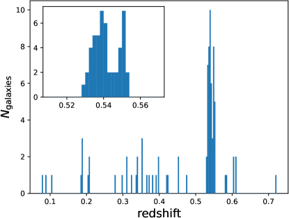
Figure 2: Redshift histogram, with inset showing the redshift interval around the cluster.

4.2 Subclustering and kinematics

First, we note that the redshift histogram shows no serious foreground or background cluster candidates that could complicate the interpretation of X-ray or lensing data in this field. We proceed to analyze the redshift window from 0.52–0.56, containing 49 galaxies. We estimate the mean redshift and velocity dispersion using the biweight estimator (Beers et al., 1990), with uncertainties obtained via the jackknife method. We find the systemic redshift to be $0.5410\pm 0.0012$ and the velocity dispersion to be $1398\pm 104\;$\mathrm{k}\mathrm{m}\;\mathrm{s}^{-1}$$, likely inflated by merger activity. The histogram suggests that the distribution may be bimodal, so we apply an Anderson-Darling (AD) test for consistency with a single Gaussian and find a p-value in the range (0.025,0.05), which is suggestive but not definitive.

Redshift bimodality? A natural explanation for two redshift peaks would be that the two subclusters have some relative velocity along the line of sight. To visualize any correlation between velocity and sky positions, we present a color-coded map in Figure 3. There is no apparent correlation between position and velocity, which agrees with the BCG redshifts (§1) in suggesting that the two subclusters have negligible relative line-of-sight velocity. This raises the question of whether the second redshift peak indicates a third body, or is a statistical fluke.

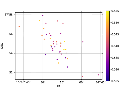
Figure 3: Map of galaxy redshifts in the range $0.52{<}z{<}0.56$. There is no apparent correlation between redshift and position, suggesting that any bimodality in the redshift histogram is not due to a radial velocity difference between the two subclusters.

To test this further, Figure 4 shows the relationship between galaxy redshift and position along the merger axis, with the NE (SW) subcluster defined as having positive (negative) position. The galaxy labeled C in Figure 1 appears at the origin in this coordinate system. There does appear to be a dearth of redshifts around $z=0.545$, but this dearth appears in both subclusters, and both subclusters have a similar fraction of galaxies with redshift greater than this. An Anderson-Darling test for consistency with a single Gaussian finds $p>0.15$ ($p=0.10$) for the NE (SW) subcluster. In other words, each subcluster is consistent with a single Gaussian but pooling their galaxies leads to stronger evidence for an additional velocity component. If this bimodality is real, it is difficult to explain with a physical model: the line-of-sight velocity difference between groups at $z{=}0.535$ and $z{=}0.55$ is about $2900\;$\mathrm{k}\mathrm{m}\;\mathrm{s}^{-1}$$ in the frame of the cluster, but the substantial projected separation between galaxy groups and the X-ray peak argues strongly against a line-of-sight merger. Hence, we tentatively attribute the dip in the redshift histogram (Figure 2) to the small spectroscopic sample size rather than a real physical feature.

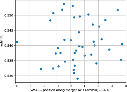
Figure 4: Galaxy redshift vs position along the merger axis. If there is redshift bimodality (with a possible dearth of galaxies around $z=0.545$), it cannot be assigned to either the NE or SW subcluster specifically.

Another tool relevant to this issue is the mc3gmm code (Golovich et al., 2019) which creates a Gaussian Mixture Model (GMM) for a given number of subclusters $n_{s}$. Each subcluster is represented by eight free parameters: central R.A., decl., and redshift; dispersion in the same three dimensions; covariance between R.A. and decl., to allow for elliptical clusters; and an amplitude representing the fraction of galaxies in that subcluster. The GMM likelihood is reported, which along with the number of free parameters can be used to compute a Bayesian Information Criterion (BIC) score to assess which model parameters are justified by the data. According to this tool, the entire system is best modeled by a single Gaussian. A second Gaussian, overlapping on the sky but at slightly higher redshift, is strongly disfavored. A model with two subclusters at the same redshift but separated on the sky is also disfavored. However, we note that this tool considers only the 49 spectroscopically confirmed member galaxies; it neglects the galaxy photometry and the X-ray evidence that two subclusters have passed through each other. We conclude that while 49 member velocities and positions are too few to justify a bimodal (or more complicated) model on their own, the totality of the evidence strongly favors a recent core passage between two halos. Furthermore, the spectroscopic survey has demonstrated that foreground/background structures may be neglected.

Manual subclustering. We return to using the position along the merger axis as visualized in Figure 4 to define the NE (SW) subcluster as those galaxies with positive (negative) coordinates, omitting BCG C which is difficult to assign to either subcluster. These two subclusters have consistent mean redshifts: $0.5416\pm 0.0014$ ($0.5398\pm 0.0022$) for NE (SW) based on 31 (17) members, with velocity dispersions of $1420\pm 122$ ($1356\pm 283$) $\mathrm{k}\mathrm{m}\;\mathrm{s}^{-1}$ respectively. The redshift difference between subclusters is $0.0018\pm 0.0026$, or $350\pm 507\;$\mathrm{k}\mathrm{m}\;\mathrm{s}^{-1}$$ in the frame of the cluster.

The subcluster velocity dispersions are quite high, even when compared to a sample of merging clusters such as that of Golovich et al. (2019). The nature of the putative second redshift peak must be resolved in order to properly interpret this high velocity dispersion. Note, however, that the velocity dispersion is a strong function of time in a merger, peaking around the time of pericenter (Pinkney et al., 1996; Takizawa et al., 2010). In §6 we present evidence that this merger is seen sooner after pericenter than most of the systems in Golovich et al. (2019).

5 Weak lensing analysis

Using archival HST/ACS F814W imaging (Proposal ID: 14098, PI: Ebeling), we perform a weak-lensing analysis of RMJ1508. The image was taken on 20 Feb 2016 with an exposure time of 1200 seconds. After standard instrumental signature removal, we used SExtractor (Bertin & Arnouts, 1996) to detect objects. For each galaxy, we generated a relevant PSF model following the method of Jee et al. (2007) by utilizing their publicly available PSF catalog. Each galaxy was fit with a PSF-convolved Gaussian model parametrized by a pre-PSF complex ellipticity; see Finner et al. (2017), Finner et al. (2021), and Finner et al. (2023) for more details on our ACS weak-lensing pipeline. In order to prevent spurious sources such as diffraction spikes around bright stars and poorly fit objects from entering the source catalog, we remove objects with ellipticity greater than 0.8, ellipticity uncertainty greater than 0.3, and intrinsic size (pre-psf) less than 0.5 pixels.

Next, we must filter out as many foreground and cluster galaxies as possible from our source catalog and, at the same time, minimize the loss of background sources. For this step, we use galaxy colors based on archival HST/ACS F606W imaging taken as part of the same program identified above; this image was taken on 27 August 2016 with an exposure time of 1200 seconds. The cluster red sequence follows a linear relation at an F606W-F814W color of approximately 1.2. We select background galaxies by keeping those with F606W-F814W color less than 1. In addition, we constrain the F814W magnitude to be fainter than 24. The final source catalog contains 28.2 galaxies arcmin^-2 (988 galaxies total). We apply the same color and magnitude cuts to the GOODS-S photometric redshift catalog (Dahlen et al., 2013) and find that the contamination by foreground galaxies is expected to be 6.5%; this is accounted for when fitting mass models below. Cluster galaxies may contribute additionally to the contamination. However, inspection of a 2-D source density map does not reveal any obvious associations with the known subclusters.

Before fitting mass models, we present a nonparametric reconstruction of the surface mass density (convergence) field using the FIATMAP code (Wittman et al., 2006), which convolves the observed shear field with a kernel of the form

$$r^{-2}(1-\exp({-r^{2}\over 2r_{i}^{2}}))\exp({-r^{2}\over 2r_{o}^{2}}),$$ (2)

where $r_{i}$ and $r_{o}$ are inner and outer cutoffs, respectively. Following Wittman et al. (2023), we used $r_{i}=50\;$\mathrm{a}\mathrm{r}\mathrm{c}\mathrm{s}\mathrm{e}\mathrm{c}$$ and $r_{o}=100\;$\mathrm{a}\mathrm{r}\mathrm{c}\mathrm{s}\mathrm{e}\mathrm{c}$$. The resulting mass map has 1.5 arcsec per pixel. Figure 5 shows this map as a set of contours overlaid on a Pan-STARRS multiband image (Waters et al., 2020). Each galaxy subcluster is associated with a weak lensing peak, with a trough in between. The well-defined SW lensing peak is offset to the southwest of the local X-ray peak, supporting the scenario in which this subcluster is traveling southwest, outbound after a recent pericenter passage in which ram pressure slowed the gas. The NE lensing peak is less well defined, such that the sign of its offset relative to its local X-ray peak cannot be determined.

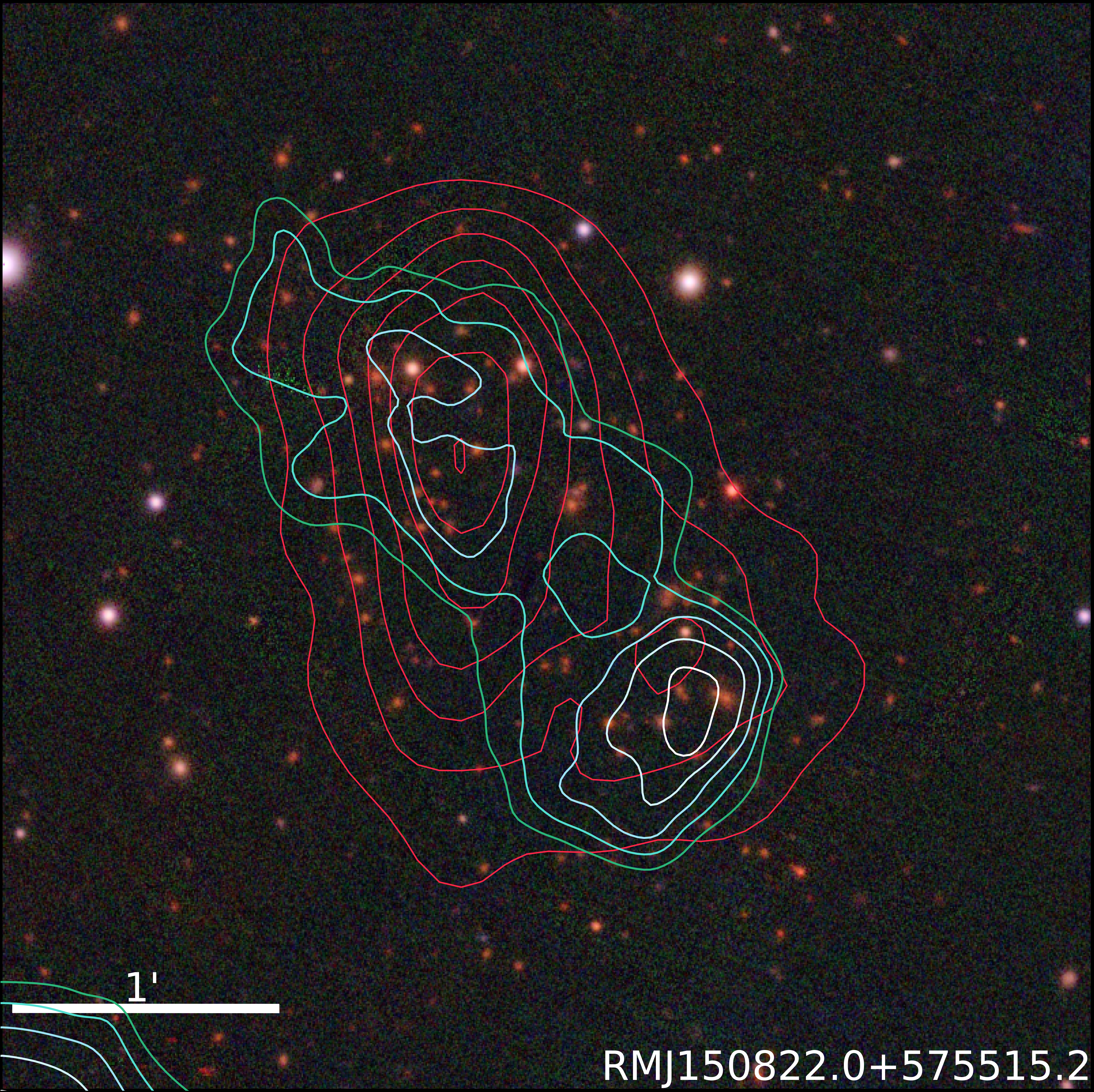
Figure 5: Pan-STARRS multiband (gri) image with surface mass density contours from weak lensing overlaid. The contour color map goes from green to blue to white in ascending order of mass density. (Note that the central closed contour indicates a trough rather than a peak). The red contours represent XMM-Newton surface brightness. The southwestern subcluster has a higher, more well-defined mass peak, whereas the northeastern subcluster’s mass peak is more irregular in shape. The X-ray surface brightness may be described as a NE-SW ridge with a main peak near the NE subcluster and a secondary peak near the SW subcluster, albeit lagging that subcluster if it is outbound.

We estimate the mass of each subcluster by fitting a two-halo NFW model with a mass-concentration relation from Child et al. (2018). We use the galsim library to compute the shear of the two-halo model at the position of each background galaxy, and we set the distance ratio $\beta$ of the sources to the mean distance ratio of sources in the GOODS-S sources photometric catalog (Dahlen et al., 2013) meeting the color and magnitude cuts described above ($\bar{\beta}=0.45$ where the bar indicates averaging over sources). Given a lens model, galsim predicts the reduced shear field $g(\beta)$ for a single source plane at distance ratio $\beta$. However, $g$ is a nonlinear function of $\beta$ such that $\overline{g(\beta)}\neq g(\bar{\beta})$. To correct for this, we use the Seitz & Schneider (1997) approximation

$$\overline{g(\beta)}\approx g(\bar{\beta})\left[1+(\frac{\overline{\beta^{2}}}{(\bar{\beta})^{2}}-1)\kappa\right]$$ (3)

noting that this correction is nontrivial only near the NFW peaks where the convergence $\kappa$ is not negligible.

We used scipy.optimize.least_squares to optimize six parameters: the mass and 2-D positions of each of the two NFW halos. We fixed the concentration of each halo to the value predicted by the Child et al. (2018) mass-concentration relation, after finding that the NE halo does not converge when allowing for scatter in this relation. We put broad, flat priors on each of the six parameters: 1–300$\times 10^{13}$ M_⊙ on the mass and $\pm 30^{\prime\prime}$ on the location of each halo. We find the SW (NE) mass to be $M_{\rm 200c}=36\pm 11\times 10^{13}$ ($38\pm 11\times 10^{13}$) M${}_{\odot}/h$; these uncertainties are found by bootstrap resampling the source catalog but are similar to those inferred from the curvature of the likelihood surface. The fitted positions are consistent with the convergence map peaks, regardless of starting position within the bounding box, with uncertainties of about $\pm 5^{\prime\prime}$. Note that Lee et al. (2023) recently found that for merging clusters seen shortly after pericenter, the WL-derived masses tend to be biased high, since the mass profile is disturbed by the merger and deviates from the fitted model profiles. The bias is a function of time since pericenter (TSP) and mass. For RMJ1508, at the most unfavorable TSP the bias would likely be between 23% and 41%.

Comparing the weak lensing masses with the mass suggested by the proxies listed in §2 is not straightforward given that the references cited there did not treat the system as composed of two clusters. Furthermore, various mass proxies are not expected to agree well in a merging system. Nevertheless, we note that the sum of the weak lensing masses is comparable to the proxy estimates. After accounting for $h^{-1}$ the sum of our weak lensing M_200c masses is $10.6\pm 2.2\times 10^{13}$ M_⊙, which is higher than but consistent with the $\approx 8$ one would get by converting the Planck and X-ray masses cited in §2 to M_200c, and lower than but consistent with the M_200c estimates from the mass-richness relation. (Note that the mass inferred from lensing would increase if one draws a larger virial radius based on the combined mass of the two halos in the lensing model, but it is not clear that this procedure provides a more rigorous comparison with the mass proxies.)

As a test of whether a six-parameter model (including mass and 2-D position parameters for each of the two halos) is justified, we compute the Bayesian Information Criterion (BIC). Compared to a model with no lens mass, the two-halo model has a BIC lower by $25$ logarithmic units, which is considered very strong evidence (Kass & Raftery, 1995). Compared to a model with a single halo in the SW, the two-halo model is again very strongly preferred ($\Delta\textrm{BIC}=17$).

We bootstrap-resample the catalog of source galaxies to estimate the uncertainty in the position of each mass peak. We generate 10,000 bootstrap realizations of the mass map and record the global peak position for each one. We then use the peak positions as the input to a k-means algorithm (sklearn.cluster.KMeans) with the number of clusters fixed at two. The k-means algorithm iteratively assigns each recorded peak to one of the two clusters and calculates the two centroid positions, minimizing the distance between data points and centroid within each group. After convergence is obtained, we find that the peak is located in the SW (NE) subcluster in 61% (39%) of the bootstrap realizations. By randomly sampling pairs of NE and SW peaks, we estimate the 68% confidence interval on the distance between peaks. We find that the NE and SW mass peaks are separated by $520^{+162}_{-125}$ kpc, with most of the uncertainty stemming from uncertainty in the position of the northern mass.

The bootstrap-resampling method can also be used to assess the detection significance of each peak. In order to do so, we estimate the noise level at each pixel in the mass map by computing the rms of the pixel value across all 10,000 realizations. We then divide the average mass map by the noise map in order to obtain a significance map. We find that the southwestern (northeastern) mass peak is detected at a significance level of $5.3\sigma$ ($4.7\sigma$).

6 Dynamical parameters via Simulated analogs

A technique recently developed by Wittman et al. (2018a) and Wittman (2019) uses observationally-derived parameters for a merger—such as subcluster mass and projected separation—to find analog systems in cosmological simulations. This allows for estimating important merger parameters that are not immediately available from observations—e.g. time since pericenter (TSP), pericenter distance, and maximum velocity—and reconstructing the merger scenario. The analogs could also form the basis for resimulating the merger process at higher resolution and with more physics.

We select dark matter halo pairs undergoing merging processes in the Big Multidark Planck (BigMDPL) Simulation (Klypin et al., 2016) and conduct mock observations by varying the viewing angle. For each analog, we compute its likelihood of matching the observed parameters of our cluster as a function of the viewing angle. The input parameters required to calculate the likelihoods are the projected separation $d_{\rm proj}$ between mass peaks, the line-of-sight relative velocity $\Delta v_{\rm los}$, and the masses of the two subclusters. The analog’s likelihood is then used as its weight when computing the derived dynamical parameters of the merger. For more details on the method, we refer to Wittman (2019).

In §5, we measured a projected separation of 520 kpc. Since the analog method takes symmetric error bars to calculate the likehoods, we use an uncertainty of $\pm 148$ kpc on this measurement, which represents a $\sim 70\%$ confidence interval. We also used $\Delta v_{\rm los}$ = $350\pm 507\;$\mathrm{k}\mathrm{m}\;\mathrm{s}^{-1}$$ from §4.2, as well as the subcluster masses estimated in §5 after accounting for our adopted value of $h$$:M_{\rm 200c}=5.2\pm 1.6\times 10^{14}$ M_⊙ and $M_{\rm 200c}=5.5\pm 1.6\times 10^{14}$ M_⊙ for the SW and NE subclusters, respectively.

The resulting $68\%$ and $95\%$ highest probability density confidence intervals of the inferred parameters are listed in Table 3. Our results suggest that RMJ1508 is a merger seen shortly after pericenter: the TSP is between 96 and 236 Myr at the $68\%$ confidence level. For comparison, both the lower and upper boundaries of this confidence interval are lower than that of all the 11 clusters in the sample considered by Wittman (2019). The maximum relative speed between the two subclusters ($v_{\rm max}$), however, is comparable to the median of their sample. The angle $\theta$ denotes the angle between the subcluster separation vector and the line of sight, i.e., $\theta=90^{\circ}$ is a merger entirely in the plane of sky. Our results indicate a small line-of-sight component and are consistent with a merger in the plane of the sky. The angle $\varphi$ is defined as the angle between the current separation and velocity vectors. When $\varphi<90^{\circ}$ ($>90^{\circ}$), the merger is in its outbound (returning) phase. Also, $\varphi=0$ would indicate a fully head-on collision and a negligible impact parameter. The inferred value of $\varphi$ for RMJ1508 suggests a collision that is largely head-on. The analogs are overwhelmingly in the outbound phase: the likelihood ratio of outbound to returning analogs is 384:1.

Table 3: Dynamical parameters from analogs

Confidence	TSP (Myr)	$v_{\rm max}$ ($\mathrm{k}\mathrm{m}\;\mathrm{s}^{-1}$)	$\theta$ (deg)	$\varphi$ (deg)
68%	96-236	2062-2656	62-90	4-26
95%	0-357	1601-2824	36-90	1-50

7 Radio observations and results

Extended radio emission from galaxy clusters in the form of radio relics and halos is often a valuable resource to help constrain the merger scenario. A recent attempt at identifying extended radio sources in RMJ1508 with data from the LOFAR Two-meter Sky Survey (LoTSS-DR2) yielded inconclusive results due to poor image quality in the cluster region (Botteon et al., 2022), encouraging new observations.

We were granted 15 hours on the upgraded GMRT (uGMRT, Gupta et al., 2017) for Band 4 (550-900 MHz) observations of this cluster (proposal code 42_069) with 4^′′ synthesized beam size. Observations were taken on 4 July and 19 July 2022. We used the SPAM pipeline (Intema, 2014) to calibrate the visibilities, and used wsclean (Offringa et al., 2014; Offringa & Smirnov, 2017) to create an image with a noise level of $50\text{\,}\mathrm{\SIUnitSymbolMicro}\mathrm{J}\mathrm{y}\;\mathrm{b}\mathrm{e}\mathrm{a}\mathrm{m}^{-1}$. We found no obvious extended emission in the cluster region.

Figure 6 shows the radio contours from the resulting image overlaid on the Pan-STARRS multiband image. A relatively bright point source can be seen in the southwestern subcluster, near the image center. Our spectroscopic data confirms the galaxy at the origin of this radio emission is at the cluster redshift. Of the five other fainter sources in the central cluster region, four are centered on galaxies we have spectroscopic redshifts for, all of which are also at the cluster redshift.

Figure 6: GMRT 650 MHz contours over Pan-STARRS multiband image. The first contour level is at $80\text{\,}\mathrm{\SIUnitSymbolMicro}\mathrm{J}\mathrm{y}\;\mathrm{b}\mathrm{e}\mathrm{a}\mathrm{m}^{-1}$, and subsequent contour levels are multiplied by a factor of 2.

8 Merger scenario

The X-ray morphology of RMJ1508 shows a projected separation between the two X-ray peaks in the plane of the sky of $411.6\pm 16.3$ kpc. This is a smaller projected separation than those measured between the two BCGs (697 kpc) and the two WL peaks ($\sim 500$ kpc). In the SW subcluster, the X-ray surface brightness exhibits a local peak that is removed from the corresponding BCG and WL-peak positions (see Figure 5), suggesting a dissociation between the ICM gas and dark matter. Assuming a post-pericenter, outgoing merger scenario, the gas of the SW subcluster lags behind the associated DM halo and BCG as the two subclusters move away from each other towards apocenter, due to the ram pressure resulting from the interaction with the other subcluster’s ICM. The NE X-ray peak, which presents a higher surface brightness than the SW peak, also lags behind its corresponding BCG, although the broader profile of the NE mass peak doesn’t allow for a definitive conclusion on the DM/ICM dissociation. The NE BCG exhibits strong-lensing features (see Figure 1), which could potentially be used to conduct a strong-lensing analysis and improve the constraints on the NE mass distribution. However, the redshift of the lensed galaxy remains unknown.

In order to describe the merger scenario, we define the merger axis as the line connecting the SW and NE centroids of the mass-peak positions, which are calculated from our 10,000 bootstrap realizations of the WL convergence maps (as explained in §5). We find the position angle of this axis to be 39^∘ east of north. We define the origin of our merger axis at the projected position of the galaxy labeled ”C” in Figure 1. The axis is shown in Figure 7, along with the positions of the BCGs, the X-ray peaks, and the WL peaks.

Figure 7: Definition of the merger axis (white solid line) using the centroids of the bootstrap-resampled WL peaks (cyan circles). The dashed line shows the perpendicular axis that passes through BCG-C, defining the origin of the coordinate system. The two BCGs are circled in yellow, and the X-ray surface brightness peaks are marked in magenta. The background image is Pan-STARRS multiband with overlaid X-ray contours.

The projected positions along the merger axis of the WL and X-ray peaks and of the BCG for each subcluster are shown in Figure 8. The violin plot displays the density along the merger axis of the WL mass map peaks for the 10,000 bootstrap realizations. Note that both the mass map in Figure 5 and the bootstrap-resampled WL peak distribution shown in Figure 8 present a bimodal shape in the NE subcluster. For more than half of the bootstrap realizations, the NE WL peak is actually closer to the origin of the merger axis than the X-ray peak, which contradicts the expectation for a merger seen shortly after pericenter. This raises the question of whether the NE dark matter halo really possesses non-trivial substructure, or if this feature is an artifact of the limited sample of background galaxies. The answer possibly requires deeper imaging covering a larger field-of-view.

Figure 8: Subcluster components along the merger axis. The orange markers show the X-ray peaks, and the magenta stars show the BCG positions. The violin plot represents the density of bootstrap-resampled WL mass map peaks. The centroid of the WL peak distribution for each subcluster (blue circles) is computed by the k-means algorithm with two components. The error bars for the X-ray peak positions were estimated by fitting two Gaussians to the projected surface brightness profile along the merger axis and finding the uncertainty in the fitted positions.

The distances along the merger axis between all three measured components of each subcluster are listed in Table 4. For the SW subcluster, the projected separation between WL and X-ray peaks is larger than the error bars, suggesting that the peak of the DM distribution is located to the south of the gas density peak. Although there is a $~{}30\;$\mathrm{k}\mathrm{p}\mathrm{c}$$ distance between the projected positions of the mass peak and the BCG, this distance is well within the limits of the WL uncertainty. For the NE subcluster, the X-ray peak is located $\sim 180\;$\mathrm{k}\mathrm{p}\mathrm{c}$$ to the southwest of the BCG. However, the previously discussed morphology of the NE mass profile results in large uncertainties in the position of its peak along the merger axis, prohibiting a clear determination of the relative positions between WL and X-ray peaks, as well as WL peak and BCG.

Table 4: Distance Along Merger Axis (kpc)

	NE	SW
WL – BCG	$-144.7^{+147.6}_{-92.6}$	$26.7^{+60.2}_{-50.4}$
X-ray – BCG	$-182.0\pm 6.9$	$106.6\pm 14.7$
WL – X-ray	$37.3^{+147.8}_{-92.9}$	$-79.9^{+61.9}_{-52.5}$

9 Summary

Our multiwavelength analysis shows that RMJ1508 is a cluster in a merging state seen shortly after first pericenter passage. By fitting a two-halo NFW model to the WL mass maps, we infer that the two subclusters have approximately the same mass. The NE subcluster, however, has a broader mass peak than the SW, which is more well-defined. The X-ray morphology, revealed by XMM-Newton archival data, exhibits two surface brightness peaks between the subclusters’ BCGs, in a classic dissociative merger configuration.

Our spectroscopy results reveal that the line-of-sight component of the relative velocities between the two subclusters is small, suggesting a merger very close to the plane of the sky. By selecting analog systems in cosmological simulations, we confirm that the merging axis is $\leq 28^{\circ}$ from the plane of the sky at the $68\%$ confidence level. The analogs also indicate a time since pericenter ranging from 96 to 236 Myr.

In summary, the system we have presented possesses many features that make it a great candidate for further study. The two equal-mass subclusters are colliding head-on, resulting in dissociation between DM and ICM components, especially in the SW subcluster. The merger axis is conveniently placed near the plane of the sky, and the cluster’s simple, binary nature makes the merger scenario relatively easy to identify and model.

Follow-up observations of RMJ1508 could improve our understanding of the system. For example, ground-based imaging suitable for weak lensing analysis could help improve the accuracy of the mass maps and either confirm or rule out the substructure observed in the NE mass peak. In addition, the observed merger parameters could be used to stage high-resolution hydro simulations and leverage the system’s suitability to test dark matter models, potentially improving the constraints on the dark matter self-interaction cross-section. Moreover, our merger-finding method, which enabled the discovery of this cluster, is well suited to take advantage of the upcoming optical and X-ray surveys such as the Legacy Survey of Space and Time (LSST; Ivezic et al. (2008)) and e-ROSITA, and has the potential to significantly expand the ensemble of binary, dissociative merging clusters that can help uncover new physics.

References

- Ahumada et al. (2020) Ahumada, R., Allende Prieto, C., Almeida, A., et al. 2020, ApJS, 249, 3, doi: 10.3847/1538-4365/ab929e
- Arnaud (1996) Arnaud, K. A. 1996, in Astronomical Society of the Pacific Conference Series, Vol. 101, Astronomical Data Analysis Software and Systems V, ed. G. H. Jacoby & J. Barnes, 17
- Arnaud et al. (2002) Arnaud, M., Majerowicz, S., Lumb, D., et al. 2002, Astronomy & Astrophysics, 390, 27, doi: 10.1051/0004-6361:20020669
- Bartalucci et al. (2019) Bartalucci, I., Arnaud, M., Pratt, G. W., Démoclès, J., & Lovisari, L. 2019, A&A, 628, A86, doi: 10.1051/0004-6361/201935984
- Beck et al. (2021) Beck, R., Szapudi, I., Flewelling, H., et al. 2021, MNRAS, 500, 1633, doi: 10.1093/mnras/staa2587
- Beers et al. (1990) Beers, T. C., Flynn, K., & Gebhardt, K. 1990, AJ, 100, 32, doi: 10.1086/115487
- Bertin & Arnouts (1996) Bertin, E., & Arnouts, S. 1996, A&AS, 117, 393, doi: 10.1051/aas:1996164
- Botteon et al. (2020) Botteon, A., Brunetti, G., Ryu, D., & Roh, S. 2020, A&A, 634, A64, doi: 10.1051/0004-6361/201936216
- Botteon et al. (2022) Botteon, A., Shimwell, T. W., Cassano, R., et al. 2022, A&A, 660, A78, doi: 10.1051/0004-6361/202143020
- Bradač et al. (2006) Bradač, M., Clowe, D., Gonzalez, A. H., et al. 2006, ApJ, 652, 937, doi: 10.1086/508601
- Brodwin et al. (2013) Brodwin, M., Stanford, S. A., Gonzalez, A. H., et al. 2013, ApJ, 779, 138, doi: 10.1088/0004-637X/779/2/138
- Carter & Read (2007) Carter, J. A., & Read, A. M. 2007, Astronomy & Astrophysics, 464, 1155, doi: 10.1051/0004-6361:20065882
- Child et al. (2018) Child, H. L., Habib, S., Heitmann, K., et al. 2018, ApJ, 859, 55, doi: 10.3847/1538-4357/aabf95
- Clowe et al. (2006) Clowe, D., Bradač, M., Gonzalez, A. H., et al. 2006, ApJ, 648, L109, doi: 10.1086/508162
- Dahlen et al. (2013) Dahlen, T., Mobasher, B., Faber, S. M., et al. 2013, ApJ, 775, 93, doi: 10.1088/0004-637X/775/2/93
- Dawson et al. (2012) Dawson, W. A., Wittman, D., Jee, M. J., et al. 2012, ApJ, 747, L42, doi: 10.1088/2041-8205/747/2/L42
- De Luca & Molendi (2004) De Luca, A., & Molendi, S. 2004, A&A, 419, 837, doi: 10.1051/0004-6361:20034421
- Faber et al. (2003) Faber, S. M., Phillips, A. C., Kibrick, R. I., et al. 2003, in Society of Photo-Optical Instrumentation Engineers (SPIE) Conference Series, Vol. 4841, Instrument Design and Performance for Optical/Infrared Ground-based Telescopes, ed. M. Iye & A. F. M. Moorwood, 1657–1669
- Finner et al. (2017) Finner, K., Jee, M. J., Golovich, N., et al. 2017, ApJ, 851, 46, doi: 10.3847/1538-4357/aa998c
- Finner et al. (2021) Finner, K., HyeongHan, K., Jee, M. J., et al. 2021, ApJ, 918, 72, doi: 10.3847/1538-4357/ac0d00
- Finner et al. (2023) Finner, K., Randall, S. W., Jee, M. J., et al. 2023, ApJ, 942, 23, doi: 10.3847/1538-4357/ac9fd3
- Gabriel et al. (2004) Gabriel, C., Denby, M., Fyfe, D. J., et al. 2004, in Astronomical Society of the Pacific Conference Series, Vol. 314, Astronomical Data Analysis Software and Systems (ADASS) XIII, ed. F. Ochsenbein, M. G. Allen, & D. Egret, 759
- Ghizzardi et al. (2010) Ghizzardi, S., Rossetti, M., & Molendi, S. 2010, A&A, 516, A32, doi: 10.1051/0004-6361/200912496
- Golovich et al. (2019) Golovich, N., Dawson, W. A., Wittman, D. M., et al. 2019, ApJ, 882, 69, doi: 10.3847/1538-4357/ab2f90
- Gupta et al. (2017) Gupta, Y., Ajithkumar, B., Kale, H. S., et al. 2017, Current Science, 113, 707, doi: 10.18520/cs/v113/i04/707-714
- Harvey et al. (2015) Harvey, D., Massey, R., Kitching, T., Taylor, A., & Tittley, E. 2015, Science, 347, 1462, doi: 10.1126/science.1261381
- Intema (2014) Intema, H. T. 2014, SPAM: Source Peeling and Atmospheric Modeling, Astrophysics Source Code Library, record ascl:1408.006. http://ascl.net/1408.006
- Ivezic et al. (2008) Ivezic, Z., Tyson, J. A., Allsman, R., et al. 2008, ArXiv e-prints. https://arxiv.org/abs/0805.2366
- Jee et al. (2007) Jee, M. J., Blakeslee, J. P., Sirianni, M., et al. 2007, PASP, 119, 1403, doi: 10.1086/524849
- Kang (2021) Kang, H. 2021, Journal of Korean Astronomical Society, 54, 103, doi: 10.48550/arXiv.2106.08521
- Kaplinghat et al. (2016) Kaplinghat, M., Tulin, S., & Yu, H.-B. 2016, Phys. Rev. Lett., 116, 041302, doi: 10.1103/PhysRevLett.116.041302
- Kass & Raftery (1995) Kass, R. E., & Raftery, A. E. 1995, Journal of the American Statistical Association, 90, 773, doi: 10.1080/01621459.1995.10476572
- Kim et al. (2017) Kim, S. Y., Peter, A. H. G., & Wittman, D. 2017, MNRAS, 469, 1414, doi: 10.1093/mnras/stx896
- Klypin et al. (2016) Klypin, A., Yepes, G., Gottlöber, S., Prada, F., & Heß, S. 2016, MNRAS, 457, 4340, doi: 10.1093/mnras/stw248
- Lee et al. (2023) Lee, W., Cha, S., Jee, M. J., et al. 2023, ApJ, 945, 71, doi: 10.3847/1538-4357/acb76b
- Mansheim et al. (2017) Mansheim, A. S., Lemaux, B. C., Tomczak, A. R., et al. 2017, MNRAS, 469, L20, doi: 10.1093/mnrasl/slx041
- Markevitch et al. (2004) Markevitch, M., Gonzalez, A. H., Clowe, D., et al. 2004, ApJ, 606, 819, doi: 10.1086/383178
- Markevitch & Vikhlinin (2007) Markevitch, M., & Vikhlinin, A. 2007, Phys. Rep., 443, 1, doi: 10.1016/j.physrep.2007.01.001
- Miller & Owen (2003) Miller, N. A., & Owen, F. N. 2003, AJ, 125, 2427, doi: 10.1086/374767
- Moravec et al. (2020) Moravec, E., Gonzalez, A. H., Dicker, S., et al. 2020, ApJ, 898, 145, doi: 10.3847/1538-4357/aba0b2
- Nagai et al. (2013) Nagai, D., Lau, E. T., Avestruz, C., Nelson, K., & Rudd, D. H. 2013, ApJ, 777, 137, doi: 10.1088/0004-637X/777/2/137
- Newman et al. (2013) Newman, J. A., Cooper, M. C., Davis, M., et al. 2013, ApJS, 208, 5, doi: 10.1088/0067-0049/208/1/5
- Offringa et al. (2014) Offringa, A. R., McKinley, B., Hurley-Walker, et al. 2014, MNRAS, 444, 606, doi: 10.1093/mnras/stu1368
- Offringa & Smirnov (2017) Offringa, A. R., & Smirnov, O. 2017, MNRAS, 471, 301, doi: 10.1093/mnras/stx1547
- Pinkney et al. (1996) Pinkney, J., Roettiger, K., Burns, J. O., & Bird, C. M. 1996, ApJS, 104, 1, doi: 10.1086/192290
- Planck Collaboration et al. (2016) Planck Collaboration, Ade, P. A. R., Aghanim, N., et al. 2016, A&A, 594, A27, doi: 10.1051/0004-6361/201525823
- Pratt et al. (2022) Pratt, G. W., Arnaud, M., Maughan, B. J., & Melin, J. B. 2022, A&A, 665, A24, doi: 10.1051/0004-6361/202243074
- Prochaska et al. (2020) Prochaska, J. X., Hennawi, J. F., Westfall, K. B., et al. 2020, Journal of Open Source Software, 5, 2308, doi: 10.21105/joss.02308
- Prochaska et al. (2020) Prochaska, J. X., Hennawi, J., Cooke, R., et al. 2020, pypeit/PypeIt: Release 1.0.0, v1.0.0, Zenodo, doi: 10.5281/zenodo.3743493
- Randall et al. (2008) Randall, S. W., Markevitch, M., Clowe, D., Gonzalez, A. H., & Bradač, M. 2008, ApJ, 679, 1173, doi: 10.1086/587859
- Robertson et al. (2017) Robertson, A., Massey, R., & Eke, V. 2017, MNRAS, 465, 569, doi: 10.1093/mnras/stw2670
- Rozo & Rykoff (2014) Rozo, E., & Rykoff, E. S. 2014, ApJ, 783, 80, doi: 10.1088/0004-637X/783/2/80
- Rykoff et al. (2014) Rykoff, E. S., Rozo, E., Busha, M. T., et al. 2014, ApJ, 785, 104, doi: 10.1088/0004-637X/785/2/104
- Sagunski et al. (2021) Sagunski, L., Gad-Nasr, S., Colquhoun, B., Robertson, A., & Tulin, S. 2021, J. Cosmology Astropart. Phys, 2021, 024, doi: 10.1088/1475-7516/2021/01/024
- Seitz & Schneider (1997) Seitz, C., & Schneider, P. 1997, A&A, 318, 687
- Sereno & Ettori (2017) Sereno, M., & Ettori, S. 2017, MNRAS, 468, 3322, doi: 10.1093/mnras/stx576
- Simet et al. (2017) Simet, M., McClintock, T., Mandelbaum, R., et al. 2017, MNRAS, 466, 3103, doi: 10.1093/mnras/stw3250
- Snowden & Kuntz (2014) Snowden, S. L., & Kuntz, K. D. 2014, XMM ESAS Cookbook. https://heasarc.gsfc.nasa.gov/docs/xmm/esas/cookbook/xmm-esas.html
- Sobral et al. (2015) Sobral, D., Stroe, A., Dawson, W. A., et al. 2015, MNRAS, 450, 630, doi: 10.1093/mnras/stv521
- Takizawa et al. (2010) Takizawa, M., Nagino, R., & Matsushita, K. 2010, PASJ, 62, 951, doi: 10.1093/pasj/62.4.951
- Tarrío et al. (2019) Tarrío, P., Melin, J. B., & Arnaud, M. 2019, A&A, 626, A7, doi: 10.1051/0004-6361/201834979
- van Weeren et al. (2019) van Weeren, R. J., de Gasperin, F., Akamatsu, H., et al. 2019, Space Sci. Rev., 215, 16, doi: 10.1007/s11214-019-0584-z
- van Weeren et al. (2016) van Weeren, R. J., Brunetti, G., Brüggen, M., et al. 2016, ApJ, 818, 204, doi: 10.3847/0004-637X/818/2/204
- van Weeren et al. (2017) van Weeren, R. J., Andrade-Santos, F., Dawson, W. A., et al. 2017, Nature Astronomy, 1, 0005, doi: 10.1038/s41550-016-0005
- Vazza & Brüggen (2014) Vazza, F., & Brüggen, M. 2014, MNRAS, 437, 2291, doi: 10.1093/mnras/stt2042
- Waters et al. (2020) Waters, C. Z., Magnier, E. A., Price, P. A., et al. 2020, ApJS, 251, 4, doi: 10.3847/1538-4365/abb82b
- Wen & Han (2015) Wen, Z. L., & Han, J. L. 2015, ApJ, 807, 178, doi: 10.1088/0004-637X/807/2/178
- Wen et al. (2009) Wen, Z. L., Han, J. L., & Liu, F. S. 2009, ApJS, 183, 197, doi: 10.1088/0067-0049/183/2/197
- Wen et al. (2012) —. 2012, ApJS, 199, 34, doi: 10.1088/0067-0049/199/2/34
- Wittman (2019) Wittman, D. 2019, ApJ, 881, 121, doi: 10.3847/1538-4357/ab3052
- Wittman et al. (2018a) Wittman, D., Cornell, B. H., & Nguyen, J. 2018a, ApJ, 862, 160, doi: 10.3847/1538-4357/aacf3e
- Wittman et al. (2006) Wittman, D., Dell’Antonio, I. P., Hughes, J. P., et al. 2006, ApJ, 643, 128, doi: 10.1086/502621
- Wittman et al. (2018b) Wittman, D., Golovich, N., & Dawson, W. A. 2018b, ApJ, 869, 104, doi: 10.3847/1538-4357/aaee77
- Wittman et al. (2023) Wittman, D., Stancioli, R., Finner, K., et al. 2023, arXiv e-prints, arXiv:2306.01715, doi: 10.48550/arXiv.2306.01715
- Yuan et al. (2022) Yuan, Z. S., Han, J. L., & Wen, Z. L. 2022, MNRAS, 513, 3013, doi: 10.1093/mnras/stac1037
- Zhang et al. (2023) Zhang, X., Simionescu, A., Gastaldello, F., et al. 2023, A&A, 672, A42, doi: 10.1051/0004-6361/202244761