Exploring Transformer Extrapolation

Abstract

Length extrapolation has attracted considerable attention recently since it allows transformers to be tested on longer sequences than those used in training. Previous research has shown that this property can be attained by using carefully designed Relative Positional Encodings (RPEs). While these methods perform well on a variety of corpora, the conditions for length extrapolation have yet to be investigated. This paper attempts to determine what types of RPEs allow for length extrapolation through a thorough mathematical and empirical analysis. We discover that a transformer is certain to possess this property as long as the series that corresponds to the RPE’s exponential converges. Two practices are derived from the conditions and examined in language modeling tasks on a variety of corpora. As a bonus from the conditions, we derive a new Theoretical Receptive Field (TRF) to measure the receptive field of RPEs without taking any training steps. Extensive experiments are conducted on the Wikitext-103, Books, Github, and WikiBook datasets to demonstrate the viability of our discovered conditions. We also compare TRF to Empirical Receptive Field (ERF) across different models, showing consistently matched trends on these datasets.

Introduction

Transformer (Vaswani et al. 2017) is advancing steadily in the areas of natural language processing (Qin et al. 2023b; Devlin et al. 2019; Liu et al. 2019; Qin et al. 2022b, a; Liu et al. 2022; Qin and Zhong 2023), computer vision (Dosovitskiy et al. 2020; Sun et al. 2022b; Lu et al. 2022; Hao et al. 2024), and audio processing (Gong, Chung, and Glass 2021; Akbari et al. 2021; Gulati et al. 2020; Sun et al. 2022a). Although it outperforms other architectures such as RNNs (Cho et al. 2014; Qin, Yang, and Zhong 2023) and CNNs (Kim 2014; Hershey et al. 2016; Gehring et al. 2017) in many sequence modeling tasks, its lack of length extrapolation capability limits its ability to handle a wide range of sequence lengths, i.e., inference sequences need to be equal to or shorter than training sequences. Increasing the training sequence length is only a temporary solution because the space-time complexity grows quadratically with the sequence length. Another option is to extend the inference sequence length by converting the trained full attention blocks to sliding window attention blocks (Beltagy, Peters, and Cohan 2020), but this will result in significantly worse efficiency than the full attention speed (Press, Smith, and Lewis 2022). How to permanently resolve this issue without incurring additional costs has emerged as a new topic.

A mainstream solution for length extrapolation is to design a Relative Positional Encoding (RPE) (Qin et al. 2023c) that concentrates attention on neighboring tokens. For example, ALiBi (Press, Smith, and Lewis 2022) applies linear decay biases to the attention to reduce the contribution from distant tokens. Kerple (Chi et al. 2022) investigates shift-invariant conditionally positive definite kernels in RPEs and proposes a collection of kernels that promote the length extrapolation property. It also shows that ALiBi is one of its instances. Sandwich (Chi, Fan, and Rudnicky 2022) proposes a hypothesis to explain the secret behind ALiBi and empirically proves it by integrating the hypothesis into sinusoidal positional embeddings.

In order to investigate transformer extrapolation, we first establish a hypothesis regarding why existing RPE-based length extrapolation methods (Qin et al. 2023a) have this capacity to extrapolate sequences in inference based on empirical analysis. Then we identify the conditions of RPEs that satisfy the hypothesis through mathematical analysis. Finally, the discovered conditions are empirically validated on a variety of corpora. Specifically, we assume that due to decay biases, existing RPE-based length extrapolation methods behave similarly to sliding window attention, i.e., only tokens within a certain range can influence the attention scores. A transformer can extrapolate for certain in this scenario since the out-of-range tokens have no effect on the attention outcomes. We derive that a transformer is guaranteed to satisfy this hypothesis if the series corresponding to the exponential of its RPE converges. Based on the observation, we show that previous RPE-based methods (Press, Smith, and Lewis 2022; Chi et al. 2022) can be seen as particular instances under the conditions. Two new practices from the conditions are derived and evaluated in language modeling.

The observed conditions not only shed light on the secret of length extrapolation but also offer a new perspective on computing the Theoretical Receptive Fields (TRF) of RPEs. In contrast to prior approaches that require training gradients to compute TRF, we propose a new way to calculate TRF that is solely based on the formulation of RPEs. Extensive experiments on Wikitext-103 (Merity et al. 2016), Books (Zhu et al. 2015), Github (Gao et al. 2020), and WikiBook (Wettig et al. 2022) validate the conditions. TRF calculated by our method substantially matches the trend of the Empirical Receptive Field (ERF) in real-world scenarios.

Preliminary

Before embarking on the journey of exploring, we introduce several preliminary concepts that will be used throughout the paper, such as softmax attention, relative positional encoding, length extrapolation, and sliding window attention. We also provide the necessary notations for the subsequent analysis, i.e., we use $\mathbf{M}$ to denote a matrix and $\mathbf{m}_{i}^{\top}$ to represent the $i$th row of $\mathbf{M}$. The complete math notations can be found in Appendix. Following previous work (Press, Smith, and Lewis 2022), we restrict our analysis to causal language models and assume that the max sequence length during training is $m$.

Softmax attention

Softmax attention is a key component of transformers which operates on query $\mathbf{Q}$, key $\mathbf{K}$ and value $\mathbf{V}$ matrices. Each matrix is a linear map that takes $\mathbf{X}\in\mathbb{R}^{n\times d}$ as input:

$$\mathbf{Q}=\mathbf{X}\mathbf{W}_{Q},\ \mathbf{K}=\mathbf{X}\mathbf{W}_{K},\ \mathbf{V}=\mathbf{X}\mathbf{W}_{V}\in\mathbb{R}^{n\times d},$$ (1)

where $n$ is the sequence length and $d$ is the dimension of the hidden feature. The output attention matrix $\mathbf{O}\in\mathbb{R}^{n\times d}$ can be formulated as:

$$\mathbf{O}=\mathrm{Softmax}(\mathbf{Q}\mathbf{K}^{\mkern-1.5mu\mathsf{T}}/\sqrt{d})\mathbf{V}.$$ (2)

To prevent information leakage in causal language modeling, a mask matrix $\mathbf{M}\in\mathbb{R}^{n\times n}$ is used to ensure that current tokens can only see previous tokens and themselves. The lower triangular elements of $\mathbf{M}$ are $0$, and the upper triangular ones, except for the diagonal, are $-\infty$. Then the output attention matrix $\mathbf{O}$ for causal language models will be:

$$\mathbf{O}=\mathrm{Softmax}(\mathbf{Q}\mathbf{K}^{\top}/\sqrt{d}+\mathbf{M})\mathbf{V}.$$ (3)

Note that Eq. 3 can be seen as a general form of attention, i.e., when the elements of $\mathbf{M}$ are all 0, Eq. 3 is degenerated to Eq. 2. For ease of discussion, we use Eq. 3 to represent attention computation.

Relative positional encoding

Positional encoding is designed to inject positional bias into transformers. Absolute Positional Encoding (APE) (Vaswani et al. 2017; Gehring et al. 2017) and Relative Positional Encoding (RPE) (Su et al. 2021; Liutkus et al. 2021; Press, Smith, and Lewis 2022; Chi et al. 2022) are the two most common types of positional encoding. In this paper, we focus on RPE because it is the key for length extrapolation, as shown in (Press, Smith, and Lewis 2022). An attention with RPE can be written as:

$$\mathbf{O}=\mathrm{Softmax}(\mathbf{Q}\mathbf{K}^{\top}/\sqrt{d}+\mathbf{M}+\mathbf{P})\mathbf{V},$$ (4)

where $\mathbf{P}\in\mathbb{R}^{n\times n}$ is a Toeplitz matrix that encodes relative positional information, i.e., $p_{ij}=p_{i-j}$. It is worth noting that $\mathbf{M}$ and $\mathbf{P}$ can be merged, and the merged matrix is still a Toeplitz matrix. We use $\mathbf{R}$ to represent the merged matrix and rewrite Eq. 4 as:

$$\mathbf{O}=\mathrm{Softmax}(\mathbf{Q}\mathbf{K}^{\top}/\sqrt{d}+\mathbf{R})\mathbf{V}.$$ (5)

Definition of length extrapolation

The property of length extrapolation allows a model to be tested on longer sequences than those used in training. Previous sequence modeling structures such as RNNs (Hochreiter and Schmidhuber 1997) and CNNs (Gehring et al. 2017) often naturally possess this property, but it is a difficult task for transformers. This property is only present in sliding window transformers and a few transformer variants with specifically designed RPEs (Chi et al. 2022; Press, Smith, and Lewis 2022; Chi, Fan, and Rudnicky 2022).

In language modeling, one token can only see itself and previous tokens. Therefore, regardless the sequence length, the performance should be stable for the neighboring tokens that are within the training sequence length (Beltagy, Peters, and Cohan 2020). For the tokens that are out of range, the performance will degrade if the model does not support length extrapolation (Press, Smith, and Lewis 2022). Based on the observation above, we give a definition of length extrapolation:

Definition 0.1.

For a language model $\mathcal{F}$, given dataset $\mathcal{X}$, if for any $n$, there is,

$$|ppl_{n}(\mathcal{X},\mathcal{F})-ppl_{m}(\mathcal{X},\mathcal{F})|/ppl_{m}(\mathcal{X},\mathcal{F})<\delta,$$ (6)

then $\mathcal{F}$ is considered to have the extrapolation property.

Here $\delta>0$ is a small constant, $ppl_{n}(\mathcal{X},\mathcal{F})$ means that $\mathcal{F}$ calculates perplexity with a max sequence length of $n$ on the data set $\mathcal{X}$. Empirically, if $|ppl_{n}(\mathcal{X},\mathcal{F})-ppl_{m}(\mathcal{X},\mathcal{F})|/ppl_{m}(\mathcal{X},\mathcal{F})$ becomes very large($\gg 1$) as $n$ increases, we consider that $\mathcal{F}$ does not have extrapolation property.

Sliding window attention

For the convenience of subsequent discussions, we define a window attention at position $i$ and window size $j$ as follows:

$$\mathbf{o}_{i}^{j} =\frac{\sum_{i-j+1\leq s\leq i}\exp(\mathbf{q}_{i}^{\top}\mathbf{k}_{s}/\sqrt{d})\exp(r_{is})\mathbf{v}_{s}}{\sum_{i-j+1\leq t\leq i}\exp(\mathbf{q}_{i}^{\top}\mathbf{k}_{t}/\sqrt{d})\exp(r_{it})}$$ (7)

$$\triangleq\frac{\sum_{i-j+1\leq s\leq i}c_{is}\mathbf{v}_{s}}{C_{ij}},$$

where $C_{ij}=\sum_{i-j+1\leq t\leq i}c_{it},c_{ij}=a_{ij}b_{ij},a_{ij}=\exp(\mathbf{q}_{i}^{\top}\mathbf{k}_{j}/\sqrt{d}),b_{ij}=\exp(r_{ij}),j\leq i.$

We further assume $\|\mathbf{x}_{i}\|\leq l,\mathbf{x}\in\{\mathbf{q},\mathbf{k},\mathbf{v}\}$, where $l>0$ is a constant. The $\mathbf{o}_{i}^{j}$ represents the attention output of the $i$-th token, which interacts with the $j$ tokens preceding it. Note that window attention naturally possesses the length extrapolation ability.

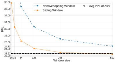
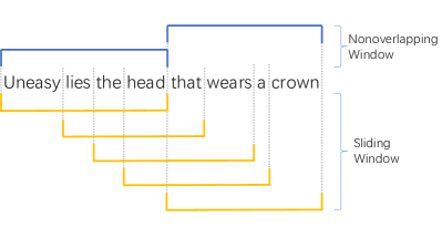
Figure 1: Sliding window inference vs Nonoverlapping inference. We illustrate the difference between sliding window inference and nonoverlapping inference in the right figure. The left figure shows the curves of ”Sliding Window“ and ”Nonoverlapping Window“corresponding to the ppls calculated by a language model at different inference window sizes. As a reference, we also plot the average ppl of Alibi extrapolated from 512 to 9216. The sliding window inference has much lower ppl than the nonoverlapping one and is close to the Alibi’s performance.

Table 1: Relative average inference time. We compute the relative average inference time of sliding window inference and nonoverlapping inference over a set of window sizes {16,32,64,128,258,512}. We also include the Alibi inference time as a reference.

Method	Rel Avg infer time
Sliding Window	44.35
Nonoverlapping Window	1.00
Alibi	1.00

There are two ways to infer window attention: nonoverlapping inference and sliding window inference as shown on the right of Figure 1. In sliding window inference, the tokens within each sliding window must be re-encoded multiple times, making it substantially slower than the nonoverlapping one. In table 1 we compare the average inference time over a group of window sizes between the sliding window inference and nonoverlapping window inference. The sliding window one is more than 44 times slower than the nonoverlapping one. However, as shown on the left of Figure 1, the sliding window inference has much lower ppl than the nonoverlapping one.

Transformer Extrapolation Exploration

In this section, we first describe the hypothesis about why existing RPE-based length extrapolation methods can extrapolate sequences in inference and provide empirical evidence for it. Then we derive the conditions for length extrapolation in detail and demonstrate that recent RPE-based length extrapolation methods (Chi et al. 2022; Press, Smith, and Lewis 2022) satisfy the conditions.

(a) Sliding window	(b)Sliding Window

Figure 2: Visualization of attention reweighting. We plot the reweighting schema of sliding window attention and Alibi linear decay bias. They share a similar behavior in that only neighboring tokens can influence the attention results.

The hypothesis

A sliding window attention with window size $w$ is equivalent to the following RPE on full attention:

$$\mathrm{m}_{ij}=\begin{cases}0,&i-j\leq w.\\ -\infty,&\mathrm{others}.\end{cases}$$ (8)

By comparing Eq. 8 and the corresponding RPE of Alibi (Press, Smith, and Lewis 2022) in Figure 2, we can see that they both have the same behavior in that they both concentrate tokens inside a specified range. Also, in Figure 1, we show that the performance of Alibi is similar to the sliding window attention when the window size is sufficiently large. Based on these two observations, we make the following hypothesis:

Hypothesis 0.1.

A RPE that makes a transformer extrapolatable needs to have similar behavior to sliding window attention, i.e., $\delta(i,j)$ should satisfy:

$$\forall\epsilon>0,\exists j_{0},s.t,j>j_{0},\delta(i,j)<\epsilon,$$ (9)

where $\delta(i,j)\triangleq\|\mathbf{o}_{i}^{i}-\mathbf{o}_{i}^{j}\|$, and the window length $j$ needs to be sufficiently large.

In the following sections, we will derive the conditions for RPEs that satisfy Eq. 9.

The conditions

Let us introduce the first lemma:

Lemma 0.2.

When the following condition is satisfied, Eq. 9 holds.

$${\lim}_{i\to\infty}C_{ii}\triangleq C<\infty.$$ (10)

Proof.

When $i\leq m$, the test sequence length is smaller than the max sequence length $m$ during training, take $j=i$, we get $\|\mathbf{o}_{i}^{i}-\mathbf{o}_{i}^{j}\|=\|\mathbf{o}_{i}^{i}-\mathbf{o}_{i}^{i}\|=0.$ When $i>m$, we can reformulate Eq. 7 as:

$$\mathbf{o}_{i}^{i} =\frac{\sum_{i-j+1\leq s\leq i}c_{is}\mathbf{v}_{s}+\sum_{1\leq s\leq i-j}c_{is}\mathbf{v}_{s}}{C_{ii}}$$

$$=\frac{\sum_{i-j+1\leq s\leq i}c_{is}\mathbf{v}_{s}}{C_{ij}}\frac{{C_{ij}}}{{C_{ii}}}+\frac{\sum_{1\leq s\leq i-j}c_{is}\mathbf{v}_{s}}{C_{ii}-C_{ij}}\frac{C_{ii}-C_{ij}}{C_{ii}}$$

$$=\frac{\sum_{i-j+1\leq s\leq i}c_{is}\mathbf{v}_{s}}{C_{ij}}\frac{{C_{ij}}}{{C_{ii}}}+\frac{\sum_{1\leq s\leq i-j}c_{is}\mathbf{v}_{s}}{C_{ii}-C_{ij}}\left(1-\frac{{C_{ij}}}{{C_{ii}}}\right).$$

Therefore we have:

$$\mathbf{o}_{i}^{i}-\mathbf{o}_{i}^{j} =\left(1-\frac{{C_{ij}}}{{C_{ii}}}\right)\left(\frac{\sum_{i-j+1\leq s\leq i}c_{is}\mathbf{v}_{s}}{C_{ij}}-\frac{\sum_{1\leq s\leq i-j}c_{is}\mathbf{v}_{s}}{C_{ii}-C_{ij}}\right).$$ (11)

For the second part:

$$\left\|\frac{\sum_{i-j+1\leq s\leq i}c_{is}\mathbf{v}_{s}}{C_{ij}}-\frac{\sum_{1\leq s\leq i-j}c_{is}\mathbf{v}_{s}}{C_{ii}-C_{ij}}\right\|$$ (12)

$$\leq\frac{\sum_{i-j+1\leq s\leq i}c_{is}\|\mathbf{v}_{s}\|}{C_{ij}}+\frac{\sum_{1\leq s\leq i-j}c_{is}\|\mathbf{v}_{s}\|}{C_{ii}-C_{ij}}$$

$$\leq\frac{\sum_{i-j+1\leq s\leq i}c_{is}l}{C_{ij}}+\frac{\sum_{1\leq s\leq i-j}c_{is}l}{C_{ii}-C_{ij}}=2l$$

We have

$$\delta(i,j)\leq 2\left(1-\frac{{C_{ij}}}{{C_{ii}}}\right)l.$$ (13)

According to Eq 10 and the tail of convergence series is arbitrarily small. $\forall C/2>\epsilon>0$, we can find a $j_{0}$, s.t. if $i\geq j>j_{0}$, $C_{ii}-C_{ij}<\epsilon$. We can also find a $j_{1}$, s.t. if $i\geq j>j_{1}$, $C-\epsilon<C_{ii}<C+\epsilon$. If we take $j_{2}=\max(j_{0},j_{1})$, so if $i\geq j\geq j_{2}$, we have:

$$C_{ii}-C_{ij}<\epsilon,C-\epsilon<C_{ii}<C+\epsilon$$ (14)

So when $i\geq j\geq j_{2}$, we have

$$\delta(i,j)\leq 2\left(1-\frac{{C_{ij}}}{{C_{ii}}}\right)l =2\frac{C_{ii}-C_{ij}}{C_{ii}}l\leq 2\frac{\epsilon}{C-\epsilon}l$$ (15)

$$\leq\frac{2l\epsilon}{C-C/2}=\frac{4l\epsilon}{C}$$

According to the definition of limitation, Eq. 10 holds. ∎

This lemma implies that for any token if the attention of the model focuses on its neighboring $j(j\geq j_{2})$ tokens, the model has length extrapolation property. The lemma accompanies our intuitions. Does it mean that as long as a RPE follows the same principle, i.e., places more weights on neighboring $j$ tokens, the model is guaranteed to have the length extrapolation property? In the following sections, we will demonstrate that concentrating more weights on neighboring tokens does not guarantee the transformer has the length extrapolation property. Specifically, we will provide a mathematical proof of the sufficient conditions for RPE to have the length extrapolation property.

Theorem 0.3.

When the following condition is satisfied, Eq. 9 holds.

$${\lim}_{i\to\infty}B_{ii}<\infty,B_{ii}=\sum_{1\leq t\leq i}b_{it}<\infty.$$ (16)

Proof.

Since we assume $\|\mathbf{q}_{i}\|\leq l,\|\mathbf{k}_{i}\|\leq l$, then:

$$a_{ij}=\exp(\mathbf{q}_{i}^{\top}\mathbf{k}_{j})\leq\exp(l^{2}),$$ (17)

$$c_{ij}=a_{ij}b_{ij}\leq\exp(l^{2})b_{ij},C_{ii}\leq\exp(l^{2})B_{ii}.$$ (18)

Therefore, Eq. 10 can be derived from Eq. 16. Combine with Lemma 0.2, the proof is concluded. ∎

By leveraging the property of RPE, Theorem 0.3 can be further simplified as:

Theorem 0.4.

When the following condition is satisfied, Eq. 9 holds.

$$\lim_{i\to\infty}\sum_{t=1}^{i}b_{i-t}=\lim_{i\to\infty}\sum_{t=0}^{i-1}b_{t}<\infty.$$ (19)

Proof.

According to the definition of RPE:

$$B_{ii}=\sum_{1\leq t\leq i}b_{it}=\sum_{t=1}^{i}b_{i-t}=\sum_{t=0}^{i-1}b_{t}.$$ (20)

This means that Eq. 16 is equivalent to:

$${\lim_{i\to\infty}}B_{ii}={\lim_{i\to\infty}}\sum_{t=0}^{i-1}b_{t}<\infty.\qed$$ (21)

Theorem 0.4 indicates that as long as the series of $\exp(\text{RPE})$ converges, the model is guaranteed to have length extrapolation property. Based on this principle, we can mathematically determine whether an RPE allows for length extrapolation before conducting experiments or designing a variety of RPEs that can do length extrapolation. In Appendix, we show that previous methods such as Alibi (Press, Smith, and Lewis 2022), Kerple (Chi et al. 2022), and Sandwich (Chi, Fan, and Rudnicky 2022) satisfy our derived conditions for length extrapolation.

Theoretical receptive field

In the previous section, we established the conditions for length extrapolation. As an extra bonus, we can derive Theoretical Receptive Fields (TRF) for any RPE-based length extrapolation method. Let us start with the definition of Empirical Receptive Field (ERF). ERF can be viewed as a window containing the vast majority of the information contained within the attention.

Recall Eq. 13, by setting $1-\frac{{C_{ij}}}{{C_{ii}}}=\epsilon$, we can define:

$$C_{ij}=C_{ii}(1-\epsilon),\ n_{\text{emp}}(\epsilon)=\inf_{j}(C_{ij}>C_{ii}(1-\epsilon)),$$

$n_{\text{emp}}(\epsilon)$ is the ERF that represents the minimal sequence length required to maintain the performance within a gap of $\epsilon$. Intuitively, ERF can be viewed as the smallest window that contains the majority of the information within an attention. Since it is related to both $a_{ij}$ and $b_{ij}$, it can only be calculated after training.

Now we define TRF, which allows us to estimate the receptive field without training. To accomplish this, we consider the upper bound of $C_{ij}$. From the definition of $C_{ij}$ and Eq. 17, $C_{ij}$ is upper bounded by $B_{ij}$. Therefore, we can define the TRF $n_{\mathrm{the}}^{b}(\epsilon)$ respect to series $b_{t}$ as:

$$n_{\mathrm{the}}(\epsilon) =\inf_{j}(B_{ij}>B(1-\epsilon))$$ (22)

$$=\inf_{j}\left(\sum_{t=0}^{j-1}b_{t}>B(1-\epsilon)\right)$$

$$=\inf_{j}\left(\sum_{t\geq j}b_{t}<B\epsilon\right)$$

where $B=\lim_{j\to\infty}\sum_{t=0}^{j-1}b_{t}$. We may find it difficult to give the analytical form of the partial sum of the series at times, but we can still compute the TRF numerically or compare the TRFs of different RPEs using the theorem below:

Theorem 0.5.

If the following conditions hold:

$$\frac{\alpha_{t}}{\alpha} \leq\frac{\beta_{t}}{\beta},t\to\infty,\ \alpha\triangleq\lim_{j\to\infty}\sum_{t=0}^{j-1}\alpha_{t},\ \beta\triangleq\lim_{j\to\infty}\sum_{t=0}^{j-1}\beta_{t}.$$ (23)

Then:

$$n_{\mathrm{the}}^{\alpha}(\epsilon)\leq n_{\mathrm{the}}^{\beta}(\epsilon),\epsilon\to 0.$$ (24)

Proof.

According to Eq.23, there exists $t_{0}>0$, such that, when $t>t_{0}$, we have:

$$\frac{\alpha_{t}}{\alpha}\leq\frac{\beta_{t}}{\beta}.$$ (25)

Let $\epsilon<\epsilon_{0}$, where

$$n_{\mathrm{the}}^{\beta}(\epsilon_{0})=t_{0},$$ (26)

then we get:

$$\sum_{t\geq n_{\mathrm{the}}^{\beta}(\epsilon)}\beta_{t}\leq\beta\epsilon,n_{\mathrm{the}}^{\beta}(\epsilon)>t_{0}.$$ (27)

Finally:

$$\sum_{t\geq n_{\mathrm{the}}^{\beta}(\epsilon)}\alpha_{t}\leq\sum_{t\geq n_{\mathrm{the}}^{\beta}(\epsilon)}\frac{\alpha\beta_{t}}{\beta}\leq\frac{\alpha\beta\epsilon}{\beta}=\alpha\epsilon.$$

According to Eq. 22, we have:

$$n_{\mathrm{the}}^{a}(\epsilon)\leq n_{\mathrm{the}}^{b}(\epsilon).$$ (28)

The $\exp(\text{RPE})$ series follows the same trend as TRF, the smaller the series, the smaller the TRF. ∎

We provide several examples of how to compute TRF in the Appendix.

Two new RPEs

Based on the proven conditions of length extrapolation, we can design infinite kinds of RPEs with the length extrapolation property. Here, we propose two new RPEs to empirically prove the conditions and hypothesis, namely:

$$\mathrm{Type1}:b_{n} =\frac{1}{n^{2}}=\exp(-2\ln n),$$

$$\mathrm{Type2}:b_{n} =\exp(-\ln^{2}n);$$

The corresponding TRF of Type 1 is:

$$B_{ij} =\sum_{i=0}^{j-1}\frac{1}{(i+1)^{2}}\approx\int_{1}^{j}\frac{1}{x^{2}}dx=1-\frac{1}{j},B=1.$$ (29)

$$n_{\mathrm{the}}(\epsilon) =\inf_{j}\left(B_{ij}>B(1-\epsilon)\right)$$

$$=\inf_{j}\left(1-\frac{1}{j}>1-\epsilon\right)=\Theta\left(\frac{1}{\epsilon}\right)$$

For Type 2, it is difficult to provide the analytical form of its TRF. However, we can prove that the TRF of Type 2 is smaller than the TRF of Type 1 using Theorem 0.5 and the inequality below:

$$\forall c_{1},c_{2}>0,\frac{\exp(-\ln^{2}n)}{c_{1}}<\frac{1/n^{2}}{c_{2}},n\to\infty.$$

Empirical Validation

Setting

All models are implemented in Fairseq (Ott et al. 2019) and trained on 8 V100 GPUs. We use the same model architecture and training configuration for all RPE variants to ensure fairness. For Wikitext-103 (Merity et al. 2016), since it is a relatively small dataset, we use a 6-layer transformer decoder structure with an embedding size of 512. For other datasets, in particular, we used a 12-layer transformer decoder structure with an embedding size of 768. The evaluation metric is perplexity (PPL) and the max training length during training is 512. The detailed hyper-parameter settings are listed in Appendix.

Dataset

We conduct experiments on Wikitext-103 (Merity et al. 2016), Books (Zhu et al. 2015), Github (Gao et al. 2020) and WikiBook (Wettig et al. 2022). Wikitext-103 is a small dataset containing a preprocessed version of the Wikipedia dataset. It is widely used in many NLP papers. Books has a large number of novels, making it a good corpus for long sequence processing. Github consists of a sizable amount of open-source repositories, the majority of which are written in coding languages. WikiBook is a 22-gigabyte corpus of Wikipedia articles and books curated by (Wettig et al. 2022). This corpus is used to validate the performance of various models on large datasets.

Validating the sufficiency.

To empirically validate the sufficiency of our discovered conditions, we integrate the two RPEs that were proposed in the previous section into transformers and test their length extrapolation capability on Wikitext-103, Books, Github, and WikiBook datasets. We increase the length of the inference sequence from 512 to 9216 tokens and plot the testing PPLs of our proposed RPEs as well as those of existing methods such as Alibi, Kerple, and Sandwich in Figure 3. Detailed numerical results can be found in Table 4 and Table 5 from Appendix. All these methods demonstrate good length extrapolation capability. However, the stabilized PPL may vary due to the effectiveness of different positional encoding strategies, which are not considered in this paper. We include the Sinusoidal (Vaswani et al. 2017) positional encoding as a reference method that cannot extrapolate, which grows rapidly as the inference sequence length increases.

Validating the necessity.

Although we only provide mathematical proof for the sufficiency of our discovered conditions, we also attempt to verify their necessity empirically in this section. Specifically, we pick two RPEs that are very close to satisfying Theorem 0.4 as follows. Note that both of them concentrate their weight on neighboring tokens.

$$\mathrm{Example1}:b_{n}=\frac{1}{n},\ \mathrm{Example2}:b_{n}=\frac{1}{n\ln n}$$

Below is a brief mathematical proof that the above RPEs do not satisfy Theorem 0.4.

$$\sum_{n=1}^{k}\frac{1}{n} >\int_{1}^{k+1}\frac{1}{x}dx=\ln(k+1),$$

$$\sum_{n=3}^{k}\frac{1}{n\ln n} >\int_{3}^{k+1}\frac{1}{x\ln x}dx=\ln\ln(k+1)-\ln\ln 3.$$

We then empirically test their length extrapolation capability on Wikitext-103, Books, Github, and WikiBook datasets by

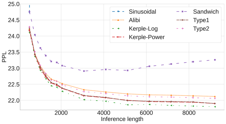
(a) Wikitext-103

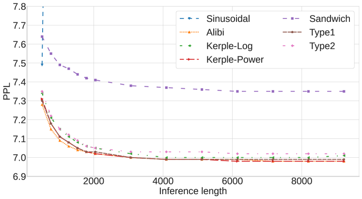
(b) Books

(c) Github

(d) WikiBook

Figure 3: Sufficiency validation on Wikitext-103, Books, Github, WikiBook datasets. To test length extrapolation capability, we lengthen inference sequences from 512 to 9216 tokens and plot the testing PPLs of our proposed Type 1 and Type 2 RPEs, as well as Alibi, Kerple, and Sandwich. All these methods are stable in PPL. For methods that cannot extrapolate, e.g.,  Sinusoidal, its PPL grows rapidly.

scaling the inference sequence length from 512 to 9216 tokens. As shown in Figure 4, the PPLs of both RPEs grow rapidly as the length of the testing sequence increases. It de-

(a) Wikitext-103

(b) Books

(c) Github

(d) WikiBook

Figure 4: Necessity validation on Wikitext-103, Books, Github, WikiBook datasets. We select two RPEs that do not satisfying Theorem 0.4, e.g., $b_{n}=\frac{1}{n}$ and $b_{n}=\frac{1}{n\ln n}$. We increase the inference sequence length from 512 to 9216 tokens and plot the testing PPLs for them. Their PPLs increase rapidly as the inference sequence lengthens, whereas Type 1 remains stable.

monstrates that both of them cannot extrapolate. We also include Type 1 RPE in Figure 4 as a reference that can extrapolate. Detailed numerical results can be found in Table 6

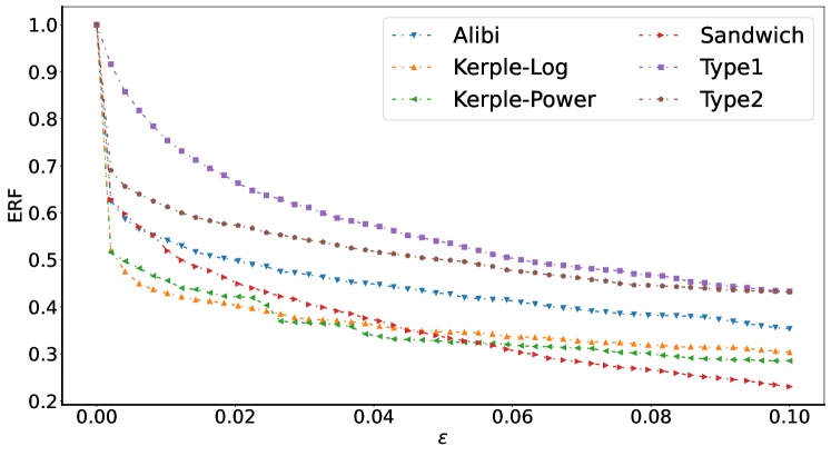
(a) Wikitext-103

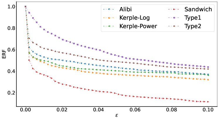
(b) Books

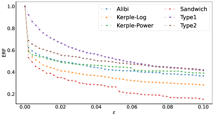
(c) Github

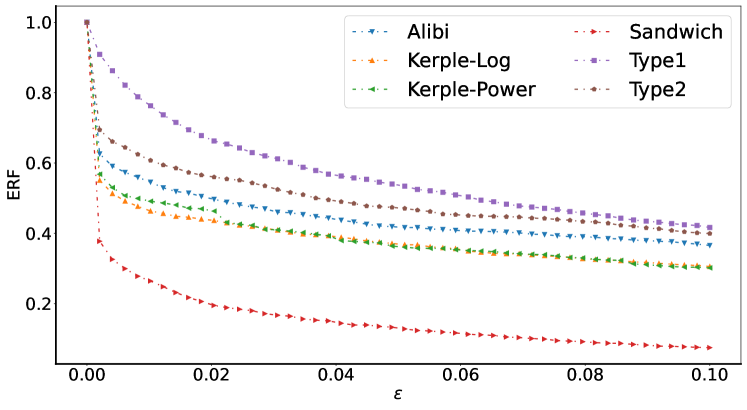
(d) wikibook

Figure 5: Visualization of ERF We plot the ERF for Alibi, Kerple, Sandwich and our proposed Type 1 and Type 2 methods on Wikitext-103, Books, Github, and WikiBook datasets using trained models. By comparing with Figure 6, we can find that the overall trend of ERF matches the trend of TRF. ERF is normalized for better visualization.

from Appendix.

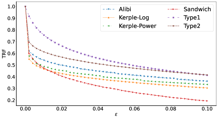
Figure 6: Visualization of TRF. We numerically plot TRFs for existing methods and our proposed method. TRF is normalized for visualization. The TRF of Type 1 is larger than Type 2, which matches the Theorem 0.5 and our analysis.

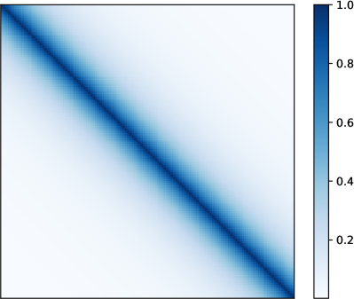
(a) Type1	(b) Type2

Figure 7: Visualization of RPE. We plot the heatmap of $\exp(\text{RPE})$ for Type 1 and Type 2. Type 2 concentrates weights on closer neighboring tokens than Type 1, indicating a smaller TRF. We also visualize other methods in Appendix.

Validating TRF

We validate our proposed TRF by comparing the trend between the TRF and ERF. We plot the TRFs and ERFs of the Alibi, Kerple, Sandwich, and our proposed RPEs on the aforementioned datasets. As observed in Figure 6 and Figure 5, while the curves vary across datasets, TRF estimates a similar overall trend of ERFs.

Visualizing RPE

We visualize the weighting schemes of Type 1 and Type 2 in Figure 7, i.e., the heatmap of $\exp(\text{RPE})$. Type 2 concentrates weights on closer neighboring tokens than Type 1, indicating a smaller TRF and ERF as shown in Figure 6 and Figure 5. We also visualize other methods in Appendix.

Conclusion

In this paper, we explore the secrets of transformer length extrapolation in language modeling. We first make a hypothesis about extrapolation and then derived the sufficient conditions for RPE to have the length extrapolation property. A thorough mathematical analysis reveals that a transformer model is certain to be capable of length extrapolation if the series that corresponds to the exponential of its RPE converges. This observation brings an extra bonus: we can estimate TRFs of RPEs solely based on their formulations. We chose two new RPEs that satisfy the conditions and two that do not to empirically prove the sufficiency of the conditions on four widely used datasets. We also validated our TRFs by comparing them with ERFs on these datasets as well. The results show that our TRFs can accurately reflect the actual receptive fields of RPEs before training.

Supplementary Material

Appendix A Mathematical notations

Notation	Meaning
$\mathbf{X}$	Hidden state.
$\mathbf{Q},\mathbf{K},\mathbf{V}$	Query, key, value.
$\mathbf{O}$	Attention output.
$d$	Feature dimension.
$\mathbf{m}^{\top}_{s}$	$s$-th row of matrix $M$.

Table 2: Mathematical notations used in the paper.

Appendix B Examples

In this section, we use Alibi (Press, Smith, and Lewis 2022), Kerple (Chi et al. 2022), and Sandwich (Chi, Fan, and Rudnicky 2022) as examples to support the discovered sufficient conditions 16 for length extrapolation.

Alibi The form of Alibi can be written as:

$$b_{t}=\exp(-kt),k>0.$$ (30)

According to the convergence of geometric series:

$$\lim_{i\to\infty}B_{ii}=\sum_{t=0}^{i-1}\exp(-kt)<\infty,$$ (31)

which satisfies our observed conditions.

Kerple Kerple proposes two forms of RPEs: log and power. We discuss them separately.

The formulation of the Log variant can be expressed as:

$$b_{t}=\exp(-r\log\left(1+kt\right))=\frac{1}{(1+kt)^{r}}$$ (32)

where r,k¿0r, k ¿ 0. In Kerple, r,kr, k are learnable. Based on Theorem 0.4, to enable the model to extrapolate, we must add the restriction that r¿1r ¿ 1 because:

$$\frac{1}{(1+kt)^{r}}\sim\frac{1}{k^{r}t^{r}},$$ (33)

In empirical analysis, we will show that when r=1r= 1, the model cannot extrapolate. We also checked the trained model from Kerple and found this condition is met.

The Ploy variant can be written as:

$$b_{t}=\exp(-kt^{r}),0<r\leq 2.$$ (34)

Since

$$b_{t}\leq\exp(-kt),t\to\infty.$$ (35)

according to the convergence of geometric series, we have:

$$\lim_{i\to\infty}B_{ii}=\lim_{i\to\infty}\sum_{t=0}^{i-1}\exp(-kt^{r})<\infty.$$ (36)

which satisfies our observed conditions.

Sandwich Given the formulation of Sandwich:

$$b_{t}=\exp\left(k\left(\sum_{j=1}^{d/2}\cos\left(\frac{t}{r^{2j/d}}\right)-\frac{d}{2}\right)\right),k>0,r>0.$$

We first do the following transformations:

$$b_{t} =\exp\left(k\left(\sum_{j=1}^{d/2}\left(\cos\left(\frac{t}{r^{2j/d}}\right)-1\right)\right)\right)$$ (37)

$$=\prod_{j=1}^{d/2}\exp\left(k\left(\cos\left(\frac{t}{r^{2j/d}}\right)-1\right)\right),$$

then make a partition over $j$:

$$\frac{t}{r^{2j/d}}\geq\frac{\pi}{2},$$ (38)

which is equivalent to:

$$2t \geq\pi r^{2j/d},\frac{2t}{\pi}\geq r^{2j/d},$$ (39)

$$\log_{r}\left(\frac{2t}{\pi}\right) \geq 2j/d,j\leq\frac{d\log_{r}\left(\frac{2t}{\pi}\right)}{2}\triangleq f(t).$$

Therefore we have:

$$b_{t} =\prod_{1\leq j\leq f(t)}\exp\left(k\left(\cos\left(\frac{t}{r^{2j/d}}\right)-1\right)\right)$$ (40)

$$\times\prod_{f(t)<j\leq d/2}\exp\left(k\left(\cos\left(\frac{t}{r^{2j/d}}\right)-1\right)\right).$$

For the first part:

$$\cos\left(\frac{t}{r^{2j/d}}\right)-1<-1.$$ (41)

For the second part:

$$\cos\left(\frac{t}{r^{2j/d}}\right)-1<0.$$ (42)

Then:

$$\beta_{t} \leq\prod_{1\leq j\leq f(t)}\exp(-k)$$ (43)

$$=\exp(-k\lfloor f(t)\rfloor)$$

$$\leq\exp(k)\exp(-kf(t))$$

$$=\exp(k)\exp\left(-\frac{kd\log_{r}\left(\frac{2t}{\pi}\right)}{2}\right)\triangleq g(t).$$

According to Rabbe’s test (Knopp 1956):

$$t\left(\frac{g(t)}{g({t+1})}-1\right) =t\left(\exp\left(\frac{kd}{2}\log_{r}\frac{2t+2}{2t}\right)-1\right)$$ (44)

$$=t\left(\exp\left(\frac{kd}{2}\log_{r}\left(1+\frac{1}{t}\right)\right)-1\right)$$

$$\sim t\left(\frac{kd}{2}\log_{r}\left(1+\frac{1}{t}\right)+O\left(\frac{1}{t^{2}}\right)\right)$$

$$\sim t\left(\frac{kd}{2\ln r}\left(\frac{1}{t}-\frac{1}{2t^{2}}\right)+O\left(\frac{1}{t^{2}}\right)\right)$$

$$\to\frac{kd}{2\ln r},$$

if:

$$\frac{kd}{2\ln r}<1,\quad d<\frac{2\ln r}{k},$$ (45)

then the series converges.

Appendix C TRF example

We use Alibi as an example to show the calculation of TRF. The $B_{ij}$ of Alibi can be written as:

$$B_{ij}=\sum_{i=0}^{j-1}\exp(-i)=\frac{1-\exp(-j)}{1-\exp(-1)},B=\frac{1}{1-\exp(-1)}$$ (46)

The TRF of Alibi can be calculated as:

$$n_{\mathrm{the}}(\epsilon) =\inf_{j}\left(B_{ij}>B(1-\epsilon)\right)$$ (47)

$$=\inf_{j}\left(1-\exp(-j)>1-\epsilon\right)=\Theta(-\log\epsilon).$$

where $\Theta$ represents the upper and lower asymptotic bound.

Appendix D Configurations

Data	WikiText-103	Others
Decoder layers	6	12
Hidden dimensions	512	768
Number of heads	8	12
FFN dimensions	2048	3072
Tokenizer method	BPE	BPE
Src Vocab size	50265	50265
Sequence length	512	512
Total batch size	128	128
Number of updates/epochs	50k updates	50k updates
Warmup steps/epochs	4k steps	4k steps
Peak learning rate	5e-4	5e-4
Learning rate scheduler	Inverse sqrt	Inverse sqrt
Optimizer	Adam	Adam
Adam $\epsilon$	1e-8	1e-8
Adam $(\beta_{1},\beta_{2})$	(0.9, 0.98)	(0.9, 0.98)
Weight decay	0.01	0.01

Table 3: Detailed training configurations used in our experiments. “Total batch size” means $\mathrm{batch\_per\_gpu}\times\mathrm{update\_freq}\times\mathrm{num\_gpus}$.

Appendix E Pseudocode for TRF and ERF visualization

⬇

1import torch

2

3def draw(array, n=50):

4 epsilon = torch.flip(torch.linspace(0, 1, n), dims=[0])

5 index = torch.zeros(n)

6 cusum = torch.sum(array)

7 m = len(array)

8 s = 0

9 i = 0

10 for j in range(m):

11 eps = epsilon[i]

12 while s >= cusum * (1 - eps) and i < n:

13 index[i] = j

14 if i < n - 1:

15 i += 1

16 else:

17 break

18 eps = epsilon[i]

19 s += array[j]

20 while i < n:

21 index[i] = m

22 i += 1

23

24 return index / m, epsilon

Appendix F Detailed Experimental Results

Wikitext-103
Length	Sinusoidal	Alibi	Kerple-Log	Kerple-Power	Sandwich	Type1	Type2
512	24.73	24.22	24.12	24.18	24.76	24.25	24.29
768	41.08	23.45	23.36	23.42	24.04	23.43	23.51
1024	62.71	23.06	22.93	22.98	23.63	23.03	23.09
1280	83.81	22.83	22.67	22.73	23.39	22.77	22.83
1536	102.28	22.66	22.45	22.54	23.21	22.55	22.63
1792	121.98	22.60	22.41	22.47	23.18	22.50	22.59
2048	138.17	22.52	22.28	22.37	23.08	22.38	22.48
3072	194.43	22.33	22.02	22.14	22.91	22.15	22.27
4096	259.55	22.26	21.97	22.08	22.96	22.09	22.21
5120	289.79	22.20	21.86	22.00	22.93	21.99	22.14
6144	337.46	22.17	21.87	21.96	23.06	21.97	22.11
7168	376.41	22.16	21.84	21.95	23.13	21.96	22.10
8192	406.95	22.14	21.82	21.94	23.20	21.95	22.08
9216	423.92	22.12	21.80	21.90	23.26	21.90	22.06
Books
Length	Sinusoidal	Alibi	Kerple-Log	Kerple-Power	Sandwich	Type1	Type2
512	7.49	7.28	7.34	7.31	7.64	7.30	7.35
768	10.43	7.15	7.21	7.18	7.55	7.18	7.22
1024	13.32	7.09	7.15	7.11	7.49	7.11	7.15
1280	15.53	7.06	7.11	7.08	7.47	7.08	7.12
1536	17.47	7.04	7.08	7.05	7.44	7.05	7.09
1792	19.02	7.03	7.06	7.03	7.42	7.03	7.06
2048	20.55	7.02	7.05	7.02	7.41	7.03	7.05
3072	24.70	7.00	7.02	7.00	7.38	7.00	7.03
4096	27.57	6.99	7.00	6.99	7.37	6.99	7.03
5120	29.54	6.99	7.00	6.99	7.36	6.99	7.03
6144	31.59	6.99	7.00	6.98	7.35	6.99	7.02
7168	32.41	6.98	7.00	6.98	7.35	6.99	7.02
8192	34.35	6.98	7.00	6.98	7.35	6.99	7.02
9216	34.70	6.98	7.01	6.98	7.35	6.99	7.02

Table 4: Sufficiency validation on Wikitext-103 and Books datasets. To test the length extrapolation capability, we lengthen the inference sequence from 512 to 9216 and compute PPLs of our proposed Type 1 and Type 2 RPEs, as well as Alibi, Kerple, and Sandwich. All these methods are stable in PPL. For methods that cannot extrapolate, e.g.,  Sinusoidal, its PPL grows rapidly.

Github
Length	Sinusoidal	Alibi	Kerple-Log	Kerple-Power	Sandwich	Type1	Type2
512	2.29	2.25	2.24	2.25	2.29	2.25	2.25
768	3.98	2.16	2.16	2.16	2.20	2.16	2.16
1024	7.91	2.12	2.12	2.12	2.16	2.12	2.12
1280	12.97	2.10	2.09	2.09	2.14	2.09	2.09
1536	18.66	2.09	2.07	2.08	2.12	2.08	2.08
1792	24.08	2.08	2.06	2.07	2.11	2.07	2.07
2048	30.02	2.07	2.05	2.07	2.10	2.06	2.06
3072	51.64	2.06	2.03	2.05	2.08	2.04	2.04
4096	70.62	2.05	2.02	2.04	2.07	2.03	2.03
5120	89.78	2.05	2.02	2.04	2.07	2.03	2.03
6144	101.28	2.05	2.01	2.04	2.06	2.03	2.03
7168	117.21	2.05	2.01	2.04	2.06	2.03	2.03
8192	130.15	2.05	2.01	2.03	2.06	2.02	2.03
9216	143.17	2.05	2.01	2.03	2.05	2.02	2.03
Wikibook
Length	Sinusoidal	Alibi	Kerple-Log	Kerple-Power	Sandwich	Type1	Type2
512	17.98	17.64	17.65	17.62	18.21	17.68	17.70
768	29.66	17.04	17.03	17.03	17.63	17.07	17.08
1024	47.31	16.76	16.73	16.73	17.35	16.76	16.80
1280	65.13	16.62	16.54	16.56	17.16	16.58	16.61
1536	83.16	16.51	16.41	16.44	17.04	16.44	16.49
1792	100.46	16.49	16.33	16.41	16.95	16.39	16.44
2048	116.94	16.43	16.26	16.36	16.89	16.31	16.39
3072	172.09	16.39	16.13	16.31	16.75	16.23	16.33
4096	231.86	16.39	16.14	16.29	16.73	16.24	16.36
5120	277.59	16.35	16.10	16.26	16.68	16.21	16.32
6144	312.17	16.35	16.12	16.25	16.66	16.22	16.32
7168	349.08	16.34	16.19	16.24	16.71	16.26	16.33
8192	390.81	16.35	16.22	16.25	16.71	16.30	16.36
9216	412.06	16.33	16.23	16.24	16.70	16.28	16.33

Table 5: Sufficiency validation on Github, WikiBook datasets. To test the length extrapolation capability, we lengthen the inference sequence from 512 to 9216 and compute PPLs of our proposed Type 1 and Type 2 RPEs, as well as Alibi, Kerple, and Sandwich. All these methods are stable in PPL. For methods that cannot extrapolate, e.g.,  Sinusoidal, its PPL grows rapidly.

	Wikitext-103		Books		Github		Wikibook
Length	$\frac{1}{n}$	$\frac{1}{n\ln n}$	$\frac{1}{n}$	$\frac{1}{n\ln n}$	$\frac{1}{n}$	$\frac{1}{n\ln n}$	$\frac{1}{n}$	$\frac{1}{n\ln n}$
512	24.67	24.64	7.40	7.35	2.28	2.27	17.91	17.90
768	23.87	23.81	7.28	7.24	2.19	2.18	17.28	17.28
1024	23.53	23.44	7.27	7.19	2.17	2.15	17.21	17.12
1280	23.50	23.25	7.41	7.20	2.19	2.15	17.70	17.28
1536	23.66	23.13	7.65	7.24	2.31	2.19	18.86	17.72
1792	24.20	23.22	7.97	7.30	2.52	2.28	20.74	18.65
2048	24.80	23.26	8.34	7.39	2.85	2.39	23.31	19.82
3072	28.31	23.65	9.97	7.82	5.05	3.15	38.46	27.94
4096	33.18	24.41	11.84	8.29	9.13	4.35	59.51	40.06
5120	37.65	25.01	14.15	8.80	15.79	5.93	84.60	55.12
6144	43.20	25.80	16.64	9.27	25.00	8.03	112.30	71.08
7168	48.07	26.39	18.99	9.73	36.01	10.26	140.34	89.79
8192	52.85	27.00	22.06	10.06	49.20	12.80	173.55	108.85
9216	58.46	27.63	26.34	10.65	76.78	16.35	204.10	133.36

Table 6: Necessity validation on Wikitext-103, Books, Github, WikiBook datasets. We select two RPEs that do not satisfying Theorem 0.4, e.g., $b_{n}=\frac{1}{n}$ and $b_{n}=\frac{1}{n\ln n}$. We increase the inference sequence length from 512 to 9216 and compute the testing PPLs of them. Their PPLs increase rapidly as the inference sequence lengthens.

Appendix G Heatmap

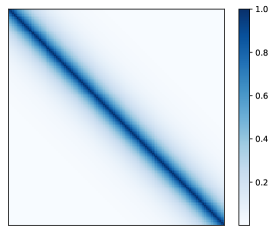
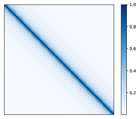
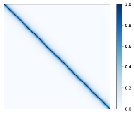
(a) Alibi	(b) Kerple-Log	(c) Kerple-Power
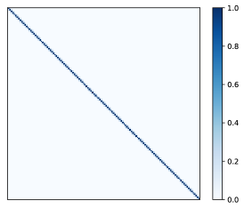
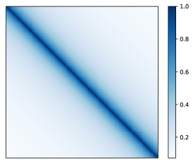
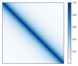
(d) Sandwich	(e) $\frac{1}{n}$	(f) $\frac{1}{n\ln n}$

Figure 8: Visualization of RPE. We additionally plot the heatmap of $\exp(\text{RPE})$ for all methods. Note that all methods are concentrated near the diagonal, including $\frac{1}{n},\frac{1}{n\ln n}$, which shows that the concentration is not enough to guarantee extrapolation.

References

- Akbari et al. (2021) Akbari, H.; Yuan, L.; Qian, R.; Chuang, W.-H.; Chang, S.-F.; Cui, Y.; and Gong, B. 2021. Vatt: Transformers for multimodal self-supervised learning from raw video, audio and text. In arXiv preprint arXiv:2104.11178.
- Beltagy, Peters, and Cohan (2020) Beltagy, I.; Peters, M. E.; and Cohan, A. 2020. Longformer: The Long-Document Transformer. In arXiv:2004.05150.
- Chi et al. (2022) Chi, T.-C.; Fan, T.-H.; Ramadge, P. J.; and Rudnicky, A. I. 2022. KERPLE: Kernelized Relative Positional Embedding for Length Extrapolation. ArXiv, abs/2205.09921.
- Chi, Fan, and Rudnicky (2022) Chi, T.-C.; Fan, T.-H.; and Rudnicky, A. I. 2022. Receptive Field Alignment Enables Transformer Length Extrapolation. ArXiv, abs/2212.10356.
- Cho et al. (2014) Cho, K.; van Merriënboer, B.; Gulcehre, C.; Bahdanau, D.; Bougares, F.; Schwenk, H.; and Bengio, Y. 2014. Learning Phrase Representations using RNN Encoder–Decoder for Statistical Machine Translation. In Proceedings of the 2014 Conference on Empirical Methods in Natural Language Processing (EMNLP), 1724–1734. Doha, Qatar: Association for Computational Linguistics.
- Devlin et al. (2019) Devlin, J.; Chang, M.-W.; Lee, K.; and Toutanova, K. 2019. BERT: Pre-training of Deep Bidirectional Transformers for Language Understanding. In Proceedings of the 2019 Conference of the North American Chapter of the Association for Computational Linguistics: Human Language Technologies, Volume 1 (Long and Short Papers), 4171–4186. Minneapolis, Minnesota: Association for Computational Linguistics.
- Dosovitskiy et al. (2020) Dosovitskiy, A.; Beyer, L.; Kolesnikov, A.; Weissenborn, D.; Zhai, X.; Unterthiner, T.; Dehghani, M.; Minderer, M.; Heigold, G.; Gelly, S.; et al. 2020. An image is worth 16x16 words: Transformers for image recognition at scale. arXiv preprint arXiv:2010.11929.
- Gao et al. (2020) Gao, L.; Biderman, S.; Black, S.; Golding, L.; Hoppe, T.; Foster, C.; Phang, J.; He, H.; Thite, A.; Nabeshima, N.; Presser, S.; and Leahy, C. 2020. The Pile: An 800GB Dataset of Diverse Text for Language Modeling. In arXiv preprint arXiv:2101.00027.
- Gehring et al. (2017) Gehring, J.; Auli, M.; Grangier, D.; Yarats, D.; and Dauphin, Y. N. 2017. Convolutional sequence to sequence learning. In International Conference on Machine Learning, 1243–1252. PMLR.
- Gong, Chung, and Glass (2021) Gong, Y.; Chung, Y.-A.; and Glass, J. 2021. AST: Audio Spectrogram Transformer. In Proc. Interspeech 2021, 571–575.
- Gulati et al. (2020) Gulati, A.; Chiu, C.-C.; Qin, J.; Yu, J.; Parmar, N.; Pang, R.; Wang, S.; Han, W.; Wu, Y.; Zhang, Y.; and Zhang, Z., eds. 2020. Conformer: Convolution-augmented Transformer for Speech Recognition.
- Hao et al. (2024) Hao, D.; Mao, Y.; He, B.; Han, X.; Dai, Y.; and Zhong, Y. 2024. Improving Audio-Visual Segmentation with Bidirectional Generation. In Proceedings of the AAAI Conference on Artificial Intelligence.
- Hershey et al. (2016) Hershey, S.; Chaudhuri, S.; Ellis, D. P. W.; Gemmeke, J. F.; Jansen, A.; Moore, R. C.; Plakal, M.; Platt, D.; Saurous, R. A.; Seybold, B.; Slaney, M.; Weiss, R. J.; and Wilson, K. W. 2016. CNN architectures for large-scale audio classification. 2017 IEEE International Conference on Acoustics, Speech and Signal Processing (ICASSP), 131–135.
- Hochreiter and Schmidhuber (1997) Hochreiter, S.; and Schmidhuber, J. 1997. Long short-term memory. Neural computation, 9(8): 1735–1780.
- Kim (2014) Kim, Y. 2014. Convolutional Neural Networks for Sentence Classification. In Conference on Empirical Methods in Natural Language Processing.
- Knopp (1956) Knopp, K. 1956. Infinite sequences and series. Courier Corporation.
- Liu et al. (2019) Liu, Y.; Ott, M.; Goyal, N.; Du, J.; Joshi, M.; Chen, D.; Levy, O.; Lewis, M.; Zettlemoyer, L.; and Stoyanov, V. 2019. Roberta: A robustly optimized bert pretraining approach. arXiv preprint arXiv:1907.11692.
- Liu et al. (2022) Liu, Z.; Li, D.; Lu, K.; Qin, Z.; Sun, W.; Xu, J.; and Zhong, Y. 2022. Neural architecture search on efficient transformers and beyond. arXiv preprint arXiv:2207.13955.
- Liutkus et al. (2021) Liutkus, A.; Cífka, O.; Wu, S.-L.; Simsekli, U.; Yang, Y.-H.; and Richard, G. 2021. Relative positional encoding for transformers with linear complexity. In International Conference on Machine Learning, 7067–7079. PMLR.
- Lu et al. (2022) Lu, K.; Liu, Z.; Wang, J.; Sun, W.; Qin, Z.; Li, D.; Shen, X.; Deng, H.; Han, X.; Dai, Y.; and Zhong, Y. 2022. Linear video transformer with feature fixation. arXiv preprint arXiv:2210.08164.
- Merity et al. (2016) Merity, S.; Xiong, C.; Bradbury, J.; and Socher, R. 2016. Pointer Sentinel Mixture Models. In arXiv:1609.07843.
- Ott et al. (2019) Ott, M.; Edunov, S.; Baevski, A.; Fan, A.; Gross, S.; Ng, N.; Grangier, D.; and Auli, M. 2019. fairseq: A fast, extensible toolkit for sequence modeling. arXiv preprint arXiv:1904.01038.
- Press, Smith, and Lewis (2022) Press, O.; Smith, N.; and Lewis, M. 2022. Train Short, Test Long: Attention with Linear Biases Enables Input Length Extrapolation. In International Conference on Learning Representations.
- Qin et al. (2023a) Qin, Z.; Han, X.; Sun, W.; He, B.; Li, D.; Li, D.; Dai, Y.; Kong, L.; and Zhong, Y. 2023a. Toeplitz Neural Network for Sequence Modeling. In The Eleventh International Conference on Learning Representations.
- Qin et al. (2022a) Qin, Z.; Han, X.; Sun, W.; Li, D.; Kong, L.; Barnes, N.; and Zhong, Y. 2022a. The Devil in Linear Transformer. In Proceedings of the 2022 Conference on Empirical Methods in Natural Language Processing, 7025–7041. Abu Dhabi, United Arab Emirates: Association for Computational Linguistics.
- Qin et al. (2023b) Qin, Z.; Li, D.; Sun, W.; Sun, W.; Shen, X.; Han, X.; Wei, Y.; Lv, B.; Yuan, F.; Luo, X.; Qiao, Y.; and Zhong, Y. 2023b. Scaling TransNormer to 175 Billion Parameters. In arXiv preprint 2307.14995.
- Qin et al. (2022b) Qin, Z.; Sun, W.; Deng, H.; Li, D.; Wei, Y.; Lv, B.; Yan, J.; Kong, L.; and Zhong, Y. 2022b. cosFormer: Rethinking Softmax In Attention. In International Conference on Learning Representations.
- Qin et al. (2023c) Qin, Z.; Sun, W.; Lu, K.; Deng, H.; Li, D.; Han, X.; Dai, Y.; Kong, L.; and Zhong, Y. 2023c. Linearized Relative Positional Encoding. arXiv preprint arXiv:2307.09270.
- Qin, Yang, and Zhong (2023) Qin, Z.; Yang, S.; and Zhong, Y. 2023. Hierarchically gated recurrent neural network for sequence modeling. NeurIPS.
- Qin and Zhong (2023) Qin, Z.; and Zhong, Y. 2023. Accelerating Toeplitz Neural Network with Constant-time Inference Complexity. In Proceedings of the 2023 Conference on Empirical Methods in Natural Language Processing. Association for Computational Linguistics.
- Su et al. (2021) Su, J.; Lu, Y.; Pan, S.; Wen, B.; and Liu, Y. 2021. Roformer: Enhanced transformer with rotary position embedding. arXiv preprint arXiv:2104.09864.
- Sun et al. (2022a) Sun, J.; Zhong, G.; Zhou, D.; Li, B.; and Zhong, Y. 2022a. Locality Matters: A Locality-Biased Linear Attention for Automatic Speech Recognition. arXiv preprint arXiv:2203.15609.
- Sun et al. (2022b) Sun, W.; Qin, Z.; Deng, H.; Wang, J.; Zhang, Y.; Zhang, K.; Barnes, N.; Birchfield, S.; Kong, L.; and Zhong, Y. 2022b. Vicinity Vision Transformer. IEEE Transactions on Pattern Analysis and Machine Intelligence, (01): 1–14.
- Vaswani et al. (2017) Vaswani, A.; Shazeer, N.; Parmar, N.; Uszkoreit, J.; Jones, L.; Gomez, A. N.; Kaiser, Ł.; and Polosukhin, I. 2017. Attention is all you need. Advances in neural information processing systems, 30.
- Wettig et al. (2022) Wettig, A.; Gao, T.; Zhong, Z.; and Chen, D. 2022. Should You Mask 15% in Masked Language Modeling? In arXiv:2202.08005.
- Zhu et al. (2015) Zhu, Y.; Kiros, R.; Zemel, R.; Salakhutdinov, R.; Urtasun, R.; Torralba, A.; and Fidler, S. 2015. Aligning Books and Movies: Towards Story-Like Visual Explanations by Watching Movies and Reading Books. In The IEEE International Conference on Computer Vision (ICCV).