GWDALI: A Fisher-matrix based software for gravitational wave parameter-estimation beyond Gaussian approximation

Abstract

We introduce GWDALI, a new Fisher-matrix, python based software that computes likelihood gradients to forecast parameter-estimation precision of arbitrary network of terrestrial gravitational wave detectors observing compact binary coalescences. The main new feature with respect to analogous software is to assess parameter uncertainties beyond Fisher-matrix approximation, using the derivative approximation for Likelihood (DALI). The software makes optional use of the LSC algorithm library LAL and the stochastic sampling algorithm Bilby, which can be used to perform Monte-Carlo sampling of exact or approximate likelihood functions. As an example we show comparison of estimated precision measurement of selected astrophysical parameters for both the actual likelihood, and for a variety of its derivative approximations, which turn out particularly useful when the Fisher matrix is not invertible.

[first]organization=Departamento de Física Teórica e Experimental, city=Natal, state=RN, country=Brazil

[ufrn]organization=Instituto de Física Teórica, UNESP/ICTP-SAIFR, city=São Paulo, state=SP, country=Brazil

1 Introduction

The advent of Gravitational Wave (GW) astronomy [1], with the detections made by the LIGO [2] and Virgo [3] detectors, naturally calls for investigating which physical quantity and how well it can be measured with the observations made possible in this new gravitational channel.

The detector network should be enriched by the Japanese KAGRA [4] already in the ongoing fourth science run of the so-called second generation GW detectors, and by the Indian Indigo [5] by the end of the current decade. For the next decade, additional third generation detectors are foreseen, namely the European Einstein Telescope (ET) [6] and the North-American Cosmic Explorer (CE) [7].

While detections in the future may not be limited to compact binary coalescences, they represent the totality of detections so far, and they are expected to be the key observables for future observatories as well. It is then natural to ask ourselves for expectations and forecast of precision measures of astrophysical source parameters, how they depends on the intrinsic detector feature, like spectral noise density, and localization and orientation of the detectors composing the network.

Parameter estimation is naturally performed within a Bayesian inference framework, which allows determination of most likely values of signal model parameter as well as their confidence interval. A common tool for rapid precision forecast is the Fisher matrix approximation, which consists in approximating the logarithm of the likelihood in the proximity of its maximum value with a Taylor expansion truncated at quadratic order. By inverting the matrix of second derivatives of the log-likelihood with respect to all parameters one can then obtain the covariance matrix, which gives direct assessment of marginalized uncertainties of physical parameters [8]. On one hand the Fisher matrix approximation is ubiquitous in data analyses, as an invaluable tool to provide analytic and easy-to-compute estimates of parameter uncertainties, on the other hand there are cases in which it can fail, e.g. in presence of approximately flat directions and/or correlations among parameters, giving rise to zero determinant second derivative matrix.

In this case it is natural to investigate how higher order approximations may perform with respect to the quadratic one and/or the complete likelihood. The goal of the present work is to introduce a tool to perform a suitable Taylor expansion of the derivative approximation of the log-likelihood. This is implemented in the publicly available python code GWDALI, complementing standard Fisher matrix codes already available in literature like GWBENCH [9], GWFISH [10], and GWFAST [11].

In particular we borrow here the idea to use higher (than second) derivative approximations to the log-likelihood from [12], where the Derivative Approximation for LIkelihood (DALI) was first proposed in a general context and applied to cosmological examples, and from [13], where a first example of DALI applied to GW source parameter inference has been proposed.

The paper is structured as follows: in Sec. 2 we give an overview of parameter estimation for GW signal from coalescing binaries highlighting some known limit of the Fisher-matrix approximation, followed in Sec. 3 by a description of the DALI method. In Sec. 4 we give an example of the benefits of using GWDALI for estimating parameter uncertanties and finally in Sec. 5 we outline possible future applications and development of the GWDALI software.

2 Astrophysical parameter estimation for coalescing binaries and Fisher matrix

The coalescence of compact binary systems can be divided in three phases: inspiral, merger and ring-down. In particular the inspiral phase admits an analytic description in terms of approximations to General Relativity, the most successful of which in building waveform models has been the post-Newtonian approximation [14, 15]. The subsequent merger phase is in principle determined by the inspiral one, of which it is the continuation, and it has been described solved with numerical methods [16]. Finally the ring-down phase also admits an analytic description, in terms of damped exponentials, and several phenomenological models exist nowadays providing complete analytic waveforms encompassing the three phases, see e.g. [17, 18]. An exhaustive set of waveform approximant is available in the LSC algorithm library (LAL) [19], which are callable by python or C codes.

The binary systems of interest for current detectors are expected to be in circular orbits, as angular momentum is more efficiently radiated than energy. Orbits are indeed expected to circularize in the early stage of inspiral [20], leaving little or no eccentricity when reaching the LIGO/Virgo band ($10-10^{4}$ Hz), which is not too distant from the merger frequency $f_{m}$, which can be roughly approximated by $(2\pi M)^{-1}$, being $M$ the total mass of the binary system, obtaining $f_{m}\sim 32$kHz$(M/M_{\odot})^{-1}$. The astrophysical parameters defining a circular binary coalescences are 15 [21], organized in two categories [22] according to if they affect the morphology of the waveform (intrinsic), or just its overall shape (extrinsic). The 15 parameters are summarized in Tab. 1.

Intrinsic parameters	Extrinsic parameters
$M_{c}$, $\eta$, $\vec{S}_{1}$, $\vec{S}_{2}$	$d_{L}$, $\psi$, $\iota$, $\phi$, $\alpha$, $\beta$, $t$

Table 1: Parameters defining the observation of a binary system observation (whose constituents are treated as point-like object), divided between intrinsic ($m_{1,2}$ are the constituent masses, $\vec{S}_{1,2}$ are the binary constituent spin vectors) and extrinsic (see text).

Given the time series of the output of the $i$-th detector $d_{i}$ and a template signal $h_{t_{i}}$, the log-likelihood for astrophysical parameter inference is proportional the norm-squared $||d_{i}-h_{t_{i}}||^{2}$, where the norm is inherited from the scalar product

$$\langle h_{1},h_{2}\rangle=2\int_{0}^{\infty}\frac{\tilde{h}_{1}(f)\tilde{h}_{2}^{*}(f)+\tilde{h}_{1}^{*}(f)\tilde{h}_{2}(f)}{S_{n}(f)}df\,,$$ (1)

where $S_{n}(f)$ is the one sided spectral noise density of the detector defined by averaging the noisy detector output:

$$\langle\tilde{n}(f)\tilde{n}^{*}(f^{\prime})\rangle\equiv\frac{1}{2}S_{n}(f)\delta(f-f^{\prime})\,.$$ (2)

The Einstein Telescope (ET) [6] and Cosmic Explorer (CE) [23] sensitivity curves adopted in this work are shown in Fig. 1.

The detector response to a GW is a linear combination of the two polarizations with weights given by the pattern functions $F_{+,\times}$, which depend on sky localization of the source (defined by polar angles $\alpha,\beta$) and the polarization angle $\psi$:

$$h_{d_{i}}=F_{+}(\alpha,\beta,\psi)h_{+}+F_{\times}(\alpha,\beta,\psi)h_{\times}\,.$$ (3)

The specific form of the pattern functions depend on the type of detector considered. For interferometric detectors with opening angle $\Omega$ they are, see ch. 7 of [24],

$$\begin{array}[]{rcl}F_{+}&=&f_{+}\cos(2\psi)+f_{\times}\sin(2\psi)\,,\\ F_{\times}&=&f_{\times}\cos(2\psi)-f_{+}\sin(2\psi)\,,\end{array}$$ (6)

with

$$\begin{array}[]{rcl}f_{+}&\equiv&\sin\Omega\frac{1}{2}(1+\cos^{2}\beta)\cos(2\alpha)\,,\\ f_{\times}&\equiv&-\sin\Omega\cos\beta\sin(2\alpha)\,.\end{array}$$ (9)

In the lowest order approximation (quadrupole formula) the polarizations for the inspiral phase admit a simple analytic form, see e.g. ch.4 of  [24]

$$\begin{array}[]{rcl}\displaystyle\tilde{h}_{+}(f)&=&\displaystyle\frac{1+\cos^{2}\iota}{2}\pi^{-2/3}\left(\frac{5}{24}\right)^{1/2}\frac{\mathcal{M}_{c}^{5/6}f^{-7/6}}{d_{L}}e^{i\Phi(f)}\,,\\ \displaystyle\tilde{h}_{\times}(f)&=&\displaystyle\cos\iota\,\pi^{-2/3}\left(\frac{5}{24}\right)^{1/2}\frac{\mathcal{M}_{c}^{5/6}f^{-7/6}}{d_{L}}ie^{i\Phi(f)}\,,\end{array}$$ (12)

where $\mathcal{M}_{c}$ is the redshifted chirp mass defined by $\mathcal{M}_{c}\equiv\eta^{3/5}M(1+z)$, with $M$ the intrinsic total mass $M\equiv m_{1}+m_{2}$, $\eta$ the symmetric mass ratio $\eta\equiv m_{1}m_{2}/M^{2}$, $z$ is the redshift and $\Phi(f)$ has an expansion known up to 4th perturbative order in terms of the PN expansion parameter $v^{2}\equiv(\pi Mf)^{2/3}$, see e.g. [25] and depends on $\eta$ and linearly on the arrival time $t$ and the phase $\phi$. Note that $\iota,\phi,\psi$ compose the three Euler angles defining the orientation of the source axis triad with respect to the observation one [26].

The log-likelihood vanishes when the template matches exactly the data, the Fisher matrix for the $i$-th detector being

$${\cal F}_{i,ab}=4{\cal R}e\int_{0}^{\infty}\frac{\partial_{\theta_{a}}\tilde{h}_{t_{i}}\partial_{\theta_{b}}\tilde{h}_{t_{i}}^{*}}{S_{n}(f)}df\,,$$ (13)

where dependence of $h_{t_{i}}$ (and $\tilde{h}_{t_{i}}$) upon parameters $\theta$ is understood in the notation. The $k$-th element of the diagonal of the inverse of the Fisher matrix, the covariance matrix, returns marginalized uncertainties for the $k$-th variable, which then crucially depend on correlation among parameters.

One of the obvious shortcomings of the Fisher matrix approximation is encountered when the Fisher matrix itself is not invertible, hence it is not possible to find the covariance matrix. This is exemplified in Fig. 2, where the result for $d_{L}$ of the four dimensional covariance matrix in $\{d_{L},\iota,\psi,\phi\}$ are displayed, as obtained with the code GWFISH for the ET detector (made of three interferometers arranged in a equilater triangles) and for CE (one $L$-shaped interferometer).

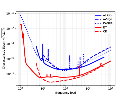
Figure 1: ET [27] and CE [28] noise spectral densities.

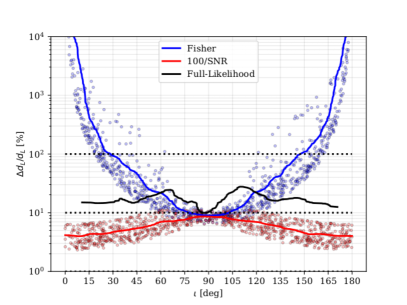
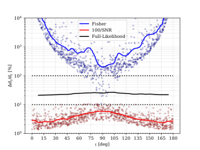
Figure 2: Example of $\Delta d_{L}/d_{L}$ vs. $\iota$ for a 4-dimensional Fisher matrix in the parameters: $\{d_{L},\iota,\psi,\phi\}$ from GWFISH code (blue line) [10], full likelihood for the same parameters (black) and for the analytic curve given by $100/SNR$ (red). GW signals are generated by equal mass spin-less binaries with $M=3M_{\odot}$ with TaylorF2 approximant [29], averaged over sky position and inclination angles for ET (left) and CE (right).

The increase of $d_{L}$ uncertainty, which is unbound for $\iota\to 0,\pi$ in the Fisher matrix approximation, is due to $det({\cal F})\to 0$ as $\iota\to 0,\pi$, signaling a degenerate direction in the parameter space, and invalidating the Gaussian approximation the Fisher matrix approach is based on. The fact that this is a spurious behaviour due to the Fisher approximation of the exact likelihood, is highlighted by the analaog quantity obtained by MonteCarlo sampling of the likelihood, black line in Fig. 2. We discuss in Sec. 3 a proposal about how to handle this problem.

2.1 Analytic Fisher Matrix Inversion

The inverse of the Fisher matrix is the covariance matrix, whose diagonal entries give the fully marginalized 1$\sigma$ errors (in the Gaussian approximation) of the corresponding parameters, which is probably the most useful property of the Fisher method. The diagonal entries of the covariance matrix are different depending on how many parameter one keeps fixed to the maximum likelihood values, i.e. they depend on the dimensionality of the Fisher matrix. As an example, the $d_{L}$ 1$\sigma$-uncertainty with all other parameters fixed can be computed as:

$$\left(\frac{\Delta d_{L}}{d_{L}}\right)^{2}=\frac{1}{SNR^{2}}=\frac{4||k||^{-2}}{\left[(1+\cos^{2}\iota)^{2}F_{+}^{2}+4cos^{2}\iota F_{\times}^{2}\right]}\,,$$ (14)

where using the inspiral expressions (12) one has

$$||k||^{2}\equiv\frac{5}{6}\frac{(G\mathcal{M}_{c})^{5/3}}{\pi^{4/3}d_{L}^{2}}\int_{0}^{\infty}\frac{f^{-7/3}}{S_{n}(f)}df\,,$$ (15)

and the $SNR$ is defined as the norm of the GW signal $h$ given the scalar product in eq. (1).

Marginalizing over $\iota$, instead of pinning it to its maximum likelihood value, shows the effect of correlations into determining parameter uncertainty. In this case, one can then read the $d_{L}$ uncertainty as

$$\left(\frac{\Delta d_{L}}{d_{L}}\right)^{2}=\frac{Cov(d_{L},d_{L})}{d_{L}^{2}}=\frac{\langle\partial_{\iota}h,\partial_{\iota}h\rangle}{d_{L}^{2}det({\cal F})}=||k||^{-2}\frac{4(\cos^{2}\iota F_{+}^{2}+F_{\times}^{2})}{\sin^{4}\iota(F_{+}F_{\times})^{2}}\,.$$ (16)

This is a simple example of how correlations among parameters can degrade the precision of individual parameters. In particular Figs. 3 report the analytic Fisher matrix prediction of the uncertainty estimate of $d_{L}$ as a function of the injected value of $\iota$ in two cases: 1-dimensional Fisher matrix and bi-dimensional for parameters $d_{L},\iota$ (sources are located above a CE-like detector).

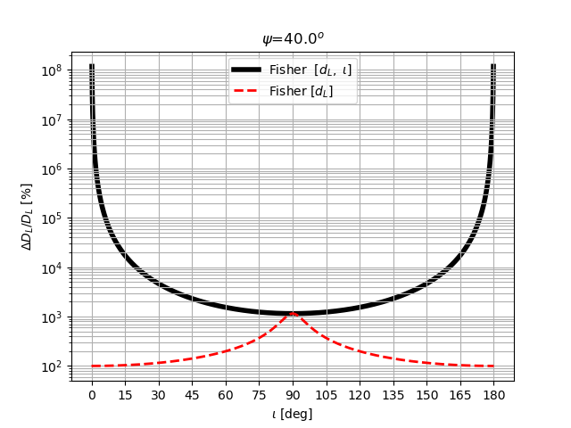
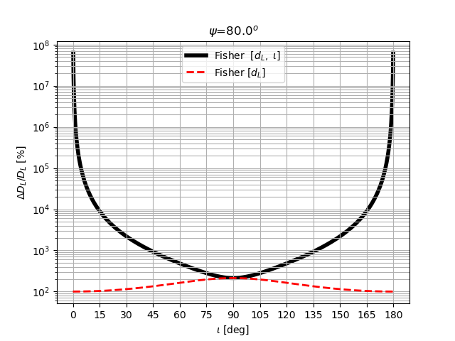
Figure 3: 1$\sigma$ relative uncertainty in $d_{L}$ fixing all other parameters (dashed red) or marginalizing over $\iota$ (solid black).

The presence of a zero eigenvalue in the Fisher matrix for $\iota\to 0,\pi$ denotes the existence of a flat direction, invalidating the Gaussian approximation. In this example such breakdown manifests itself by the divergence of the Fisher matrix prediction of $\Delta d_{L}$.

Note that standard recipes for obtaining the (pseudo-)inverse of a zero-determinant Fisher matrix are adopted in e.g. GWFISH [10] and GWFAST [11], where the Penrose method for generalized inverse [30] is implemented. Such method consists of excluding from the inversion the subspace corresponding to the kernel of the Fisher matrix. However identifying a zero eigenvalue numerically depends on an arbitrary threshold. We propose in the next section the application of higher derivative likelihood approximation to GW parameter estimation.

3 DALI algorithm for Gravitational Waves

Following the introduction of higher derivative in the likelihood expansion in [12], we now introduce the GWDALI implementation of likelihood beyond Gaussian order. Let $\theta$ be the set of GW parameters listed in Tab. 1. The Fisher matrix approximation relies on a Taylor expansion of the log-likelihood around the maximum likelihood value. Given the definition (1), the log-likelihood as the norm-squared of the difference between data and template, one has the straightforward Taylor expansion beyond quadratic order

$$\begin{array}[]{rcl}\log\mathcal{L}&=&\displaystyle-\frac{1}{2}||d_{i}-h_{t_{i}}(\theta)||^{2}\\ &\simeq&\displaystyle\log\mathcal{L}_{0}+\cancel{\sum_{a}\left(\partial_{a}\log\mathcal{L}\right)_{0}\Delta\theta_{a}}+\frac{1}{2!}\sum_{a,b}\left(\partial_{a}\partial_{b}\log\mathcal{L}\right)_{0}\Delta\theta^{ab}\\ &&\displaystyle+\frac{1}{3!}\sum_{a,b,c}\left(\partial_{a}\partial_{b}\partial_{c}\log\mathcal{L}\right)_{0}\Delta\theta^{abc}\\ &&\displaystyle+\frac{1}{4!}\sum_{a,b,c,d}\left(\partial_{a}\partial_{b}\partial_{c}\partial_{d}\log\mathcal{L}\right)_{0}\Delta\theta^{abcd}\\ &&\displaystyle+\frac{1}{5!}\sum_{a,b,c,d,e}\left(\partial_{a}\partial_{b}\partial_{c}\partial_{d}\partial_{e}\log\mathcal{L}\right)_{0}\Delta\theta^{abcde}+\ldots\,,\end{array}$$ (22)

where $\Delta\theta^{a}\equiv\theta^{a}-\theta^{a}_{0}$, $\Delta\theta^{a_{1}\dots a_{n}}\equiv\Delta\theta^{a_{1}}\dots\Delta\theta^{a_{n}}$ and the subscript “$0$” stand for maximum likelihood value of the parameters. The first order term of the Taylor expansion has been slashed out as it vanishes.

One can then define derivative tensors beyond the Fisher matrix

$$\begin{array}[]{ll}\text{Fisher Matrix: }{\cal F}_{ab}&\displaystyle\equiv-\left(\partial_{a}\partial_{b}\log\mathcal{L}\right)_{0}=4\sum_{i=1}^{N_{det}}{\cal R}e\int_{0}^{\infty}\left(\frac{\partial\tilde{h}_{t_{i}}}{\partial\theta^{a}}\frac{\partial\tilde{h}_{t_{i}}}{\partial\theta^{b}}\right)\frac{df}{S_{n}(f)}\\ &\displaystyle\equiv\left\langle\partial_{a}h|\partial_{b}h\right\rangle\,,\\ \text{Flexion Tensor: }{\cal S}_{abc}&\displaystyle\equiv-\left(\partial_{a}\partial_{b}\partial_{c}\log\mathcal{L}\right)_{0}\,,\\ \text{Quarxion Tensor: }{\cal Q}_{abcd}&\displaystyle\equiv-\left(\partial_{a}\partial_{b}\partial_{c}\partial_{d}\log\mathcal{L}\right)_{0}\,,\\ \text{P-Tensor: }\mathcal{P}_{abcde}&\displaystyle\equiv-\left(\partial_{a}\partial_{b}\partial_{c}\partial_{d}\partial_{e}\log\mathcal{L}\right)_{0}\,,\\ \text{H-Tensor: }\mathcal{H}_{abcdef}&\displaystyle\equiv-\left(\partial_{a}\partial_{b}\partial_{c}\partial_{d}\partial_{e}\partial_{f}\log\mathcal{L}\right)_{0}\,.\end{array}$$ (29)

The explicit expression of the symmetric derivative tensors at third order Taylor expansion ($O(\Delta\theta^{3})$), or Flexion term, is given by the addition of 3 terms that can be arranged as follows:

$${\cal S}_{abc}=\left\langle\partial_{a}h|\partial_{b}\partial_{c}h\right\rangle_{0}+(a\leftrightarrow b)+(a\leftrightarrow c)\,,$$ (30)

and its contribution to the likelihood is given by

$$\begin{array}[]{cl}\log\mathcal{L}_{3}&\displaystyle\equiv-\frac{1}{6}\sum_{a,b,c}{\cal S}_{abc}\Delta\theta^{abc}\\ &\displaystyle=-\frac{1}{2}\sum_{a,b,c}\left\langle\partial_{a}h|\partial_{b}\partial_{c}h\right\rangle_{0}\Delta\theta^{abc}\,,\end{array}$$ (33)

where at most second derivative of the waveform are involved. Note that an approximate log-likelihood truncated at $O(\Delta\theta^{3})$ is not negative semi-definite, causing a fundamental problem in the probabilistic interpretation of the likelihood.

However, as explained in [12], this problem is fixed by truncating the expansion in number of derivatives, rather than in powers of $\Delta\theta$. Going beyond Gaussian level then requires to collect all terms involving a given number of derivatives. To have a consistent expansion with two derivatives one needs to include the relevant part of the Quarxion term:

$$\begin{array}[]{cl}{\cal Q}_{abcd}=&\displaystyle\left[\left\langle\partial_{a}\partial_{b}h|\partial_{c}\partial_{d}h\right\rangle+(b\leftrightarrow c)+(b\leftrightarrow d)\right]\\ &+\left[\left\langle\partial_{a}h|\partial_{b}\partial_{c}\partial_{d}h\right\rangle_{0}+(a\leftrightarrow b)+(a\leftrightarrow c)+(a\leftrightarrow d)\right]\,,\end{array}$$ (36)

where the terms in the last line involve the maximum number of derivatives (3) at this $\Delta\theta$-expansion order (4).

The Quarxion contribution to the likelihood is

$$\begin{array}[]{cl}\log\mathcal{L}_{4}&\displaystyle\equiv-\frac{1}{24}\sum_{abcd}{\cal Q}_{abcd}\Delta\theta^{abcd}\\ &\displaystyle=-\sum_{a,b,c,d}\left[\frac{1}{8}\left\langle\partial_{a}\partial_{b}h|\partial_{c}\partial_{d}h\right\rangle_{0}+\frac{1}{6}\left\langle\partial_{a}h|\partial_{b}\partial_{c}\partial_{d}h\right\rangle_{0}\right]\Delta\theta^{abcd}\,.\end{array}$$ (39)

Only the first term of the square bracket in the second line of (39) contributes to the two derivative expansion term, while the remaining one contributes to the three derivative expansion terms, which is treated in A.

3.1 Approximate likelihood: Doublet-DALI

The Doublet-DALI is obtained from Taylor expansion of the log-likelihood and collecting terms involving up to 2nd-order derivatives, hence it is obtained by adding the Flexion term and the two-derivative part of the Quarxion term. The Triplet-DALI is obtained by including terms with up to 3rd-order derivatives, which involve parts of the Quarxion, the P- and the H-Tensor, which are treated in A.

The complete result for the Doublet-DALI is

$$\begin{array}[]{rl}\displaystyle\log\mathcal{L}_{Doublet}=&\displaystyle\log\mathcal{L}_{0}-\frac{1}{2}\sum_{a,b}\left\langle\partial_{a}h|\partial_{b}h\right\rangle_{0}\Delta\theta^{ab}\\ &\displaystyle-\frac{1}{2}\sum_{a,b,c}\left\langle\partial_{a}h|\partial_{b}\partial_{c}h\right\rangle_{0}\Delta\theta^{abc}-\frac{1}{8}\sum_{a,b,c,d}\left\langle\partial_{a}\partial_{b}h|\partial_{c}\partial_{d}h\right\rangle_{0}\Delta\theta^{abcd}\,.\end{array}$$ (41)

4 GWDALI python package

The main call to the GWDALI package can be exemplified as follows:

⬇

1Result = GWDALI(Detection_Dict,

2 FreeParams,

3 detectors,

4 approximant = ’TaylorF2’,

5 fmin = 1.,

6 fmax = 1.e4,

7 fsize = 3000,

8 dali_method = ’Doublet’,

9 sampler_method = ’nestle’,

10 npoints = 100,

11 save_samples = False,

12 save_cov = False,

13 save_fisher = False,

14 plot_corner = False,

15 hide_info = False,

16 rcond = 1.e-4,

17 index = 1)

18

19# np: length of FreeParams

20# Result[’Fisher’] : Fisher Matrix >> shape: (np,np)

21# Result[’CovFisher’] : Covariance from Fisher (inversion) >> shape: (np,np)

22# Result[’Covariance’] : Covariance from DALI >> shape: (np,np)

23# Result[’Samples’] : samples >> np columns

24# Result[’Error’] : list of 1-sigma uncertainties of parameters

25# Result[’Recovery’] : list of recovered params

The detection_dict input parameter is a dictionary containing all injection parameter names and values. The detectors input contains all information about detector (location on earth, opening angle between arms, spectral noise density). The user defines via the dictionary FreeParams the variables for which marginalized uncertainties have to be computed. In the case of a beyond Fisher matrix approximation of the likelihood, i.e. Doublet or Triplet, a MonteCarlo sampling is run to estimate the uncertainties and the maximum likelihood estimators of the free parameters. A Bayesian inference code with sampler method specified in sampler_method is run via Bilby [31] to perform a search over the parameters specified in FreeParams.

Some features of the GWDALI software that may be worth emphasising are:

• The user can choose among the methods: Fisher, Fisher_Sampling , Doublet or Triplet for the Likelihood derivative approximation, the last three involving a stochastic sampler to compute the (marginalized) likelihood, while the first one is analytic in the numerical expression of the waveform derivatives.

• User defined detector location coordinate, orientation and geometry.

• The GW waveform can be generated via a LAL call, hence all approximants and features available in LAL can be used .

• The code returns MonteCarlo samples, Fisher and covariance matrix, as well as the SNR.

In Figs.4,5 we report examples of 2-dimensional posteriors for the parameter pair $\{d_{L},\iota\}$ for the two detectors whose spectral noise density are reported in Fig.1.

Figure 4: Example of Bayesian inference results obtained with one Einstein Telescope (triangle-shaped) detector, searching over parameters $\{d_{L},\iota\}$, obtained with GWDALI.

Figure 5: Example of Bayesian inference results obtained with one Cosmic Explorer ($L$-shaped) detector, searching over parameters $\{d_{L},\iota\}$, obtained with GWDALI.

4.1 Example of luminosity distance uncertainty

As an example, we run GWDALI with 3 free parameters $\{d_{L},\iota,\psi\}$ and we compare the result of the Fisher matrix approximation with those of higher derivative approximations of the likelihood and with the outcome of a Bayesian inference code run on the exact likelihood. We report examples for 3 different GW-injection distances, corresponding to redshifts $\{0.1,0.5,1\}$.

Figs.6,7,8 report the relative uncertainties in $d_{L}$, each figure consisting of two plots: the one on the left is for a triangle-shaped detector as ET, the one on the right for a $L$-shaped one as for CE, with spectral noise sensitivities as in Fig. 1.

One can see the "turn around" in the Fisher matrix derived uncertainty of $d_{L}$, which overall grows for $\iota\to 0,\pi$ until reaching a maximum value and then decreasing. This is due to the onset of the above mentioned Penrose method, which prevents taking the inverse of the full matrix when the minimum eigenvalue (in absolute value) goes below a threshold, which in GWDALI has been fixed to a the moderate value of $10^{-4}$ (rcond parameter shown in the example code above). For minimum eigenvalues (in absolute value) lower than the threshold, the Fisher matrix is effectively treated as lower dimensional. In the ET case, the Fisher matrix has no vanishing eigenvalue unless $\iota=0,\pi$, where it gains 1 zero eigenvalue. The $d_{L}$ uncertainty grows for $\iota\to 0,\pi$ until the Penrose pseudo-inverse method excludes the flat direction by effectively reducing the dimensionality of the Fisher matrix.

In the ET case one has 1 zero eigenvalue for any value of $\iota$, hence the flat direction is always chopped out.

On the other hand the Doublet and Triplet approximations do not present pathological behaviour, broadly following the full-likelihood result. For completeness, in B we report the relative difference between the innjected value of $d_{L}$ and its maximum likelihood value for methods involving a MonteCarlo sampling of the (exact or approximate) likelihood, showing comparable behaviour of the Doublet and Triplet approximation and of the exact likelihood.

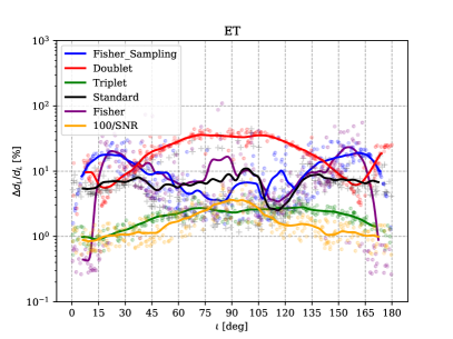
Figure 6: Estimates of $\Delta d_{L}/d_{L}$ vs. $\iota$ averaged over 300 simulations for equal mass, spin-less binary system of fixed total mass $3M_{\odot}$, $d_{L}\simeq 460$ Mpc corresponding to redshift $z=0.1$ in the standard $\Lambda CDM$ model with $H_{0}=70\,km/s/Mpc$ and $\Omega_{M}=0.3$. Cosmological computation makes use of astropy [32].

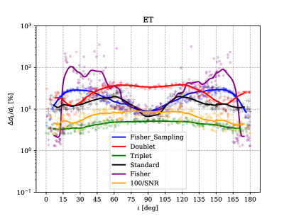
Figure 7: Same as in Fig. 6, but with redshift $z=0.5$, or $d_{L}\simeq 2.8$ Gpc.

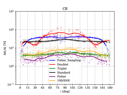
Figure 8: Same as in Fig. 6, but with redshift $z=1$, or $d_{L}\simeq 6.6$ Gpc.

5 Conclusions

We have presented a novel python package for gravitational wave parameter uncertainty forecast based on extending the log-likelihood derivative approximation to higher level than two derivatives. The main scope is to avoid large, unphysical uncertainty forecast for parameters when the Fisher matrix is not invertible.

This software is highly flexible as it allows to call the LAL waveform generator and the stochastic sampling is performed via Bilby. It allows to select an arbitrary detector network by defining detector locations, orientations and topologies.

A crucial step in the calculation of approximate likelihood is derivative computation, so making the precision of numerical derivatives as high as possible is crucial to improve the consistency of the code, which we tested by comparison with results obtained by MonteCarlo sampling of the exact likelihood.

Natural extensions of this code include cosmological applications [33, 34] with assessment of cosmological parameter precision when studying population instead of individual detections.

Appendix A Derivative expansion beyond cubic order: P- and H-Tensors

The Taylor expansion of the likelihood (22) has a 4-th order term specified by the P-Tensor (29):

$$\mathcal{P}_{ijklm} \equiv-\left(\partial_{i}\partial_{j}\partial_{k}\partial_{l}\partial_{m}log\mathcal{L}\right)_{0}$$

$$=-\left[\left\langle\partial_{l}\partial_{m}h|\partial_{i}\partial_{j}\partial_{k}h\right\rangle+(9\ \rm{perms})\right]-\left[\left\langle\partial_{i}h|\partial_{j}\partial_{k}\partial_{l}\partial_{m}h\right\rangle+(4\ {\rm perms})\right]$$

whose contribution to the likelihood is

$$log\mathcal{L}_{5} =-\frac{1}{5!}\sum_{a,\cdots,e}\mathcal{P}_{abcde}\Delta\theta^{abcde}$$

$$=-\sum_{a,\cdots,e}\left[\frac{1}{12}\left\langle\partial_{a}\partial_{b}h|\partial_{c}\partial_{d}\partial_{e}h\right\rangle+\frac{1}{24}\left\langle\partial_{a}h|\partial_{b}\partial_{c}\partial_{d}\partial_{e}h\right\rangle\right]\Delta\theta^{abcde}\,.$$

It contains both 3- and 4- derivative terms, only the former contributing to the Triplet-DALI.

The $H$-Tensor term is

$$\mathcal{H}_{abcdef}\equiv -\left(\partial_{a}\partial_{b}\partial_{c}\partial_{d}\partial_{e}\partial_{f}log\mathcal{L}\right)_{0}$$

$$-\left[\left\langle\partial_{a}\partial_{b}\partial_{c}h|\partial_{d}\partial_{e}\partial_{f}h\right\rangle+(19\ {\rm perms})\right]-\left[\left\langle\partial_{a}\partial_{b}h|\partial_{c}\partial_{d}\partial_{e}\partial_{f}h\right\rangle+(14\ {\rm perms})\right]$$

$$-\left[\left\langle\partial_{a}h|\partial_{b}\partial_{c}\partial_{d}\partial_{e}\partial_{f}h\right\rangle+(5\ {\rm perms})\right]\,,$$

contributing to the likelihood

$$log\mathcal{L}_{6} =-\frac{1}{6!}\sum_{a,\cdots,f}\mathcal{H}_{abcdef}\Delta\theta^{abcdef}$$

$$=-\sum_{a,\cdots,f}\left[\frac{1}{72}\left\langle\partial_{a}\partial_{b}\partial_{c}h|\partial_{d}\partial_{e}\partial_{f}h\right\rangle+\frac{1}{48}\left\langle\partial_{a}\partial_{b}h|\partial_{c}\partial_{d}\partial_{e}\partial_{f}h\right\rangle\right.$$

$$\qquad\qquad\left.+\frac{1}{120}\left\langle\partial_{a}h|\partial_{b}\partial_{c}\partial_{d}\partial_{e}\partial_{f}h\right\rangle\right]\Delta\theta^{abcdef}\,.$$

Collecting the 3-derivative terms from Quarxion, P- and H-tensors we have the Triplet contribution to the likelihood:

$$\left.\log{\cal L}\right|_{Triplet}= -\frac{1}{6}\sum_{a,b,c,d}\left\langle\partial_{a}h|\partial_{b}\partial_{c}\partial_{d}h\right\rangle\Delta\theta^{abcd}-\frac{1}{12}\sum_{a,b,c,d,e}\left\langle\partial_{a}\partial_{b}h|\partial_{c}\partial_{d}\partial_{e}h\right\rangle\Delta\theta^{abcde}$$ (42)

$$-\frac{1}{72}\sum_{a,\dots,f}\left\langle\partial_{a}\partial_{b}\partial_{c}h|\partial_{d}\partial_{e}\partial_{f}h\right\rangle\Delta\theta^{abcdef}$$ (43)

Appendix B Example of parameter recovery

For the analysis of subec. 4.1 we report in Figs. 9,10,11, the relative bias, i.e. the relative difference between the injected and maximum likelihood estimator recovered with different likelihood derivative approximations and with the exact likelihood, running the Nestle [35] MonteCarlo sampler on each of them.

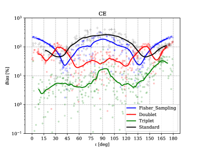
Figure 9: $d_{L}$ relative bias for the same injections as in Fig. 6.

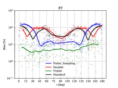
Figure 10: Same as in Fig. 9, but for $z=0.5$ ($d_{L}\simeq 2.8$Gpc).

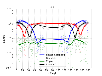
Figure 11: Same as in Fig. 9, but for $z=1$ ($d_{L}\simeq 6.6$Gpc).

References

- [1] R. Abbott, et al., GWTC-3: Compact Binary Coalescences Observed by LIGO and Virgo During the Second Part of the Third Observing Run (11 2021). arXiv:2111.03606.
- [2] J. Aasi, et al., Advanced LIGO, Class. Quant. Grav. 32 (2015) 074001. arXiv:1411.4547, doi:10.1088/0264-9381/32/7/074001.
- [3] F. Acernese, et al., Advanced Virgo: a second-generation interferometric gravitational wave detector, Class. Quant. Grav. 32 (2) (2015) 024001. arXiv:1408.3978, doi:10.1088/0264-9381/32/2/024001.
- [4] T. Akutsu, et al., Overview of KAGRA: Detector design and construction history, PTEP 2021 (5) (2021) 05A101. arXiv:2005.05574, doi:10.1093/ptep/ptaa125.
- [5] Indigo, g-indigo.org.
- [6] M. Maggiore, et al., Science Case for the Einstein Telescope, JCAP 03 (2020) 050. arXiv:1912.02622, doi:10.1088/1475-7516/2020/03/050.
- [7] E. D. Hall, Cosmic Explorer: A Next-Generation Ground-Based Gravitational-Wave Observatory, Galaxies 10 (4) (2022) 90. doi:10.3390/galaxies10040090.
- [8] R. Trotta, Bayes in the sky: Bayesian inference and model selection in cosmology, Contemp. Phys. 49 (2008) 71–104. arXiv:0803.4089, doi:10.1080/00107510802066753.
- [9] S. Borhanian, GWBENCH: a novel Fisher information package for gravitational-wave benchmarking, Class. Quant. Grav. 38 (17) (2021) 175014. arXiv:2010.15202, doi:10.1088/1361-6382/ac1618.
- [10] U. Dupletsa, J. Harms, B. Banerjee, M. Branchesi, B. Goncharov, A. Maselli, A. C. S. Oliveira, S. Ronchini, J. Tissino, gwfish: A simulation software to evaluate parameter-estimation capabilities of gravitational-wave detector networks, Astron. Comput. 42 (2023) 100671. arXiv:2205.02499, doi:10.1016/j.ascom.2022.100671.
- [11] F. Iacovelli, M. Mancarella, S. Foffa, M. Maggiore, GWFAST: A Fisher Information Matrix Python Code for Third-generation Gravitational-wave Detectors, Astrophys. J. Supp. 263 (1) (2022) 2. arXiv:2207.06910, doi:10.3847/1538-4365/ac9129.
- [12] E. Sellentin, M. Quartin, L. Amendola, Breaking the spell of Gaussianity: forecasting with higher order Fisher matrices, Mon. Not. Roy. Astron. Soc. 441 (2) (2014) 1831–1840. arXiv:1401.6892, doi:10.1093/mnras/stu689.
- [13] Z. Wang, C. Liu, J. Zhao, L. Shao, Extending the Fisher Information Matrix in Gravitational-wave Data Analysis, Astrophys. J. 932 (2) (2022) 102. arXiv:2203.02670, doi:10.3847/1538-4357/ac6b99.
- [14] L. Blanchet, Gravitational Radiation from Post-Newtonian Sources and Inspiralling Compact Binaries, Living Rev. Rel. 17 (2014) 2. arXiv:1310.1528, doi:10.12942/lrr-2014-2.
- [15] S. Isoyama, R. Sturani, H. Nakano, Post-Newtonian templates for gravitational waves from compact binary inspirals (12 2020). arXiv:2012.01350, doi:10.1007/978-981-15-4702-7_31-1.
- [16] M. Boyle, et al., The SXS Collaboration catalog of binary black hole simulations, Class. Quant. Grav. 36 (19) (2019) 195006. arXiv:1904.04831, doi:10.1088/1361-6382/ab34e2.
- [17] A. Bohé, et al., Improved effective-one-body model of spinning, nonprecessing binary black holes for the era of gravitational-wave astrophysics with advanced detectors, Phys. Rev. D 95 (4) (2017) 044028. arXiv:1611.03703, doi:10.1103/PhysRevD.95.044028.
- [18] S. Khan, S. Husa, M. Hannam, F. Ohme, M. Pürrer, X. Jiménez Forteza, A. Bohé, Frequency-domain gravitational waves from nonprecessing black-hole binaries. II. A phenomenological model for the advanced detector era, Phys. Rev. D 93 (4) (2016) 044007. arXiv:1508.07253, doi:10.1103/PhysRevD.93.044007.
- [19] LIGO Scientific Collaboration, LIGO Algorithm Library - LALSuite, free software (GPL) (2018). doi:10.7935/GT1W-FZ16.
- [20] P. C. Peters, J. Mathews, Gravitational radiation from point masses in a Keplerian orbit, Phys. Rev. 131 (1963) 435–439. doi:10.1103/PhysRev.131.435.
- [21] L. S. Finn, D. F. Chernoff, Observing binary inspiral in gravitational radiation: One interferometer, Phys. Rev. D 47 (1993) 2198–2219. arXiv:gr-qc/9301003, doi:10.1103/PhysRevD.47.2198.
- [22] B. J. Owen, Search templates for gravitational waves from inspiraling binaries: Choice of template spacing, Phys. Rev. D 53 (1996) 6749–6761. arXiv:gr-qc/9511032, doi:10.1103/PhysRevD.53.6749.
- [23] M. Evans, et al., A Horizon Study for Cosmic Explorer: Science, Observatories, and Community (9 2021). arXiv:2109.09882.
- [24] M. Maggiore, Gravitational Waves. Vol. 1: Theory and Experiments, Oxford University Press, 2007. doi:10.1093/acprof:oso/9780198570745.001.0001.
- [25] L. Blanchet, G. Faye, Q. Henry, F. Larrouturou, D. Trestini, Gravitational Wave Flux and Quadrupole Modes from Quasi-Circular Non-Spinning Compact Binaries to the Fourth Post-Newtonian Order (4 2023). arXiv:2304.11186.
- [26] J. M. S. de Souza, R. Sturani, Luminosity distance uncertainties from gravitational wave detections by third generation observatories (2 2023). arXiv:2302.07749.
- [27] N. D. Lillo, A. Singha, A. Utina, S. Hild, 3g sensitivities and how to look at them, Tech. rep., ET docs (2019).
- [28] V. Srivastava, D. Davis, K. Kuns, P. Landry, S. Ballmer, M. Evans, E. D. Hall, J. Read, B. S. Sathyaprakash, Science-driven Tunable Design of Cosmic Explorer Detectors, Astrophys. J. 931 (1) (2022) 22. arXiv:2201.10668, doi:10.3847/1538-4357/ac5f04.
- [29] B. S. Sathyaprakash, B. F. Schutz, Physics, Astrophysics and Cosmology with Gravitational Waves, Living Rev. Rel. 12 (2009) 2. arXiv:0903.0338, doi:10.12942/lrr-2009-2.
- [30] R. Penrose, A Generalized inverse for matrices, Proc. Cambridge Phil. Soc. 51 (1955) 406–413. doi:10.1017/S0305004100030401.
- [31] G. Ashton, et al., BILBY: A user-friendly Bayesian inference library for gravitational-wave astronomy, Astrophys. J. Suppl. 241 (2) (2019) 27. arXiv:1811.02042, doi:10.3847/1538-4365/ab06fc.
- [32] Astropy Collaboration, A. M. Price-Whelan, P. L. Lim, N. Earl, N. Starkman, L. Bradley, D. L. Shupe, A. A. Patil, L. Corrales, C. E. Brasseur, M. N"othe, A. Donath, E. Tollerud, B. M. Morris, A. Ginsburg, E. Vaher, B. A. Weaver, J. Tocknell, W. Jamieson, M. H. van Kerkwijk, T. P. Robitaille, B. Merry, M. Bachetti, H. M. G"unther, T. L. Aldcroft, J. A. Alvarado-Montes, A. M. Archibald, A. B’odi, S. Bapat, G. Barentsen, J. Baz’an, M. Biswas, M. Boquien, D. J. Burke, D. Cara, M. Cara, K. E. Conroy, S. Conseil, M. W. Craig, R. M. Cross, K. L. Cruz, F. D’Eugenio, N. Dencheva, H. A. R. Devillepoix, J. P. Dietrich, A. D. Eigenbrot, T. Erben, L. Ferreira, D. Foreman-Mackey, R. Fox, N. Freij, S. Garg, R. Geda, L. Glattly, Y. Gondhalekar, K. D. Gordon, D. Grant, P. Greenfield, A. M. Groener, S. Guest, S. Gurovich, R. Handberg, A. Hart, Z. Hatfield-Dodds, D. Homeier, G. Hosseinzadeh, T. Jenness, C. K. Jones, P. Joseph, J. B. Kalmbach, E. Karamehmetoglu, M. Kaluszy’nski, M. S. P. Kelley, N. Kern, W. E. Kerzendorf, E. W. Koch, S. Kulumani, A. Lee, C. Ly, Z. Ma, C. MacBride, J. M. Maljaars, D. Muna, N. A. Murphy, H. Norman, R. O’Steen, K. A. Oman, C. Pacifici, S. Pascual, J. Pascual-Granado, R. R. Patil, G. I. Perren, T. E. Pickering, T. Rastogi, B. R. Roulston, D. F. Ryan, E. S. Rykoff, J. Sabater, P. Sakurikar, J. Salgado, A. Sanghi, N. Saunders, V. Savchenko, L. Schwardt, M. Seifert-Eckert, A. Y. Shih, A. S. Jain, G. Shukla, J. Sick, C. Simpson, S. Singanamalla, L. P. Singer, J. Singhal, M. Sinha, B. M. SipHocz, L. R. Spitler, D. Stansby, O. Streicher, J. Sumak, J. D. Swinbank, D. S. Taranu, N. Tewary, G. R. Tremblay, M. d. Val-Borro, S. J. Van Kooten, Z. Vasovi’c, S. Verma, J. V. de Miranda Cardoso, P. K. G. Williams, T. J. Wilson, B. Winkel, W. M. Wood-Vasey, R. Xue, P. Yoachim, C. Zhang, A. Zonca, Astropy Project Contributors, The Astropy Project: Sustaining and Growing a Community-oriented Open-source Project and the Latest Major Release (v5.0) of the Core Package, apj 935 (2) (2022) 167. arXiv:2206.14220, doi:10.3847/1538-4357/ac7c74.
- [33] R. Gray, et al., Cosmological inference using gravitational wave standard sirens: A mock data analysis, Phys. Rev. D 101 (12) (2020) 122001. arXiv:1908.06050, doi:10.1103/PhysRevD.101.122001.
- [34] R. Gray, C. Messenger, J. Veitch, A pixelated approach to galaxy catalogue incompleteness: improving the dark siren measurement of the Hubble constant, Mon. Not. Roy. Astron. Soc. 512 (1) (2022) 1127–1140. arXiv:2111.04629, doi:10.1093/mnras/stac366.
- [35] P. Mukherjee, D. Parkinson, A. R. Liddle, A nested sampling algorithm for cosmological model selection, Astrophys. J. Lett. 638 (2006) L51–L54. arXiv:astro-ph/0508461, doi:10.1086/501068.