Cubic silicon carbide under tensile pressure: Spinodal instability

Abstract

Silicon carbide is a hard, semiconducting material presenting many polytypes, whose behavior under extreme conditions of pressure and temperature has attracted large interest. Here we study the mechanical properties of $3C$-SiC over a wide range of pressures (compressive and tensile) by means of molecular dynamics simulations, using an effective tight-binding Hamiltonian to describe the interatomic interactions. The accuracy of this procedure has been checked by comparing results at $T=0$ with those derived from ab-initio density-functional-theory calculations. This has allowed us to determine the metastability limits of this material and in particular the spinodal point (where the bulk modulus vanishes) as a function of temperature. At $T=300$ K, the spinodal instability appears for a lattice parameter about 20% larger than that corresponding to ambient pressure. At this temperature, we find a spinodal pressure $P_{s}=-43$ GPa, which becomes less negative as temperature is raised ($P_{s}=-37.9$ GPa at 1500 K). These results pave the way for a deeper understanding of the behavior of crystalline semiconductors in a poorly known region of their phase diagrams.

Keywords: Silicon carbide, negative pressure, molecular dynamics, spinodal line

I Introduction

In the last few decades, the experimentally accessible region of the phase diagrams of different substances has been expanded, giving us deeper understanding of condensed phases under extreme conditions of pressure and temperature.Mujica et al. (2003); Mao et al. (2018) Thus, the effect of hydrostatic pressure on various properties of different types of solids have been largely analyzed. This includes a growing interest in condensed matter under tensile stress, which can yield information on the metastability limits of different phases as well as about the attractive region of interatomic potentials.Davitt et al. (2010); Iyer et al. (2014); Nie et al. (2019); Imre et al. (2008a)

The behavior of condensed matter under hydrostatic tensile pressure has been mainly explored for liquids.Solis and Navarro (1992); Boronat et al. (1994); Jedlovszky and Vallauri (2003); Imre (2007); Imre et al. (2008b); Davitt et al. (2010) This has included the study of the limits for mechanical stability, with the appearance of cavitation close to the corresponding spinodal lines. This kind of phenomena have been also studied for various types of solids, so that extreme pressure conditions do not only refer to large compressive stress, but also to tensile stress (negative pressure).Thakur (1985); Herrero (2003); Iyer et al. (2014); Pei et al. (2015); Liu and Ojamaee (2018); Nie et al. (2019); Verbeeten et al. (2022) It has been shown that tensile pressure can be relevant to understand unexplored regions of stability of solids under hydrostatic (or quasi-hydrostatic) conditions. In this context, one aim of the present paper is to gain insight into the spinodal lines of semiconducting crystalline solids, which delineate the limit of mechanical stability of these materials. These lines are still poorly understood for well-known solids such as Si or silicon carbide. In particular, we concentrate here on cubic $3C$-SiC with zinc-blende-type structure (also called $\beta$ or $B3$ phase).

Silicon carbide under compressive hydrostatic pressure, including phase transitions, has been studied in detail earlier both theoreticallyShimojo et al. (2000); Ramírez et al. (2008); Varshney et al. (2015); Lee and Yao (2015); Ran et al. (2021); Daoud et al. (2022); Pertierra et al. (2022) and experimentally.Zhuravlev et al. (2013); Nisr et al. (2017); Daviau and Lee (2017, 2018); Miozzi et al. (2018); Kim et al. (2022) The interest in the high-pressure behavior of semiconducting materials has recently risen, apart from the traditional context of condensed matter physics, as potential constituents of carbon-rich exoplanets. Various studies have found that high pressure in planetary interiors may significantly change the physical properties of these materials.Nisr et al. (2017); Miozzi et al. (2018); Kim et al. (2022)

Given the large amount of work carried out for $3C$-SiC under compressive pressure, we focus here mainly on the effects of tensile stress. In this context, crystalline silicon has been investigated at negative pressure by molecular dynamics simulations, yielding information on the appearance of cavitation and crystal-liquid interfaces,Wilson and McMillan (2003); Daisenberger et al. (2010) as well as on the transition from diamond-type structure to a clathrate at a pressure $P\approx-2.5$ GPa.Kaczmarski et al. (2005)

The experimentally reachable range of hydrostatic (or quasi-hydrostatic) tensile pressure has been growing along the years, as well as the understanding of physical properties under conditions hardly accessible in the laboratory.Davitt et al. (2010); Henderson and Speedy (1987); Grade (1988); Moshe et al. (2000); Dunstan et al. (2002); Verbeeten et al. (2022) Detailed quantitative experimental studies of materials under negative pressure are scarce as one works in metastable conditions, which in many cases are only available for short periods of time. In our present context, carbon-based materials have been studied under tensile pressure by means of ultrasonic cavitation and shock waves created by picosecond laser pulses.Abrosimov et al. (2014); Khachatryan et al. (2008) Moreover, low-density clathrates, allotropes of group IVa elements (C, Si, Ge), which turn out to be metastable at ambient conditions, have been synthesized in recent years.Baranowski et al. (2014); Guloy et al. (2006)

In this paper we explore the metastability region of cubic SiC under tensile hydrostatic pressure. We present results of molecular dynamics (MD) simulations carried out using interatomic interactions based on a reliable tight-binding (TB) Hamiltonian. Density-functional-theory (DFT) calculations were performed at $T=0$ to assess the precision of the TB results for conditions (crystal volume) far from equilibrium. We find that $3C$-SiC is metastable in a wide pressure range till $P\sim-40$ GPa, and MD simulations allow us to approach the limit of mechanical stability of the solid (spinodal pressure), which is obtained at temperatures up to 1500 K.

The paper is organized as follows. In Sec. II we present the computational methods used in the calculations. In Sec. III we show the phonon dispersion bands and the elastic constants of $3C$-SiC. Results for the energy obtained from TB and DFT methods are given in Sec. IV. The spinodal instability appearing at negative pressures is discussed in Sec. V, and a summary of the main results is presented in Sec. VI.

II Computational method

In this section we present the methods used in this paper. In Sec. II.A we concentrate on molecular dynamics simulations and the tight-binding procedure employed to define the interatomic interactions. In Sec. II.B, we introduce the DFT-based approach employed to evaluate the accuracy of the TB results at $T=0$.

II.1 Tight-binding molecular dynamics

We investigate structural and mechanical properties of $3C$-SiC as functions of temperature and pressure using MD simulations. A relevant point in the MD method is the consideration of realistic interatomic interactions, which should be as reliable as possible. One could achieve this goal by employing ab-initio density functional or Hartree-Fock based self-consistent potentials for finite-temperature simulations, but this would enormously limit the length of the simulation trajectories which could be obtained in a reasonable computing time. We then determine the interatomic forces from an effective tight-binding Hamiltonian, built up from results of density functional calculations.Porezag et al. (1995)

This type of TB methods display good accuracy to describe several properties of condensed matter and molecular systems, as discussed by Goringe et al.Goringe et al. (1997) and Colombo.Colombo (2005) The TB Hamiltonian used herePorezag et al. (1995) was found before to be trustworthy to define the interatomic interactions in carbon-based materials.Herrero et al. (2006); Herrero and Ramírez (2007) The parametrization for structures containing Si and C atoms was given in Ref. Gutierrez et al., 1996. The non-orthogonality of the atomic basis is a crucial clue for the transferability of the parametrization to complex systems Porezag et al. (1995).

The tight-binding method was employed earlier to study silicon carbide, especially the cubic phase considered here.Mercer (1996); Bernstein et al. (2005) In particular, the TB Hamiltonian used in this work has been applied before to study reconstructions of $3C$-SiC surfaces,Gutierrez et al. (1996); Shevlin et al. (2001) as well as to investigate isotopic and nuclear quantum effects in this material.Ramírez et al. (2008); Herrero et al. (2009) In relation with our present work, it was employed to study this crystalline solid under compressive pressure up to 60 GPa, with results that compared well with experimental data and other theoretical calculations.Ramírez et al. (2008) More recently, this TB model has been applied to analyze several properties of the lately synthesized monolayers of silicon carbide.Herrero and Ramírez (2022); Polley et al. (2023)

TB MD simulations have been carried out in the isothermal-isobaric ($NPT$) ensemble for cubic SiC supercells including 64 and 216 atoms. Some simulations were performed in the canonical ($NVT$) ensemble near the limit of mechanical stability, as they allow to perform simulations closer to the spinodal point, in a region where $NPT$ simulations are unstable due to the appearance of large volume fluctuations. Periodic boundary conditions were assumed in all cases.

To keep the required temperature, chains of four Nosé-Hoover thermostats were coupled to each atomic degree of freedom.Tuckerman and Hughes (1998) For $NPT$ simulations, an additional chain of four thermostats was connected to the barostat that controls the volume of the simulation cell, giving a constant pressure.Tuckerman and Hughes (1998); Allen and Tildesley (1987) The equations of motion were integrated by employing the reversible reference system propagator algorithm (RESPA), which permits to use different time steps for the integration of slow and fast degrees of freedom.Martyna et al. (1996) The time step $\Delta t$ employed for the dynamics associated to the forces derived from the TB Hamiltonian was 1 fs, which gives good accuracy for the temperatures studied here. For fast dynamical variables such as the thermostats, we used a time step $\delta t=0.25$ fs. The configuration space has been sampled for temperatures from 300 to 1500 K. Given a temperature, a typical run consisted of $2\times 10^{5}$ MD steps for system equilibration, and $8\times 10^{6}$ steps for the calculation of mean variables.

For sampling electronic degrees of freedom in the reciprocal space, we have considered only the $\Gamma$ point (${\bf k}=0$). The main consequence of employing larger ${\bf k}$ sets is a shift of the total energy, with imperceptible change in energy differences between various atomic configurations. Something similar occurs for the mean energy per atom at a given temperature, for different cell sizes.Herrero and Ramírez (2022) This has been checked here for silicon carbide using simulation cells of size $N$ = 64 and 216 atoms.

We calculate the elastic constants of cubic SiC at finite temperatures by applying a particular component of the stress tensor $\{\tau_{ij}\}$ in isothermal-isobaric simulations, and finding the compliance constants $S_{ij}$ from the obtained strain. For instance, for $\tau_{xx}\neq 0$ and $\tau_{ij}=0$ for the other components, we have $S_{11}=e_{xx}/\tau_{xx}$, and $S_{12}=e_{yy}/\tau_{xx}$, $e_{ij}$ being the components of the strain tensor.Ashcroft and Mermin (1976); Kittel (2005); Yu and Cardona (1996) From the compliance constants, we obtain the stiffness constants $C_{11}$ and $C_{12}$ by means of the relations corresponding to cubic crystals:Ashcroft and Mermin (1976); Kittel (2005) $C_{11}=(S_{11}+S_{12})/Z$ and $C_{12}=-S_{12}/Z$, with

$$Z=(S_{11}-S_{12})(S_{11}+2S_{12})\;.$$ (1)

Note that a hydrostatic pressure $P$ corresponds in the elasticity notation to $\tau_{xx}=\tau_{yy}=\tau_{zz}=-P$. Here, $P>0$ and $P<0$ represent compressive and tensile pressure, respectively.

II.2 DFT calculations

In order to verify the accuracy of our TB method for describing the mechanical properties of cubic SiC, we have performed state-of-the-art DFT calculations. Total energies were obtained with the Quantum-ESPRESSO package for electronic structure calculations.Giannozzi et al. (2009, 2017) We employed the Perdew-Burke-Ernzerhof exchange-correlation functional, as adapted for solids (PBEsol),Perdew et al. (2008) using a plane wave basis set with a kinetic energy cutoff of 45 Ry (400 Ry for the charge density cutoff). Projector-augmented-wave (PAW) pseudopotentials were employed for both carbon and silicon.sc- We considered a cubic cell of SiC containing 8 atoms with zinc-blende structure, subject to periodic boundary conditions. The Brillouin zone was integrated with a $10\times 10\times 10$ Monkhorst-Pack grid.Monkhorst and Pack (1976)

Ab-initio calculations were carried out earlier to study several aspects of $3C$-SiC, such as structural, electronic, elastic, lattice-dynamical, and thermodynamic properties.Churcher et al. (1986); Park et al. (1994); Karch et al. (1994); Kackell et al. (1994); Cannuccia and Gali (2020) In the context of our present work, they have been employed to characterize phase transitions in this material under high pressure.Chang and Cohen (1987); Lee and Yao (2015); Kidokoro et al. (2017); Shahi et al. (2018); Ran et al. (2021)

III Energy

In Fig. 1 we present the energy per atom as a function of the lattice parameter $a$ of $3C$ silicon carbide. The solid line represents results of PBEsol-PAW DFT calculations. We find for the minimum-energy configuration a lattice parameter $a_{0}$ = 4.358 Å, in agreement with the result of Lee and Yao.Lee and Yao (2015) Note that the zero of energy is taken at $a_{0}$. The dashed line corresponds to our tight-binding calculations at $T=0$. It displays a minimum at $a_{0}$ = 4.346 Å, and follows closely the DFT result for lattice parameters around $a_{0}$. For large values of $a$, in the region where the material becomes unstable, both lines progressively depart from one another, the TB energy being higher than that corresponding to the DFT calculations, and for $a=$ 5.5 Å the difference between both amounts to 0.17 eV.

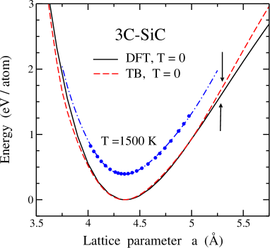
Figure 1: Energy vs lattice parameter $a$ of $3C$ silicon carbide. The solid and dashed lines represent results of DFT and TB calculations at $T=0$. Solid circles indicate results of MD simulations at $T=1500$ K. The dashed-dotted line corresponds to an upwards shift of the $T=0$ TB line by an amount of $3k_{B}T$ for 1500 K. Error bars of the simulation data are less than the symbol size. Two vertical arrows show the inflection points of the solid and dashed curves.

At $T=0$, the hydrostatic pressure is given by $P=-\partial E/\partial V$. Thus, for the TB model, the pressure $P$ corresponding to lattice parameter $a$ from 3.7 to 5.25 Å goes from 303 to $-44$ GPa. Note that the range of lattice parameters that are explored with compressive pressure ($P>0$) up to about 300 GPa corresponds to a reduction of $a$ by a 15%. On the contrary, tensile pressure causes expansion of the lattice with an increase in $a$ by a 21% up to the stability limit for $P\approx-44$ GPa.

To show the effect of temperature, we also display in Fig. 1 results of MD simulations at $T=1500$ K (solid circles). These data were obtained from simulations in the isothermal-isobaric $NPT$ ensemble for hydrostatic pressures between 80 GPa ($a$ = 4.02 Å) and $-37.3$ GPa ($a$ = 4.97 Å). Note that the latter pressure is near the spinodal pressure $P_{s}$, where the solid becomes unstable at $T=1500$ K (see below). At this pressure and temperature we find in the MD simulations an energy $E$ = 1.28 eV/atom. This energy can be split into a contribution of 0.89 eV/atom due to elastic energy (lattice expansion) and another of 0.39 eV/atom due to thermal energy, $E_{\rm th}$, at this temperature. This means that at this relatively high temperature, $E_{\rm th}$ represents a 30% of the total energy close to the spinodal pressure $P_{s}$.

For comparison with the simulation results at $T$ = 1500 K, we present in Fig. 1 the expected energy for a classical harmonic model for the lattice vibrations at each crystal volume at this temperature (dashed-dotted curve). This is obtained by adding an energy of $3k_{B}T$ ($k_{B}$, Boltzmann’s constant) to the zero-temperature TB result. One observes that both finite-temperature data sets follow each other closely.

For our later discussion on the mechanical stability of $3C$-SiC, it is interesting to determine the inflection point of the curves displayed in Fig. 1. This point separates the regions where they are concave upward ($d^{2}E/da^{2}>0$) and downward ($d^{2}E/da^{2}<0$), and is represented by vertical arrows for the $T=0$ curves in Fig. 1.

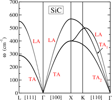
Figure 2: Acoustic phonon bands of $3C$-SiC derived from the dynamical matrix corresponding to the tight-binding model for the minimum-energy volume. Labels indicate the character of the different branches: LA, longitudinal acoustic; TA, transversal acoustic. The TA band along $[111]$ and $[100]$ directions is twofold degenerate.

IV Phonon dispersion bands and elastic constants

The elastic stiffness constants $C_{ij}$ of cubic SiC calculated with the TB Hamiltonian for $T=0$ may be taken as a reference for the finite-temperature analysis presented below. We obtain these elastic constants in the low-$T$ limit from the harmonic dispersion relation of acoustic phonons. To define the dynamical matrix necessary to find the phonon bands, we calculated the interatomic force constants by numerical differentiation of atomic forces, taking atom displacements of $2\times 10^{-4}$ Å from the minimum-energy sites. Good numerical convergence in the phonon bands was achieved by calculating all interatomic force constants up to distances of about 18 Å. In Fig. 2 we present the acoustic phonon branches obtained in this way for the minimum-energy configuration ($a_{0}=4.346$ Å), along symmetry directions of the Brillouin zone. The phonon dispersion displayed in this plot is similar to those found for other effective potentials and DFT calculations,Karch et al. (1994); Talwar (2017); Wang et al. (2017); Bartolomei et al. (2021) and to the acoustic phonon bands obtained from inelastic x-ray scattering.Serrano et al. (2002)

The sound velocities for the acoustic bands along the directions shown in Fig. 2 are given by the slope of the bands at the $\Gamma$ point ($k\to 0$). Here $k$ denotes the wavenumber, i.e., $k=|{\bf k}|$, and ${\bf k}=(k_{x},k_{y},k_{z})$ is a wavevector in the Brillouin zone. The elastic constants $C_{11}$ and $C_{12}$, relevant for our discussion on the bulk modulus and the mechanical stability of the solid, can be calculated from the expressions:Kittel (2005); Yu and Cardona (1996)

$$C_{11}=\rho\left(\frac{\partial\omega_{\rm LA}}{\partial k_{x}}\right)^{2}_{\Gamma}\;,$$ (2)

for the LA band along the $[100]$ direction, and

$$C_{12}=C_{11}-2\rho\left(\frac{\partial\omega_{\rm TA_{2}}}{\partial k}\right)^{2}_{\Gamma}\;.$$ (3)

for the TA₂ band along the $[110]$ direction. Here $\rho$ is the density of the solid. From the phonon bands shown in Fig. 2, using Eqs. (2) and (3), we find $C_{11}$ = 452.9 GPa and $C_{12}$ = 141.1 GPa. We have checked the consistency of these values with those obtained from the slopes of the different bands at the $\Gamma$ point along the directions in ${\bf k}$-space shown in this figure.

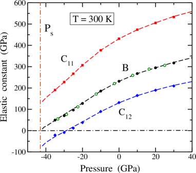
Figure 3: Pressure dependence of the elastic constants $C_{11}$ (squares) and $C_{12}$ (diamonds) derived from MD simulations of $3C$-SiC at $T=$ 300 K. Solid circles represent the bulk modulus $B$ obtained from the elastic constants by using Eq. (4). Open circles indicate values of $B$ found from numerical differentiation of the $P-V$ curve. Error bars are in the order of the symbol size. The vertical dashed-dotted line shows the spinodal pressure at 300 K. Dashed lines are guides to the eye.

At finite temperatures, we have calculated the stiffness constants $C_{11}$ and $C_{12}$ from MD simulations as indicated above in Sec. II.A. For stress-free silicon carbide, we find an appreciable decrease in both elastic constants for rising temperature. Thus, at $T$ = 300 K we have $C_{11}=$ 434.8 GPa and $C_{12}=$ 129.4 GPa, which means a reduction of 4% and 8%, respectively, with respect to the zero-temperature values. At the highest temperature considered here, $T=1500$ K, we find a decrease of 15% and 26%, respectively, in comparison with the $T=0$ values.

In Fig. 3 we show the dependence of $C_{11}$ and $C_{12}$ on hydrostatic pressure $P$ at 300 K. Symbols represent data derived from our MD simulations. For positive (compressive) $P$, we observe an increase of both elastic constants. For increasing tensile (negative) pressure, the elastic constants decrease, and at $P=-27$ GPa, $C_{12}$ becomes negative. Note that $C_{11}>0$ in the considered pressure range, as this is a condition for mechanical stability of a solid phase.Jamal et al. (2014); Mouhat and Coudert (2014)

An important characteristic of solids concerning their elastic properties is the Poisson’s ratio $\nu$, which may be expressed for a cubic phase as $\nu=C_{12}/C_{11}$. Thus we have in the classical low-temperature limit $\nu$ = 0.31. This parameter changes for rising temperature, as the elastic constants, and for ambient conditions ($T$ = 300 K, $P$ = 0) we find $\nu=0.30$, close to a value $\nu=0.31(1)$ derived by Zhuravlev et al. from x-ray diffraction and Brillouin spectroscopy.Zhuravlev et al. (2013) At 300 K, the Poisson’s ratio yielded by our MD simulations becomes negative as $C_{12}$ for $P=-27$ GPa, and cubic SiC transforms into an auxetic solid at this tensile pressure.

The isothermal bulk modulus, defined as $B=-V\,\partial P/\partial V$, can be obtained from the elastic constants by means of the expression, valid for cubic crystals:Ashcroft and Mermin (1976); Kittel (2005); Jamal et al. (2014)

$$B=\frac{1}{3}(C_{11}+2C_{12})\;.$$ (4)

From the elastic constants given above, we obtain at $T=0$: $B_{0}$ = 245.0 GPa. We estimate an error bar of $\pm 2$ GPa, mainly caused by the uncertainty in the determination of the phonon band slopes at the $\Gamma$ point. The classical zero-temperature bulk modulus can be also obtained as

$$B_{0}=V_{0}\left.\frac{\partial^{2}E}{\partial V^{2}}\right|_{V_{0}}\;,$$ (5)

where $E$ is the energy and $V_{0}$ is the volume for the minimum-energy configuration. This gives for our TB Hamiltonian $B_{0}$ = 245.6 GPa, which agrees with the value calculated from the elastic constants, taking into account the error bars.

From the elastic constants, we find (using Eq. (4)) at $T=300$ K and $P=0$ a bulk modulus $B$ = 232(1) GPa, to be compared with experimental resultsAleksandrov et al. (1989); Strossner et al. (1987); Wang et al. (2016) in the range from 224 GPaYean and Riter (1971) to 260 GPa.Yoshida et al. (1993) Our value for 300 K means a reduction of about a 6% with respect to the zero-temperature result. According to the data found for $C_{11}$ and $C_{12}$, we have for $T=1500$ K a bulk modulus $B$ = 198(1) GPa. From the decrease in $B$ for rising $T$, we obtain around room temperature ($T$ = 300 K) a derivative $\partial B/\partial T=-0.040(2)$ GPa K^-1, close to the value derived by Wang et al.Wang et al. (2016) from x-ray diffraction experiments: $\partial B/\partial T=-0.037(4)$ GPa K^-1.

The modulus $B$ is especially interesting to study the critical behavior of silicon carbide under hydrostatic pressure. In Fig. 3 we display, along with the elastic constants, the dependence of $B$ on $P$ at $T=300$ K, including tensile and compressive pressure. Solid circles indicate values of $B$ obtained from the elastic constants using Eq. (4). For comparison we also display as open circles results for $B$ obtained from numerical differentiation of the $P-V$ equation of state at this temperature, using the expression $B=-V\,\partial P/\partial V$. Results of both procedures agree well in the whole pressure region shown in Fig. 3 (error bars are in the order of the symbol size), which gives a consistency check for our calculations.

V Spinodal instability

The material dilation due to tensile stress causes a fast decrease in the bulk modulus $B$, which vanishes for a pressure $P_{s}$, where SiC becomes mechanically unstable. This is typical of a spinodal point in the $(P,T)$ phase diagram.Sciortino et al. (1995); Herrero (2003); Ramírez and Herrero (2018); Callen (1985) For a given temperature $T$, there is a range of tensile pressure where cubic SiC is metastable, i.e., for $0>P>P_{s}$. The spinodal line, which delineates the unstable phase ($P<P_{s}$) from the metastable phase, is the locus of points $P_{s}(T)$ where $B=0$. This type of spinodal lines have been investigated before for water,Speedy (1982) as well as for ice, SiO₂ cristobalite,Sciortino et al. (1995) and noble-gas solidsHerrero (2003) close to their stability limits. In the last few years, this question has been considered for two-dimensional materials, in particular for graphene, where this kind of instability appears also for compressive stress.Ramírez and Herrero (2018, 2020)

V.1 Isothermal formulation

Close to a spinodal point, the Helmholtz free energy for temperature $T$ can be written as a Taylor power expansion in terms of $V_{s}-V$:Speedy (1982); Boronat et al. (1994); Ramírez and Herrero (2020)

$$F(V,T)=F(V_{s}(T),T)+a_{1}(T)\,[V_{s}(T)-V]+$$

$$a_{3}(T)\,[V_{s}(T)-V]^{3}+...\;,$$ (6)

where $V_{s}(T)$ and $F(V_{s}(T),T)$ are the volume and free energy at the spinodal point. At this point one has $\partial^{2}F/\partial V^{2}=0$, so that a quadratic term does not appear on the r.h.s of Eq. (6), i.e., $a_{2}=0$. Note that the coefficients $a_{i}$, as well as the spinodal volume $V_{s}$, are in general dependent on the temperature. In the following we will not write this dependence explicitly.

The pressure is

$$P=-\frac{\partial F}{\partial V}=P_{s}+3a_{3}\,(V_{s}-V)^{2}+...\;,$$ (7)

and $P_{s}=a_{1}$ is the spinodal pressure, which corresponds to the volume $V_{s}$. The isothermal bulk modulus is given by

$$B=V\,\frac{\partial^{2}F}{\partial V^{2}}=-V\,\frac{\partial P}{\partial V}\;,$$ (8)

and to leading order in an expansion in powers of $V_{s}-V$, we have

$$B=6a_{3}V_{s}(V_{s}-V)\;,$$ (9)

or considering Eq. (7), $B$ can be expressed along an isotherm, close to the spinodal pressure $P_{s}$, as

$$B=2\sqrt{3a_{3}}\,V_{s}\,(P-P_{s})^{1/2}\;.$$ (10)

Thus, the bulk modulus vanishes for $P=P_{s}$, which gives the limit of mechanical stability for the considered phase.

In the present work, most of the simulations have been carried out in the isothermal-isobaric ensemble, and we determine $P_{s}$ as a function of $T$. Similarly, for a given volume $V$, there are spinodal pressure $P_{s}(V)$ and temperature $T_{s}(V)$, and changing $P$ and $T$ along an isochore close to the spinodal point, one has to first order the linear relation $P-P_{s}(V)\propto T-T_{s}(V)$.Speedy (1982)

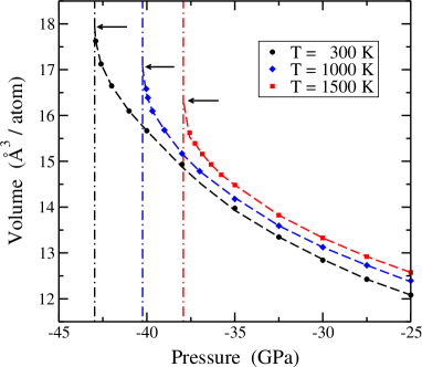
Figure 4: Pressure dependence of the volume of cubic SiC, as derived from MD simulations at $T$ = 300 K (circles), 1000 K (diamonds), and 1500 K (squares). Vertical dashed-dotted lines indicate the spinodal pressure for each temperature. Arrows show the spinodal volume in each case. Error bars of the simulation data are in the order of the symbol size. Dashed curves are guides to the eye.

V.2 Application to $3C$-SiC

In Fig. 4 we display the pressure dependence of the volume of cubic SiC for $T$ = 300, 1000, and 1500 K. Solid symbols represent results of MD simulations at various tensile pressures. For each temperature, one observes an increase in volume for rising tensile pressure ($P$ more negative), i.e., $dV/dP<0$, as required for thermodynamic consistency. At a certain pressure (spinodal) $dV/dP$ diverges to $-\infty$. Note that the slope of each $P-V$ curve shown in Fig. 4 diverges for a spinodal volume $V_{s}(T)$, shown by a horizontal arrow. The corresponding spinodal pressures $P_{s}(T)$ are indicated by vertical dashed lines at $P_{s}=-43.0,-40.2$ and $-37.9$ GPa for $T$ = 300, 1000, and 1500 K, respectively.

The large volume fluctuations appearing in $NPT$ simulations close to the spinodal pressure do not allow us to reliably sample that region of the configuration space. This limitation increases as the temperature is raised and the volume fluctuations also rise. This problem is remedied in part by carrying out canonical ($NVT$) simulations in those parts of the configuration space, where $3C$-SiC remains metastable during simulation runs long enough to accurately sample the required thermodynamic variables.

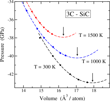
Figure 5: Pressure vs volume for $3C$-SiC at $T$ = 300 K (circles), 1000 K (diamonds), and 1500 K (squares), derived from MD simulations. Error bars are in the order of the symbol size. The dashed lines are parabolic fits to the data points. Arrows indicate the spinodal volume for each temperature.

To define the spinodal volume, $V_{s}$, and pressure, $P_{s}$, we have carried out for each considered temperature a fit of our data close to the spinodal instability to the expression $P=P_{s}+c(V_{s}-V)^{2}$ [see Eq. (7), with $c=3a_{3}$]. In Fig. 5 we show the fits corresponding to $T$ = 300, 1000, and 1500 K. In each of these fits we considered the five data points nearest to the instability. In this figure, arrows indicate the spinodal volumes for the given temperatures. Following this procedure, we have obtained $P_{s}$ and $V_{s}$ for several temperatures in the range from 300 to 1500 K.

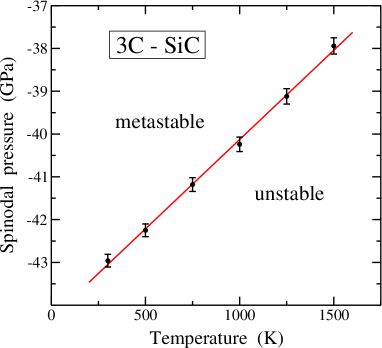
Figure 6: Calculated spinodal pressure for $3C$-SiC as a function of temperature. Solid circles are data points derived from MD simulations. The solid line is a least-square fit to the data points, showing the separation between regions of metastability and mechanical instability for $3C$-SiC.

In Fig. 6 we present the temperature dependence of the spinodal pressure of $3C$-SiC, as derived from our MD simulations (solid symbols). The solid line is a fit to the data points: $P_{s}=b_{1}+b_{2}T$, with $b_{1}=-44.3$ GPa and $b_{2}=4.2$ MPa/K. The solid is metastable at negative pressures in the region above the line in Fig. 6. Below the line it is mechanically unstable, so that in this region it transforms into the gas phase, and the volume diverges to infinity under tensile pressure. When approaching the line from the metastable region, the transition may happen well before arriving at the spinodal, as occurs in our isothermal-isobaric MD simulations when increasing the tensile stress or the temperature.

For comparison with the finite-temperature data obtained with the TB model, we have calculated the spinodal pressure at $T=0$ from DFT calculations. In this case, we obtain the pressure as $P=-\partial E/\partial V$, and $P_{s}$ is given by the condition $\partial P/\partial V=0$. We find $P_{s}=-39$ GPa, which means that the tight-binding method overestimates the spinodal pressure by about a 10%.

Up to now, we have studied the dependence of the spinodal pressure on the temperature. Conversely, one can consider the temperature at which the solid becomes unstable as a function of the crystal volume. These results are summarized in Fig. 7, where we display the spinodal temperature vs. the volume $V$. Solid circles are data points derived from fits of the $P-V$ curves yielded by MD simulations to the expression in Eq. (7). Error bars in the volume are associated to the uncertainty in the spinodal volume derived in the corresponding fits, as those shown in Fig. 5. A linear fit to the points in Fig. 7 yields a slope $dT_{s}/dV=-704$ K/ų, and extrapolates at $T=0$ to a volume $V=18.4$ Å³/atom. This corresponds to a lattice parameter $a$ = 5.28 Å, consistent with calculations based on the zero-temperature energy curve shown in Fig. 1 (dashed line), where the inflection point is indicated by a vertical arrow.

All the results presented here correspond to classical calculations and MD simulations. This means that nuclear quantum effects, which should appear at low temperatures are not taken into account. Thus, the low-$T$ limit, which is presented here as a reference for finite temperature results correspond to the classical limit, and does not take into account quantum corrections as those arising from atomic zero-point motion. An analysis of low-temperature quantum corrections to the results presented here is out of the scope of the present paper, and could be analyzed by means of path-integral simulations, as those employed earlier to study spinodal instabilities in noble-gas solids.Herrero (2003)

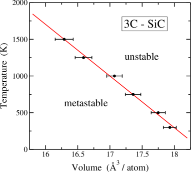
Figure 7: Spinodal temperature vs volume for $3C$-SiC, as derived from MD simulations (solid circles). The line is a least-square fit to the data points. In the regions below and above the line cubic silicon carbide is metastable and mechanically unstable, respectively.

VI Summary

In this paper we have presented and discussed results of MD simulations of cubic silicon carbide in a large range of temperature and pressure. This method has permitted us to quantify structural and elastic properties of this crystalline semiconductor, with particular emphasis upon its limit of mechanical stability.

We have concentrated on the elastic constants and the region of mechanical stability under tensile pressure. With this purpose, we have put forth the results of extensive simulations of this material using a well-checked tight-binding Hamiltonian, for a wide range of temperatures and hydrostatic pressures. The results of our MD simulations have been found to be consistent with DFT calculations at $T=0$ in a large range of crystal volumes and pressures. This has served us as a check for the precision of the TB Hamiltonian employed here to study silicon carbide for crystal volumes far from the equilibrium state at ambient conditions.

For $P=0$, the elastic constants $C_{11}$ and $C_{12}$ of cubic SiC, as well as the Poisson’s ratio $\nu$, are found to decrease for rising temperature, as discussed in Sec. IV. This decrease is even more important in the presence of tensile stress, so that at $T$ = 300 K, $C_{12}$ and $\nu$ become negative for a pressure $P=-27$ GPa ($3C$-SiC converts into an auxetic material). For larger negative pressure, one reaches the spinodal instability, where the solid becomes mechanically unstable (vanishing bulk modulus). For $T=300$ K, this happens at $P_{s}=-43$ GPa, a spinodal pressure which is less negative for higher $T$: $P_{s}=-37.9$ GPa at 1500 K.

The computational approach presented in this paper has proven to be a reliable tool to describe the effect of pressure in metastable states in solids. In particular, it allows to determine the spinodal line under tensile stress as a function of temperature. Further work in this subject is necessary to generalize the results presented here to other related crystalline materials, for which the stability limits are expected to depend on their elastic properties. This can be realized by means of atomistic simulations using accurate tight-binding Hamiltonians as that employed here for SiC.

Data availability

The data that support the findings of this study are available from the corresponding author upon reasonable request.

CRediT author contribution statement

Carlos P. Herrero: Data curation, Investigation, Validation, Original draft

Rafael Ramírez: Methodology, Software, Investigation, Validation

Gabriela Herrero-Saboya: Methodology, Investigation, Validation

Declaration of Competing Interest

The authors declare that they have no known competing financial interests or personal relationships that could have appeared to influence the work reported in this paper.