Role of positional disorder in fully textured ensembles of Ising-like dipoles

Abstract

We study by numerical simulation the magnetic order in ensembles of randomly packed magnetic spherical particles which, induced by their uniaxial anisotropy in the strong coupling limit, behave as Ising dipoles. We explore the role of the frozen disorder in the positions of the particles assuming a common fixed direction for the easy axes of all spheres. We look at two types of spatially disordered configurations. In the first one we consider isotropic positional distributions which can be obtained from the liquid state of the hard sphere fluid. We derive the phase diagram in the $T$-$\Phi$ plane where $T$ is the temperature and $\Phi$ the volume fraction. This diagram exhibits long-range ferromagnetic order at low $T$ for volume fractions above the threshold $\Phi_{c}=0.157$ predicted by mean-field calculations. For $\Phi\lesssim\Phi_{c}$ a spin-glass phase forms with the same marginal behavior found for other strongly disordered dipolar systems. The second type of spatial configurations we study are anisotropic distributions that can be obtained by freezing a dipolar hard sphere liquid in its polarized state at low temperature. This structural anisotropy enhances the ferromagnetic order present in isotropic hard sphere configurations.

I INTRODUCTION

Advances in nanotechnology have permitted to synthesize nanoparticles (NP) of various sizes and shapes, with or without non-magnetic coating layers, and to create monodisperse systems of NP with a certain control on their spatial distribution.nano Small enough NP (with diameters of about 10-30 nm) have a single domain that behaves like a magnetic dipole.skomski

Furthermore the internal structure of the NP gives rise to the magnetocrystalline anisotropy energy (MAE) tending to orient the dipoles along local easy axes. Under such a circumstance magnetic spin flips have a non-vanishing energetic cost $E_{a}$.bedanta ; fiorani For sufficiently dense packings, the interaction energy $E_{dd}$ between nearby dipoles can be comparable to $E_{a}$. For example for compact packings of bare maghemite nanoparticles the ratio $E_{a}/E_{dd}$ is approximatelysmall $E_{a}/E_{dd}\approx 6$. For such systems $E_{dd}$ can induce complex collective behavior endowing them with a rich phenomenology, mainly at low temperature.fiorani ; toro1 ; sawako . Indeed, the spatial variations of the dipolar fields lead to geometric frustration, making these systems rather sensitive to the relative positions and directions of their dipoles. For example, dipoles placed in well-ordered crystalline arrangements exhibit ferro- (FM) or antiferromagnetic (AF) order depending on the lattice geometry. luttinger

In the strong MAE limit the dipole of each NP points up or down nearly parallel to its local easy axis leading to a dipolar Ising-like model knak where only $E_{dd}$ play a central role.

The study of the magnetic order in systems of magnetic NP is an active field of research.bookpeddis ; batlle Its interest ranges from fundamental physics, because of the need of understanding the collective effects of samples of NP, to their applications into a broad class of technological problems like data storagedobson or nanomedicine.medicine

When the arrangements of NP are obtained by freezing the carrier fluid in colloidal suspensions of NP,ferrofluids or by compacting powders of granular solids,powder disorder both in dipole orientations and in position result. This double disorder along with the geometric frustration inherent to dipolar interactions may give rise to dipolar spin-glass behavior. This has been observed experimentally in frozen ferrofluids,ferrofluids ; morup and in pressed powders of NP.powder ; toro1

The role played by the orientational disorder (called texturation) has been studied by Monte Carlo simulations in crystaline latticesrussier20 and in random distributions.alonso19 In both cases the magnetic order at low temperature changed from FM to spin-glass (SG) as the orientational disorder increased from textured (parallel axis dipoles) to non–textured (random axis dipoles). The same has been found in non-textured systems by using the ratio $E_{a}/E_{dd}$ as disorder parameter.russier20b

On the other hand, the role played by the disorder in positions in systems of NP is not completely understood. Heisenberg dipoles with no local anisotropies placed in random dense packings (RDP) have been studied by Monte Carlo simulations. Given that the dipoles can rotate freely, the frozen disorder is only in positions and depends on the fraction $\Phi$ of volume occupied by the NP. Numerical simulations find FM order for $\Phi\gtrsim 0.49$ and SG order otherwise.alonso20 In the mean-field approach, Zhang and Widom found FM order for $\Phi\geq 0.295$ under the crude approximation of $g(r)=1$ where $g(r)$ is the radial distribution function.zhang This discrepancy seems to be due to the spatial correlations at short distances for RDP.

Reverting to systems of NP, it must be noticed that the local anisotropy in single domain NP is always non-zero. For this reason, the only way to suppress orientational disorder in such systems in order to explore only positional disorder effects, is to consider textured systems. It has been recently found that the alignment of the easy-axes reduces the dipolar field acting on each NP for volume fractions $0.3\lesssim\Phi$.moya A certain texturation arises naturally in colloidal liquids even in absence of an external field. Even for moderate values of the volume fraction ($0.25\lesssim\Phi\lesssim 0.5$), the dipolar hard sphere (DHS) fluid polarizes for temperatures below the ferromagnetic transition temperature exhibiting anisotropic short ranged spatial correlations.weis ; weis2 ; malherbe23

In this paper we investigate the magnetic order of systems of textured dipoles as a function of the positional disorder in RDP. For this purpose we will use Ising dipoles that point up and down along a common direction such that the structural disorder comes only from the spatial distribution. For large volume fractionsayton ; alonso19 previous numerical simulations show FM order. Instead, for dipolar crystals with strong dilution SG order is observed.PADdilu We wish to clarify how the degree of spatial disorder in RDP replaces FM order with SG order.

We will study two types of spatially disordered systems of NP. Firstly we will consider frozen distributions taken from the liquid state of the hard sphere fluid, whose degree of disorder is parametrized by $\Phi$. Our aim is to obtain the phase diagram in the $T$-$\Phi$ plane and investigate the nature of the low temperature phases. The second type of spatially disordered systems studied in this paper are the distributions that arise from freezing the DHS fluid. They are obtained by cooling until a temperature $T_{f}$ a fluid of DHS with moderate volume fraction $\Phi$ below its ferromagnetic transition temperature that will be denoted by $T_{c}(DHS,\Phi)$. Apart from orientational order but spatial disorder, these spatial distributions show a structural anisotropy that increases when $T_{f}$ diminishes.malherbe23 We wish to discover whether such anisotropic configurations favor FM order in textured systems.

Given that we are interested in equilibrium properties, we assume that the dynamics allow Ising dipoles to flip the orientation in order to reach equilibrium. This is tantamount to choosing a vanishing blocking temperature.bedanta ; fiorani It is worthwhile to mention that in systems with uniaxial finite anisotropy Monte Carlo simulations indicate the existence of an effective behavior similar to Ising for $E_{a}/E_{dd}\gtrsim 30$.russier20b

The paper is organized as follows. In Sec. II we present the model and details of the Monte Carlo algorithm, and introduce the observables that shall be measured. We present and discuss our results in Sec. III. A summary and some concluding remarks are given in Sec. IV.

II MODEL, METHOD, AND OBSERVABLES

II.1 Model

We will study systems of $N$ identical NP whose dipoles stay oriented along a common fixed direction $\widehat{a}$. They are labelled with an index $i=1,\dots,N$. Each NP can be viewed as a sphere of diameter $d$. Its magnetic moment will be denoted by $\vec{\mu}_{i}=\mu s_{i}\widehat{a}$, where $s_{i}=\pm 1$ and $\mu$ takes the same value for all spheres. For $s_{i}=+1$ ($-1$) the dipole points parallel (antiparallel) to $\widehat{a}$.

The $N$ spheres are placed in frozen disordered configurations in a cube of edge $L$. The volume fraction occupied by the spheres is $\Phi=N\pi/6(d^{3}/L^{3})$. We assume periodic boundary conditions. The position of each particle remains fixed during the simulations and only the signs $s_{i}$ evolve in time assuming that the dipoles are able to flip up and down along $\widehat{a}$.

The Hamiltonian of the system reads

$${\cal H}=\sum_{i\neq j}\varepsilon_{d}\left(\frac{d}{r_{ij}}\right)^{3}\Big{(}1-\frac{3(\widehat{a}\cdot\vec{r}_{ij})(\widehat{a}\cdot\vec{r}_{ij})}{r_{ij}^{2}}\Big{)}s_{i}s_{j}\;,$$ (1)

where $\varepsilon_{d}=\mu_{0}\mu^{2}/(4\pi d^{3})$ is an energy and $\mu_{0}$ the magnetic permeability in vacuum. $\vec{r}_{ij}$ is the position of dipole $j$ as viewed from dipole $i$, and $r_{ij}=\|\vec{r}_{ij}\|$. Temperatures will be given in units of $\varepsilon_{d}/k_{B}$ where $k_{B}$ is the Boltzmann constant.

By the word configuration we will denote a particular realization of positional disorder. Mathematically it is given by the set of vectors $\vec{r}_{ij}$ with $i,j=1,\dots,N$, $i\not=j$ and the non-overlapping constraint $r_{ij}>d$ to be plugged in (1).

We investigate systems of dipoles for two types of configurations. On the one hand we choose configurations of hard spheres corresponding to its stable liquid state with given volume fraction $\Phi$. We consider values of $\Phi$ ranging from diluted systems with $\Phi=0.1$ up to the freezing point ($\Phi=0.49$). These configurations are obtained by using the Lubachevsky-Stillinger algorithm,ls ; torquato ; donev in which the spheres, that are initially very small, are allowed to move and collide while growing in size until they reach the desired value of $\Phi$. Their spatial correlations, due to steric effects, are isotropic being described by the radial distribution function $g(r)$. The amount of disorder of such configurations is a function of $\Phi$.

The second type of configurations appear by freezing colloidal suspensions of NP. In practice they are obtained from equilibrium states of the DHS fluid model for low $T_{f}$ in such a way that the states correspond to the phase where the system is polarized without crystaline order.weis ; weis2 These configurations exhibit a large degree of spatial anisotropy which is larger for lower $T_{f}$.malherbe23 The degree of disorder of such configurations is a function of $\Phi$ and $T_{f}$. We have chosen two volume fractions $\Phi=0.262$ and $\Phi=0.45$ with values of the temperatures $T_{f}$ adequate to keep the configurations homogeneous.

Following usual notation in discussions on SG order, we shall call sample any system of NP once placed in a specific distribution of fixed positions, that is, in a specific configuration. Physical results follow by averaging over $N_{s}$ independent samples. These averages are crucial in systems with strong frozen disorder, for which SG order is expected and where sample-to-sample fluctuations are large. We have used about $N_{s}=1000$ samples when FM order was present and at least $N_{s}=4000$ samples when SG order was present. For the simulations reported in Section III.B we have averaged over $N_{s}=1000$ samples for $\beta_{f}=0$ and over $250$ for $\beta_{f}>0$.

II.2 Method

The systems considered here are expected to enter a SG phase in case of strong frozen disorder at low $T$. As is well-known, SG phases are difficult to simulate due to the presence of energy landscapes which are beset with barriers and valleys. In order to overcome that difficulty, we used the tempered Monte Carlo (TMC) algorithmtempered which is specially adapted to facilitate the samples to wander through such rough landscapes in an efficient way. More specifically, for each sample we run in parallel $n$ identical replicas at $n$ different temperatures $T_{i}$, $i=1,...,n$. After applying $10$ Metropolis sweepsmc to each replica, we exchange neighboring pairs of replicas according to detailed balance. In order to reach equilibrium within a reasonable amount of computer time, we found useful to choose the highest temperature $T_{n}$ as $T_{n}\gtrsim 2~{}T_{c}$, and lowest one $T_{1}$ as $T_{1}\gtrsim 0.5T_{c}$, where $T_{c}$ is the expected transition temperature from the PM to the ordered phase. We used an arithmetic distribution of temperatures

$$T_{i}=T_{1}+(i-1)\Delta T$$ (2)

with $\Delta T=0.05$ and $n\approx 60$ replicas. When necessary, we added some additional temperatures with spacing $\Delta T=0.025$ for the low-temperature region $0.5T_{c}\lesssim T\lesssim 1.1T_{c}$. Only for the systems which are harder to equilibrate (this occurs with $N=1728$ and $\Phi\leq 0.18$) we used the inverse linear distributionkatz19

$$\frac{1}{T_{i}}=\frac{1}{T_{1}}+\Big{(}\frac{1}{T_{n}}-\frac{1}{T_{1}}\Big{)}\frac{i-1}{n-1}$$ (3)

by choosing $n=70$ and $T_{1}\approx 0.8~{}T_{c}$. The thermal equilibration times $t_{0}$ are estimated following the procedure described in Ref.jpcm17 For the above list of temperatures we used $t_{0}=10^{6}$ Metropolis sweeps for equilibration and took thermal averages for each given sample within the interval $[t_{0},2t_{0}]$. A second average over $N_{s}$ samples is needed to obtain physical results. For an observable $u$, this double average will be denoted by $\langle u\rangle$.

The lattice volumes were cubes of edge $L$ with periodic conditions at the boundaries. The long-range nature of the dipolar-dipolar interaction is treated using Ewald’s sums.ewald Details on the use of Ewald’s sums for dipolar systems are given in Ref.holm We chose $\alpha=4/L$ as splitting parameter, computed the sum in real space with a cutoff $r_{c}=L/2$ and the sum in the reciprocal space with a cutoff $k_{c}=10$.holm Given that in case of weak frozen disorder the systems are expected to show FM order, we performed the Ewald sums by the so-called conducting external conditions, with surrounding permeability $\mu^{\prime}=\infty$. This technique allows to avoid shape dependent depolarizing effects.weis ; allen

II.3 Observables

The main goal of this work has been the determination of the magnetic order as a function of the degree of disorder in the positions of the particles. On general grounds it is expected that any increase in disorder leads to a reduction of the area occupied by FM order in the phase diagram and an equivalent increase of the area corresponding to SG order. To characterize both types of magnetic order we employed several observables. First the specific heat

$$c\equiv\frac{1}{NT^{2}}[\langle{\cal H}^{2}\rangle>-\langle{\cal H}\rangle^{2}],$$ (4)

obtained from fluctuations of energy the energy

$$e\equiv\langle{\cal H}\rangle/N$$ (5)

Also, to distinguish FM order, we used the spontaneous magnetization

$${m}\equiv\frac{1}{N}\sum_{i}s_{i}\;,$$ (6)

and evaluated its momenta, $m_{p}=\langle|m|^{p}\rangle$ for $p=1,2,4$ and from them the magnetic susceptibility

$$\chi_{m}\equiv{N\over{k_{B}T}}(m_{2}-m_{1}^{2}),$$ (7)

and the Binder cumulant

$$B_{m}\equiv{1\over 2}(3-{m_{4}\over m_{2}^{2}}),$$ (8)

which permits to extract the transition temperature between the phase FM and paramagnetic (PM) phases.

To mark the onset of the SG phase, we evaluated the Edwards-Anderson overlap parameterea defined as

$$q\equiv\frac{1}{N}\sum_{i}s^{(1)}_{i}s^{(2)}_{i},$$ (9)

for any given sample, where $s^{(1)}_{i}$ y $s^{(2)}_{i}$ are the signs of $s_{i}$ at the site $i$ of two replicas labelled $(1)$ and $(2)$ of such sample. Each replica is let to evolve independently at the same temperature. Like for $m$, we also measured the momenta $q_{p}\equiv\langle|q|^{p}\rangle$ for $p=1,2,4$ and from them the Binder cumulant

$$B_{q}\equiv{1\over 2}(3-{q_{4}\over q_{2}^{2}}).$$ (10)

To identify the transition temperature between PM and SG phases we employed the so-called SG correlation length $\xi_{L}$ which is given by

$$\xi^{2}_{L}\equiv\frac{1}{4\sin^{2}(k/2)}{\left(\frac{\langle q^{2}\rangle}{\langle\mid q(\vec{k})\mid^{2}\rangle}-1\right)}\;,$$ (11)

where $q(\vec{k})$ is

$$q({\vec{k}})\equiv\frac{1}{N}\sum_{j}s^{(1)}_{j}s^{(2)}_{j}e^{{\rm i}\vec{k}\cdot\vec{r}_{j}}\;,$$ (12)

with $\vec{r}_{j}$ the position of the $j$-th NP, $\vec{k}=(2\pi/L,0,0)$ and $k=\|\vec{k}\|=2\pi/L$.longi .

Errors in the measurements of these quantities have been calculated as the mean squared deviations of the sample-to-sample fluctuations.

III RESULTS

III.1 Phase diagram for isotropic HS-like configurations

In this section we investigate the magnetic order as a function of the volume fraction $\Phi$ for frozen configurations obtained from equilibrium states of hard sphere fluids in the range $0<\Phi\lesssim 0.49$. $\Phi$ measures the degree of spatial disorder on such configurations. We will show that for decreasing $\Phi$ (which means increasing disorder) SG order replaces the FM order.

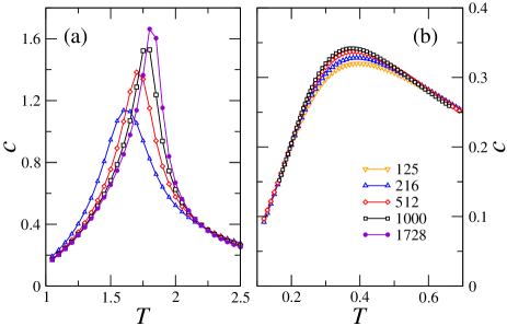
Figure 1: (a) Plots of the specific heat $c$ versus $T$ for volume fraction $\Phi=0.4$. Symbols $\smalltriangledown$, $\smalltriangleup$, $\smalldiamond$, $\smallsquare$, and $\smallblackcircle$ stand for $N=125,216,512,1000$ and $1728$ respectively. (b) Same as in (a) for volume fraction $\Phi=0.1$.

A first overview can be grasped from Figs. 1-2. Fig. 1(a) displays plots of the specific heat $c$ vs $T$ for $\Phi=0.4$. The curves exhibit a marked lambda-shaped peak. Their evident dependence on the number of NP indicates the presence of a singular point in the curve that corresponds to $N\to\infty$ at $T_{c}\approx 1.9$. That singular behavior is expected in PM-FM second order transitions. Data are consistent with a logarithmic divergence of $c$ with $N$. Fig. 1(b) shows the plots obtained for $\Phi=0.1$. In contrast to the previous ones, these plots are smooth and depend little on the sample size. So, there is no sign of any singular behavior. This is expected in PM-SG transitions with strong structural disorder.

FM order entails the presence of non-vanishing magnetization $m$. Fig. 2(a) displays $m_{1}$ vs $T$ for $\Phi=0.4$ at several $N$. They show that $m_{1}$ tends to non-zero values for $N\to\infty$ and low $T$, revealing the existence of strong FM order. The curves plotted in Fig. 2(b) for the magnetic susceptibility $\chi_{m}$ vs $T$ confirm this conclusion as they show peaks that become sharper for large $N$. An extrapolation of the positions of the maxima of those peaks vs $1/N$ provides a value for the transition temperature, $T_{c}(\Phi=0.4)\simeq 1.9(1)$, in agreement with the estimated $T_{c}$ obtained from the analysis of Fig. 1(a). For $T<T_{c}$ we find that $\chi_{m}$ does not diverge with $N$, a fact that validates the above conclusions on FM order. All that is in contrast to the results obtained for $\Phi=0.1$, shown in Fig. 2(c) where we see how the values of $\chi_{m}$ increase with $N$ for low $T$. Data are consistent with a trend $\chi_{m}\sim N^{p}$ for $p\approx 0.45$ and $T\lesssim 0.2$. This behavior suggests the existence of a SG phase.

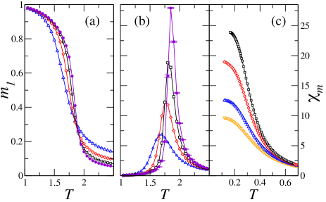
Figure 2: (a) Plots of the magnetization $m_{1}$ versus $T$ for volume fraction $\Phi=0.4$. Symbols $\smalltriangledown$, $\smalltriangleup$, $\smalldiamond$, $\smallsquare$, and $\smallblackcircle$ stand for $N=125,216,512,1000$ and $1728$ respectively. b) Plots of the magnetic susceptibility $\chi_{m}$ versus $T$ for volume fraction $\Phi=0.4$. Same symbols as in (a). (c) Same as in (b) but for volume fraction $\Phi=0.1$.

Let us discuss now the threshold value of $\Phi$ at which the FM order disappears. Mean-field calculations predict that FM order persists for $\Phi\geq\Phi_{c}=\pi/20\sim 0.157$.zhang

The plots in Fig. 3 show that the FM order persists at $\Phi=0.18$. The curves of $m_{1}$ vs $T$ in panel (a) indicate an increase in magnetization with $N$ at low $T$, although they also exhibit relevant finite size effects. The Binder parameter of panel (b) allows to determine the transition temperature within good precision. In general this parameter tends to 1 for $N\rightarrow\infty$ in FM phases, while from the law of large numbers it follows that in PM phases $B_{m}\rightarrow 0$ as $N$ increases. On the other hand, since $B_{m}$ is dimensionless, it must be independent of $N$ at the critical point. As a consequence, curves of $B_{m}$ vs $T$ for different values of $N$ cross at $T_{c}$ for second order transitions. Instead, in presence of an intermediate marginal phase of quasi-long-range FM order, the curves do not cross but join. Plots of $B_{m}$ vs $T$ for several $N$ are shown in Fig. 3(b) for $\Phi=0.18$. Those curves cross at a well defined critical temperature for $N\geq 512$. extra With similar results obtained for $\Phi\geq 0.17$, we can draw a line of transition between PM and FM phases.

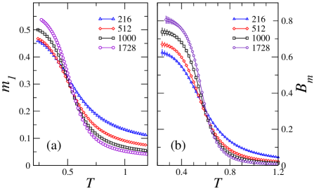
Figure 3: (a) Plots of the magnetization $m_{1}$ vs $T$ for $\Phi=0.18$. Symbols $\smalltriangleup$, $\smalldiamond$, $\smallsquare$, and $\smallcircle$ stand for $N=216,512,1000$ and $1728$ respectively. (b) Plots of the Binder cumulant of the magnetization $B_{m}$ vs $T$ for $\Phi=0.18$. Same symbols as in (a).

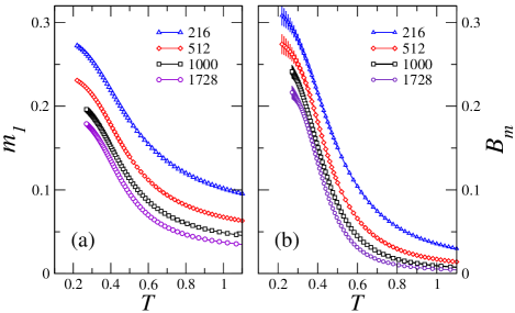
Figure 4: (a) Plots of the magnetization $m_{1}$ vs $T$ for $\Phi=0.14$. Symbols $\smalltriangleup$, $\smalldiamond$, $\smallsquare$, and $\smallcircle$ stand for $N=216,512,1000$ and $1728$ respectively. (b) Plots of the Binder cumulant of the magnetization $B_{m}$ vs $T$ for $\Phi=0.18$. Same symbols as in (a).

The corresponding plots for $\Phi=0.14$ are shown in Fig. 4. The qualitatively different results illustrate the absence of FM order at this value of $\Phi$. The plots of the magnetization in panel (a) show that $m_{1}$ gradually decreases as $N$ increases for all $T$. The data of $m_{1}$ for low temperature agree with an algebraic decay $m_{1}\sim N^{p}$ for $p<1/2$, hence a marginal order is a priori not excluded. However, the plots of $B_{m}$ vs $T$ from panel (b) show clearly that $B_{m}$ vanishes for $N\to\infty$ for all $T$, and this means that the FM order is short ranged even at low temperature. We have obtained similar plots for all analysed values of $\Phi$ in the range $\Phi\leq 0.15$, and this fact excludes FM order.

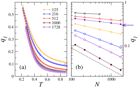
Figure 5: (a) Plots of the SG overlap parameter $q_{1}$ vs $T$ for $\Phi=0.14$. Symbols $\smalltriangledown$, $\smalltriangleup$, $\smalldiamond$, $\square$ and $\smallcircle$ stand for $N=125,216,512,1000$ and $1728$ respectively. (b) Log-log plots of $q_{1}$ vs $N$ for several temperatures at $\Phi=0.14$. From top to bottom, $\smalltriangledown$, $\smalltriangleup$, $\smallblackdiamond$, $\smalldiamond$, $\square$ and $\smallcircle$ and $\smallblackcircle$ stand for $T=0.22,~{}0.27,~{}0.31~{}0.37,~{}0.47,~{}0.57$ and $0.96$ respectively. The arrow marks the data set corresponding to the SG-PM transition temperature. The dashed line shows the $N^{-1/2}$ decay expected for a paramagnet.

It is then imperative to investigate whether at those values of $\Phi$ the FM phase is replaced by SG order. For this purpose we have evaluated the overlap parameter $q_{1}$ in Fig. 5. In panel (a) we show plots of $q_{1}$ vs $T$ for $\Phi=0.14$. It is instructive to compare these plots with those for $m_{1}$ in Fig. 4(a) for the same value of $\Phi$. We notice that like for $m_{1}$, also the overlap $q_{1}$ decreases when $N$ increases for all temperatures. To determine if $q_{1}$ tends to zero in the limit $N\rightarrow\infty$, we have prepared log-log plots of $q_{1}$ vs $N$ in Fig. 5(b). Data in these plots are consistent with a behavior $q_{1}\sim 1/N^{p}$ at low temperatures where $p$ is a $T$-dependent exponent. Thus, for example, at $T=0.31$ we have obtained $p\simeq 0.11$. The expected behavior for a PM phase is $N^{-1/2}$, but we have found it only at high temperature. These properties can be due to the presence of SG with quasi-long-range order at low $T$. To verify it we have examined the behaviors of $B_{q}$ and $\xi_{L}/L$ in terms of $T$. Recall indeed that in the thermodynamic limit $B_{q}\to 1$ when there is strong SG order, becomes zero in the PM phase, and tends to an intermediate value at critical points. A similar trend is expected for dimensionless magnitudes like $\xi_{L}/L$ with a caveat: in case of strong order, this quantity diverges as $N^{1/2}$ instead of going to $1$. This makes the splay out of curves for $\xi_{L}/L$ for different sizes at low temperatures more prominent than for $B_{q}$, and the crossing points are clearer for second order transitions.longi

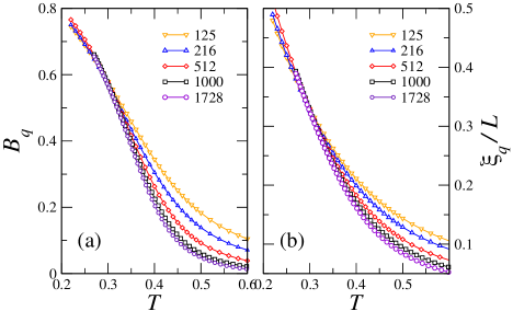
Figure 6: (a) Plots of the SG correlation length $\xi_{L}/L$ vs $T$ for $\Phi=0.14$. Symbols $\smalltriangledown$, $\smalltriangleup$, $\smalldiamond$, $\square$ and $\smallcircle$ stand for $N=125,216,512,1000$ and $1728$ respectively. (b) Plots of the SG correlation lenght $\Xi_{L}/L$ vs $T$ for $\Phi=0.14$. Same symbols as in (a).

The curves $B_{q}$ vs $T$ for $\Phi=0.14$ shown in Fig. 6(a) merge at $T$ below a certain value $T_{sg}\simeq 0.31(2)$, rather than crossing. The spread that those curves exhibit for $T<T_{sg}$ becomes almost zero for $N\geq 512$. Thus, $B_{q}$ does not tend to 1 in the thermodynamic limit. Then, the curves $B_{q}$ collapse for $N\to\infty$ and $T\leq T_{sg}$, and this is consistent with the algebraic decay found for $q_{1}$. The plots of $\xi_{L}/L$ vs $T$ in Fig. 6(b) exhibit a similar behavior. All that emphasizes that there exists SG order with quasi-long-range order, as it happens in other systems with NP and strong structural disorder.

The temperature $T_{sg}$ that marks the transition between PM and SG orders is a function of $\Phi$ and for that reason it will be represented as $T_{sg}(\Phi)$. The fact that the merging of different curves be dominant over crossing makes the determination of $T_{sg}(\Phi)$ less precise than for the PM-FM transition. In any case $T_{sg}(\Phi)$ is quite smooth as a function of $\Phi$ for strong dilution. For $\Phi=0.1$ we have obtained $T_{sg}/\Phi=1.9(1)$, in agreement with the relation $T_{sg}=x$ found in the limit of strong dilution for systems of dipoles in crystalline simple cubic (SC) lattices with fraction $x$ of occupied sites.PADdilu For a diluted system of spheres with SC order, this relation reads $T_{sg}/\Phi=1/\Phi_{SC}\simeq 1.91$, where $\Phi_{SC}$ is the volume fraction for SC lattices.

As a last step we determine the low temperature boundary of the FM phase. Mean-field theory predicts the onset of FM order for $T=0$ at $\Phi_{c}=0.157$. Let us examine first the data obtained for $\Phi=0.16$. Plots of $B_{q}$ vs $T$ for various sizes are shown in Fig. 7(b). We estimate that the curves cross at $T_{c}\approx 0.44$. For $T<T_{c}$ we have found (not shown) that $q$ does not vanish in the thermodynamic limit, a fact that points to the presence of SG order. Contrarily, the curves of $B_{m}$ vs $T$ shown in panel (a) of the same figure merge at low temperatures. In particular, the curves for $N=1000$ and $N=1177$ fall on top of each other within the error bars for $T<T_{c}$. This suggests that the transition line between FM and SG lies at $\Phi\approx 0.16$ at low temperature.

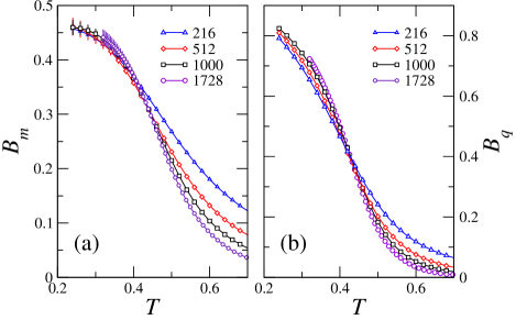
Figure 7: (Color online) (a) Plots of the Binder cumulant $B_{m}$ vs $T$ for $\Phi=0.16$. $\smalltriangleup$, $\smalldiamond$, $\square$ and $\smallcircle$ stand for systems with $N=216,512,1000$ and $1728$ dipoles respectively. (b) Plots of the Binder cumulant for the overlap parameter $B_{q}$ vs $T$ for $\Phi=0.16$. Same symbols as in (a).

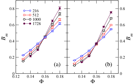
Figure 8: (a) Plots of the Binder cumulant $B_{m}$ vs $\Phi$ for $T=0.28$. $\smalldiamond$, $\smallsquare$ and $\smallcircle$ and $\smallblackcircle$ stand for systems with $N=216,512,1000$ and $1728$ dipoles respectively. (b)The same as in (a) but for temperature $T=0.40$.

This line of critical points can be recovered in a more precise way with data obtained from simulations in the range $0.13<\Phi<0.18$. To this end, we prepare plots of $B_{m}$ vs $\Phi$ at different $N$ along isotherms for $T$ below the PM region. Fig. 8 shows the plots for the isotherm at $T=0.28$ in panel (a) and $T=0.4$ in panel (b). Recall that $B_{m}$ diminishes as $N$ increases in the SG phase while in the FM phase $B_{m}$ increases with $N$. As shown by both panels in the figure, we have found that the curves of $B_{m}$ vs $\Phi$ cross at the transition $\Phi_{c}(T)$. A very precise result can be obtained if we have many values of $\Phi$ available. The transition line $\Phi_{c}(T)$ is almost vertical at $\Phi=0.160(5)$ in good agreement with mean-field approximation. We also notice the well defined separation in the curves above and below the cross point in the plots of Fig. 8. This detail rules out the possibility of the presence of critical phases in between FM and SG in the region close to $\Phi\simeq\Phi_{c}(T)$.

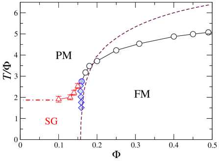
Figure 9: Phase diagram in the plane $(T,\Phi)$ for the fully textured dipolar Ising model on random HS-like configurations. Symbols $\medcircle$ stand for PM-FM transition obtained from the $B_{m}$ vs $T$ plots. Symbols $\triangle$ stand for PM-SG transition obtained from the $B_{q}$ vs $T$ plots. Symbols $\meddiamond$ represent the FM-SG transition and follow from the $B_{m}$ vs $\Phi$ plots. Error bars are smaller than the size of these symbols. The dashed line stand for a mean-field calculation by Zhang-Widom.zhang The horizontal red dashed line comes from previous calculations for strongly diluted DIS in crystals.

The results of this section can be gathered in the phase diagram of Fig. 9 which shows the extension of the several FM, SG and PM regions. They are separated by second order transition lines. The slope of the transition line at low density is fairly zero, in such a way that the ratio $T_{sg}/\Phi$ takes a fixed value, $T_{sg}/\Phi\simeq 1.9$. Mean-field theory yields a good approximation of the boundary line of the FM phase at low temperatures.zhang This approximation is carried out by assuming fully random particle positions which is in contrast with the results obtained for systems of dipoles with no local anisotropy,alonso20 for which the onset found at $\Phi=0.49$ coincides with the freezing point of the hard sphere fluid. This onset depends on the details of the radial distribution function for short distances.doublehorn We end this discussion by noticing that differently from systems of Ising dipoles with orientational disorder,alonso19 we have found for the systems studied in this paper no trace of reentrances or other intermediate phases, as clearly shown in Fig. 9.

III.2 FM order on anisotropic DHS fluid-like configurations

In this subsection we will describe the results obtained by exploring the FM order of textured Ising dipoles placed in frozen DHS fluid-like distributions of particles. These positional distributions are taken from equilibrium configurations of the DHS fluid at low temperatures $T_{f}$.malherbe23 We consider volume fractions in the range $0.25\lesssim\Phi\lesssim 0.5$ for which the DHS fluid is known to polarize below the transition temperature, $T_{c}(DHS,\Phi)$.weis ; weis2 Within this interval of values of $\Phi$ and for a wide range of temperatures $T_{f}$ below $T_{c}(DHS,\Phi)$ the equilibrium configurations for the DHS fluid exhibit some partial alignment of the magnetic moments ${\widehat{\mu}_{i}}$ along a common direction and a certain degree of anisotropy in the positional distribution. At the same time these fluid-like configurations are still homogeneus and show absence of crystalline order.weis2 It is this type of configurations that arise naturally in colloidal suspensions of particles at low temperature.

Any of those equilibrium configurations is determined by the positions $\vec{r}_{i}$ and the instantaneous orientations of the magnetic moments $\widehat{\mu}_{i}$ of all particles, $i=1,\dots,N$. At low $T_{f}$ the orientations exhibit nematic order along a preferred direction $\widehat{a}$. In this case the configurations are said to be partially textured.

As it is customary when studying nematic order, the direction $\widehat{a}$ can be determined as the eigenvector related to the largest eigenvalue of the so-called nematic tensor allen

$$\bar{Q}_{n}=\frac{1}{2N}\sum_{i}(3{\widehat{\mu}_{i}}{\widehat{\mu}_{i}}-\bar{I})\;.$$ (13)

Thus, the degree of texturation can be quantified by the value of the nematic order parameter $\lambda_{n}$. Similarly, the degree of anisotropy in the disordered positional distribution can be assessed by the structural nematic order parameter $\lambda_{s}$ associated with the tensor

$$\bar{Q}_{s}=\frac{1}{2N_{nn}}\sum_{nn}(3{\widehat{r}_{nn}}{\widehat{r}_{nn}}-\bar{I})\;,\$$ (14)

where $\widehat{r}_{nn}$ are the normalized relative positions $\widehat{r}_{ij}\equiv\vec{r}_{ij}/{r}_{ij}$ between pairs of particles whose $r_{ij}$ distance is smaller than a threshold value chosen as $r_{s}=1.2d$, and $N_{nn}$ is the number of such pairs. holdsworth $\lambda_{s}$ is the largest eigenvalue of $\bar{Q}_{s}$ and measures the degree of aligment of the set of $\widehat{r}_{nn}$ along a preferred direction.

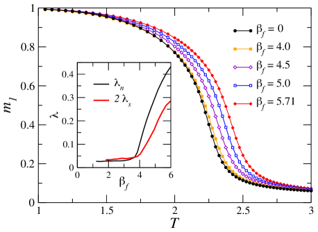
Figure 10: Plots of the magnetization $m_{1}$ vs $T$ for ensembles of $N=1177$ dipoles placed on anisotropic frozen configurations obtained for $\Phi=0.45$ and the inverse freezing temperatures $\beta_{f}$ indicated in the figure. The inset shows the structural $\lambda_{s}$ and the orientational $\lambda_{n}$ nematic order parameter for the DHS fluid versus the inverse temperature $\beta_{f}$ for density $\Phi=0.45$ and $N=1177$ (data taken from Ref. malherbe23, ).

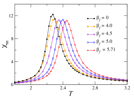
Figure 11: Plots of the susceptibility $\chi_{m}$ vs $T$ for ensembles of $N=1177$ dipoles placed on anisotropic frozen configurations obtained for $\Phi=0.45$ and the inverse freezing temperatures $\beta_{f}$ indicated in the figure.

The behavior of those eigenvalues has been explored for $\Phi=0.45$ and $\Phi=0.262$ in Ref. malherbe23, . Plots of $\lambda_{n}$ and $\lambda_{s}$ versus the inverse temperature $\beta_{f}=1/T_{f}$ are given for $\Phi=0.45$ and $N=1177$ in the inset of Fig. 10. The plateaux found for $\beta_{f}\lesssim\beta_{c}(DHS,\Phi)=4$ with $\lambda_{s}\simeq\lambda_{n}\simeq 0$ indicate that the configurations remain isotropic for temperatures above the PM-FM transition, (the notation $\beta_{c}(DHS,\Phi)\equiv 1/T_{c}(DHS,\Phi)$ has been used). In contrast, for $\beta_{f}\gtrsim 4$ both $\lambda_{n}$ and $\lambda_{s}$ increase with $\beta_{f}$, indicating that the double anisotropy strengthens as temperature is lowered. For $\Phi=0.262$, where $\beta_{c}(DHS,\Phi)=7.7$, the behavior is qualitatively the same, apart from the fact that there seems to form chains of spheres at very low temperature instead of the homogeneous configurations observed for $\Phi=0.45$.

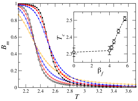
Figure 12: (a) Plots of $B_{m}$ vs $T$ for systems of $N$ dipoles placed on anisotropic frozen configurations obtained for $\Phi=0.45$ and given freezing temperatures $\beta_{f}$. $\smallblacktriangleup$, $\smallblackdiamond$ and $\smallblacksquare$ stand for $\beta_{f}=5.71$ and system sizes $N=453,758$ and $1177$ respectively. $\smallcircle$, $\smalltriangleup$, $\smalldiamond$ and $\smallsquare$ stand for $\beta_{f}=0$ and $N=125,216,512$ and $1000$ respectively. The solid lines are guides to the eye. The inset shows the PM-FM transition temperature $T_{c}$ vs $\beta_{f}$ for volume fraction $\Phi=0.45$.

Up to here, we have described equilibrium DHS fluid-like configurations at low $T$ which exhibit partial texturation in the orientations of the dipoles as well as structural anisotropy in their positions.malherbe23 However, given that this work is aimed at the study of the role of frozen positional disorder, we proceed by studying fully textured systems of DHS fluid-like configurations in equilibrium. Once picked one of these configurations, i.e., once the sets of positions $\vec{r}_{i}$ and momenta $\widehat{\mu}_{i}$ are fixed throughout the lattice, the frozen textured distribution is built by firstly computing the nematic tensor $\bar{Q}_{n}$ and secondly by choosing the nematic director $\widehat{a}$ of $\bar{Q}_{n}$ as the common direction along which all the Ising dipoles are placed.

The question now is how the remaining structural positional anisotropy in those systems affects the order at low $T$. We do not expect to find any SG order for the volume fractions considered here ($0.25\lesssim\Phi\lesssim 0.5$). Note from the previous section, that for $\Phi\lesssim 0.16$ only FM order is expected at low $T$ even for isotropic configurations. Thus, by studying DHS systems we intend to analyze whether the structural positional anisotropy enhances the FM order already present in isotropic HS configurations.

Curves of magnetization $m_{1}$ vs $T$ are shown in Fig. 10 for $\Phi=0.45$ and $N=1177$ at various values of $\beta_{f}=1/T_{f}$. The system at low temperature is in a FM phase even for $\beta_{f}=0$ in absence of anisotropy, in agreement with the previous subsection. The result for $\beta_{f}\simeq\beta_{c}(DHS,\Phi)\simeq 4$ is practically the same that for $\beta_{f}=0$. Only for $\beta_{f}>4$ we see the curves of magnetization to move rightwards as $\beta_{f}$ increases, a fact that indicates that the increase in anisotropy favors FM order. The susceptibility $\chi_{m}$ vs $T$ curves shown in Fig. 11 exhibit peaks which are typical for ferromagnets. The positions of those peaks for $\beta_{f}>4$ shift to the right as $\beta_{f}$ is increased, indicating that the PM-FM transition temperature $T_{c}$ increases with the anisotropy.

A precise determination of $T_{c}$ can be obtained from the crossing points of the Binder parameter vs $T$ for different sizes, as shown in Fig. 12. The inset in this figure shows the transition temperature $T_{c}$ vs $\beta_{f}$ for $\Phi=0.45$. This figure is to be compared with the inset of Fig. 10. We can appreciate that $T_{c}$ increases with $\beta_{f}$ only for $\beta_{f}>\beta_{c}(DHS,\Phi)\simeq 4$ when the structural anisotropy quantified by $\lambda_{s}$ increases. It is worth to mention that for $\beta_{f}\gtrsim 4$ the values of $T_{c}$ obtained here for fully textured systems along the nematic director $\widehat{a}$ practically coincide with the values of $T_{c}$ found for ensembles of Ising dipoles placed on the same frozen configurations $\{\vec{r}_{i}\}$ but pointing up or down along the orientations $\{\widehat{\mu}_{i}\}$ of the original DHS configurations. malherbe23 This suggests that the procedure used in this work for imposing a common direction $\widehat{a}$ (obtained from the set of values $\widehat{\mu}_{i}$) to build fully textured samples keeps all the relevant information for the FM order induced by the structural anisotropy on positions. In other words, the fluctuations of the Ising axes around the mean value $\widehat{a}$ play only a marginal role.

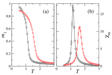
Figure 13: (a) Plots of the magnetization $m_{1}$ vs $T$ for ensembles of $N=1000$ dipoles placed on anisotropic frozen configurations obtained for $\Phi=0.262$. Symbols $\smallcircle$ and $\smalldiamond$ stand for $\beta_{f}=0$ and $8.5$ respectively. (b) Plots of the susceptibility $\chi_{m}$ vs $T$ for ensembles of $N=1000$, for $\Phi=0.262$. Same symbols as in (a).

For the volume fraction $\Phi=0.262$ similar results are obtained. Fig. 13 exhibits curves of $m_{1}$ and $\chi_{m}$ vs $T$ for $\beta_{f}=0$ and $\beta_{f}=8.5$ (a value larger than $\beta_{c}(DHS,\Phi)=7.7$). Both $m_{1}$ and $\chi_{m}$ curves move to the right as $\beta_{f}$ is increased, indicating again that the presence of structural anisotropy favors FM order. However it can be noticed that for very low temperatures the magnetization $m_{1}$ for $\beta_{f}=8.5$ is lower than for $\beta_{f}=0$. This fact can be related to the formation of inhomogenities in the DHS fluid for low $T_{f}$.weis2 ; malherbe23

IV CONCLUSIONS

We have studied by Monte Carlo simulations the effect of positional disorder on the collective properties of fully textured systems of identical magnetic nanospheres that behave as Ising dipoles along common easy axes.

We have first studied frozen isotropic systems of hard spheres obtained along the stable liquid branch with volume fraction $\Phi$ ranging from low values up to the freezing point ($\Phi\simeq 0.49$). By analysing the phase diagram on the $T$-$\Phi$ plane, we have found a low-temperature ferromagnetic phase for $\Phi\gtrsim\Phi_{o}=0.160(5)$ in good agreement with mean-field calculations that assume complete randomness in positions. This phase exhibits strong long-range order. For $\Phi\less\Phi_{o}$ this ferromagnetic phase disappears giving rise to a spin-glass phase for temperatures below $T_{sg}(\Phi)$. For strong dilution we find $T_{sg}(\Phi)/\Phi=1.9(1)$. The nature of the dipolar spin-glass phase is similar to the one observed in other systems of Ising dipoles with strong frozen disorder. Plots of Binder cumulants vs $\Phi$ allow to obtain the transition line between the ferromagnetic and spin-glass phases. We find neither an appreciable reentrance nor an intermediate region with quasi-long-range ferromagnetic between the FM and SG phases.

We have also studied anisotropic spatial systems for $\Phi=0.45$ and $\Phi=0.262$. They have been obtained by freezing the liquid state of the dipolar hard sphere fluid in its polarized state at sufficiently low temperatures $T_{f}$. Such systems develop some texturation as well as anisotropic spatial correlations that increase as $T_{f}$ is decreased. The ferromagnetic order of parallel dipoles placed on such configurations along their nematic director is enhanced as $T_{f}$ decreases.

References

- (1) R. P. Cowburn, Philos. Trans. R. Soc. London, Ser. A 358, 281 (2000); R. J. Hicken, ibid. 361, 2827 (2003).
- (2) R. Skomski, J. Phys.: Condens. Matter, 2003, 15, R841 (2003).
- (3) S. Bedanta, and W. Kleeman J. Phys. D: Appl. Phys. 42 013001 (2009); S. A. Majetich and M. Sachan, J. Phys. D: Appl. Phys. 39, R407 (2006).
- (4) D. Fiorani, and D. Peddis J. Phys. Conf. Ser., 521, 012006 (2014).
- (5) E. H. Sánchez, M. Vasilakaki, S. S. Lee, P. S. Normile, M. S. Andersson, R. Mathieu, A. López-Ortega, B. P. Pichon, D. Peddis, C. Binns, P. Nordblad, K. Trohidou, J. Nogués, J. A. de Toro, Small 18, 2106762 (2022).
- (6) J. A. de Toro, S. S. Lee, D. Salazar, J. L. Cheong, P. S. Normile, P. Muñiz, J. M. Riveiro, M. Hillenkamp, F. Tournus, A. Amion, and P. Nordblad, Appl. Phys. Lett. 102, 183104 (2013); M. S. Andersson, R. Mathieu, S. S. Lee, P. S. Normile, G. Singh, P. Nordblad, and J. A. de Toro, Nanotechnology 26, 475703 (2015); M. S. Andersson, J. A. De Toro, S. S. Lee, P. S. Normile, P. Nordblad, and R. Mathieu, Phys. Rev. B 93, 054407 (2016).
- (7) S. Nakamae, J. Magn. Magn. Mater. 355, 225 (2014).
- (8) J. Luttinger, and L. Tisza, Phys. Rev. B, 72, 257 (1942); J. F. Fernández and J.J. Alonso, Phys. Rev. B, 62, 53 (2000); J. Batle, and O. Ciftja, Sci. Rep. 10, 19113 (2020).
- (9) S. J. Knak Jensen, and K. Kjaer, J. Phys.: Condens. Matter 1, 2361 (1989).
- (10) D. Peddis, S. Laureti, and D. Fiorani, New Trends in Nanoparticle Magnetism (Springer Series in Materials Science Series, Vol. 308 , 2021).
- (11) X. Batlle, C. Moya, M. Escoda-Torroella, O. Iglesias, A. Fraile Rodriguez, and A. Labarta J. Magn. Magn. Mater. 543, 168594 (2022).
- (12) J. Dobson Nature Mater. 11 1106 (2012).
- (13) Q. A. Panhurst, N. T. K. Thanh, S. K. Jones, and J. Dobson, J. Phys. D: Appl. Phys. 42 224001 (2009); X. Li, J. Wei, K.E. Aifantis, Y. Fan, Q. Feng, F.-Z. Cui, F. Watari, J. Biomed. Mater. Res. 104 1285 (2016).
- (14) S. Nakamae, C. Crauste-Thibierge, D. L’Hôte, E. Vincent, E. Dubois, V. Dupuis, and R. Perzynski, Appl. Phys. Lett. 101, 242409 (2010).
- (15) S. Sahoo, O. Petracic, W. Kleemann, P. Nordblad, S. Cardoso, and P. P. Freitas, Phys. Rev. B 67, 214422 (2003).
- (16) S. Mørup, Europhys. Lett. 28, 671 (1994).
- (17) V. Russier, and J. J. Alonso, J. Phys.: Condens. Matter, 32, 135804 (2020).
- (18) J. J. Alonso, B. Allés, and V. Russier, Phys. Rev. B, 100, 134409 (2019).
- (19) V. Russier, J. J. Alonso, I. Lisiecki, A. T. Ngo, C. Salzemann, S. Nakamae, and C. Raepsaet, Phys. Rev. B, 102, 174410 (2020).
- (20) J. J. Alonso, B. Allés, and V. Russier, Phys. Rev. B, 102, 184423 (2020).
- (21) H. Zhang, and M. Widom, Phys. Rev. B 51, 8951 (1995).
- (22) C. Moya, O. Iglesias, X. Batlle, and A. Labarta. J. Phys. Chem. C, 119 24142 (2015).
- (23) J. J. Weis, and D. Levesque, Phys. Rev. E 48, 3728 (1993)
- (24) J. J. Weis, J. Chem. Phys., 123, 044503 (2005); C. Holm, and J. J. Weis, Curr. Opin. Colloid Interface Sci., 10, 133 (2005).
- (25) J. G. Malherbe, V. Russier, and J. J. Alonso J. Phys.: Condens. Matter, 35, 305802 (2023).
- (26) G. Ayton, M. J. P. Gingras, and G. N. Patey, Phys. Rev. Lett. 75, 2360 (1995); G. Ayton, M. J. P. Gingras, and G. N. Patey, Phys. Rev. E 56, 562 (1997).
- (27) K. M. Tam, and M. J. P. Gingras Phys. Rev. Lett. 103, 087202 (2009); J. J. Alonso and J. F. Fernández, Phys. Rev. B 81, 064408 (2010);
- (28) B. D. Lubachevsky, and F. H. Stillinger, J. Stat. Phys. 60, 561 (1990).
- (29) S. Torquato, and F. H. Stillinger, Rev. Mod. Phys. 82, 2633 (2010).
- (30) M. Skoge, A. Donev, F.H. Stillinger, and S. Torquato, Phys. Rev. E 74, 041127 (2006).
- (31) E. Marinari and G. Parisi, Europhys. Lett. 19, 451 (1992); K. Hukushima and K. Nemoto, J. Phys. Soc. Jpn. 65, 1604 (1996).
- (32) N. A. Metropolis, A. W. Rosenbluth, M. N. Rosenbluth, A. H. Teller, and E. Teller, J. Chem. Phys 21, 1087 (1953).
- (33) I. Rozada, M. Aramon, J. Machta, and H.G. Katzgraber, Phys. Rev. E 100, 043311 (2019).
- (34) J. J. Alonso, and B. Allés, J. Phys.: Condens. Matter, 29, 355802 (2017).
- (35) P. Ewald, Ann. Phys. (Leipzig) 64, 253, (1921).
- (36) Z. Wang, and C. Holm, J. of Chem. Phys. 115, 6351 (2001).
- (37) M. P. Allen, and D. J. Tildesley, Computer simulation of Liquids, 1st ed. (Clarendon, Oxford, 1987).
- (38) S. F. Edwards and P. W. Anderson, J. Phys. F, 5, 965 (1975).
- (39) For some values of , pairs of curves do not cross precisely at the same point, but extrapolations of the crossing points allow to obtain well defined values of .
- (40) M. Palassini, and S. Caracciolo, Phys. Rev. Lett., 82, 5128 (1999).
- (41) For volume fractions below the HS fluid is in a stable liquid phase. Compressing rapidly this fluid results in the appearance of metastable branches of amorphous states with densities up to . For this glassy states with , the radial distribution function exhibits characteristic double-horn peaks at and where is the diameter or size of the NP. In absence of local anisotropies, Monte Carlo simulations find that the existence of FM for systems of dipoles in RDP depends on the presence of this double-horn.
- (42) M. J. P. Gingras, and P.C.W. Holdsworth, Phys. Rev. Lett., 74, 202 (1995).