Data-driven discovery of relevant information in quantum simulators

Abstract

Quantum simulators offer powerful means to investigate strongly correlated quantum matter. However, interpreting measurement outcomes in such systems poses significant challenges. Here, we present a theoretical framework for information extraction in synthetic quantum matter, illustrated for the case of a quantum quench in a spinor Bose-Einstein condensate experiment. Employing non-parametric unsupervised learning tools that provide different measures of information content, we demonstrate a theory-agnostic approach to identify dominant degrees of freedom. This enables us to rank operators according to their relevance, akin to effective field theory. To characterize the corresponding effective description, we then explore the intrinsic dimension of data sets as a measure of the complexity of the dynamics. This reveals a simplification of the data structure, which correlates with the emergence of time-dependent universal behavior in the studied system. Our assumption-free approach can be immediately applied in a variety of experimental platforms.

I Introduction

Recent remarkable advances in highly controlled synthetic quantum devices have revolutionized the study of strongly correlated systems Bloch et al. (2008); Lewenstein et al. (2012); Georgescu et al. (2014); Gross and Bloch (2017); Daley et al. (2022); Cao et al. (2019). A key element of many of such platforms is their capacity to produce large data sets of many-body snapshots, for example, via generalized projective measurements of the entire wave function Kunkel et al. (2019). However, the analysis of such outcome poses in general serious challenges, which typically force us to rely on assumptions for certain quantities, disregarding part of the information content of the generated data—in data science language, a dimensional reduction with an uncontrolled loss of information. A particularly important problem is the identification of the most informative observables to describe such quantum many-body systems—a paramount task at the core of quantum field theory Tsvelik (2003); Kleinert (2018), that is even more daunting for systems driven out of equilibrium. To address this, one needs to develop methods to process the maximum amount of information in quantum simulator output, which are able to identify relevant features—and thus degrees of freedom—emerging from the underlying physical system, without making any assumption nor uncontrolled dimensional reduction.

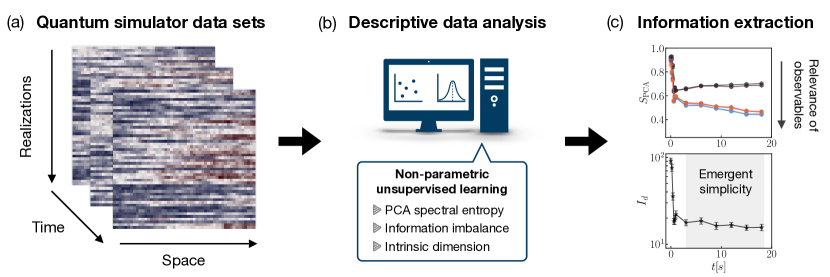
Figure 1: Assumption-free unveiling of relevant information in quantum simulation. (a) We start from snapshots of a many-body system, which are represented as 2D arrays at different times. At a fixed time, each row corresponds to a different realization, while each column is a different data feature, e.g., the atomic density in a given magnetic substate at a given spatial location. (b) Using non-parametric unsupervised learning tools, we perform an exploratory analysis to uncover interesting features of the data, without making any assumptions. (c) From this description, we infer relevant properties of the physical system: (Upper panel) By quantifying the information content and correlations in a data set, the principal component analysis entropy provides a measure of relevance of observables, thence guiding the identification of the most informative degrees of freedom. (Lower panel) After a quick fall to relatively small values, the intrinsic dimension of data sets features a long, stable plateau as a function of time (shaded region), providing a lower bound for the timescale after which the dynamics may become simpler and be captured by universal scaling.

In this work, we introduce a theoretical framework for data-driven information discovery in quantum simulation, which is schematically illustrated in Fig. 1. We start by considering collections of independent quantum simulator snapshots, which resolve, for example, the dynamics of a many-body system in space and time [Fig. 1(a)]. Such data sets are characterized using non-parametric unsupervised learning methods [Fig. 1(b)]. Finally, from this system-agnostic and unsupervised description of the data, we infer relevant information for the physical system under study [Fig. 1(c)].

This framework is based on three techniques: (i) spectral entropies calculated from a principal component analysis (PCA) of the data, (ii) the information imbalance between a subset and the full set of observations, and (iii) the intrinsic dimension of the concomitant data manifolds. These tools which quantify—from different angles—the information content and correlations in the data, have found several successful applications in various fields, such as chemical and biomolecular science Alter et al. (2000); Varshavsky et al. (2006, 2007); Glielmo et al. (2022); Donkor et al. ; Facco et al. (2017, 2019); Allegra et al. (2020); Glielmo et al. (2021), ecology Strydom et al. (2021), stock market dynamics Caraiani (2014); Gu et al. (2015); Gu and Shao (2016); Chakraborti et al. (2020); Alvarez-Ramirez and Rodriguez (2021); Espinosa-Paredes et al. (2022), and image analysis Levina and Bickel (2004); Gong et al. (2019); Pope et al. (2021); Weng et al. (2022).

To demonstrate the capabilities of our approach we apply it to experimental data of a spinor Bose-Einstein condensate (BEC) Prüfer et al. (2020): we evaluate the full set of experimentally measured densities without knowledge of the post-processing steps which are necessary in order to infer the relevant spin variables from them. Our main results are as follows: (I) PCA spectral entropies and information imbalance allow for a theory-agnostic determination of the most informative measured observables. The predictive power of these methods is demonstrated by showing that they can also unveil combinations of the measured densities, which are key to describe the spin structure of the system Prüfer et al. (2018, 2020); Stamper-Kurn and Ueda (2013); Kawaguchi and Ueda (2012). (II) The behavior of the intrinsic dimension as a function of time, displays a rapid decay to significantly smaller values, after which it features very long, stable plateaus. As argued below, this observation is in strong agreement with the formation of spin structure and the emergence of self-similar dynamics Berges et al. (2015); Prüfer et al. (2018); Erne et al. (2018); Prüfer et al. (2020); Glidden et al. (2021).

The remaining of this paper is structed as follows: In Sec. II, we introduce the different data science methods used in this work. We describe the spinor BEC experiment and the structure of our data sets in Sec. III. In Sec. IV, we present a theory-agnostic scheme to identify relevant fields, in a systematic and unbiased way, directly from (a limited number of) experimental observations. In Sec. V, we complement our data-driven analysis by characterizing the Kolmogorov complexity of the studied quantum dynamics, and address its capability of recognizing physical information. Conclusions and possible extensions of our work are discussed in Sec. VI.

II Methods

Before diving into the central part of our paper, we present an introduction to the data science tools that are employed in this work. We focus on non-parametric methods that are oriented towards extracting information from data, without making (strong) assumptions on the functional form of the probability distribution underlying the data. For the purpose of this exposition, we consider here an abstract data set, structured as a rectangular matrix ${\bf X}=\{\vec{X}^{i}\}_{i=1}^{N_{r}}$, of dimension $N_{r}\times p$, where each $p$-dimensional row vector $\vec{X}^{i}$ represents a single realization (observation) of a set of $p$ features (input variables) that are measured in all realizations. This type of structure is ubiquitous to both stochastic Monte Carlo simulations, as well as quantum experiments featuring projective measurements of a large number of degrees of freedom. In the next section, we shall define precisely the concrete data sets that will be analysed with the techniques presented below.

II.1 Principal component analysis entropy

Principal component analysis is one of the most popular non-parametric methods for unsupervised learning, and has found a vast number of applications, including classical and quantum many-body problems Wang (2016); Hu et al. (2017); Costa et al. (2017); Wetzel (2017); Wang and Zhai (2017); Ch’ng et al. (2018); Khatami (2019); Turkeshi (2022). The central idea of PCA is to use an orthogonal transformation to seek for directions along which the data exhibit most variation Jolliffe (2005); Mehta et al. (2019). This is motivated by empirical evidence showing that in many cases such “high-variance” directions capture the relevant information of the data. This problem reduces to diagonalizing the sample covariance matrix ${\bf\Sigma}={{\bf X}^{\star}}^{T}{\bf X}^{\star}/(N_{r}-1)$, where ${\bf X}^{\star}$ is the column-centred data matrix in which the mean value of each column is subtracted from the entries in the column. The solution to the eigenvalue-eigenvector problem ${\bf\Sigma}\vec{w}_{k}=\lambda_{k}\vec{w}_{k}$, yields $\lambda_{1}\geq\lambda_{2}\geq\cdots\geq\lambda_{R}\geq 0$ ($R\leq\mathrm{min}\{N_{r},p\}$ is the rank of ${\bf X}^{\star}$), and the normalized eigenvectors $\vec{w}_{k}$. The eigenvalues $\lambda_{k}$ are the variances of the principal components (PCs), which are determined by the eigenvectors as $\vec{p}_{k}={\bf X^{\star}}\vec{w}_{k}$. We note that the procedure above is equivalent to performing a singular value decomposition (SVD) on ${\bf X}^{\star}$, and that the semi-definite positiveness of ${\bf\Sigma}$ then follows from the fact that the $\lambda_{k}$ are proportional to the squared singular values of ${\bf X}^{\star}$ Jolliffe (2005); Mehta et al. (2019). A standard measure of importance of a given PC is given by the corresponding normalized eigenvalue $\tilde{\lambda}_{k}:=\lambda_{k}/\sum_{l}\lambda_{l}$, that is, the proportion of total variance that is accounted for by the $k$-th PC.

The PCA algorithm described above forms the basis of a dimensional reduction scheme, for situations in which the first few PCs capture most of the variation present in all of the original variables Jolliffe (2005); Mehta et al. (2019). However, determining in a systematic way how many PCs can be disregarded without significant information loss is, in general, a difficult task. Instead of dealing with this aspect of PCA, our goal here is to leverage all the information contained in the PC decomposition. To this end, we introduce an information theoretic-inspired quantity built from the full (normalized) PCA spectrum as follows. Since $\tilde{\lambda}_{k}\geq 0$ for all $k$, and by construction $\sum_{k=1}^{R}\tilde{\lambda}_{k}=1$, we can regard the set of all normalized eigenvalues $\{\tilde{\lambda}_{k}\}$, as a probability distribution and define the PCA entropy in analogy to Shannon’s entropy Shannon (1948), namely,

$$S_{\mathrm{PCA}}(\{\tilde{\lambda}_{k}\}):=-\frac{1}{\ln(R)}\sum_{k=1}^{R}\tilde{\lambda}_{k}\ln(\tilde{\lambda}_{k}),$$ (1)

where for convenience we have normalized this entropy by its maximum possible value, $\ln(R)$.

The PCA entropy in Eq. (1), provides a tool to explore the informational aspect of the PC decomposition. Indeed, $S_{\mathrm{PCA}}$ measures how spread is the information on the principal axis: when no principal direction represents a preferential direction of information accumulation (i.e., $\tilde{\lambda}_{k}\approx 1/R$, for all $k$), then $S_{\mathrm{PCA}}\approx 1$, whereas, if information accumulates around some of the principal directions, then $S_{\mathrm{PCA}}<1$. In fact, in the extreme case in which a single PC explains the full variation of the data (i.e., $\tilde{\lambda}_{1}=1$), then $S_{\mathrm{PCA}}=0$. Importantly, $S_{\mathrm{PCA}}<1$ implies the presence of correlations among the original variables. We note, however, that the opposite is in general not true. Consider, for example, a set of two-dimensional data points randomly distributed around a circle: none of the principal directions explains more variation of the data than the other and therefore $S_{\mathrm{PCA}}\approx 1$, in spite of the input variables exhibiting a clear correlation between them.

As mentioned in the introduction, the concept of PCA entropy (and the closely related ‘SVD entropy’) has found several applications, ranging from unsupervised feature selection methods in bioinformatics Varshavsky et al. (2006, 2007), to schemes to characterize complexity in ecological networks Strydom et al. (2021) and financial signals Caraiani (2014); Gu et al. (2015); Gu and Shao (2016); Chakraborti et al. (2020); Alvarez-Ramirez and Rodriguez (2021); Espinosa-Paredes et al. (2022). However, very little is known about its predictive power in the context of the many-body problem.

II.2 Information imbalance

Another recently introduced method to quantify information content goes under the name of information imbalance Glielmo et al. (2022). More specifically, this method quantifies the relative information retained when using two distance measures, built with different subsets of data features. In a physical context, this technique can therefore provide an ideal tool to systematically compare—in a fully data-driven manner—different observables (subsets of features) and determine which of those can describe better the full space of observations.

The information imbalance method is briefly explained in the following. (The reader is referred to Ref. Glielmo et al. (2022) for a more detailed explanation.) Given two distance measures $D_{A}(\vec{X}^{i},\vec{X}^{j})$ and $D_{B}(\vec{X}^{i},\vec{X}^{j})$, defined on the same data space, we can rank the neighbors of a point $\vec{X}^{i}$, by sorting, from smallest to largest, the pairwise distances between such a point and the rest of points using the two distance measures. These rankings are encoded in the so-called rank matrices $R_{A/B}^{ij}$. Hence, $R_{A}^{ij}=1$, means that $\vec{X}^{j}$ is the 1st nearest neighbor of $\vec{X}^{i}$ in space $A$, and so on. Here, we restrict ourselves to the case in which the two considered distance measures refer to the Euclidean distance computed with two subsets of features. For example, for data points in two dimensions with components $(x^{i},y^{i})$, two possible choices of the distance measures are $D_{A}(\vec{X}^{i},\vec{X}^{j})=|x^{i}-x^{j}|$ and $D_{B}(\vec{X}^{i},\vec{X}^{j})=\sqrt{(x^{i}-x^{j})^{2}+(y^{i}-y^{j})^{2}}$.

The key insight of the information imbalance method is the fact that the full correlation structure between the two metrics under study is essentially captured by the conditional rank distribution $p(R_{B}|R_{A}=1)$, that is, the probability distribution of the ranks $R_{B}^{ij}$ in space $B$ restricted to pairs of points $(\vec{X}^{i},\vec{X}^{j})$, such that $R_{A}^{ij}=1$ (i.e., nearest-neighbor points according to $A$). Then, the closer this distribution is to a delta function peaked at 1, the more information about space $B$ is contained in space $A$. The deviation of $p(R_{B}|R_{A}=1)$ from such a delta function is quantified by the conditional expectation $\langle R_{B}|R_{A}=1\rangle$ Glielmo et al. (2022), which is used to define the information imbalance from space $A$ to space $B$, namely

$$\Delta(A\to B)=\frac{2}{N_{r}}\langle R_{B}|R_{A}=1\rangle\approx\frac{2}{N_{r}^{2}}\sum_{i,j:R^{ij}_{A}=1}R^{ij}_{B}.$$ (2)

In the limit case in which nearest neighbors in $A$ are exactly the same as those in $B$, we have that $\sum_{j:R^{ij}_{A}=1}R^{ij}_{B}=1$ (for a given $i$), and hence $\sum_{i,j:R^{ij}_{A}=1}R^{ij}_{B}=N_{r}$. Therefore, the information imbalance in Eq. (2), vanishes as $1/N_{r}$. A vanishing information imbalance thus indicates that $A$ can fully predict $B$, in the sense specified above. In the extremely opposite case in which the distance ranks estimated with the two metrics are completely uncorrelated, we have that $\sum_{j:R^{ij}_{A}=1}R^{ij}_{B}=\frac{1}{N_{r}-1}\cdot\frac{1}{2}N_{r}(N_{r}-1)=\frac{N_{r}}{2}$ and hence $\sum_{i,j:R^{ij}_{A}=1}R^{ij}_{B}=\frac{N_{r}^{2}}{2}$. Therefore, in this case $\Delta(A\to B)=1$, and we say that ‘$A$ is not informative of $B$’.

A scheme for feature selection can then be carried out by measuring the information imbalance from a space of a subset of features to the space of all features. A similar approach has been used, for instance, in Ref. Donkor et al. to compare the information that is captured by different atomic descriptors with respect to standard order parameters (and vice-versa) in molecular systems.

II.3 Intrinsic dimension

To complement our data analysis we consider a key concept in the sub-field of manifold learning, namely, the intrinsic dimension ($I_{d}$). The $I_{d}$ quantifies the least number of functionally independent parameters needed to describe the data Trunk (1968); Campadelli et al. (2015); Camastra and Staiano (2016). This quantity has a deep connection with information theory, for it serves as a proxy of the Kolmogorov or algorithmic complexity  Li and Vitányi (2009); Staiger (1993); Vitale et al. (2023); Mendes-Santos et al. (2023). Beyond this informational aspect, the notion of intrinsic dimension plays an important role in unsupervised machine learning, as exemplified in various applications ranging from biomolecular science Facco et al. (2017, 2019); Allegra et al. (2020); Glielmo et al. (2021), to image analysis Levina and Bickel (2004); Gong et al. (2019); Pope et al. (2021); Weng et al. (2022) . Only recently has this concept been employed in physics, more specifically, in the study of critical behavior—in and out of equilibrium—in classical and quantum statistical mechanics systems Mendes-Santos et al. (2021a, b); Turkeshi (2022); Mendes-Santos et al. (2023).

Estimating $I_{d}$ is, in general, a far-from-trivial task and, in fact, an active field of research Campadelli et al. (2015); Camastra and Staiano (2016). Here we use a distance-based $I_{d}$ estimator that leverages information of only local neighborhoods, namely, the TWO-NN algorithm Facco et al. (2017), which we briefly describe in the following. (The reader is referred to Ref. Facco et al. (2017) for a more in-depth discussion.) For each point $\vec{X}^{i}$ in a generic data set, we compute the distance to its first and second nearest neighbors, denoted by $r^{i}_{1},r^{i}_{2}$. Next, we define the ratio $\mu^{i}:=r^{i}_{2}/r^{i}_{1}$. For data that are locally uniformly distributed on a $I_{d}$-dimensional hypersphere, the probability distribution function of $\mu$ is given by $f(\mu)=I_{d}\mu^{-I_{d}-1}$. The cumulative distribution function $F(\mu)$, obtained upon integration, then satisfies

$$-\ln[1-F(\mu)]=I_{d}\ln(\mu),$$ (3)

which is used to estimate $I_{d}$ through a linear fit of the points $\{(\ln(\mu),-\ln[1-F_{\mathrm{emp}}(\mu)])\}$, where $F_{\mathrm{emp}}(\mu)$ is the empirical cumulate. In practice, verifying a linear relation between $\ln(\mu)$ and $-\ln[1-F_{\mathrm{emp}}(\mu)])$, serves also as a good consistency check of the (mild) assumption of local uniformity of the data set.

III Quantum simulation on a spinor BEC and experimental data sets

We consider the dynamics realized by a BEC of ⁸⁷Rb in the $F=1$ hyperfine spin ground state manifold confined in a quasi-one-dimensional elongated harmonic dipole trap (the data evaluated here are taken from Ref. Prüfer et al. (2020); see this publication for further details on the experiment). The system is initialized with all atoms in the magnetic substate $m_{\text{F}}=0$. By instantaneously changing a control parameter we tune spin-changing collision processes into resonance. This procedure implements a quench across a quantum phase transition which brings the system far from equilibrium. For different times $t$ after the quench we simultaneously infer the two orthogonal spin projections $F_{x}$ and $F_{y}$ from the observed densities with spatial resolution along the longitudinal trap direction Kunkel et al. (2019) via

$$F_{x} =\left(n_{1,+1}-n_{1,-1}\right)/\left(n_{1,+1}+n_{1,0}+n_{1,-1}\right),$$

$$F_{y} =\left(n_{2,+2}-n_{2,-2}\right)/\left(n_{2,+2}+n_{2,0}+n_{2,-2}\right),$$ (4)

where $n_{F,m_{F}}$ is the density in the state with hyperfine manifold $F$ and magnetic sublevel $m_{F}$. At the final parameters of the quench, which places the system into the regime of the easy-plane ferromagnetic phase Stamper-Kurn and Ueda (2013); Kawaguchi and Ueda (2012), these define the transverse spin field $F_{\perp}=F_{x}+\mathrm{i}F_{y}$ Sadler et al. (2006). Here, the interplay between energy offsets and spin interactions favor a finite transverse magnetization. During the dynamics the transverse spin field approaches its ground state distribution, which manifests itself in the formation of a ring in the transverse spin histogram after approximately $1$–$3\,\text{s}$, as shown in Fig. 2(b). Nevertheless, in this regime the system is still highly excited and transverse spin phase excitations evolve dynamically in a self-similar fashion Prüfer et al. (2018). Such relaxation dynamics is quite rich but complex, making a controlled microscopic characterization extremely challenging. In fact, the interpretation above is motivated by heuristic arguments. The key point we are interested in here is to obtain such description based solely on experimental observations, analyzed in a blind-folded manner. That is, we wish to extract essential descriptive elements (most important operators and complexity of the dynamics) without relying on any assumption.

We note that the structure of the experimental setup described above is that of a continuous-variable quantum simulator (see, for instance, Refs. Viermann et al. (2022); Tajik et al. (2023a, b)). In particular, the present experiment can be regarded as an analog quantum simulation of the out-of-equilibrium dynamics in a quantum field theory associated to the underlying physical system. Furthermore, since the spinor Bose gas under consideration features universal dynamics, this specific setup can be used to probe universal dynamics in a wide range of systems that share the same universal features.

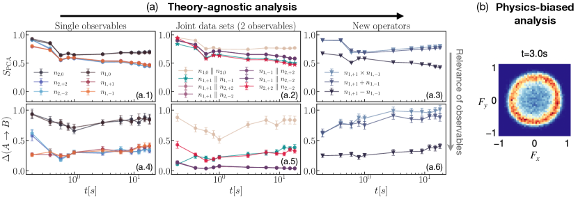
Figure 2: Assumption-free identification of relevant observables. (a) PCA entropy, $S_{\mathrm{PCA}}$, and information imbalance, $\Delta(A\to B)$, as relevance metrics of physical observables: lower values of $S_{\mathrm{PCA}}$ signal stronger correlations between the features of an observable, while lower values of $\Delta(A\to B)$ indicate that the features of a given observable (space $A$) are more informative of the full set measured features (space $B$). Both metrics clearly show that $n_{1,\pm 1}$ and $n_{2,\pm 2}$ are more relevant (in the sense above) over the full evolution [panels (a.1) and (a.4)]. Identification of relevant groups is also possible by analysing joint data sets: for pairs of observables, $n_{1,+1}\mathbin{\|}n_{1,-1}$ and $n_{2,+2}$ $\mathbin{\|}$ $n_{2,-2}$, have the lowest $S_{\mathrm{PCA}}$ [$\star$ markers in panel (a.2)] (see ranking of all possible pairs in Appendix B). Features from both ‘relevant’ pairs are in fact required to better describe space $B$ [points with $\Delta(A\to B)\sim 0$ in panel (a.5), for which $A$ is defined by the set of features of $n_{1,\pm 1}\mathbin{\|}n_{2,\pm 2}$. Note that these points are almost on top of each other.] Relevant new operators defined from the measured observables can also be identified, as illustrated here for a few combinations of $n_{1,+1}$ and $n_{1,-1}$, with $n_{1,+1}-n_{1,-1}$ being the most relevant [panels (a.3) and (a.6)]. (b) Histogram of the transverse spin variable in the $F_{x}-F_{y}$ plane at $t=3s$, featuring a ring-like structure. Based on physical arguments Prüfer et al. (2018, 2020); Stamper-Kurn and Ueda (2013); Kawaguchi and Ueda (2012), this variable is the relevant field to describe the quenched system. Our theory-agnostic approach identifies the relevant observables from which this variable is inferred [see Eq. (III)], hence cross-validating the latter analysis.

Let us now describe the structure of the collected experimental data sets analysed in this work. At each evolution time, each density is sampled linearly at $p=184$ spatial locations along the longitudinal trap direction. Such measurements are repeated so as to gather $N_{r}=225$ independent realizations. We denote a single realization of a spatial density profile by a $p$-dimensional vector $\vec{n}^{i}_{\alpha}(t)$, where the considered internal state is succinctly labelled by ${\alpha}\equiv(F,m_{F})$. Thus, for each observable (density), and at each evolution time $t$, we obtain a data set ${\bf M}_{\alpha}(t)=\{\vec{n}^{1}_{\alpha}(t),\vec{n}^{2}_{\alpha}(t),\dots,\vec{n}^{N_{r}}_{\alpha}(t)\}$, which can be represented as a $(N_{r}\times p)$ rectangular data matrix. Using the terminology of the previous section, the features of the experimental data at hand are therefore the measured densities at selected positions. Examples of single realizations at different evolution times are shown in appendix A. Further, we also consider joint data sets formed by concatenating horizontally data sets of the measured densities for different $\alpha$ at a given time. More specifically, each row in a joint data matrix is formed by appending, one after the other, single realizations of the observables of choice. Thus, for example, a joint data set of two observables will have twice as many features as the data set of one individual observable, but the same number of rows $N_{r}$. The particular order in which we concatenate the combined observables is irrelevant for our methods. When needed, we will simply specify joint data sets by using the symbol of the corresponding observables joined by “$\mathbin{\|}$”.

IV Identification of relevant observables

We now perform a descriptive analysis of the data sets above, with the goal of identifying relevant observables, that is, those observables that capture dominant spatial correlations across the evolution of the system. This is, in fact, a crucial task in order to determine good degrees of freedom emerging from the underlying physical system.

The framework presented here builds on the complementary tools discussed in Secs. II.1 and II.2. We first compute the PCA entropy of the measured spatial density profiles and their combinations, and use it as a direct probe of the spatial correlations captured by those observables at each evolution time. Next, we use information imbalance as a way to determine which observables retain more information from the full space of observations, thereby providing a complementary metric for observable relevance. Let us note that, as discussed in Sec. II.1, $S_{\mathrm{PCA}}$ cannot reveal the presence of correlations if the embedding manifold of the data is curved. On the other hand, the estimator of the information imbalance in Eq. (2) depends only on the local neighborhood of each data point, and hence is well-suited to deal with arbitrarily non-linear manifolds Glielmo et al. (2022). In this sense, ranking the relevance of observables with both techniques provides a way to cross-verify the validity of our results.

Our main results are shown in Fig. 2(a). Let us first analyze the results for the PCA entropy [panels (a.1)–(a.3)]. A clear separation between two groups of observables is noted as the system evolves [panel (a.1)], with $n_{1,\pm 1}$ and $n_{2,\pm 2}$ having lower values of $S_{\mathrm{PCA}}$. We conclude that these observables capture stronger spatial correlations and are hence more relevant in the sense specified above. Next, we consider joint data sets of two observables [panel (a.2)]. The most relevant pairs according to this analysis are $\{n_{1,+1},n_{1,-1}\}$ and $\{n_{2,+2},n_{2,-2}\}$. The latter result is in excellent agreement with the physics-motivated analysis, in which such observables play a key role in the definition of the transverse spin [see Eq. (III) and Fig. 2(b)]. Going one step further, in panel (a.3) we explore concrete functional combinations of the pair of observables $\{n_{1,+1},n_{1,-1}\}$ (similar results are found for $\{n_{2,+2},n_{2,-2}\}$), which define new operators. We find that $n_{1,+1}-n_{1,-1}$ has the lowest $S_{\mathrm{PCA}}$, once again in agreement with the physics-motivated ansatz [Eq. (III)].

We now turn our attention to the information imbalance analysis [panels (a.4)–(a.6)], which provides a complementary view on the relevance of observables. Here, $A$ refers to the space of features associated to a given observable, while $B$ is the full space of ($184\cdot 6=1104$) measured features. In panel (a.4), we can see that the observables with a lower PCA entropy have also a lower information imbalance. In other words, the observables that capture dominant spatial correlations are also more informative of the full space of data features (in the information imbalance sense). Interestingly, in the analysis of pairs of observables [panel (a.5)], we note that in order to describe the full space of observations, one needs to consider features from both of the relevant pairs. Indeed, we see that the space $A$ that combines features from the observables $n_{1,\pm 1}$ and $n_{2,\pm 2}$ have $\Delta(A\to B)\sim 0$, for the full evolution [note that the points corresponding to the four possible combinations of these observables are almost on top of each other in panel (a.5)]. The new operator $n_{1,+1}-n_{1,-1}$ has also a significantly lower information imbalance than the other considered operators in panel (a.6).

In Appendix A, we show some instances of single realizations of the measured density profiles. While one can see a certain correlation in the behavior of the identified relevant observables (at the level of single realizations), our analysis rules out, in a systematic and unbiased way, the presence of other important correlations among the measured quantities. Further results for the analysis carried out here are shown in Appendix B.

V Algorithmic complexity of the quantum dynamics

Finally, we provide a further characterization of the data sets. Specifically, we study their intrinsic dimension $I_{d}$, at the considered evolution times. This allows us to characterize the algorithmic complexity of the quantum dynamics probed in our experiment. We note that this notion of complexity is fundamentally different from computational complexity - prominent examples of the latter being entanglement Schuch et al. (2008); He and Millis (2017); Yang et al. (2017) and quantum circuit complexity Brandão et al. (2021); Haferkamp et al. (2022). In the context of quantum many-body systems, computational complexity deals in general with characterizing the number of classical resources needed to efficiently simulate a quantum state (e.g., the bond dimension of a matrix product state representation or the number of gates needed in a quantum circuit to describe a target state). On a very distinct note, algorithmic complexity quantifies the notion of compression of information in a classical object, which in our particular case refers to the classical encoding of a quantum state given by the output of measurements (or even classical calculations). We note that these two notions of complexity do not necessarily align with each other, and while the computational complexity has been explored intensively in the realm of strongly interacting systems, much less is known about the algorithmic complexity of quantum many-body states.

As explored in recent studies on critical phenomena in many-body systems Mendes-Santos et al. (2021a, b); Turkeshi (2022); Mendes-Santos et al. (2023), the algorithmic complexity does provide a physical picture of the complexity of many-body states, revealing for example an emergent simplification of the data manifold in systems featuring universality, where the physics also becomes parametrically simpler and can be described by a handful of universal exponents and functions. The present work thus extends the study of this kind of complexity to the realm of far-from-equilibrium quantum many-body dynamics.

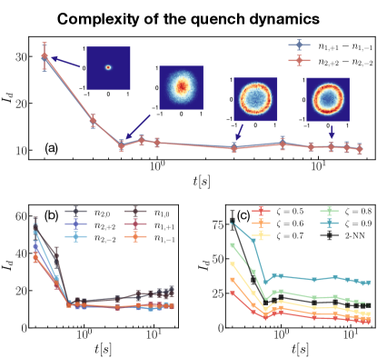
Figure 3: Intrinsic dimension as a function of time for (a) the relevant observables, $n_{1,+1}-n_{1,-1}$ and $n_{2,+2}-n_{2,-2}$, (b) all measured densities individually, and (c) joint data sets of all six observables together. In all instances, an initially large $I_{d}$ quickly decays to smaller values (around $t=0.6s$), subsequently exhibiting long plateaus. The insets in panel (a) show histograms of the transverse spin in the $F_{x}-F_{y}$ plane at selected times. The first drop in the $I_{d}$ is associated to a grow in the spin length, which remains approximately constant for $t\gtrsim 1s$. In the latter regime a ring-like structure is then observed (illustrated here at $t=3s,12s$). Spatial correlations of spin phase excitations exhibit self-similar dynamics in a regime that starts around $t\gtrsim 3s$ Prüfer et al. (2020). The observed structural simplification of the data strongly correlates with such universal dynamics. Hence, the plateaus in the plot of $I_{d}$ provide a lower bound for the onset of simpler dynamics and universal scaling. Panel (c) also shows the $I_{d}$ estimate based on PCA for various values of the cutoff $\zeta$ (see main text).

Shown in Fig. 3(a) is the plot of $I_{d}$ as a function of time, of the data sets corresponding to the identified relevant operators, $n_{1,+1}-n_{1,-1}$ and $n_{2,+2}-n_{2,-2}$. We observe the same trend in both instances: a quick decay of $I_{d}$ to considerably smaller values, subsequently displaying long, stable plateaus. The reduction of the $I_{d}$ signals a simplification of the data structure due to the buildup of correlations among the input variables. The latter is a direct manifestation of the correlations among the elementary constituents of the system. From the physical viewpoint, the post-quench correlations are associated with the formation of a ring-like structure, with approximately constant radius, in the transverse component of the collective spin degree of freedom (insets) Prüfer et al. (2018, 2020). In turn, spatial correlations of the spin phase excitations exhibit universal scaling dynamics Prüfer et al. (2018). In the present experiment, the universal scaling regime starts approximately at $t\sim 6s$ Prüfer et al. (2020). The physical basis for such scaling evolution is a dynamical reduction of the relevant parameters in the system. This is strongly consistent with the observed structural simplification of the data, as also observed in recent studies of critical behavior—in and out of equilibrium—in classical and quantum statistical mechanics systems Mendes-Santos et al. (2021a, b); Turkeshi (2022); Mendes-Santos et al. (2023). Therefore, in the present case, the observed $I_{d}$ plateau provides a theory-agnostic lower bound for the timescale after which the dynamics may become simpler, allowing for the emergence of self-similar behavior.

Importantly, this prediction can be made by directly studying the $I_{d}$ of data sets of all measured densities, as shown in Fig. 3(b), where we observe an overall similar trend. We note, however, that the “irrelevant” observables $n_{1,0}$ and $n_{2,0}$, have a growing $I_{d}$, rather than a plateau. This further confirms the relevance predictions based on PCA entropy and information imbalance. Further, in Fig. 3(c) we plot the $I_{d}$ of joint data sets of the six measured observables together, showing once again the noted trend. In this plot, we also show an $I_{d}$ estimation based on PCA, which is defined by choosing an ad hoc cutoff parameter $\zeta$, for the integrated spectrum of the covariance matrix Jolliffe (2005); Mendes-Santos et al. (2021a), i.e., $\sum_{k=1}^{I_{d}}\tilde{\lambda}_{k}\approx\zeta$. We find that for all considered values of $\zeta$, we recover the same qualitative features as the TWO-NN $I_{d}$-estimate. A quantitative agreement can also be achieved for a suitable choice of $\zeta$ in the range $0.7\leq\zeta\leq 0.9$, at the different evolution times. Since the TWO-NN estimator only depends on local neighborhoods and is therefore well-suited to deal with curved manifolds, as opposed to the PCA method, this agreement further confirms the applicability of PCA in our previous analysis and implies that curvature effects in the data manifold are negligible.

In Appendix C, we show some examples of the linear fits used to estimate $I_{d}$ as prescribed by the TWO-NN algorithm; see Eq. (3). Statistical error on the results presented in this work were computed using a version of the delete-$d$ Jackknife standard error estimator via a stochastic subsampling algorithm without repetitions Politis et al. (1999); Shao and Tu (1995), as detailed in Appendix D.

VI Conclusions

We have introduced an assumption-free method to diagnose and rank relevant correlations in the dynamics of out-of-equilibrium quantum systems. The method exploits the full spectrum of principal components, as well as recently developed techniques based on information imbalance. We have successfully identified the most relevant operators describing the dynamics of Bose Einstein condensates, confirming previous heuristic approaches (and thus, validating the physical relevance based solely on experimental observations). Utilizing manifold characterization methods, we have also found stable plateaus of the intrinsic dimension of the data sets corresponding to different times, thus providing bounds on the time frame realizing universal quantum dynamics. Our approach is immediately extended to other classes of quantum simulators—including fermion gases and lattice spin models—providing a flexible, assumption-free framework to discover physical phenomena, as well as to validate their functioning. Our work complements recent theoretical approaches with similar goals regarding the identification of relevant observables Miles et al. (2021); Bohrdt et al. (2021) and characterizing the complexity of quantum dynamics Mendes-Santos et al. (2023); Schmitt and Lenarčič (2022); Casagrande et al. (2023).

Appendix A Experimentally measured observables

In this appendix we show, for completeness, examples of single realizations of the measured density profiles at selected evolution times. We refer the reader to Ref. Prüfer et al. (2020), where the experimental data analysed in this work were taken from, for further experimental details. For the sake of clarity, we plot the density profiles corresponding to the hyperfine manifolds $F=1$ and $F=2$, separately in Figs. 4 and 5, respectively. The structure of the experimental data is as follows: before measuring the atomic densities a $\pi/2$ rotation around a transverse spin axis is performed. That means that measurements are done in the $x$- or $y$-basis. The states at the poles of the spin sphere, therefore, correspond to fully elongated spins along the $x$- or $y$-direction, respectively. At the poles one then measures all atoms in the internal states $(F,m_{F})=(1,\pm 1)$ or $(F,m_{F})=(2,\pm 2)$ Kunkel et al. (2019).

In the initial state, all atoms are in the magnetic substate $m_{F}=0$, as discussed in the main text. However, due to the applied $\pi/2$ pulse before imaging the atoms, the atomic densities get modified and the initial $m_{F}=0$ population is split between the substates $m_{F}=\pm 1$ and $m_{F}=\pm 2$, for the readouts in $F=1$ and $F=2$, respectively. This is precisely what we observe in the first row of in Figs. 4 and 5, which corresponds to $t=0.0s$. We note however that no spatial correlations are imprinted in such an initial state. This is why both the PCA entropy and the intrinsic dimension of the measured densities are initially large (see Figs. 2 and 3, in the main text). That is, the corresponding data collections at short times exhibit the largest algorithmic complexity due to the statistical independence of the input variables (densities at different spatial positions).

At later evolution times, certain correlations between atomic densities in different substates can be observed at the level of single realizations. These are a consequence of certain symmetries of the system under study. For example, rotational invariance is ultemately responsible for a conserved population imbalance between the substates $m_{F}=\pm 1$ during the spin-changing collisions that drive the spinor Bose gas out of equilibrium Stamper-Kurn and Ueda (2013); Kawaguchi and Ueda (2012). However, excluding the presence of other important correlations by direct inspection becomes very hard and one needs to rely on techniques such as the ones introduced in this work, which allow to identify dominant correlations in a fully systematic and unbiased manner.

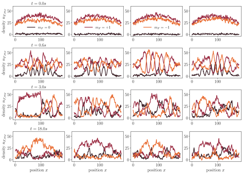
Figure 4: Experimentally observed density profiles in the hyperfine manifold $F=1$. Single realizations of the measured densities are shown at selected evolution times in the subsequent rows.

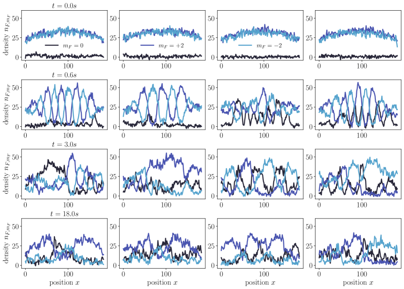
Figure 5: Experimentally observed density profiles in the hyperfine manifold $F=2$. Single realizations of the measured densities are shown at selected evolution times in the subsequent rows.

Appendix B Further results on relevant observables

In this section, we show the ranking of operators beyond the ones discussed in the main text. In particular, in panels (a.2) and (a.5) of Fig. 2, we only show results for some of the possible combinations of two of the observed densities. In Figs.  6 and 7, we show the results for all possible 15 combinations. In these plots we can better appreciate the separation into three groups of combinations. Focusing first on $S_{\mathrm{PCA}}$, we can distinguish the two most informative pairs of observables with lower values of $S_{\mathrm{PCA}}$, throughout almost the whole evolution, namely, $\{n_{1,+1},n_{1,-1}\}$ and $\{n_{2,+2},n_{2,-2}\}$ ($\star$ markers in Fig. 6). These are follow by an set of combinations—each containing at least one of the observables in the identified relevant pairs—with intermediates values of $S_{\mathrm{PCA}}$, and finally the “least” informative combination $\{n_{1,0},n_{2,0}\}$. The information imbalance in Fig. 7, reveals a similar separation. First, with an almost zero information imbalance, we have the space of features corresponding to the combinations $\{n_{1,\pm},n_{2,\pm 2}\}$ (points with a darker color in Fig. 7). This results, as discussed in the main text, means that in order to describe the full space of measured features we need to combine features from each of the two relevant pairs $\{n_{1,+1},n_{1,-1}\}$ and $\{n_{2,+2},n_{2,-2}\}$. The next group of combinations, yielding intermediate values of $\Delta(A\to B)$, contain features within only one of such relevant pairs, e.g., $\{n_{1,0},n_{1,-1}\}$ or $\{n_{2,+2},n_{2,-2}\}$. Finally, once again, we identify as the “least” informative combination that of $\{n_{1,0},n_{2,0}\}$.

Similar observations are obtained if one considers groups of more than two observables. This is illustrated here for groups of four observables (quadruplets) in Figs. 8 and 9. In terms of PCA entropy the most relevant combination is the one that combines the features of the two relevant pairs, namely, the joint data set $n_{1,+1}\mathbin{\|}n_{1,-1}\mathbin{\|}n_{2,+2}\mathbin{\|}n_{2,-2}$ ($\star$ markers in Fig. 8). We note however that in this case the relative difference in PCA entropy is not as pronounced as in the case of single or two observables. Regarding information imbalance, we observe once again those joint data sets that combine features from the two relevant pairs can predict almost entirely the full space of features. There are indeed only two combinations that only involve features from a single relevant pair (plus the two “irrelevant” observables $n_{1,0}$ and $n_{2,0}$), namely, $n_{1,0}\mathbin{\|}n_{1,+1}\mathbin{\|}n_{1,+1}\mathbin{\|}n_{2,0}$ and $n_{1,0}\mathbin{\|}n_{2,0}\mathbin{\|}n_{2,+2}\mathbin{\|}n_{2,-2}$ (square markers in Fig. 9), which clearly have a significantly larger information imbalance compared to the rest.

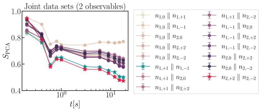
Figure 6: PCA entropy of joint data sets of two observables. This plot shows the results for all joint data sets of two observables [cf. Fig. 2(a.2) of the main text].

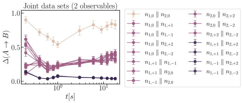
Figure 7: Information imbalance from the space of features of joint data sets combining two observables to the full space of measured features. This plot shows the results for all joint data sets of two observables [cf. Fig. 2(a.5) of the main text]. Note that the points corresponding to the joint data sets $n_{1,+1}\mathbin{\|}n_{2,+2}$, $n_{1,+1}\mathbin{\|}n_{2,-2}$, $n_{1,-1}\mathbin{\|}n_{2,+2}$, and $n_{1,-1}\mathbin{\|}n_{2,-2}$, lie basically on top of each other (they are equally informative), with an information imbalance $\Delta(A\to B)\sim 0$. These four data sets combine features of the two relevant pairs $\{n_{1,+1},n_{1,-1}\}$ and $\{n_{2,+2},n_{2,-2}\}$.

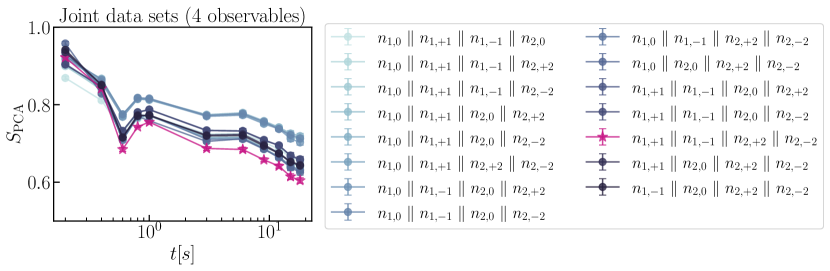
Figure 8: PCA entropy of joint data sets of four observables. The joint data set with the smallest PCA entropy is the one that combines the two relevant pairs ($\star$ markers).

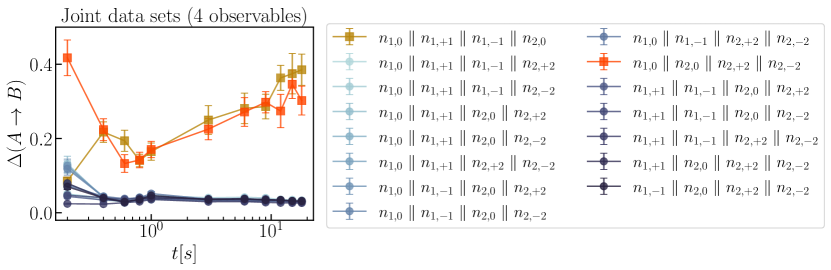
Figure 9: Information imbalance from the space of features of joint data sets combining four observables to the full space of measured features. All joint data sets that include features from the two relevant pairs $\{n_{1,+1},n_{1,-1}\}$ and $\{n_{2,+2},n_{2,-2}\}$ have a very small information imbalance. Instead, the joint data sets that only include features from one of the relevant pairs cannot predict so well the full space of features. The latter are indicated with square markers in this plot.

Appendix C Linear fit to estimate $I_{d}$ from the empirical cumulates in the TWO-NN method

In this section, we show examples of the linear fitting procedure used to estimate the value of the intrinsic dimension in the TWO-NN method; see Eq. (3) in the main text. In Fig. 10, we show the empirical cumulative distributions of the ratios $\mu_{i}=r_{i_{2}}/r_{i_{1}}$, sorted in ascending order, for the observable $n_{2,+2}-n_{2,-2}$, at all evolution times. If the condition of constant density in the range of first two nearest neighbors holds, a plot of the resulting points $\{\ln(\mu),-\ln[1-F_{\mathrm{emp}}(\mu)]\}$ will be a line that passes through the origin and whose slope gives the estimated value of $I_{d}$. Verifying that the empirical cumulates are indeed consistent with a Pareto distribution as described above, is the first step to guarantee the applicability of the TWO-NN method. Besides, on its own, this kind of plot is also very informative about the local structure of complicated data manifolds.

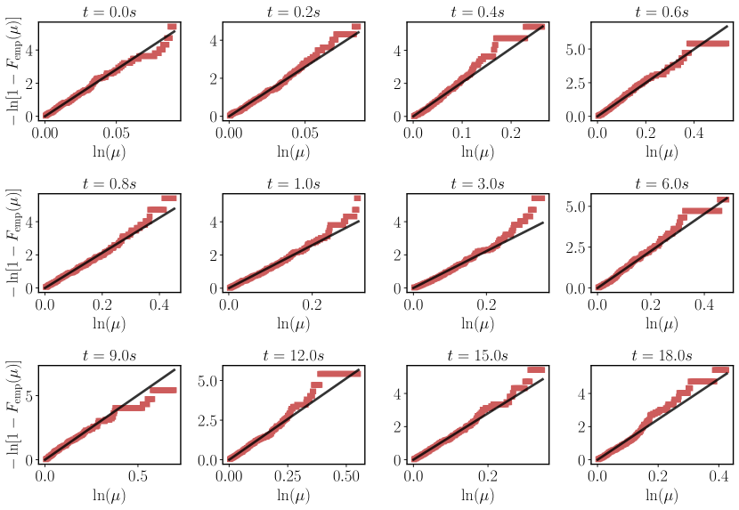
Figure 10: Empirical cumulative distributions at all evolution times for the data sets corresponding to the relevant field $n_{2,+2}-n_{2,-2}$. The black curve show the linear fit according to Eq. (3) in the main text, whose slope gives the estimated value of $I_{d}$. This procedure is valid as long as the empirical cumulative distribution function is consistent with a Pareto distribution, at least over a significant range of values of $\ln(\mu)$, as is clearly the case here.

Appendix D Subsampling error estimation

Due to the limited number of realizations used in the present analysis, we opted for using a technique known as subsampling Politis et al. (1999); Shao and Tu (1995) to have a sensible estimation of statistical errors. The subsampling algorithm is described below.

At a given time and for a given measured observable, we have $N_{r}=225$ independent realizations forming our data set, that is, ${\bf M}=\{\vec{n}^{i}\}_{i=1}^{N_{r}}$, where for simplicity we have omitted the indices labeling the internal state and the evolution time. Using these data we compute a certain numerical statistic $\vartheta$. Given two preset integers $b$ and $q<N_{r}$, the subsampling analysis proceeds as follows:

1. Form $b$ random ‘batches’ (subsamples) of data by drawing $q<N_{r}$ points at random but without replacement from the data set ${\bf M}$.

2. Estimate the statistic of interest on each subsample, that is, $\vartheta_{j}$, for $j\in\{1,\dots,b\}$.

3. Compute the mean of such estimates $\overline{\vartheta}=\frac{1}{b}\sum_{j=1}^{b}\vartheta_{j}$. The standard error can then be estimated as follows

$$\mathrm{SE}\approx\sqrt{\frac{q}{N_{r}-q}}\cdot\sqrt{\frac{1}{b}\sum_{j=1}^{b}(\vartheta_{j}-\overline{\vartheta})^{2}}.$$ (5)

This formula is known as the delete-$d$ Jackknife standard error estimator (with stochastic subsampling) Politis et al. (1999); Shao and Tu (1995).

While formally this method requires $q/N_{r}\to 0$, $q\to\infty$, and $b\to\infty$ as $N_{r}\to\infty$ (so that the distribution of the $\vartheta_{i}$ converges to the sampling distribution of $\vartheta$), in practice the choice of these parameters is problem specific. In our analysis, we did not find significant changes for $b\geq 30$. Hence, we fixed $b=30$. Furthermore, to compute a meaningful statistic on each subsample, we set $q=100$, satisfying at least $q/N_{r}<1$.

We used this method since sampling is performed without replacement. This is important as the TWO-NN algorithm used to estimate the $I_{d}$ works under the assumption of no repetitions among the data points.

References

- Bloch et al. (2008) Immanuel Bloch, Jean Dalibard, and Wilhelm Zwerger, “Many-body physics with ultracold gases,” Rev. Mod. Phys. 80, 885–964 (2008).
- Lewenstein et al. (2012) Maciej Lewenstein, Anna Sanpera, and Verònica Ahufinger, Ultracold Atoms in Optical Lattices: Simulating quantum many-body systems (Oxford University Press, 2012).
- Georgescu et al. (2014) I. M. Georgescu, S. Ashhab, and Franco Nori, “Quantum simulation,” Rev. Mod. Phys. 86, 153–185 (2014).
- Gross and Bloch (2017) Christian Gross and Immanuel Bloch, “Quantum simulations with ultracold atoms in optical lattices,” Science 357, 995–1001 (2017), https://www.science.org/doi/pdf/10.1126/science.aal3837 .
- Daley et al. (2022) Andrew J. Daley, Immanuel Bloch, Christian Kokail, Stuart Flannigan, Natalie Pearson, Matthias Troyer, and Peter Zoller, “Practical quantum advantage in quantum simulation,” Nature 607, 667–676 (2022).
- Cao et al. (2019) Yudong Cao, Jonathan Romero, Jonathan P. Olson, Matthias Degroote, Peter D. Johnson, Mária Kieferová, Ian D. Kivlichan, Tim Menke, Borja Peropadre, Nicolas P. D. Sawaya, Sukin Sim, Libor Veis, and Alán Aspuru-Guzik, “Quantum chemistry in the age of quantum computing,” Chemical Reviews, Chemical Reviews 119, 10856–10915 (2019).
- Kunkel et al. (2019) Philipp Kunkel, Maximilian Prüfer, Stefan Lannig, Rodrigo Rosa-Medina, Alexis Bonnin, Martin Gärttner, Helmut Strobel, and Markus K. Oberthaler, “Simultaneous readout of noncommuting collective spin observables beyond the standard quantum limit,” Phys. Rev. Lett. 123, 063603 (2019).
- Tsvelik (2003) Alexei M. Tsvelik, Quantum Field Theory in Condensed Matter Physics, 2nd ed. (Cambridge University Press, 2003).
- Kleinert (2018) Hagen Kleinert, Collective Classical and Quantum Fields (WORLD SCIENTIFIC, 2018) https://www.worldscientific.com/doi/pdf/10.1142/10545 .
- Alter et al. (2000) Orly Alter, Patrick O. Brown, and David Botstein, “Singular value decomposition for genome-wide expression data processing and modeling,” Proceedings of the National Academy of Sciences 97, 10101–10106 (2000).
- Varshavsky et al. (2006) Roy Varshavsky, Assaf Gottlieb, Michal Linial, and David Horn, “Novel Unsupervised Feature Filtering of Biological Data,” Bioinformatics 22, e507–e513 (2006), https://academic.oup.com/bioinformatics/article-pdf/22/14/e507/614890/btl214.pdf .
- Varshavsky et al. (2007) Roy Varshavsky, Assaf Gottlieb, David Horn, and Michal Linial, “Unsupervised feature selection under perturbations: meeting the challenges of biological data,” Bioinformatics 23, 3343–3349 (2007), https://academic.oup.com/bioinformatics/article-pdf/23/24/3343/16861997/btm528.pdf .
- Glielmo et al. (2022) Aldo Glielmo, Claudio Zeni, Bingqing Cheng, Gábor Csányi, and Alessandro Laio, “Ranking the information content of distance measures,” PNAS Nexus 1 (2022).
- Donkor et al. (0) Edward Danquah Donkor, Alessandro Laio, and Ali Hassanali, “Do machine-learning atomic descriptors and order parameters tell the same story? the case of liquid water,” Journal of Chemical Theory and Computation 0, null (0), pMID: 36920997, https://doi.org/10.1021/acs.jctc.2c01205 .
- Facco et al. (2017) Elena Facco, Maria d’Errico, Alex Rodriguez, and Alessandro Laio, “Estimating the intrinsic dimension of datasets by a minimal neighborhood information,” Scientific Reports 7, 12140 (2017).
- Facco et al. (2019) Elena Facco, Andrea Pagnani, Elena Tea Russo, and Alessandro Laio, “The intrinsic dimension of protein sequence evolution,” PLOS Computational Biology 15, 1–16 (2019).
- Allegra et al. (2020) Michele Allegra, Elena Facco, Francesco Denti, Alessandro Laio, and Antonietta Mira, “Data segmentation based on the local intrinsic dimension,” Scientific Reports 10, 16449 (2020).
- Glielmo et al. (2021) Aldo Glielmo, Brooke E. Husic, Alex Rodriguez, Cecilia Clementi, Frank Noé, and Alessandro Laio, “Unsupervised learning methods for molecular simulation data,” Chemical Reviews, Chemical Reviews 121, 9722–9758 (2021).
- Strydom et al. (2021) Tanya Strydom, Giulio V. Dalla Riva, and Timothée Poisot, “Svd entropy reveals the high complexity of ecological networks,” Frontiers in Ecology and Evolution 9 (2021), 10.3389/fevo.2021.623141.
- Caraiani (2014) Petre Caraiani, “The predictive power of singular value decomposition entropy for stock market dynamics,” Physica A: Statistical Mechanics and its Applications 393, 571–578 (2014).
- Gu et al. (2015) Rongbao Gu, Wei Xiong, and Xinjie Li, “Does the singular value decomposition entropy have predictive power for stock market? — evidence from the shenzhen stock market,” Physica A: Statistical Mechanics and its Applications 439, 103–113 (2015).
- Gu and Shao (2016) Rongbao Gu and Yanmin Shao, “How long the singular value decomposed entropy predicts the stock market? — evidence from the dow jones industrial average index,” Physica A: Statistical Mechanics and its Applications 453, 150–161 (2016).
- Chakraborti et al. (2020) Anirban Chakraborti, Hrishidev, Kiran Sharma, and Hirdesh K Pharasi, “Phase separation and scaling in correlation structures of financial markets,” Journal of Physics: Complexity 2, 015002 (2020).
- Alvarez-Ramirez and Rodriguez (2021) Jose Alvarez-Ramirez and Eduardo Rodriguez, “A singular value decomposition entropy approach for testing stock market efficiency,” Physica A: Statistical Mechanics and its Applications 583, 126337 (2021).
- Espinosa-Paredes et al. (2022) G. Espinosa-Paredes, E. Rodriguez, and J. Alvarez-Ramirez, “A singular value decomposition entropy approach to assess the impact of covid-19 on the informational efficiency of the wti crude oil market,” Chaos, Solitons & Fractals 160, 112238 (2022).
- Levina and Bickel (2004) Elizaveta Levina and Peter Bickel, “Maximum likelihood estimation of intrinsic dimension,” in Advances in Neural Information Processing Systems, Vol. 17, edited by L. Saul, Y. Weiss, and L. Bottou (MIT Press, 2004).
- Gong et al. (2019) S. Gong, V. Boddeti, and A. K. Jain, “On the intrinsic dimensionality of image representations,” in 2019 IEEE/CVF Conference on Computer Vision and Pattern Recognition (CVPR) (IEEE Computer Society, Los Alamitos, CA, USA, 2019) pp. 3982–3991.
- Pope et al. (2021) Phil Pope, Chen Zhu, Ahmed Abdelkader, Micah Goldblum, and Tom Goldstein, “The intrinsic dimension of images and its impact on learning,” in International Conference on Learning Representations (2021).
- Weng et al. (2022) Xiaojing Weng, Altai Perry, Michael Maroun, and Luat T. Vuong, “Singular value decomposition and entropy dimension of fractals,” in 2022 International Conference on Image Processing, Computer Vision and Machine Learning (ICICML) (2022) pp. 427–431.
- Prüfer et al. (2020) Maximilian Prüfer, Torsten V. Zache, Philipp Kunkel, Stefan Lannig, Alexis Bonnin, Helmut Strobel, Jürgen Berges, and Markus K. Oberthaler, “Experimental extraction of the quantum effective action for a non-equilibrium many-body system,” Nature Physics 16, 1012–1016 (2020).
- Prüfer et al. (2018) Maximilian Prüfer, Philipp Kunkel, Helmut Strobel, Stefan Lannig, Daniel Linnemann, Christian-Marcel Schmied, Jürgen Berges, Thomas Gasenzer, and Markus K. Oberthaler, “Observation of universal dynamics in a spinor bose gas far from equilibrium,” Nature 563, 217–220 (2018).
- Stamper-Kurn and Ueda (2013) Dan M. Stamper-Kurn and Masahito Ueda, “Spinor bose gases: Symmetries, magnetism, and quantum dynamics,” Rev. Mod. Phys. 85, 1191–1244 (2013).
- Kawaguchi and Ueda (2012) Yuki Kawaguchi and Masahito Ueda, “Spinor bose–einstein condensates,” Physics Reports 520, 253–381 (2012), spinor Bose–Einstein condensates.
- Berges et al. (2015) J. Berges, K. Boguslavski, S. Schlichting, and R. Venugopalan, “Universality far from equilibrium: From superfluid bose gases to heavy-ion collisions,” Phys. Rev. Lett. 114, 061601 (2015).
- Erne et al. (2018) Sebastian Erne, Robert Bücker, Thomas Gasenzer, Jürgen Berges, and Jörg Schmiedmayer, “Universal dynamics in an isolated one-dimensional bose gas far from equilibrium,” Nature 563, 225–229 (2018).
- Glidden et al. (2021) Jake A. P. Glidden, Christoph Eigen, Lena H. Dogra, Timon A. Hilker, Robert P. Smith, and Zoran Hadzibabic, “Bidirectional dynamic scaling in an isolated bose gas far from equilibrium,” Nature Physics 17, 457–461 (2021).
- Wang (2016) Lei Wang, “Discovering phase transitions with unsupervised learning,” Phys. Rev. B 94, 195105 (2016).
- Hu et al. (2017) Wenjian Hu, Rajiv R. P. Singh, and Richard T. Scalettar, “Discovering phases, phase transitions, and crossovers through unsupervised machine learning: A critical examination,” Phys. Rev. E 95, 062122 (2017).
- Costa et al. (2017) Natanael C. Costa, Wenjian Hu, Z. J. Bai, Richard T. Scalettar, and Rajiv R. P. Singh, “Principal component analysis for fermionic critical points,” Phys. Rev. B 96, 195138 (2017).
- Wetzel (2017) Sebastian J. Wetzel, “Unsupervised learning of phase transitions: From principal component analysis to variational autoencoders,” Phys. Rev. E 96, 022140 (2017).
- Wang and Zhai (2017) Ce Wang and Hui Zhai, “Machine learning of frustrated classical spin models. i. principal component analysis,” Phys. Rev. B 96, 144432 (2017).
- Ch’ng et al. (2018) Kelvin Ch’ng, Nick Vazquez, and Ehsan Khatami, “Unsupervised machine learning account of magnetic transitions in the hubbard model,” Phys. Rev. E 97, 013306 (2018).
- Khatami (2019) Ehsan Khatami, “Principal component analysis of the magnetic transition in the three-dimensional fermi-hubbard model,” Journal of Physics: Conference Series 1290, 012006 (2019).
- Turkeshi (2022) Xhek Turkeshi, “Measurement-induced criticality as a data-structure transition,” Phys. Rev. B 106, 144313 (2022).
- Jolliffe (2005) Ian Jolliffe, “Principal component analysis,” in Encyclopedia of Statistics in Behavioral Science (John Wiley & Sons, Ltd, 2005).
- Mehta et al. (2019) Pankaj Mehta, Marin Bukov, Ching-Hao Wang, Alexandre G.R. Day, Clint Richardson, Charles K. Fisher, and David J. Schwab, “A high-bias, low-variance introduction to machine learning for physicists,” Physics Reports 810, 1–124 (2019), a high-bias, low-variance introduction to Machine Learning for physicists.
- Shannon (1948) C. E. Shannon, “A mathematical theory of communication,” The Bell System Technical Journal 27, 379–423 (1948).
- Trunk (1968) G.V. Trunk, “Statistical estimation of the intrinsic dimensionality of data collections,” Information and Control 12, 508–525 (1968).
- Campadelli et al. (2015) P. Campadelli, E. Casiraghi, C. Ceruti, and A. Rozza, “Intrinsic dimension estimation: Relevant techniques and a benchmark framework,” Mathematical Problems in Engineering 2015, 759567 (2015).
- Camastra and Staiano (2016) Francesco Camastra and Antonino Staiano, “Intrinsic dimension estimation: Advances and open problems,” Information Sciences 328, 26–41 (2016).
- Li and Vitányi (2009) Ming Li and Paul Vitányi, An Introduction to Kolmogorov Complexity and Its Applications, 3rd ed. (Springer New York, 2009).
- Staiger (1993) L. Staiger, “Kolmogorov complexity and hausdorff dimension,” Information and Computation 103, 159–194 (1993).
- Vitale et al. (2023) Vittorio Vitale, Tiago Mendes-Santos, Alex Rodriguez, and Marcello Dalmonte, “Topological kolmogorov complexity and the berezinskii-kosterlitz-thouless mechanism,” (2023), arXiv:2305.05396 [cond-mat.stat-mech] .
- Mendes-Santos et al. (2023) T. Mendes-Santos, M. Schmitt, A. Angelone, A. Rodriguez, P. Scholl, H. J. Williams, D. Barredo, T. Lahaye, A. Browaeys, M. Heyl, and M. Dalmonte, “Wave function network description and Kolmogorov complexity of quantum many-body systems,” arXiv e-prints , arXiv:2301.13216 (2023), arXiv:2301.13216 [cond-mat.quant-gas] .
- Mendes-Santos et al. (2021a) T. Mendes-Santos, X. Turkeshi, M. Dalmonte, and Alex Rodriguez, “Unsupervised learning universal critical behavior via the intrinsic dimension,” Phys. Rev. X 11, 011040 (2021a).
- Mendes-Santos et al. (2021b) T. Mendes-Santos, A. Angelone, Alex Rodriguez, R. Fazio, and M. Dalmonte, “Intrinsic dimension of path integrals: Data-mining quantum criticality and emergent simplicity,” PRX Quantum 2, 030332 (2021b).
- Sadler et al. (2006) L. E. Sadler, J. M. Higbie, S. R. Leslie, M. Vengalattore, and D. M. Stamper-Kurn, “Spontaneous symmetry breaking in a quenched ferromagnetic spinor bose–einstein condensate,” Nature 443, 312–315 (2006).
- Viermann et al. (2022) Celia Viermann, Marius Sparn, Nikolas Liebster, Maurus Hans, Elinor Kath, Álvaro Parra-López, Mireia Tolosa-Simeón, Natalia Sánchez-Kuntz, Tobias Haas, Helmut Strobel, Stefan Floerchinger, and Markus K. Oberthaler, “Quantum field simulator for dynamics in curved spacetime,” Nature 611, 260–264 (2022).
- Tajik et al. (2023a) Mohammadamin Tajik, Marek Gluza, Nicolas Sebe, Philipp Schüttelkopf, Federica Cataldini, João Sabino, Frederik Møller, Si-Cong Ji, Sebastian Erne, Giacomo Guarnieri, Spyros Sotiriadis, Jens Eisert, and Jörg Schmiedmayer, “Experimental observation of curved light-cones in a quantum field simulator,” Proceedings of the National Academy of Sciences 120, e2301287120 (2023a), https://www.pnas.org/doi/pdf/10.1073/pnas.2301287120 .
- Tajik et al. (2023b) Mohammadamin Tajik, Ivan Kukuljan, Spyros Sotiriadis, Bernhard Rauer, Thomas Schweigler, Federica Cataldini, João Sabino, Frederik Møller, Philipp Schüttelkopf, Si-Cong Ji, Dries Sels, Eugene Demler, and Jörg Schmiedmayer, “Verification of the area law of mutual information in a quantum field simulator,” Nature Physics 19, 1022–1026 (2023b).
- Schuch et al. (2008) Norbert Schuch, Michael M. Wolf, Frank Verstraete, and J. Ignacio Cirac, “Entropy scaling and simulability by matrix product states,” Phys. Rev. Lett. 100, 030504 (2008).
- He and Millis (2017) Zhuoran He and Andrew J. Millis, “Entanglement entropy and computational complexity of the anderson impurity model out of equilibrium: Quench dynamics,” Phys. Rev. B 96, 085107 (2017).
- Yang et al. (2017) Zhi-Cheng Yang, Alioscia Hamma, Salvatore M. Giampaolo, Eduardo R. Mucciolo, and Claudio Chamon, “Entanglement complexity in quantum many-body dynamics, thermalization, and localization,” Phys. Rev. B 96, 020408 (2017).
- Brandão et al. (2021) Fernando G.S.L. Brandão, Wissam Chemissany, Nicholas Hunter-Jones, Richard Kueng, and John Preskill, “Models of quantum complexity growth,” PRX Quantum 2, 030316 (2021).
- Haferkamp et al. (2022) Jonas Haferkamp, Philippe Faist, Naga B. T. Kothakonda, Jens Eisert, and Nicole Yunger Halpern, “Linear growth of quantum circuit complexity,” Nature Physics 18, 528–532 (2022).
- Politis et al. (1999) Dimitris N. Politis, Joseph P. Romano, and Michael Wolf, Subsampling, 1st ed. (Springer New York, 1999).
- Shao and Tu (1995) Jun Shao and Dongsheng Tu, The Jackknife and Bootstrap, 1st ed. (Springer New York, 1995).
- Miles et al. (2021) Cole Miles, Annabelle Bohrdt, Ruihan Wu, Christie Chiu, Muqing Xu, Geoffrey Ji, Markus Greiner, Kilian Q. Weinberger, Eugene Demler, and Eun-Ah Kim, “Correlator convolutional neural networks as an interpretable architecture for image-like quantum matter data,” Nature Communications 12, 3905 (2021).
- Bohrdt et al. (2021) A. Bohrdt, S. Kim, A. Lukin, M. Rispoli, R. Schittko, M. Knap, M. Greiner, and J. Léonard, “Analyzing nonequilibrium quantum states through snapshots with artificial neural networks,” Phys. Rev. Lett. 127, 150504 (2021).
- Schmitt and Lenarčič (2022) Markus Schmitt and Zala Lenarčič, “From observations to complexity of quantum states via unsupervised learning,” Phys. Rev. B 106, L041110 (2022).
- Casagrande et al. (2023) Heitor P. Casagrande, Bo Xing, Marcello Dalmonte, Alex Rodriguez, Vinitha Balachandran, and Dario Poletti, “Complexity of spin configuration dynamics due to unitary evolution and periodic projective measurements,” Phys. Rev. E 108, 044128 (2023).